
Submitted:
25 March 2025
Posted:
26 March 2025
You are already at the latest version
Abstract
This study investigates the Holocene evolution of the Laraquete-Carampangue strandplain (LCS) on the tectonically active coast of south-central Chile using Ground Penetrating Radar (GPR) and LiDAR data. Laraquete-Carampangue strandplain (LCS), on the tectonically active coast of south-central Chile, is a rare accretionary feature in a region dominated by rocky shorelines and limited sediment supply. LiDAR-derived digital elevation model reveals a complex geomorphology comprising 52 beach ridges, aeolian dunes, and fluvial paleochannels, while GPR radargrams uncover marine and aeolian facies influenced by past seismic and climatic events. We interpret these units in the frame of past seismic and climatic events. Our geomorphological and stratigraphic findings suggest that the strandplain progradation was driven by relative sea-level changes associated with past seismic cycles and Holocene climate change. We propose that the transition from drier to humid conditions in the late Holocene triggered the onset of dune formation at the end of the Little Ice Age. This integrated approach highlights the interplay of tectonic and climatic forcings in shaping coastal landforms, offering insights into their long-term response to environmental change.
Keywords:
strandplain
; Holocene
; LiDAR
; GPR
; tectonic
; climate change
; Chile
1. Introduction
A strandplain (or beach ridge plain) is a surface of sediment accumulation formed by sequences of beach ridges parallel or semi-parallel to the current coastline [1,2]. Beach ridges represent paleo-beach berms, ancient coastal barriers, or submarine bars and may be accompanied and covered by sand sheets, dunes, or paleo dunes. Therefore, some authors may also have mixed origins: marine-eolian [1,2,3]. Depressions or swales can be distinguished between ridges, corresponding to ancient runnels, interbar grooves (e.g., swash bars), or interdune depressions. The strandplains typically form in sandy coasts with high long-term sediment availability, representing a plain with net progradation (e.g., [4,5,6,7]) and can develop during a marine transgression or regression but also during a period of sea level stability [1,2,8,9]. However, they have also developed on tectonically active coasts, where relative sea level change occurs (e.g., [10,11,12]).
Strandplains have been used to study the Holocene evolution of coastal landscapes [9,13], providing keys to understanding the drivers of geomorphological changes, such as climate changes (e.g.,[6,14,15,16,17,18] ) and the related seismic cycle (e.g., [11,19,20,21,22]). Multiple tools, techniques, and methods have been used and combined to study the strand plain and its geomorphic and sedimentological components (e.g., aerial photographs, satellite images, use of trenches, sediment cores, OSL dating, among others), highlighting the use of Ground Penetrating Radar (GPR) (e.g., [3,7,14,17,20,23,24,25,26,27] and LiDAR data (e.g., [6,28,29,30,31].
GPR is a non-invasive tool that examines a landform's internal stratification and facies, offering key insights into its formation and evolution [32]. The GPR emits electromagnetic waves in the megahertz frequency range (typically 50-1000 MHz) that penetrate the subsurface and are reflected when, in its propagation, it encounters a separation surface concerning another medium. In the radargrams (a graphical representation of the data obtained), the resistivity changes of the materials are distinguished, such as a change between sand and a paleosol or a layer with a concentration of dielectric minerals (e.g., heavy minerals), recording characteristics such as morphology, inclination, and depth [32].
LiDAR, a remote sensing tool, employs laser pulses to measure the elevation of the surface and overlying features like vegetation [33]. Two main types exist: Terrestrial laser scanning (TLS), conducted from the ground, and airborne laser scanning (ALS), which is deployed from an aircraft. ALS (used here) determines topographic elevation by measuring the round-trip travel time of laser pulses from the aircraft to the surface and back [34]. LiDAR data-derived products (e.g., DTM) have been widely used in coastal geomorphology studies because they allow 2D and 3D analysis at high resolution (centimeter accuracy), which makes them ideal for the description, analysis, and counting of ridges on strandplains (e.g., [6,30]).
Chile faces a subduction zone, where the Nazca Plate subducts beneath the South American Plate (Figure 1a) at a rate of approximately 6.6 cm/year [35]. This tectonic setting has shaped the local geomorphological dynamics and long-term sediment availability for various coastal systems. Coasts along active margins are typically narrow, situated close to subduction trenches, exhibit irregular relief, reach high elevations, and display significant crustal faulting [36]. As a result, these regions feature small basins with low sediment production. Additionally, submarine canyons are common along active margins and exhibit steep slopes, often extending to the surf zone. Consequently, a significant portion of the sediment reaching the coast is transported toward these canyons, reducing the sediment available for alongshore currents that supply sandy coastal systems. Therefore, the sedimentary environments of coastal systems along active margins are discontinuous and limited in extent, resulting in predominantly rocky coasts [36].
The Chilean coast is representative of an active margin with only ~580 km of sandy coastline, representing 2% of the country's total, while the remaining 98% corresponds to rocky coasts [37]. In this setting, the presence of accretionary plains such as strandplains is limited due to the existing restrictions for their development, with the scarcity of space and the availability of sediment the main limiting factors. This is why they constitute a geomorphological singularity that should be studied not only for its uniqueness but also for its value as a system that, being less dynamic than other types of sandy coasts (e.g., beaches with dune fields), allows the recording and preservation of evidence of past events that determined the evolution of the coast.
In the following, we offer findings about the evolution of the remarkable Laraquete-Carampangue strandplain (LCS) in the Gulf of Arauco, south-central Chile. The singularity of this strandplain lies in its sediment source, which corresponds to a coastal basin of the Carampangue River, usually smaller than the Andean basins and, therefore, has a more limited sediment stock. Using LiDAR data and radargrams obtained from GPR profiles, we analyze the geomorphology and stratigraphy of the strandplain to understand the environments and processes involved in forming Holocene landforms. Our results suggest that permanent tectonic uplift and past climate changes are main drivers of its evolution and morphological changes. The findings presented here represent an excellent opportunity to comprehend the evolution of this type of sandy coast and provide the scientific basis for understanding their response to phenomena derived from climate change and the seismic cycle.
2. Study Area
The LCS is a no-deltaic strandplain [38]. Bounded to the NNE by the Laraquete River, to the E by marine terraces, to the S by the Lia River, to the SSW by the Carampangue River, and to the W by the Pacific Ocean (orange box in Figure 1c and Figure 2). The LCS lies along the coast overlooking the Gulf of Arauco in the Biobío Region, south-central Chile (red box in Figure 1c). This coastal area forms a geomorphological system approximately 100 km long, featuring another strandplain to the north, the San Pedro-Escuadrón (SSPE in Figure 1c). The coastal system developed through tectonic and eustatic processes, primarily shaping relative sea-level changes that governed its evolution during the Pleistocene and Holocene [39,40]. The geomorphological boundary between the Pleistocene and Holocene is marked by inactive cliffs separating uplifted marine terraces (Pleistocene) from the strandplain (Holocene). Three uplifted terrace levels have been mapped in the area, with the lowermost formed in the Marine Isotope Stage (MIS) 5e, about 125 ka ago, which is found at elevations ranging from 25 and 50 m [41]. The inactive cliff exhibits evidence of marine erosion related to the mid-Holocene highstand [42] or last maximum marine transgression dating to ~7-6 ka BP [39,40]. After the mid-Holocene highstand, continuous relative sea-level decrease created accommodation space for the development of the LCS.
The current climate of the study area is controlled by the Southeast Pacific Anticyclone (SPA) and the migratory pressure systems of the circumpolar flow and band associated with frontal systems [43]. The average annual precipitation is 1100 mm, and most of this precipitation is concentrated in winter, with 5 to 15 several days precipitation events [44]. Holocene evidence in south-central Chile has shown a multi-millennial climatic variability of transition from drier (middle Holocene) to more humid conditions (late Holocene) [45,46,47,48,49,50]. In front of the Gulf of Arauco, Francois et al. [51] suggest, based on the interpretation of sedimentological records from Laguna Verde (36º47’S, see Figure 1c), that a local humid period was established from ~4 ka BP, resulting from a transition from a drier period established in the middle Holocene. Lamy et al. [52] suggest that this transition was primarily driven by the transfer of the southward and northward shifts of the Southern Westerly Wind Belt (SWW), respectively, which may have influenced the increase and decrease of SPA influence.
The coastal system is located in the southern section of the 2010 Maule earthquake (Mw 8.8) (Figure 1b). This event had a ~500 km rupture and a complex slip distribution with two maximum slip patches of ~17 m and ~12 m in the northern and southern sectors of the rupture, respectively [53,54]. The earthquake caused tsunami waves and land uplift on the mainland and Santa María Island in front of LCS [55]. In Tubul, ~1.4 m of uplift was recorded, causing a widening of the beaches bordering ~100 m [56,57], while Santa María Island rose ~2.2 m, causing similar beach growth [22]. The predecessor to the 2010 Maule event was the 1835 earthquake, and comparable evidence, such as coastal uplift and tsunami inundation, suggests that both were similar [55,58,59]. Charles Darwin studied its effects in situ and quantified coastal uplift based on dead mussels still attached to the emerged rocky shore, measuring an uplift of ~2.1 m at Tubul and ~3 m at Santa María Island [60]. This coseismic uplift also triggers beach growth.
After the 2010 earthquake, vertical deformation was measured in the San Pedro-Escuadrón strandplain, the city of Coronel [61], and Santa María Island [12]. The subsidence is probably triggered because the coast facing the Gulf is in an interseismic phase, as it occurred after the 1835 earthquake [12,62]. This context, plus others associated with climate change, could partly explain the erosion phenomena of the coastline recorded on the coasts of the Gulf, including that facing the LCS [63].
The LCS is a populated coast, and the two main towns on its surface are Laraquete and Carampangue. The area has significant economic activities and infrastructures, such as a cellulose factory and a road (see Figure 2). All these populated areas and activities have expanded at the expense of the strandplain and the dune field covering part of it. The above has implied a difficulty when studying its geomorphology and stratigraphy.
3. Materials and Methods
3.1.1. LiDAR Data and other Remote Sensing Data
For accurate identification of coastal landforms, ground observations made in 2023, satellite images, an aerial photograph, and airborne Light Detection and Ranging (LiDAR) data obtained in 2008 were used. The LiDAR-derived point cloud data had a density of 2-4 points/m2 and was filtered to produce a Digital Terrain Model (DTM) with 1 m resolution. The DTM was manipulated in ArcMap 10.8 and Global Mapper Pro software. Swath profiles based on LiDAR information were created using the Extract swath profiles tool of the ArcMap 10.8 software. The satellite images used in this work come from Google Earth Pro software for 2002, 2009, and 2023. The aerial photograph used in Figure 4 was obtained from a Chilean Aerophotogrammetic Service (SAF) flight in 1979, at a scale of 1:30,000. The beach ridges counted and shown in Figure A1 were performed using the DTM in combination with aerial photographs and satellite images.
3.1.2 GPR and Terrain Data Collection
GPR data were obtained in 2023 using GSSI UtilityScan with a 350 MHz antenna with a sampling interval of 0.02-0.03 m. An Emlid Reach RS2+ differential GPS was used for topographic correction of the GPR profiles, where one of the antennas was mounted on the GPR structure. The radargrams obtained were post-processed using Radan 7 software and the Matlab MatGPR R3 package [64]. We followed a standard processing routine to process the data with default settings, which included dew (desaturation), zero-time correction, horizontal background removal, gain functions, bandpass filtering, and topography correction. The results of the transects should be accompanied by the excavation of a pit for a proper interpretation of the results (see Figure B1), as suggested by authors such as de Pinegina et al. [27] and Switzer et al. [32]. For the proper interpretation of the radargrams, different works carried out in the context of strandplain studies were used as references (e.g., [31,65,66,67,68,69,70,71,72]).
The location of the transects carried out to obtain the GPR profiles is justified in order to represent the modern and oldest landforms of the strandplain. The GPR1 profile was 400 m long, located north of the LCS, covering the current beach, the pre-2010 earthquake beach, and the vegetated dunes. The GPR2 profile was 75 m long and carried out in the coast's center between the Carampangue and Laraquete rivers, covering the modern beach and the pre-2010 earthquake beach. The GPR3 line was 250 m long and was carried out inland, in the center of the LCS, covering three beach ridges (R1, R2, and R3) and three swales (S1, S2, and S3).
4. Results
4.1. LCS Geomorphology Revealed by LiDAR Data
LCS Exhibits marine landforms, which are presented like a sequence of multiple beach ridges (Figure 2); aeolian landforms represented by a vegetated dune field near the shoreline that decreases in width as it moves away from the Carampangue River (Figure 2); and fluvial landforms: a floodplain composed of a series of paleochannels and oxbows (yellow arrows in Figure 2) located between the strandplain and the marine terraces. 52 SE-NW beach ridges were counted, similar to the current shoreline (Figure A1). DTM also reveals that the dune field apparently covers some ridges, as indicated by the orange arrows in Figure 2, at the boundary between the dune field and the beach ridges. Also, past fluvial activity, evidenced by the existence of the floodplain, has eroded the beach ridges. Patches of strandplain have become isolated due to fluvial erosion (red arrows in Figure 2; Figure 3). The water source for these channels, which are currently mostly dry, comes from coastal basins, such as those found on marine terraces and the Cost Range.
Swath profiles indicate that the strandplain does not exceed an average elevation of ~10 m, and the lowest zone is close to one-meter elevation, specifically in the paleochannel zone (A-A’ profile in Figure 3). The forest plantations on the vegetated dune reach more than 15 m elevation, higher than the dune and the strandplain itself. Also, the swath profiles show that the dunes interlock with the beach ridges, covering them and increasing the altitude of the LCS (Figure 3).
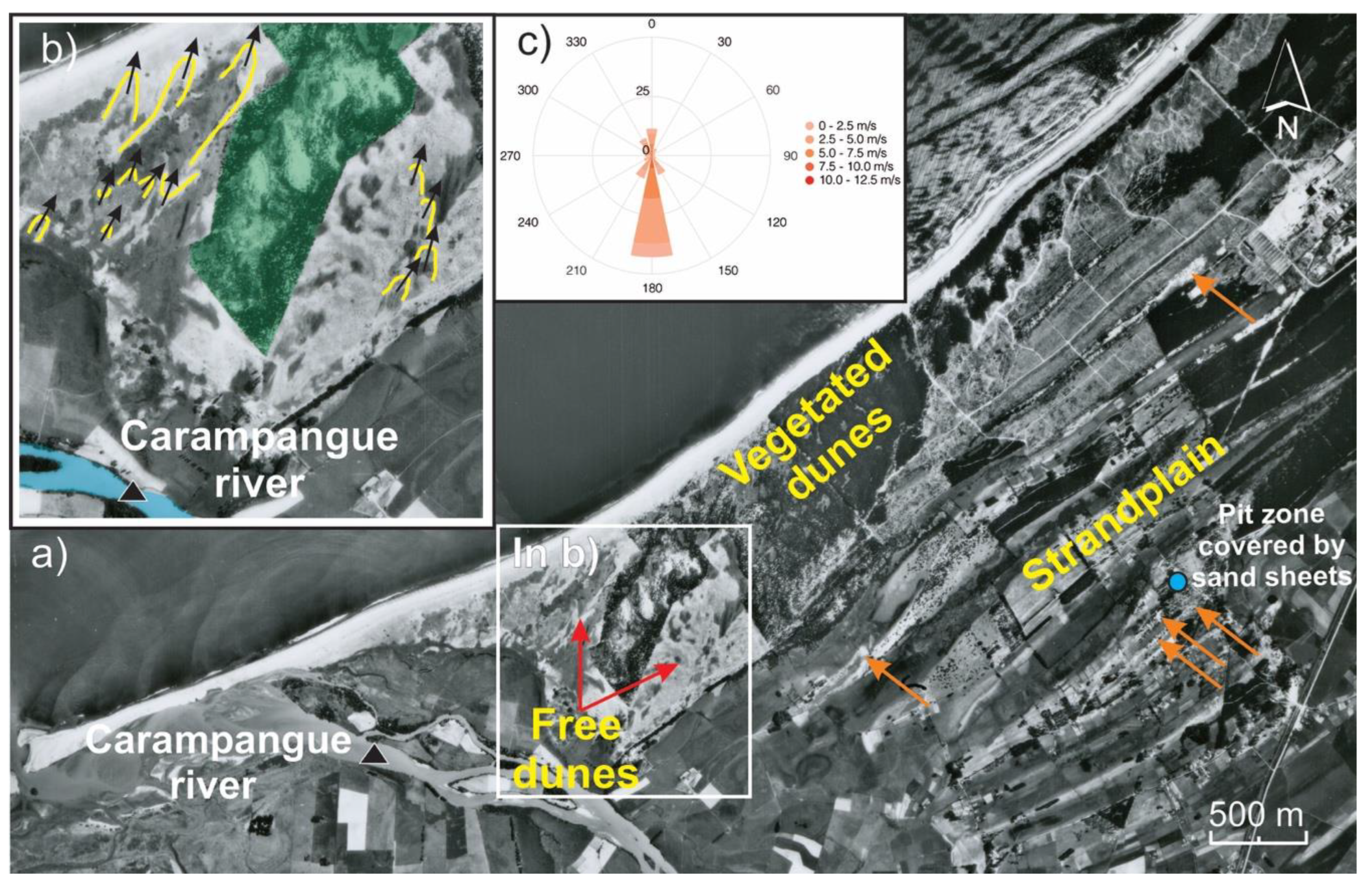
The 1979 aerial photograph (Figure 4a) confirms the free dunes and sand sheets covering the strandplain. The dunes morphology and the lack of vegetation cover indicate that they were active and advancing at the time. The direction of their movement derived from their transverse axis suggests that their sediment source was directly the river and not the sea (black arrows in Figure 4b). The direction of their movement derived from their transverse axis suggests that their sediment source was directly the river and not the sea (black arrows in Figure 4b). This is corroborated by observing the wind rose obtained for the area (Figure 4c), which shows effective wind speeds for transporting sand-sized sediment (>4.5 m/s) and coming mainly from the S, i.e., precisely from the river. The width of the dune field decreases towards the NE, from ~1200 to ~100 m, over a ~10 km extension towards Laraquete (see Figure 2), suggesting that its main sediment source is the Carampangue River. Sand sheets free of vegetation covered beach ridges and swales, including our pit (see Figure B1), implying that part of the river sediment was advancing inland in a dispersed deflation process (orange arrows in Figure 4a).
Figure 4.
Dunes in LCS. (a) Orange arrows indicate aeolian landforms (sand sheets and dunes) covering beach ridges, and the light blue circle shows the location of the pit of Figure B1, which in 1979 had a sand sheet on the surface. (b) Yellow lines indicate free dune ridges, parabolic and barchan, with an advance axis in an NE direction represented by black arrows. In green, a forest management area is indicated to control dune advance. (c) Wind rose representative of the area (reconstruction of data from 1980 to 2017, https://eolico.minenergia.cl/exploracion) shows the preferred direction of the effective winds for dunes (over 4.5 m/s) from the S. Source: Author's elaboration based on Aerophotogrammetic Service (SAF) 1979 aerial photography.
4.2. LCS stratigraphy Revealed by Radargrams Obtained from GPR Profiles
The Mw 8.8 earthquake on February 27, 2010, generated coseismic uplifts in the study area and triggered beach growth, forming new shorefaces, beachfaces, berms, and backshore. Thus, the earthquake provided an excellent opportunity to review modern analogs of recent beach facies with GPR because it allowed the pre-earthquake beach to be removed from the marine environment and away from salt water (electromagnetic waves are disturbed by salt water). Changes in the shoreface and the runnel located on the backshore can be seen in satellite images from 2002 and 2023, the year in which the GPR profiles were taken (Figure 5b). The pre-earthquake parts of the beach were identified (marked with an asterisk in Figure 5a), serving as an analog for analyzing the facies found further inland.
Sand sheet with a thickness < 1 m is seen from the back beach to the pathway (between ~80 and ~180 m), which then increases in thickness to more than 1 m towards the inland, up to almost ~400 m (Figure 5a). Underlying deposits of marine origin with shoreface facies zones (SFZ) and beachface and berm facies zones (BBZ) are present in pairs up to the road (Figure 6a and Figure 7a). After the road, the SFZ disappeared, possibly because they could not be recorded due to the dissipation of the GPR waves and/or the presence of salt water. Also, dune facies zones (DFZ) begin to be seen from the path, which become more regular in the last ~70 m of the profile.
The GPR2 profile in Figure 6a shows a configuration similar to the first ~120 m of the radargram in Figure 5a. The SFZ and BBZ are shown in sequences of alternating pairs, and at a certain point, at ~40 m, where the rear beach ends, they are covered by a sand sheet. Unlike the GPR1 profile area, where the beach was wider (~80 m), the beach identified in the GPR2 profile was narrower (~40 m). The SFZ and BBZ facies prior to the earthquake (with an asterisk in Figure 6a), were found to be more compressed or close together (up to ~60 m) than the GPR1 radargram (up to ~115 m, with an asterisk in Figure 5a). Satellite images confirm the formation of a new post-earthquake shoreface, identified as SFZ at ~15 m (Figure 6b). Also, the radargram shows that the sand sheets do not exceed ~1 m in thickness.
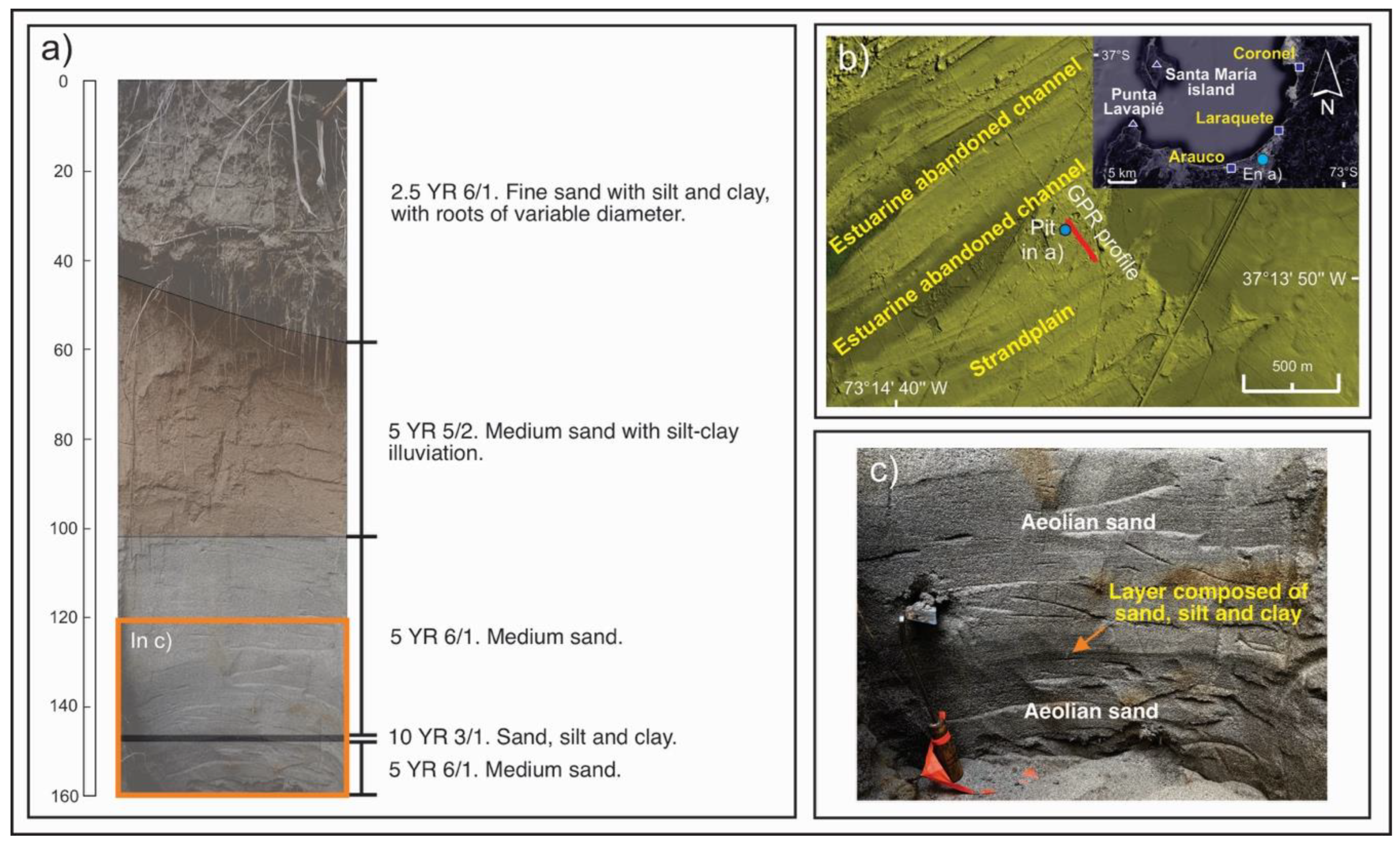
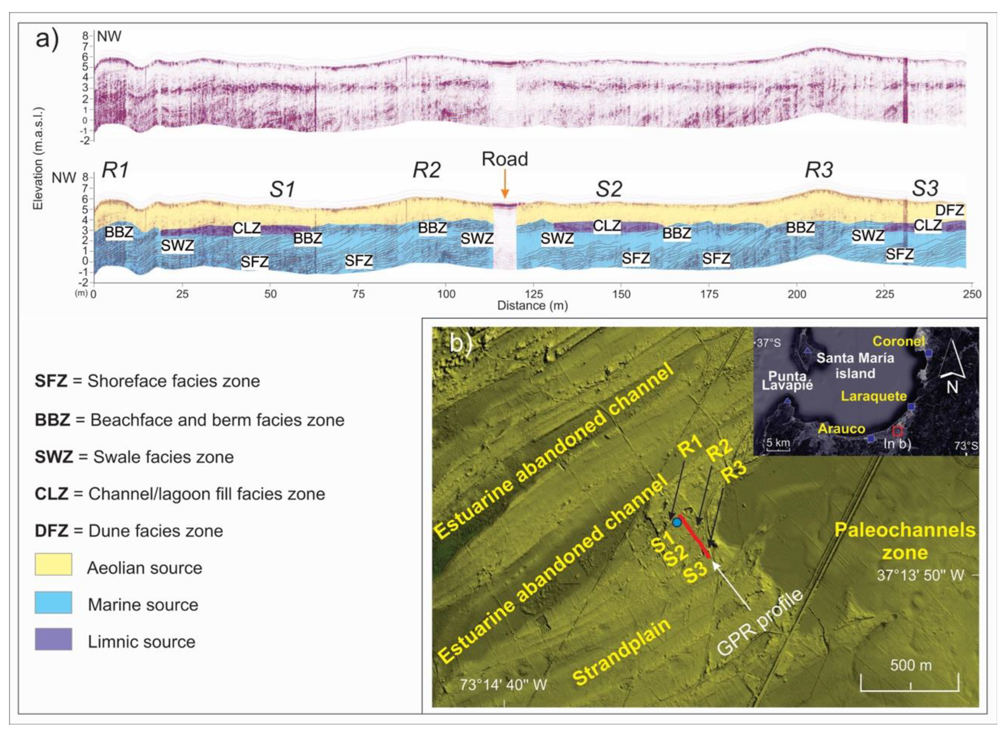
The GPR3 profile in Figure 7a was acquired approximately ~2.3 km inland within the strandplain to investigate paleofacies, using modern analogs derived from the radargrams presented in Figure 5a and Figure 6a. The profile reveals low-relief aeolian structures characteristic of sand sheets, with localized occurrences of dune facies (DFZ) exhibiting a maximum thickness of approximately ~2 m (Figure B1). Within the uppermost ~60 cm, a poorly developed soil is observed, characterized by silty clay textures, oxidized sands, and the presence of roots. This transitions to predominantly medium-grained sand below a depth of 1 m. Additionally, a silt layer, approximately ~5 cm thick, is identified at a depth of about ~150 cm (Figure B1). This layer likely represents a deposit formed by stagnant water or a limnic process, a phenomenon commonly observed in low-lying coastal topographic features, such as interdune depressions (e.g., interdune ponds).
Below the strata of aeolian origin, marine deposits corresponding to SFZ, BBZ, and swale facies zones or SWZ are observed. The SFZ and BBZ structures occur in paired sequences, resembling modern analogs of recent beaches (see Figure 5a and Figure 6a), indicating that each shoreface is associated with a corresponding beachface and berm zone. In swale-dominated zones (beneath S1 and S2), the SFZ and BBZ are spatially compressed, whereas in ridge-dominated zones (beneath R2 and R3), they are more widely separated and extensively developed. Additionally, beneath the ridges (R1, R2, and R3), the BBZ structures attain a greater vertical extent.
Furthermore, the radargram reveals an area characterized by sub-horizontal to slightly concave, semi-continuous, and compact reflectors associated with swales S1, S2, and S3. These reflectors are identified as channel-and-lagoon fill zones (CLZ) of lacustrine origin. This interpretation is particularly significant within the sedimentological and geomorphological context of inter-ridge depressions, where these zones are situated above marine deposits and below aeolian deposits. These depressions are also adjacent to abandoned estuarine channels, which may have flooded the area during their active phase, indicating a depositional environment characterized by increased humidity. Consequently, the CLZ likely represents lagoons or stagnant water bodies where both sand and finer sediments, such as silt, were deposited. This is consistent with observations from the pit shown in Figure 2a, although the CLZ exhibits greater thickness.
5. Discussion
The geomorphological analysis, based on LiDAR data and the interpretation of the GPR profiles, reveals that the strandplain has been formed mainly by a combination of marine and aeolian sedimentation processes, where dunes and sand sheets have covered landforms such as beach ridges. Our data suggest that beach ridges can be associated with landforms of aeolian origin, configuring themselves as marine-aeolian plains, as in several coasts worldwide [1,2,3]. Past fluvial processes in a greater humidity climatic phase have reconfigured the strandplain by erosive process, thereby reducing its area.
The hydrologic network, originating from the marine terraces and the Coast Range, has played a significant role in the evolution of the strandplain for two primary reasons: first, it has delivered sediments to the system [73]; and second, it has eroded the strandplain, as indicated by the development of floodplains with paleochannels that have eroded the beach ridges. These eroded beach ridges suggest that the strandplain was once more extensive and characterized by a predominantly marine sedimentation environment, which was later dominated by fluvial activity in certain sectors of the plain. In South-Central Chile, climatic variations have further influenced this evolution, with drier conditions during the Middle Holocene and wetter conditions during the Late Holocene compared to the present [45,46,47,48,49,50,51,74]. The scarcity of rainfall and surface runoff during the drier phases likely favored the formation and preservation of coastal landforms such as beach ridges. Conversely, the wetter phases promoted the development of a denser and more active hydrological network than the present-day network.
Phases of higher humidity can also be inferred from the facies visible in the radargrams, specifically in the GPR3 profile, which was obtained at ~2.3 km from the coast. In this profile, reflector packages (CLZ) are displayed that are different from those assigned to aeolian and marine origin facies are observed, whose location coincides with geomorphologically depressed zones or swales. The reflectors have a medium to low amplitude, are compact, semicontinuous, subhorizontal, and are eventually slightly concave. These layers represent changes or alterations in the sedimentation regimes in the strandplain and can be directly associated with changes in the climate [67,75]. CLZ deposits may indicate a limnic origin, like areas of recurrent flooding, swamps with coastal vegetation development, and accumulation of organic remains associated with layers with soils containing silt and clay (e.g., peat) [65,67,72,75]. It is important to note that the GPR3 profile is close to an estuarine abandoned channel (formed in wetter conditions, see Figure 7), which could have supplied water and humidity in wetter phases to the swale, keeping the water table high or near to the surface.
Furthermore, the CLZ, despite being separated by distances of tens of meters (see Figure 7), are found at a similar altitude (between 2 and 3 m), which may serve as indicators of past coastal water table levels. In addition, subhorizontal and semicontinuous reflectors are observed in the backshores and runnels of the GPR1 and GPR2 profiles, corresponding to depressed areas downwind of the berms. These facies, typical of such areas, form part of washover deposits [69,71,72]. When these depressed areas are no longer influenced by marine processes (e.g., triggered by tectonic uplift), they may develop into swale zones. Over time, the areas may become flooded, forming lagoons and swamps, with subsequent development of vegetation and even soils, generating facies similar to those observed in the CLZ (e.g., [67,75]).
The dune field located north of the Carampangue River decreases in width as it extends away from the river, indicating that the river is its primary sediment source. Our data shows that the dune fields are not present in the interior of the strandplain but instead form a sand sheet that covers the crests of the beach in some areas (Figure 4). These observations suggest that their presence results from an environmental change that promoted their formation and expansion. The primary for the formation and growth of dune fields is the availability of dry sand alongside sufficient space and effective wind (e.g., [76]). This indicates that the Carampangue River, the primary sediment source in the study area [73], either did not deliver sufficient sediment or local environmental conditions were not conducive to generating accumulation until a shift in these conditions occurred. According to our results, while the effective wind is present today (see Figure 4), the supply of dry sand from the river remains limited.
Albert studied this dune field in 1900 [77], classifying it as one of the most active in central-southern Chile during the 19th century. This significantly affected local productive activity and critical infrastructure, so the locals had to control it with pine trees (e.g., Pinus insignis). Notably, Albert dates the origin of dune fields in the region to 70 and 90 years before his work (1900). Thus, before the first half of the 19th century, there was no record of dune formation and activity in this area of Arauco that would affect the local population.
The last significant phase of global climate change prior to the 20th century was the Little Ice Age (LIA), which occurred between the 14th and 19th centuries [74]. In south-central Chile, the LIA was characterized by increased rainfall and flooding, persisting until at least the first half of the 19th century (e.g., [46,47,78,79]). However, some studies suggest that the LIA also featured dry conditions interspersed with wetter periods [74], a variability that likely influenced sediment dynamics. Consequently, the alternation between high-humidity phases and drought may have created conditions conducive to dune field formation. This could be explained by the fact that, despite high-humidity conditions over the last 2 ka BP ascending in South-Central Chile, which likely produced abundant sand-sized sediment, this sediment could only contribute to dune field formation if it remained dry for a sufficiently prolonged period to be transported and accumulated [76]. Such conditions were likely facilitated by periods of drought when sediment remained available in the system. These optimal conditions may have been particularly pronounced during the waning phase of the LIA in the first half of the 19th century, as humidity gradually decreased, allowing sediment to remain dry for extended periods. In addition to climatic factors, tectonic events may have further contributed to dune formation, as the 1835 earthquake, similar to the 2010 earthquake, caused seismic uplift [62] that likely expanded the size of the beaches. Consequently, the increased surface area facilitated the deposition and accumulation of sand, which was subsequently transported inland by wind to form the dunes.
A similar geomorphological situation has been registered in Santa María Island, located 25 km seaward, where high dune ridges (~3 m) are present near the coastline within a strandplain dominated by beach ridges, with the absence of dune fields inland. Aedo et al. [12] recorded the exceptional presence of these dunes and dated their maximum formation age of 170 years ± 15 BP (see Fig. S10 in [12]) without identifying their specific origin. A comparable situation is observed in the Moruya strandplain in Australia, where highlighting the presence of anomalous dune crests close to the coastline, which contrasts with 7 ka years of the formation of beach ridges dominant on the surface, which were formed in the mid-nineteenth century [31,66]. This mid-nineteenth century timing aligns with the waning phase of the Little Ice Age and the 1835 earthquake discussed earlier, suggesting that a combination of climatic and tectonic factors facilitated dune formation across the region during this period. These antecedents, combined with the observations of Albert [77] and the evidence collected in this study, provide a temporal context for relatively dating the formation of the dune field in the study area. However, further research is needed, including collecting data on analogs in other parts of Chile and the southern hemisphere and obtaining absolute dating data.
Finally, although the marine facies, based on their structure (e.g., inclination) and relative location, indicate the presence of ancient beaches undergoing constant accretion or progradation during at least the Middle and Late Holocene, the local sediment supply conditions are not conducive to forming a strandplain with the characteristics of the LCS. This can be attributed to the fact that its primary sediment source, the coastal basin of the Carampangue River, is a small basin with a low sediment supply potential compared to the Andean basins of Chile (e.g., Biobío River), and particularly compared to basins associated with other strandplains of similar characteristics [38]. The evidence presented in this study suggests that the Holocene accretion condition of this plain is fundamentally due to the tectonic conditions of coseismic uplift and beach growth during large earthquakes. The keys to this tectonic accretion of the beach were provided by the February 2010 earthquake, which, as seen in Figure 5 and Figure 6, caused coseismic beach growth of tens of meters. Added to this is the event of its predecessor in 1835, which also triggered an uplift [62] that must have also resulted in beach accretion, and the net uplift recorded for the study area during the Holocene, which reinforces the idea that the presence of the LCS is primarily due to the seismic cycle. It is therefore necessary to verify this tectonic influence in other coastal plains in Chile with limited sediment supply from coastal basins. While tectonic processes dominate, this study has demonstrated that climatic forcing also plays a significant role in the evolution of such tectonically active sandy coasts
6. Conclusions
The evidence provided here, obtained through LiDAR and GPR data, suggests that the evolution of the Laraquete-Carampangue Strandplain (LCS) during the middle and late Holocene was marked by three distinct phases, each dominated by environments that shaped its landforms. The first phase, initiated after the transgressive maximum of the middle Holocene in a drier climate than the present one, was characterized by the formation of marine landforms, as evidenced by multiple beach ridges constituting this plain. The second phase, predominant during the late Holocene until the Little Ice Age (LIA), was influenced by increased environmental humidity that densified the drainage network, leaving as testimony flood plains and paleochannels that eroded the strandplain. The third phase, more recent and briefer, began in the 19th century during and after the weakening of the LIA, when the alternation of wet and dry conditions favored the development of an extensive dune field north of the Carampangue River.
Regarding the presence of the LCS on the coast of the Gulf of Arauco, the sedimentary contribution of the Carampangue River, a small coastal basin, has not provided sufficient sediments to support the formation of the strandplain. Although the humid phases of the late Holocene may have been the most favorable to produce sediments, the evidence indicates that these conditions also intensified the fluvial erosion of the strandplain. On the contrary, during the middle Holocene, characterized by a drier climate and lower sedimentary contribution, the formation of beach ridge sequences that gave rise to the LCS was recorded. Meanwhile, throughout the Holocene and during the three phases of formation identified, a net decrease in relative sea level driven by tectonic uplift of the system [42]. This last point is especially relevant because, in the face of a limited sediment supply after the transgressive maximum, permanent coastal uplift was the main forcing factor responsible for the formation and permanence of the LCS.
We believe that using LiDAR data combined with GPR data is a highly effective methodology to study the geomorphology and sedimentology of a strandplain and, thus, to understand aspects of its evolution at a multi-millennial scale. We see opportunities for improvement of the methodology used here by densifying the number of GPR lines in the LCS and obtaining multiple samples for absolute dating, as has been done on other coasts of the Gulf of Arauco (e.g., Santa María Island). Finally, our findings highlight the relationship between tectonics and climate in the evolution of active coasts and their relevance to understanding their response to future environmental changes.
Author Contributions
C.A.C.: conceptualization, methodology, data acquisition, software, validations, formal analysis, original draft and visualization. D.A.: methodology, data acquisition, software, validations, review and editing. C.M.: conceptualization, review and editing, supervisión and funding. D.M.: methodology, review and editing, and funding. All authors have read and agreed to the published version of the manuscript.
Funding
ANID-FONDECYT N◦ 1241922, ANID/FONDAP/15110017; Instituto Milenio en Socio-ecología Costera (SECOS) ICN2019_015.
Data Availability Statement
No new datasets were generated or analyzed during the current study. Data sharing is not applicable to this article.
Acknowledgments
To CYCLO project. LiDAR data was provided by Forestal Arauco to the CYCLO project.
Conflicts of Interest
The authors declare no conflicts of interest.
Appendix A
Beach ridges count
Figure A1.
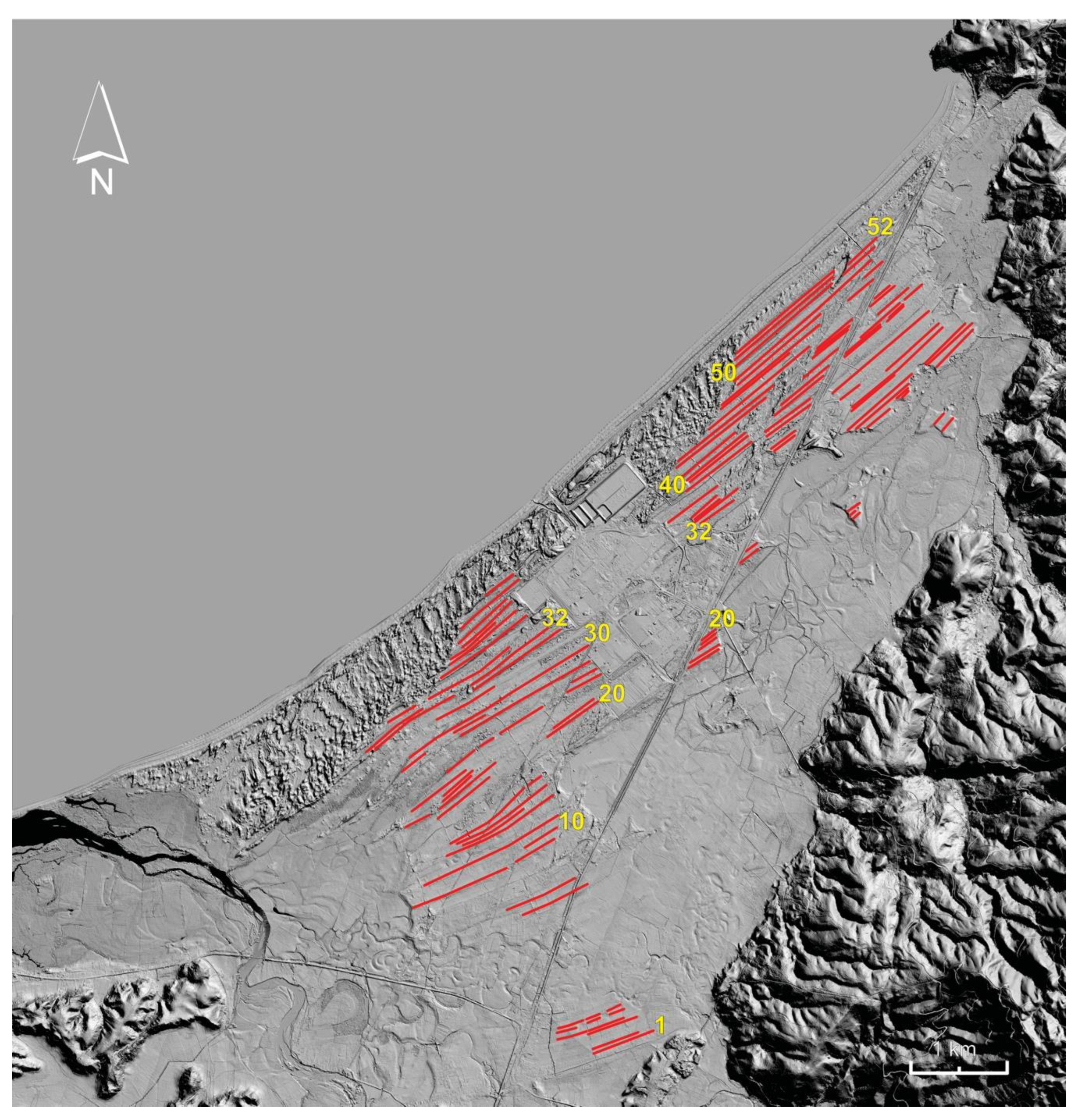
Sequences of beach ridges identified in order of age. The oldest is considered to be Ridge 1, the closest to the marine terrace, and the most recent is Ridge 52, the closest to the coastline. In addition to ridges 1 and 52, ridges 10, 20, 30, 40, and 50 are marked, as well as those that served as a guide for the correlation between lines, specifically ridge 32. It is not ruled out that more ridges were not identified in the count.
Figure A1.
Sequences of beach ridges identified in order of age. The oldest is considered to be Ridge 1, the closest to the marine terrace, and the most recent is Ridge 52, the closest to the coastline. In addition to ridges 1 and 52, ridges 10, 20, 30, 40, and 50 are marked, as well as those that served as a guide for the correlation between lines, specifically ridge 32. It is not ruled out that more ridges were not identified in the count.
Appendix B
Pit
Figure B1.
Pit near the GPR3 profile used to control the data observed in the radargrams.
References
- Roy, P.S.; Cowell, P.J.; Ferland, M.A.; Thom, B.G. Wave-dominated coasts. In Coastal evolution: Late Quaternary shoreline morphodynamics; 1994; pp. 121–186.
- Otvos, E.G. Beach Ridges — Definitions and Significance. Geomorphology 2000, 32, 83–108. [Google Scholar] [CrossRef]
- Neal, A.; Richards, J.; Pye, K. Sedimentology of coarse-clastic beach-ridge deposits, Essex, southeast England. Sediment Geol 2003, 162, 167–198. [Google Scholar] [CrossRef]
- Kinsela, M.A.; Daley, M.J.A.; Cowell, P.J. Origins of Holocene Coastal Strandplains in Southeast Australia: Shoreface Sand Supply Driven by Disequilibrium Morphology. Mar Geol 2016, 374, 14–30. [Google Scholar] [CrossRef]
- Dillenburg, S.R.; Hesp, P.A. Geology and Geomorphology of Holocene Coastal Barriers of Brazil; Springer Science & Business Media; Vol. 107;
- Oliver, T.S.N.; Tamura, T.; Brooke, B.P.; Short, A.D.; Kinsela, M.A.; Woodroffe, C.D.; Thom, B.G. Holocene Evolution of the Wave-Dominated Embayed Moruya Coastline, Southeastern Australia: Sediment Sources, Transport Rates and Alongshore Interconnectivity. Quat Sci Rev 2020, 247, 106566. [Google Scholar] [CrossRef]
- FitzGerald, D.M.; Cleary, W.J.; Buynevich, I. V; Hein, C.J.; Klein, A.H.F.; Asp, N.; Angulo, R. Strandplain Evolution along the Southern Coast of Santa Catarina, Brazil. J Coast Res 2007, 152–156. [Google Scholar]
- Woodroffe, C.D. Coasts: form, process and evolution; Cambridge University Press.
- Scheffers, A.; Engel, M.; Scheffers, S.; Squire, P.; Kelletat, D. Beach Ridge Systems – Archives for Holocene Coastal Events? Progress in Physical Geography: Earth and Environment 2012, 36, 5–37. [Google Scholar] [CrossRef]
- Nelson, A.R.; Manley, W.F. Holocene Coseismic and Aseismic Uplift of Isla Mocha, South-Central Chile. Quaternary International 1992, 15, 61–76. [Google Scholar] [CrossRef]
- Monecke, K.; Templeton, C.K.; Finger, W.; Houston, B.; Luthi, S.; McAdoo, B.G.; Sudrajat, S.U. Beach Ridge Patterns in West Aceh, Indonesia, and Their Response to Large Earthquakes along the Northern Sunda Trench. Quat Sci Rev 2015, 113, 159–170. [Google Scholar]
- Aedo, D.; Melnick, D.; Cisternas, M.; Brill, D. Tectonic Control on Great Earthquake Periodicity in South-Central Chile. Commun Earth Environ 2024, 5, 703. [Google Scholar]
- Tamura, T. Beach Ridges and Prograded Beach Deposits as Palaeoenvironment Records. Earth Sci Rev 2012, 114, 279–297. [Google Scholar] [CrossRef]
- Hede, M.U.; Bendixen, M.; Clemmensen, L.B.; Kroon, A.; Nielsen, L. Joint Interpretation of Beach-Ridge Architecture and Coastal Topography Show the Validity of Sea-Level Markers Observed in Ground-Penetrating Radar Data. Holocene 2013, 23, 1238–1246. [Google Scholar] [CrossRef]
- Silva, A.P.; Klein, A.H.F.; Fetter-Filho, A.F.H.; Hein, C.J.; Méndez, F.J.; Broggio, M.F.; Dalinghaus, C. Climate-Induced Variability in South Atlantic Wave Direction over the Past Three Millennia. Sci Rep 2020, 10, 18553. [Google Scholar] [CrossRef] [PubMed]
- FRASER, C.; HILL, P.R.; ALLARD, M. Morphology and Facies Architecture of a Falling Sea Level Strandplain, Umiujaq, Hudson Bay, Canada. Sedimentology 2005, 52, 141–160. [Google Scholar] [CrossRef]
- HEIN, C.J.; FitzGERALD, D.M.; CLEARY, W.J.; ALBERNAZ, M.B.; De MENEZES, J.T.; KLEIN, A.H. da F. Evidence for a Transgressive Barrier within a Regressive Strandplain System: Implications for Complex Coastal Response to Environmental Change. Sedimentology 2013, 60, 469–502. [Google Scholar] [CrossRef]
- Dillenburg, S.R.; Barboza, E.G.; Rosa, M.L.C.C.; Caron, F.; Sawakuchi, A.O. The Complex Prograded Cassino Barrier in Southern Brazil: Geological and Morphological Evolution and Records of Climatic, Oceanographic and Sea-Level Changes in the Last 7–6 Ka. Mar Geol 2017, 390, 106–119. [Google Scholar] [CrossRef]
- Kelsey, H.M.; Witter, R.C.; Engelhart, S.E.; Briggs, R.; Nelson, A.; Haeussler, P.; Corbett, D.R. Beach Ridges as Paleoseismic Indicators of Abrupt Coastal Subsidence during Subduction Zone Earthquakes, and Implications for Alaska-Aleutian Subduction Zone Paleoseismology, Southeast Coast of the Kenai Peninsula, Alaska. Quat Sci Rev 2015, 113, 147–158. [Google Scholar] [CrossRef]
- Pitman, S.J.; Jol, H.M.; Shulmeister, J.; Hart, D.E. Storm Response of a Mixed Sand Gravel Beach Ridge Plain under Falling Relative Sea Levels: A Stratigraphic Investigation Using Ground Penetrating Radar. Earth Surf Process Landf 2019, 44, 1610–1617. [Google Scholar] [CrossRef]
- Prasad, P.; Loveson, V.J.; Kumar, V.; Shukla, A.D.; Chandra, P.; Verma, S.; Yadav, R.; Magotra, R.; Tirodkar, G.M. Reconstruction of Holocene Relative Sea-Level from Beach Ridges of the Central West Coast of India Using GPR and OSL Dating. Geomorphology 2023, 442, 108914. [Google Scholar] [CrossRef]
- Aedo, D.; Cisternas, M.; Melnick, D.; Esparza, C.; Winckler, P.; Saldaña, B. Decadal Coastal Evolution Spanning the 2010 Maule Earthquake at Isla Santa Maria, Chile: Framing Darwin’s Accounts of Uplift over a Seismic Cycle. Earth Surf Process Landf 2023, 48, 2319–2333. [Google Scholar] [CrossRef]
- Nielsen, L.; Clemmensen, L.B. Sea-level Markers Identified in Ground-penetrating Radar Data Collected across a Modern Beach Ridge System in a Microtidal Regime. Terra Nova 2009, 21, 474–479. [Google Scholar] [CrossRef]
- Clemmensen, L.B.; Nielsen, L. Internal Architecture of a Raised Beach Ridge System (Anholt, Denmark) Resolved by Ground-Penetrating Radar Investigations. Sediment Geol 2010, 223, 281–290. [Google Scholar] [CrossRef]
- Costas, S.; Ferreira, Ó.; Plomaritis, T.A.; Leorri, E. Coastal Barrier Stratigraphy for Holocene High-Resolution Sea-Level Reconstruction. Sci Rep 2016, 6, 38726. [Google Scholar] [CrossRef]
- da Rocha, T.B.; Fernandez, G.B.; de Oliveira Peixoto, M.N. Applications of Ground-Penetrating Radar to Investigate the Quaternary Evolution of the South Part of the Paraiba Do Sul River Delta (Rio de Janeiro, Brazil). J Coast Res 2013, 65, 570–575. [Google Scholar] [CrossRef]
- Pinegina, T.K.; Bourgeois, J.; Bazanova, L.I.; Zelenin, E.A.; Krasheninnikov, S.P.; Portnyagin, M. V Coseismic Coastal Subsidence Associated with Unusually Wide Rupture of Prehistoric Earthquakes on the Kamchatka Subduction Zone: A Record in Buried Erosional Scarps and Tsunami Deposits. Quat Sci Rev 2020, 233, 106171. [Google Scholar] [CrossRef]
- Rodríguez-Santalla, I.; Gomez-Ortiz, D.; Martín-Crespo, T.; Sánchez, M.J.; Montoya-Montes, I.; Martín-Velázquez, S.; Barrio, F.; Serra, J.; Ramírez-Cuesta, J.M.; Gracia, F.J. Study and Evolution of the Dune Field of La Banya Spit in Ebro Delta (Spain) Using LiDAR Data and GPR. Remote Sensing 2021, Vol. 13, Page 802 2021, 13, 802. [Google Scholar] [CrossRef]
- Brooke, B.P.; Huang, Z.; Nicholas, W.A.; Oliver, T.S.N.; Tamura, T.; Woodroffe, C.D.; Nichol, S.L. Relative Sea-Level Records Preserved in Holocene Beach-Ridge Strandplains – An Example from Tropical Northeastern Australia. Mar Geol 2019, 411, 107–118. [Google Scholar] [CrossRef]
- Ciarletta, D.J.; Shawler, J.L.; Tenebruso, C.; Hein, C.J.; Lorenzo-Trueba, J. Reconstructing Coastal Sediment Budgets From Beach- and Foredune-Ridge Morphology: A Coupled Field and Modeling Approach. J Geophys Res Earth Surf 2019, 124, 1398–1416. [Google Scholar] [CrossRef]
- Tamura, T.; Oliver, T.S.N.; Cunningham, A.C.; Woodroffe, C.D. Recurrence of Extreme Coastal Erosion in SE Australia Beyond Historical Timescales Inferred From Beach Ridge Morphostratigraphy. Geophys Res Lett 2019, 46, 4705–4714. [Google Scholar] [CrossRef]
- Switzer, A.D.; Gouramanis, C.; Bristow, C.S.; Simms, A.R. Ground-Penetrating Radar (GPR) in Coastal Hazard Studies. In Geological Records of Tsunamis and other Extreme Waves; Elsevier, 2020; pp. 143–168.
- Doyle, T.B.; Woodroffe, C.D. The Application of LiDAR to Investigate Foredune Morphology and Vegetation. Geomorphology 2018, 303, 106–121. [Google Scholar] [CrossRef]
- Olsen, M.J.; Young, A.P.; Ashford, S.A. TopCAT—Topographical Compartment Analysis Tool to Analyze Seacliff and Beach Change in GIS. Comput Geosci 2012, 45, 284–292. [Google Scholar] [CrossRef]
- Angermann, D.; Klotz, J.; Reigber, C. Space-Geodetic Estimation of the Nazca-South America Euler Vector. Earth Planet Sci Lett 171, 329–334.
- Davis, R.A. 10.16 Evolution of Coastal Landforms. Treatise on Geomorphology 2013, 10, 417–448. [Google Scholar] [CrossRef]
- Araya-Vergara, J.F. Análisis de La Localización de Los Procesos y Formas Predominantes de La Linea Litoral de Chile: Observación Preliminar. Investigaciones Geográficas: Una mirada desde el sur 1982, 29, g–35. [Google Scholar] [CrossRef]
- Isla, M.F.; Moyano-Paz, D.; FitzGerald, D.M.; Simontacchi, L.; Veiga, G.D. Contrasting Beach-Ridge Systems in Different Types of Coastal Settings. Earth Surf Process Landf 2023, 48, 47–71. [Google Scholar] [CrossRef]
- Isla, F.I.; Flory, J.Q.; Martínez, C.; Fernández, A.; Jaque, E. The evolution of the bío bío delta and the coastal plains of the Arauco Gulf, bío bío region: the holocene sea-level Curve of Chile. J Coast Res 2012, 28, 102–111. [Google Scholar] [CrossRef]
- Jara-Muñoz, J.; Melnick, D.; Zambrano, P.; Rietbrock, A.; González, J.; Argandoña, B.; Strecker, M.R. Quantifying Offshore Fore-arc Deformation and Splay-fault Slip Using Drowned Pleistocene Shorelines, Arauco Bay, Chile. J Geophys Res Solid Earth 2017, 122, 4529–4558. [Google Scholar] [CrossRef]
- Melnick, D.; Bookhagen, B.; Strecker, M.R.; Echtler, H.P. Segmentation of Megathrust Rupture Zones from Fore-arc Deformation Patterns over Hundreds to Millions of Years, Arauco Peninsula, Chile. J Geophys Res Solid Earth 2009, 114. [Google Scholar] [CrossRef]
- Garrett, E.; Melnick, D.; Dura, T.; Cisternas, M.; Ely, L.L.; Wesson, R.L.; Whitehouse, P.L. Holocene Relative Sea-Level Change along the Tectonically Active Chilean Coast. Quat Sci Rev 2020, 236, 106281. [Google Scholar]
- Winckler, P.; Martín, R.A.; Esparza, C.; Melo, O.; Sactic, M.I.; Martínez, C. Projections of Beach Erosion and Associated Costs in Chile. Sustainability (Switzerland) 2023, 15. [Google Scholar] [CrossRef]
- Schoener, G.; Muñoz, E.; Arumí, J.L.; Stone, M.C. Impacts of Climate Change Induced Sea Level Rise, Flow Increase and Vegetation Encroachment on Flood Hazard in the Biobío River, Chile. Water (Switzerland) 2022, 14. [Google Scholar] [CrossRef]
- Lamy, F.; Hebbeln, D.; Wefer, G. High-Resolution Marine Record of Climatic Change in Mid-Latitude Chile during the Last 28,000 Years Based on Terrigenous Sediment Parameters. Quat Res 1999, 51, 83–93. [Google Scholar] [CrossRef]
- Lamy, F.; Hebbeln, D.; Röhl, U.; Wefer, G. Holocene Rainfall Variability in Southern Chile: A Marine Record of Latitudinal Shifts of the Southern Westerlies. Earth Planet Sci Lett 2001, 185, 369–382. [Google Scholar] [CrossRef]
- Jenny, B.; Valero-Garcés, B.L.; Urrutia, R.; Kelts, K.; Veit, H.; Appleby, P.G.; Geyh, M. Moisture Changes and Fluctuations of the Westerlies in Mediterranean Central Chile during the Last 2000 Years: The Laguna Aculeo Record (33 50′ S. Quaternary International 2002, 87, 3–18. [Google Scholar] [CrossRef]
- Villa-Martínez, R.; Villagrán, C.; Jenny, B. The Last 7500 Cal Yr BP of Westerly Rainfall in Central Chile Inferred from a High-Resolution Pollen Record from Laguna Aculeo. Quat Res 2003, 60, 284–293. [Google Scholar] [CrossRef]
- Sterken, M.; Verleyen, E.; Sabbe, K.; Terryn, G.; Charlet, F.; Bertrand, S.; Vyverman, W. Late Quaternary Climatic Changes in Southern Chile, as Recorded in a Diatom Sequence of Lago Puyehue (40 40′ S. J Paleolimnol 2008, 39, 219–235. [Google Scholar] [CrossRef]
- Frugone-Álvarez, M.; Latorre, C.; Giralt, S.; Polanco-Martínez, J.; Bernárdez, P.; Oliva-Urcia, B.; Valero-Garcés, B. A 7000-year High-resolution Lake Sediment Record from Coastal Central Chile (Lago Vichuquén, 34° S): Implications for Past Sea Level and Environmental Variability. J Quat Sci 2017, 32, 830–844. [Google Scholar]
- Francois, J.P.; Hernandez, P.; Schneider, I.; Cerda, J. Nuevos datos en torno a la historia paleoambiental del centro-sur de Chile. El registro sedimentario y palinológico del Humedal Laguna Verde (36°47’S), Península Hualpén, Región del Bío-Bío, Chile. Revista De Geografía Norte Grande 2024. [Google Scholar] [CrossRef]
- Lamy, F.; Kilian, R.; Arz, H.W.; Francois, J.P.; Kaiser, J.; Prange, M.; Steinke, T. Holocene Changes in the Position and Intensity of the Southern Westerly Wind Belt. Nat Geosci 2010, 3, 695–699. [Google Scholar]
- Moreno, M.; Melnick, D.; Rosenau, M.; Baez, J.; Klotz, J.; Oncken, O.; Hase, H. Toward Understanding Tectonic Control on the Mw 8.8 2010 Maule Chile Earthquake. Earth Planet Sci Lett 2012, 321, 152–165. [Google Scholar] [CrossRef]
- Lin, Y.N.N.; Sladen, A.; Ortega-Culaciati, F.; Simons, M.; Avouac, J.P.; Fielding, E.J.; Socquet, A. Coseismic and Postseismic Slip Associated with the 2010 Maule Earthquake, Chile: Characterizing the Arauco Peninsula Barrier Effect. J Geophys Res Solid Earth 2013, 118, 3142–3159. [Google Scholar] [CrossRef]
- Melnick, D.; Cisternas, M.; Moreno, M.; Norambuena, R. Estimating Coseismic Coastal Uplift with an Intertidal Mussel: Calibration for the 2010 Maule Chile Earthquake (Mw= 8.8. Quat Sci Rev 2012, 42, 29–42. [Google Scholar]
- Quezada, J.; Jaque, E.; Fernández, A.; Vásquez, D. Cambios en el relieve generados como consecuencia del terremoto Mw= 8,8 del 27 de febrero de 2010 en el centro-sur de Chile. Revista de Geografía Norte Grande 2012, 53, 35–55. [Google Scholar]
- Martínez, C.; Rojas, D.; Quezada, M.; Quezada, J.; Oliva, R. Post-Earthquake Coastal Evolution and Recovery of an Embayed Beach in Central-Southern Chile. Geomorphology 2015, 250, 321–333. [Google Scholar]
- Cisternas, M.; Melnick, D.; Ely, L.; Wesson, R.; Norambuena, R. Similarities between the Great Chilean Earthquakes of 1835 and 2010. In Proceedings of the Chapman Conference on Giant Earthquakes and their Tsunamis, AGU; 2010; Vol. 19.
- Moreno, M.; Rosenau, M.; Oncken, O. 2010 Maule Earthquake Slip Correlates with Pre-Seismic Locking of Andean Subduction Zone. Nature 2010, 467, 198–202. [Google Scholar]
- Fitzroy, R. Narrative of the Surveying Voyages of His Majesty’s Ships Adventure and Beagle Between the Years 1826 and 1836: Describing Their Examination of the Southern Shores of South America. In Proceedings of the and the Beagle’s Circumnavigation of the Globe: Proceedings of the Second Expedition; 1839.
- Giorgini, E.; Orellana, F.; Arratia, C.; Tavasci, L.; Montalva, G.; Moreno, M.; Gandolfi, S. InSAR Monitoring Using Persistent Scatterer Interferometry (PSI) and Small Baseline Subset (SBAS) Techniques for Ground Deformation Measurement in Metropolitan Area of Concepción, Chile. Remote Sens (Basel) 2023, 15. [Google Scholar] [CrossRef]
- Wesson, R.L.; Melnick, D.; Cisternas, M.; Moreno, M.; Ely, L.L. Vertical Deformation through a Complete Seismic Cycle at Isla Santa María, Chile. Nat Geosci 2015, 8, 547–551. [Google Scholar]
- Villagrán, M.; Gómez, M.; Martínez, C. Coastal Erosion and a Characterization of the Morphological Dynamics of Arauco Gulf Beaches under Dominant Wave Conditions. Water (Switzerland) 2023, 15. [Google Scholar] [CrossRef]
- Tzanis, A. MATGPR Release 2: A Freeware MATLAB ® Package for the Analysis & Interpretation of Common & Single Offset GPR Data. Geophysical Research Abstracts 2010, 17–43. [Google Scholar]
- Bristow, C.S.; Neil Chroston, P.; Bailey, S.D. The Structure and Development of Foredunes on a Locally Prograding Coast: Insights from Ground-Penetrating Radar Surveys, Norfolk, UK. Sedimentology 2000, 47, 923–944. [Google Scholar] [CrossRef]
- Oliver, T.S.; Dougherty, A.J.; Gliganic, L.A.; Woodroffe, C.D. Towards More Robust Chronologies of Coastal Progradation: Optically Stimulated Luminescence Ages for the Coastal Plain at Moruya, South-Eastern Australia. 2014, 25, 536–546. [Google Scholar] [CrossRef]
- Hein, C.J.; Fitzgerald, D.M.; De Souza, L.H.P.; Georgiou, I.Y.; Buynevich, I. V.; Klein, A.H.D.F.; De Menezes, J.T.; Cleary, W.J.; Scolaro, T.L. Complex Coastal Change in Response to Autogenic Basin Infilling: An Example from a Sub-Tropical Holocene Strandplain. Sedimentology 2016, 63, 1362–1395. [Google Scholar] [CrossRef]
- Brooke, B.P.; Huang, Z.; Nicholas, W.A.; Oliver, T.S.N.; Tamura, T.; Woodroffe, C.D.; Nichol, S.L. Relative Sea-Level Records Preserved in Holocene Beach-Ridge Strandplains – An Example from Tropical Northeastern Australia. Mar Geol 2019, 411, 107–118. [Google Scholar] [CrossRef]
- Ribolini, A.; Bertoni, D.; Bini, M.; Sarti, G. Ground-Penetrating Radar Prospections to Image the Inner Structure of Coastal Dunes at Sites Characterized by Erosion and Accretion (Northern Tuscany, Italy. Applied Sciences 2021, 11, 11260. [Google Scholar]
- Rodríguez-Santalla, I.; Gomez-Ortiz, D.; Martín-Crespo, T.; Sánchez, M.J.; Montoya-Montes, I.; Martín-Velázquez, S.; Barrio, F.; Serra, J.; Ramírez-Cuesta, J.M.; Gracia, F.J. Study and Evolution of the Dune Field of La Banya Spit in Ebro Delta (Spain) Using Lidar Data and Gpr. Remote Sens (Basel) 2021, 13, 1–17. [Google Scholar] [CrossRef]
- Silva Figueiredo, M.; Rocha, T.; Brill, D.; Borges Fernandez, G. Morphostratigraphy of Barrier Spits and Beach Ridges at the East Margin of Salgada Lagoon (Southeast Brazil. J South Am Earth Sci 2022, 116, 103850. [Google Scholar]
- Prasad, P.; Loveson, V.J.; Kumar, V.; Shukla, A.D.; Chandra, P.; Verma, S.; Yadav, R.; Magotra, R.; Tirodkar, G.M. Reconstruction of Holocene Relative Sea-Level from Beach Ridges of the Central West Coast of India Using GPR and OSL Dating. Geomorphology 2023, 442. [Google Scholar] [CrossRef]
- Fanucci, F.; Amore, C.; Pineda, V. Characteristics and Dynamics of the Coasts in the Araugo Gulf (Central Chile). In Proceedings of the Bollettino di oceanologia teorica ed applicata; 1992; Vol. 10, pp. 265–271. 1992; Vol. 10.
- Flores-Aqueveque, V.; Arias, P.A.; Gómez-Fontealba, C.; González-Arango, C.; Apaestegui, J.; Evangelista, H.; Guerra, L.; Latorre, C. The South American Climate During the Last Two Millennia. In Oxford Research Encyclopedia of Climate Science; Oxford University Press, 2024.
- Hein, C.J.; Fitzgerald, D.M.; Cleary, W.J.; Albernaz, M.B.; De Menezes, J.T.; Klein, A.H. da F. Evidence for a Transgressive Barrier within a Regressive Strandplain System: Implications for Complex Coastal Response to Environmental Change. Sedimentology 2013, 60, 469–502. [Google Scholar] [CrossRef]
- Pye, K.; Tsoar, H. Aeolian Sand and Sand Dunes. Aeolian Sand and Sand Dunes 2009. [Google Scholar] [CrossRef]
- Albert, F. Las dunas del centro de Chile. Edición de la Pontifica Universidad Católica de Chile; Biblioteca Fundamentos de la Construcción de Chile: Santiago, Chile, 1900. [Google Scholar]
- Bertrand, S.; Boës, X.; Castiaux, J.; Charlet, F.; Urrutia, R.; Espinoza, C.; Fagel, N. Temporal Evolution of Sediment Supply in Lago Puyehue (Southern Chile) during the Last 600 Yr and Its Climatic Significance. Quat Res 2005, 64, 163–175. [Google Scholar]
- Lamy, F.; Kaiser, J.; Lamy, F. Glacial to Holocene Paleoceanographic and Continental Paleoclimate Reconstructions Based on ODP Site 1233/GeoB 3313 Off Southern Chile. 2009, 129–156. [CrossRef]
Figure 1.
Study area. (a) The tectonic context of Chile faces a subduction zone between the Nazca and South American plates. (b) Rupture and slip area of the 2010 Mw 8.8 earthquake. Note the 10 m slip in the Gulf of Arauco. (c) A red box indicates the coast facing the Gulf of Arauco, which functions as a complex geomorphological system of which the LCS is part, whose location is indicated in the orange square (detail in Figure 2).
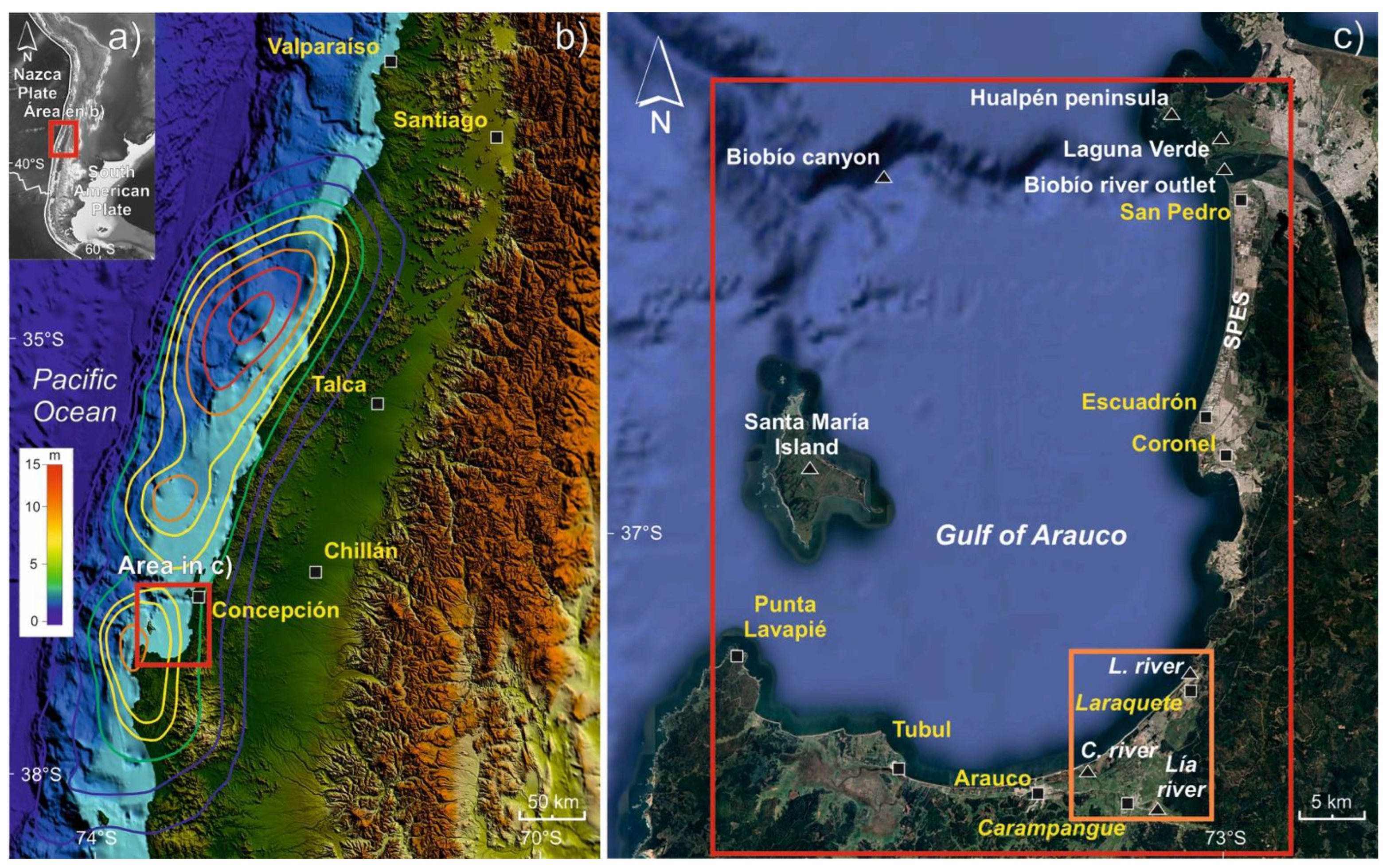
Figure 2.
DTM of LCS obtained from LiDAR data. Red arrows indicate patches of strandplain eroded by past fluvial activity. Yellow arrows indicate oxbows. Orange arrows indicate areas where vegetated dune fields cover beach ridges. Red lines represent GPR profiles.
Figure 2.
DTM of LCS obtained from LiDAR data. Red arrows indicate patches of strandplain eroded by past fluvial activity. Yellow arrows indicate oxbows. Orange arrows indicate areas where vegetated dune fields cover beach ridges. Red lines represent GPR profiles.
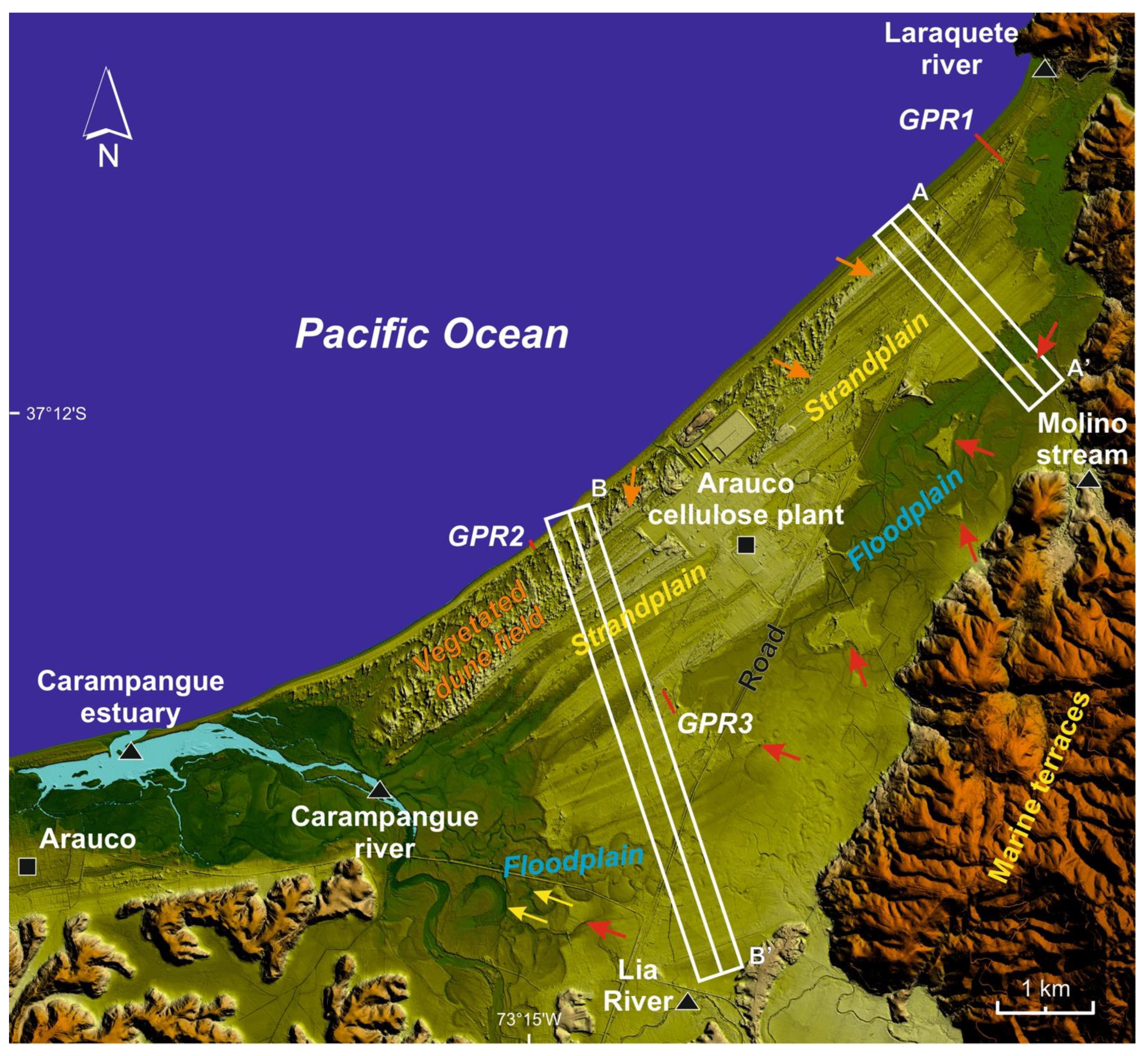
Figure 3.
Swath profiles (500 m wide) of the LCS. Their location is shown in Figure 2.
Figure 3.
Swath profiles (500 m wide) of the LCS. Their location is shown in Figure 2.
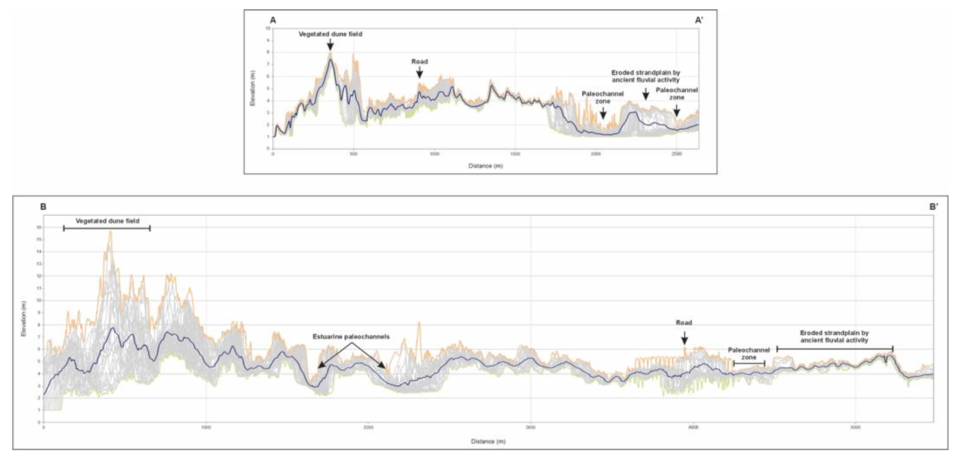
Figure 5.
GPR1 profile. In (a), the facies interpretation is shown in colors and with legends. In (b), the green arrows show pre-earthquake and 2023 runnels. Like a shoreface, this runnel and other beach structures are buried under a sand sheet and associated with a SWZ (planiform and/or convex reflectors). In 2023, another runnel was formed, showing the same structural characteristics as the pre-earthquake runnel (planiform and/or convex reflectors). In (c), the location of the GPR profile over the vegetated dunes and the paleochannel zone.
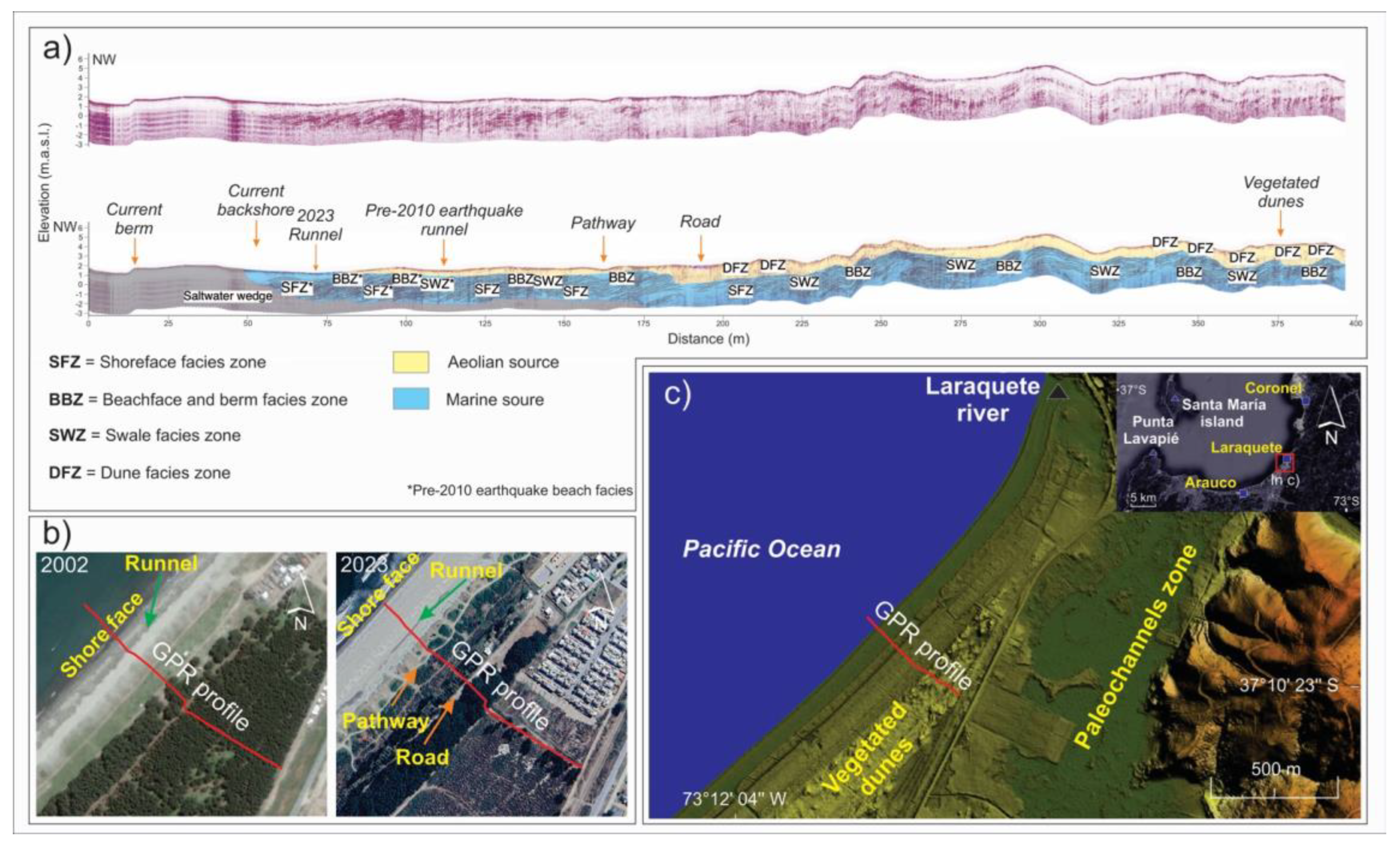
Figure 6.
GPR2 profile. In (a), the facies are shown in colors and with legends. In (b), the location of the shoreface before the earthquake and in 2023. A change in the location of the shoreface and the extension of the beach was caused by the 2010 earthquake, and sand sheets covered the pre-earthquake beach structures. In (c), the location of the GPR line concerning the vegetated dunes and the strandplain.
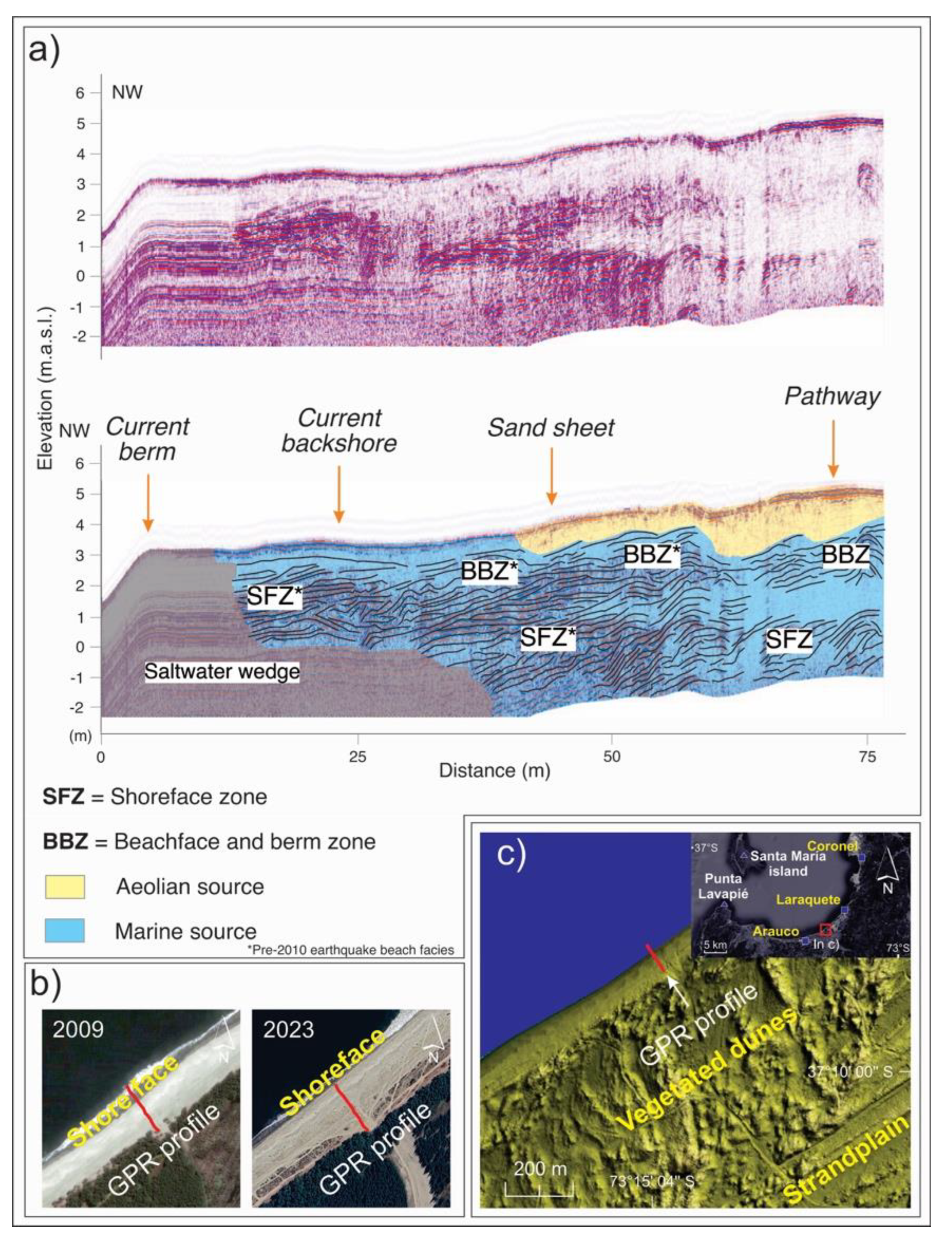
Figure 7.
GPR3 profile. In (a), the letters R (1,2 and 3) are interpreted as beach ridges covered by aeolian features, while the letters S (1, 2, and 3) are interpreted as swales or depressions between ridges. In (b), the location of the GPR line over the vegetated dunes and the strandplain. The light blue dot represents the location of the pit visible in Figure B1.
Disclaimer/Publisher’s Note: The statements, opinions and data contained in all publications are solely those of the individual author(s) and contributor(s) and not of MDPI and/or the editor(s). MDPI and/or the editor(s) disclaim responsibility for any injury to people or property resulting from any ideas, methods, instructions or products referred to in the content. |
© 2025 by the authors. Licensee MDPI, Basel, Switzerland. This article is an open access article distributed under the terms and conditions of the Creative Commons Attribution (CC BY) license (http://creativecommons.org/licenses/by/4.0/).
Copyright: This open access article is published under a Creative Commons CC BY 4.0 license, which permit the free download, distribution, and reuse, provided that the author and preprint are cited in any reuse.


