
Submitted:
23 March 2025
Posted:
26 March 2025
You are already at the latest version
Abstract
Vehicle accidents, particularly passenger vehicle-to-passenger vehicle (PV-PV) collisions, cause significant property damage and driver injuries, resulting in substantial economic losses and health risks. Most existing studies focus on macro-level predictions, such as accident frequency, but lack detailed collision-level analysis, which limits precise severity prediction. This study investigates various accident-related factors, including environmental conditions, vehicle attributes, driver characteristics, pre-crash scenarios, and collision dynamics.Using data from the National Highway Traffic Safety Administration’s (NHTSA) Crash Report Sampling System (CRSS) and Fatality Analysis Reporting System (FARS), the dataset was balanced by integrating complementary severity-level data with random over-sampling and under-sampling techniques. The Minimum Redundancy Maximum Relevance (mRMR) algorithm was used for feature selection to minimize redundancy and identify key features.Five advanced machine learning models were employed for severity prediction, with Extreme Gradient Boosting (XGBoost) achieving the best performance: 84.9% accuracy, 84.85% precision, 84.90% recall, and an F1-score of 84.87%. SHapley Additive exPlanations (SHAP) analysis was employed to interpret the model and conduct a deep analysis of accident features, including feature importance, dependencies, and their combined effects on severity prediction.The findings highlight the effectiveness of interpretable machine learning in understanding accident severity and identifying key factors influencing driver injuries.
Keywords:
explainable machine learning
; driver injury severity prediction
; accident datasets
; feature extraction
; accident feature analysis
; SHAP
1. Introduction
Passenger vehicles (PVs), as motor vehicles designed to transport people and their belongings, have significantly enhanced the convenience of human mobility [1,2,3]. PVs are primarily categorized into two major groups: passenger cars and light trucks [4]. Among various vehicle types, PVs not only constitute the majority of the vehicle fleet but also account for the highest proportion of traffic accidents [5]. According to the 2024 analysis conducted by the National Highway Traffic Safety Administration on the 2022 Crash Report Sampling System data [6], more than 64% of police-reported crashes involved two-vehicle collisions, with PV-PV crashes accounting for the highest proportion at 73.4%. Drivers are the most severely affected individuals in traffic accidents, representing 67.7% of all road traffic casualties in 2021. Therefore, understanding the factors influencing collision occurrences and injury severity is crucial for enhancing traffic safety.
PV-PV collisions constitute a complex dynamic process, as illustrated in Figure 1, encompassing dual-vehicle and driver characteristics, environmental conditions, causal factors, and pre-collision and collision dynamics [7]. accident severity prediction and feature analysis involve four key steps [8]: data acquisition, preprocessing, feature selection, and model selection. First, obtaining a reliable and comprehensive accident dataset is foundational [9]. Second, preprocessing steps like outlier removal, missing value imputation, encoding, and balancing ensure data suitability for analysis [10]. Third, feature selection addresses redundancy and enhances prediction performance and interpretability [11]. Finally, selecting an appropriate model tailored to the dataset and research objectives is critical for effective analysis.
Recent studies have focused on identifying and quantifying factors influencing accident injury severity, primarily through statistical methods. For instance, Dongdong Song et al. (2023) utilized a random parameters bivariate probability model to analyze UK truck-car collision data (2017–2019), identifying key factors affecting driver injury severity and proposing safety improvements [12]. Similarly, Hongren Gong et al. (2022) applied a Bayesian multivariate random parameters logit model to U.S. GES and CRSS two-vehicle collision data (2010–2018), uncovering significant associations between factors and injury risk, along with heterogeneity and temporal instability in effects [13]. In another study, Joon-Ki Kim et al. (2013) analyzed California single-vehicle crash data (2003–2004) using a mixed logit model, highlighting the influence of age and gender on injury severity and the presence of heterogeneity [14]. Donald Mathew Cerwick et al. (2014) compared mixed logit and latent class models using multi-vehicle heavy truck crash data from Iowa (2007–2012), finding that while the latent class model fit slightly better, the mixed logit model yielded probability predictions closer to observed values, with similar marginal effects for most variables [15].
Statistical methods have been widely used due to their strong interpretability, aiding in understanding the mechanisms behind accident heterogeneity and severity correlations. However, their dependence on linear assumptions and independence constraints severely limits their ability to model the complex, nonlinear interactions among accident-related factors. [16]. Traffic accidents, as complex systems, involve multiple collinear and higher-order interactions among influencing factors [17,18], such as vehicle dynamics and environmental conditions. The results obtained from traditional methods heavily depend on the validity of their assumptions. If these assumptions deviate from reality—such as neglecting nonlinear interactions—the reliability and generalizability of the analysis are significantly compromised [19,20,21]. In contrast, machine learning (ML) methods excel in nonlinear modeling and can effectively capture intricate relationships among accident features without relying on strict statistical assumptions. They can extract latent patterns from high-dimensional data, substantially improving the accuracy of accident severity prediction [22,23].
In recent years, ML techniques have emerged as a promising alternative to traditional data analysis methods for injury severity analysis, offering the ability to extract valuable insights from large-scale, complex, and heterogeneous datasets. Ensemble machine learning (EML) and deep learning (DL) models are widely used in traffic accident severity prediction, but their applications differ. DL models are mainly used for macroscopic accident analysis, utilizing spatial-temporal data from images, videos, or sequences to predict accident occurrence and severity, aiding traffic management in intervention and emergency response. Yu et al. (2021) developed a Deep Spatio-Temporal Graph Convolutional Network using heterogeneous traffic data in Beijing to improve accident risk prediction, the model enhances prediction accuracy, enabling early warnings of potential hazards and supporting safer route selection [24].Fares Alhaek et al. (2024) proposed a CNN-BiLSTM-based DL method for traffic accident severity prediction. Experiments on UK city data showed it outperformed baselines [25]. However, due to the structured nature of accident severity datasets, Tabular is the most basic form of traffic accident datasets. EML models has demonstrated its superiority in handling datasets with tabular data format. EML’s strength lies in its ability to combine multiple base models, enabling it to capture complex patterns and relationships within the data more effectively than single models. In the field of accident severity prediction, this advantage is particularly evident. For example, various ensemble machine learning models have outperformed other machine learning models. Models like Random Forest [26], XGBoost [27,28], LightGBM [29], CatBoost [30] and AdaBoost [31] are more suitable for microscopic accident severity prediction. These models offer better interpretability, which means it is easier to understand how different factors contribute to accident severity.
EML algorithms improve predictive performance by integrating multiple decision trees. Although a single decision tree offers inherent interpretability, the depth and number of nodes in ensemble models significantly increase in high-dimensional accident feature spaces, leading to excessive model complexity and a notable reduction in interpretability [32]. Despite their superior predictive performance, the "black-box" nature of ensemble models hinders the interpretation of accident causation mechanisms. Explainable ML techniques, SHAP [33], provide a viable solution to this issue. SHAP, based on Shapley values from game theory, quantifies feature contributions and reveals interaction effects. Its additive feature attribution property aligns well with tree-based ensemble models, supporting both global and local interpretability [34]. Widely integrated with ensemble machine learning, SHAP has become a preferred tool for analyzing the relationship between accident severity and contributing factors, offering a new paradigm for passenger vehicle collision analysis. It not only ensures the accuracy of the prediction model but also enables in - depth interpretation of the model and feature analysis.
Current research on accident severity prediction faces several challenges. First, natural accident datasets suffer from severe class imbalance [6,12,13], where fatal accident cases are significantly underrepresented compared to non-injury cases. This imbalance poses challenges for traditional resampling methods in effectively balancing severity levels [35]. Moreover, accident datasets often contain a mix of categorical and numerical features, which limits the applicability of Euclidean distance-based oversampling techniques such as Synthetic Minority Over-sampling Technique (SMOTE) [36]. Thus, addressing data imbalance at the data collection stage is crucial. Second, existing studies primarily rely on empirical heuristics for feature selection [12], lacking rigorous scientific justification. Consequently, the representativeness and rationality of selected features remain inadequately explained.
To address the issue of class imbalance in accident severity datasets, this study first integrates the CRSS and FARS datasets from the NHTSA. This integration reduces the severity imbalance ratio from 175.1 in CRSS and 10.2 in FARS to 5.1 in the combined dataset. Furthermore, a combination of oversampling and undersampling techniques is employed to achieve a balanced distribution of severity categories. For feature selection, traditional methods often rely on Pearson correlation coefficients to eliminate highly correlated and irrelevant variables. However, this approach is not suitable for accident datasets dominated by categorical features, as categorical values represent discrete labels rather than numerical relationships. o enhance the rationality of feature extraction, this study adopts the mRMR algorithm based on mutual information [37]. This algorithm has been widely applied in Disease Diagnosis [38,39]. Compared with other feature extraction methods, it demonstrates the best performance while requiring the fewest number of features [40]. Subsequently, this study applies ensemble machine learning algorithms—including CatBoost, AdaBoost, XGBoost, Random Tree, LightGBM, and decision trees—to accident severity prediction. By comparing the predictive performance of different models, the best-performing model is selected for SHAP-based interpretability analysis, facilitating insights into feature importance and improving the explainability of accident severity predictions.
The contributions of this paper can be summarized as follows:
(1) Integrated two distinct accident datasets to address imbalance issues and applied the mRMR algorithm for key feature extraction, reducing redundancy and improving model accuracy across all severity levels.
(2) Proposed a novel micro-level analytical approach for PV-PV accidents, incorporating dual-vehicle factors to simultaneously enhance prediction accuracy and model interpretability, advancing beyond traditional macro-level methods.
(3) Performed a systematic evaluation of state-of-the-art EML models for PV-PV accident severity prediction and integrated the optimal ensemble model with SHAP interpretation, enabling comprehensive feature analysis and addressing a critical research gap in traffic safety analytics.
The remainder of this paper is organized as follows. Section 2 describes the methodologies, encompassing data preprocessing techniques, feature extraction methods, predictive modeling approaches, and explainable AI algorithms. Section 3 presents the dataset’s statistical characteristics and feature analysis. Section 4 details the experimental results, including model performance evaluation and critical factor analysis. Section 5 discusses the research implications and study limitations. Finally, Section 6 concludes the paper and proposes future research directions.
2. Methods
The technical route of this study is shown in Figure 2, which is mainly divided into three parts: the first part is data collection and preprocessing, which aims to provide a structured data set that meets research needs to improve the accuracy and reliability of the model; the second part is model training and tuning, which aims to improve the predictive performance and generalization ability of the model by optimizing model parameters; the third part is to interpret and analyze the characteristics of the optimal model to reveal the key factors behind the model decision and enhance the interpretability and transparency of the model.
2.1. Accident Data Collection and Preprocessing
2.1.1. Accident Data Collection
In accident severity prediction research, class imbalance is a common issue, particularly due to the relatively low number of fatal accident samples, which limits models’ ability to predict severe accidents. Additionally, these datasets typically contain both categorical and numerical features, making traditional Euclidean distance-based SMOTE algorithms less effective for data balancing. To address dataset imbalance, this study integrates two complementary NHTSA datasets: CRSS and FARS. The FARS dataset, containing comprehensive fatal accident records, effectively compensates for the scarcity of severe cases in CRSS. This integration enhances the representation of high-severity accidents at the data source level, which improves the model’s predictive accuracy for severe accident classification.
2.1.2. Dataset Preprocessing
1) Dataset Compilation:
The accident-related data are extracted from multiple relational tables within both CRSS and FARS datasets, including accident records, person information, event sequences, and vehicle damage reports. These heterogeneous data sources are consolidated into a unified structured dataset through a systematic integration process. A composite primary key, comprising Accident ID and Driver ID, is implemented to ensure precise data linkage and maintain referential integrity across all integrated tables.
2) Case Selection:
This study focuses on predicting driver injury severity in PV-PV collisions. Accordingly, vehicle collision cases involving exactly two passenger vehicles with corresponding driver characteristics were extracted from the integrated dataset, ensuring alignment with the research focus.
3) Data Cleaning:
Features with excessive missing values were removed. Features with minimal missing values were imputed using a context-based approach. Cases lacking critical information, such as driver injury severity levels, were excluded to ensure data quality.
4) Encoding and Normalization:
Categorical feature encoding in the original dataset was not directly related to injury severity. Although decision tree-based ensemble models are unaffected by encoding order, it influences the interpretability of SHAP-based feature analysis. Therefore, target encoding was applied, ranking categorical features in ascending order based on their mean injury severity levels. Numerical features were standardized to eliminate scale differences, ensuring model stability and convergence. Minor injury categories (e.g., Possible injury and Suspected minor injury) lacked sufficient distinction. Thus, injury severity levels were reclassified as follows:
No apparent injury → Level0
Possible injury & Suspected minor injury → Level1
Suspected serious injury → Level2
Fatal injury → Level3
5) Data Balancing:
The integration of CRSS and FARS inherently mitigated class imbalance. To further balance the dataset, a combination of random oversampling and undersampling was applied [41]. The average sample size across injury severity levels was used as a reference: oversampling was conducted for underrepresented classes, while undersampling was applied to overrepresented classes. To prevent overfitting and enhance model generalization, categorical features remained unchanged during oversampling, whereas numerical features were perturbed by adding random noise in the range of -5% to +5%. The total dataset size remained constant before and after balancing.
2.2. Feature Selection
Feature selection is a crucial step in accident severity prediction, as redundant and irrelevant features can negatively impact model performance. In this study, the mRMR [37] method was employed for feature selection in accident severity prediction. Compared to traditional correlation-based feature selection methods (e.g., Pearson correlation), mRMR is more effective for datasets with categorical features, as it does not assume linear relationships. The mRMR algorithm is a widely used method for selecting an optimal subset of features by balancing two key objectives:
1. Maximum Relevance: The selected features should have the highest relevance to the target variable.
2. Minimum Redundancy: The selected features should be minimally correlated with each other to reduce redundancy.
2.2.1. Mutual Information (MI) Definition
The mutual information quantifies the dependency between two variables X and Y, and is defined as:
where represents the joint probability distribution, and and are the marginal distributions of X and Y, respectively.
2.2.2. Maximum Relevance Criterion
The relevance of a feature set S with respect to the target variable c is computed as the average mutual information between each feature and c:
where is the number of selected features. The goal is to maximize this relevance measure.
2.2.3. Minimum Redundancy Criterion
To ensure that the selected features are not highly correlated with each other, the redundancy term is defined as the average mutual information among selected features:
The goal is to minimize this redundancy measure.
2.2.4. mRMR Optimization Objective
The final objective of mRMR is to simultaneously maximize relevance and minimize redundancy, which can be formulated as:
This ensures that the selected feature subset retains the most informative variables while reducing redundancy.
2.3. Prediction Model
Given the superior EML models in accident severity prediction, this study adopts them as the primary predictive approach. Specifically, five top-performing EML models—Random Forest, LightGBM, XGBoost, CatBoost, and AdaBoost—are selected, with the Decision Tree model serving as the baseline. A brief introduction to the principles and core formulas of each model is provided below.
2.3.1. Decision Tree
A Decision Tree is a tree-structured model for classification and regression [42], which recursively partitions the feature space to construct decision rules. Its core idea is to select the optimal splitting feature based on Information or Impurity.
Information measures the improvement in dataset purity before and after splitting, calculated as:
Where is the entropy of dataset D, and is the subset where feature A takes the value v.
measures the impurity of a dataset, calculated as:
Where is the proportion of samples of the class in dataset D.
2.3.2. Random Forest
Random Forest is an ensemble learning method based on decision trees, designed to enhance generalization by constructing multiple decision trees and aggregating their predictions [43]. Its core principle involves building diverse decision trees using Bootstrap Sampling and Random Feature Selection. For classification tasks, Random Forest determines the final prediction through majority voting:
Where is the prediction of the decision tree, and T is the number of trees.
2.3.3. LightGBM
LightGBM is an efficient implementation of Gradient Boosting Trees that leverages histogram-based decision tree algorithms and Gradient-based One-Side Sampling (GOSS) to accelerate training [44]. The objective function of LightGBM consists of a loss function and a regularization term:
Where is the loss function, and is the complexity regularization term for the k-th tree.
2.3.4. XGBoost
XGBoost is a high-performance algorithm based on Gradient Boosting Trees [45], which improves model accuracy by using a second-order Taylor expansion to approximate the objective function and introduces regularization terms to prevent overfitting. The objective function of XGBoost is:
Where is the number of leaf nodes in the k-th tree, represents the vector of leaf node weights in the k-th tree, and and are regularization coefficients. The term is the L2 norm (squared) of the leaf node weights, serving as a regularization to penalize large weights and reduce model complexity, thus preventing overfitting.
2.3.5. CatBoost
CatBoost is a gradient boosting algorithm optimized for categorical features [46], which processes them using Target Statistics for encoding and Ordered Boosting to prevent target leakage. For a categorical feature x, CatBoost encodes it using Target Statistics as follows:
where a is a smoothing parameter to control the impact of prior knowledge, and p is the global mean target value. The term is an indicator function that equals 1 if , and 0 otherwise.
2.3.6. AdaBoost
AdaBoost is an ensemble learning method based on weighted voting [47], which iteratively adjusts the sample weights to train multiple weak classifiers and aggregates their predictions. In the t-th iteration, the sample weights are updated as follows:
where is the weight of sample i in the -th iteration, is the weight of sample i in the t-th iteration, is the weight of the t-th weak classifier, is the true label of sample i (with values ), and is the prediction of the t-th weak classifier for sample . The weight of the weak classifier is computed as
where represents the error rate of the weak classifier in the t-th iteration.
2.4. Model Interpretation and Feature Analysis
SHAP is a unified framework for interpreting machine learning models by assigning each feature a contribution value based on its impact on the model’s prediction [48]. It is rooted in cooperative game theory and Shapley values, ensuring fair and consistent feature attribution. SHAP offers several key advantages: Additivity: SHAP values decompose the model’s prediction into the sum of contributions from each feature, providing a clear and interpretable explanation. Consistency: If a feature’s impact on the model’s prediction increases, its SHAP value will also increase, ensuring reliable interpretations. Efficiency: For tree-based models, Tree SHAP computes SHAP values in polynomial time, making it significantly faster than traditional methods. Interpretability: SHAP values provide both local (individual predictions) and global (overall feature importance) interpretability.
2.4.1. Shapley Values
Shapley values distribute the contribution of each feature fairly by considering all possible feature subsets. For a model f and feature i, the Shapley value is computed as:
where F is the set of all features, is the total number of features, S is a subset of features excluding feature i, is the number of features in subset S, and are the model outputs for feature subsets S and , respectively, and the weight represents the probability of the feature subset S in all possible permutations.
2.4.2. Additivity Property
SHAP values satisfy the additivity property, meaning the model’s prediction can be decomposed into the sum of the SHAP values of all features plus a baseline value:
where is the baseline value (typically the mean prediction over the training data), and M is the total number of features. This property ensures that SHAP values provide a clear and interpretable explanation of the model’s output.
2.4.3. Consistency
SHAP values are consistent: if a feature’s impact on the model’s prediction increases, its SHAP value will also increase. This ensures reliable interpretations across different models and datasets.
2.4.4. Efficiency for Tree Models (Tree SHAP)
For tree-based models (e.g., decision trees, random forests, gradient boosting), Tree SHAP computes SHAP values efficiently in polynomial time by leveraging the tree structure. The SHAP value for feature i in a single tree is:
where Paths(i) is the set of paths where feature i is used in a split, PathProb(v) is the probability of path v, and Value(v) is the prediction value at the end of path v.
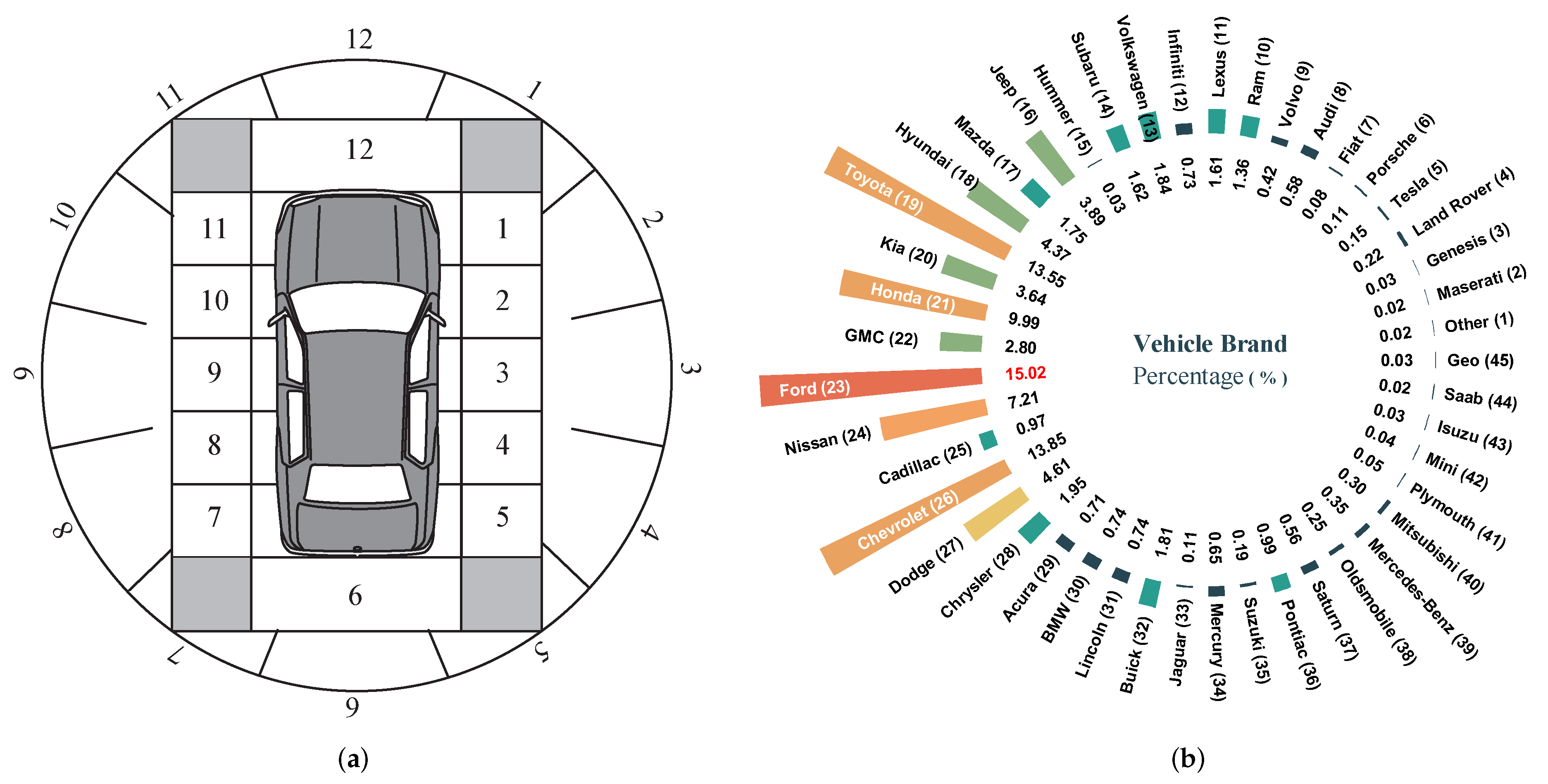
Figure 3.
Vehicle features in the accident dataset. (a) Diagram illustrating vehicle collision locations based on NHTSA classification [49]. (b) Distribution of vehicle brands (VEH_MKE) in the dataset. The number inside the circle represents the percentage of the corresponding brand in total accidents, while the number next to the brand name indicates its assigned label.
3. Data Description
This study uses crash data from the CRSS and FARS databases maintained by the NHTSA from 2016 to 2022. The CRSS provides a nationally representative sample of police-reported crashes, including those resulting in property damage, injuries, or fatalities, while the FARS records fatal crashes where at least one fatality occurs within 30 days of the accident. The two databases collectively include 594,773 crash cases, covering single-vehicle, two-vehicle, and multi-vehicle collisions, with PV-PV collisions being the most frequent, accounting for 225,461 cases. A detailed breakdown of the raw data is presented in Table 1. More information on these databases can be found at NHTSA CRSS and NHTSA FARS.
3.1. Descriptive Statistics of Accident Data
To ensure data completeness and reliability, accident cases missing critical feature information were removed. Since this study focuses on predicting the injury severity of the subject vehicle’s driver, certain attributes of the other party in the collision were considered less relevant. For instance, the seat belt usage of the other driver is unlikely to significantly impact the subject driver’s injury severity. Consequently, some cases were retained despite incomplete information on the other driver, resulting in instances where only one driver in a collision was analyzed.
After preprocessing, the final dataset comprises 116,998 accident cases and 182,296 drivers, ensuring that each retained case contains sufficient information for injury severity prediction. A detailed summary of the dataset after preprocessing is presented in Table 2, Table 3 and Table 4.
After applying the mRMR algorithm, the feature set was reduced from 65 to 33, achieving a balance between relevance and redundancy. At this selection point, feature redundancy is minimized, and further increasing the number of features does not yield noticeable improvements in predictive accuracy. The retained features encompass key accident-related factors, ensuring both robust model performance and meaningful interpretability in accident analysis. The correlation among the selected features, assessed using Cramér’s V [50], is visualized in 6. This refinement enhances model performance by ensuring the inclusion of only the most relevant and non-redundant features, which are categorized into three groups:
1) Environmental Features (7 features): These features are related to weather conditions and accident location. Table 2 presents all 7 environmental features.
2) Collision and Pre-Collision Features (8 features): These features describe the driver’s evasive actions before impact and the collision dynamics. Table 3 lists six of these features, while the initial impact areas of both vehicles (IMP_ARE1 and IMP_ARE2) are shown in Figure 4. For better visualization, the definition of the initial impact area of a vehicle is illustrated in Figure 3(a).
3) Participant Features (18 features): These features include driver and vehicle-related characteristics for both parties involved in the collision. Table 4 presents 14 of these features, the age distributions of the two drivers (DRV_AGE1 and DRV_AGE2) are illustrated in Figure 5, and the vehicle brand statistics of the involved vehicles are shown in Figure 3 (b).
This selection process ensures that the retained features contribute meaningfully to accident severity prediction while minimizing redundancy and noise in the dataset.
3.2. Feature Statistical Description
Building on the statistical analysis of environmental factors, accidents most frequently occur during daytime, under clear weather, on straight and level roads, and on two-way undivided roadways outside intersections—scenarios where vehicles spend most of their travel time. While crash frequency is high due to greater exposure, severe injuries are less common, as good visibility, well-maintained pavement, and predictable traffic flow enhance safety. However, two-way undivided roads stand out as an exception, exhibiting a relatively higher fatality risk despite their prevalence, likely due to the increased likelihood of high-speed head-on collisions.
Shifting focus to collision dynamics, pre-collision features play a crucial role in accident severity. Braking upon detecting danger is associated with a lower risk of fatal injuries (8%), whereas vehicle instability before impact—such as skidding laterally—correlates with a substantially higher severity risk (70.9%), likely due to factors such as slippery roads, excessive speed, and driver errors. Accident type (ACC_TYPE) also influences injury outcomes: rear-end collisions, though the most frequent, are linked to a relatively lower fatal injury risk (4.4%), while head-on collisions present the highest risk due to greater collision energy. Impact location further affects injury severity, with side impacts at the 9, 10, and 3 o’clock positions exhibiting significantly higher fatal injury risks (43.5%, 38.1%, and 35.3%, respectively), likely due to limited energy absorption and intrusion into the driver’s space.
It is important to note that since this study integrates two datasets with different class distributions—one covering all accident types and the other focusing on high-severity cases—the reported percentages indicate relative risk levels rather than absolute probabilities. Being struck by the front end (12 o’clock position) of the opposing vehicle poses the highest risk (28%). Similarly, higher pre-crash speeds (TRV_SPD1, TRV_SPD2) are strongly correlated with increased injury severity, while rollovers and loss-of-control crashes—often involving multiple impacts with objects such as the ground, trees, or guardrails—further elevate the risk of severe injuries.
An analysis of driver and vehicle characteristics identifies additional factors influencing injury severity. Male drivers exhibit a higher risk of fatal injury than female drivers, with Cramér’s V [50] analysis revealing significant associations between gender and vehicle attributes, including VEH_AGE1, VEH_BDY1, VEH_MKE1, and TRV_SPD. Furthermore, impairment due to alcohol consumption or drug influence is a critical factor associated with increased injury severity.
Finally, protective measures and vehicle attributes play a key role in reducing injury severity. Seat belt use and airbag deployment significantly lower injury severity, with non-deployed airbags typically seen in low-energy collisions that result in minor injuries. Heavier vehicles generally offer better protection due to lower collision accelerations, with vehicle weight also linked to structural attributes like height, width, and length that affect crash safety. Additionally, collisions involving minivans or cargo vans tend to result in less severe injuries, possibly due to factors such as professional drivers and lower urban speeds.
4. Experimental Results
To predict accident severity, five EML models and a Decision Tree model were employed, treating the prediction as a multi-class classification task. Model performance was evaluated using multiple metrics, as shown in Figure 6. Since accuracy alone does not provide a complete assessment, particularly in imbalanced classification problems, precision, recall, and F1-score were also used to ensure a more comprehensive evaluation.
Despite merging the CRSS and FARS databases, class imbalance persisted, with severity levels distributed as follows: Level 0 (45.3%), Level 1 (26.9%), Level 2 (8.8%), and Level 3 (19%). To mitigate this, random oversampling and undersampling techniques were applied, using the average class size as a benchmark. Classes exceeding the benchmark were downsampled, while those below it were upsampled. For synthetic data generation, categorical features remained unchanged, while numerical features were modified by adding random noise within ±10% of the original values to enhance data variability while preserving statistical integrity.
Bayesian optimization was employed to determine the optimal hyperparameters for each model, offering advantages such as reduced computational cost and efficient exploration of the hyperparameter space. Model performance was evaluated both before and after data balancing, with hyperparameters tuned separately for each scenario. The dataset was split into 60% training, 20% validation, and 20% testing sets.
Following data balancing, all models demonstrated significant performance improvements. As shown in Table 5, prior to balancing, XGBoost achieved the highest accuracy (79.52%) and precision (71.8%), while CatBoost excelled in recall (68.6%) and F1-score (68.69%). After balancing, XGBoost outperformed all models across all four metrics (Accuracy = 84.9%, Precision = 84.85%, Recall = 84.9%, F1-score = 84.87%), followed by Random Forest (Accuracy = 83.74%, Precision = 83.63%, Recall = 83.77%, F1-score = 83.66%). However, Decision Tree exhibited a slight accuracy decrease of 0.73% after balancing, despite notable improvements in precision, recall, and F1-score. This suggests that the model initially favored predicting the majority class in the imbalanced dataset. The redistribution of class instances reduced this bias, enhancing its ability to classify minority classes correctly, while causing a slight accuracy drop.
4.1. Accident Feature Analysis
Based on the model performance evaluation, XGBoost demonstrated superior performance across all metrics and was therefore selected as the target model for interpretability analysis in this study. The SHAP method, based on Shapley values (as detailed in Section 2), was employed to systematically interpret its decision-making mechanisms.
Global SHAP analysis quantitatively assessed the contributions of individual features to predictions across the four accident severity classes. Figure 7(a-d) illustrates the SHAP value distributions for different severity categories. The horizontal axis represents the range of SHAP values, indicating feature influence intensity (positive values support the prediction of the corresponding severity class, while negative values indicate opposing effects). The vertical axis lists feature variables, with scatter point colors representing feature magnitudes (for numerical variables) or encoded categorical labels (for nominal variables)
Analytical results indicate that TRV_SPD1 and TRV_SPD2 make the greatest contribution to Level 0 predictions, suggesting that the travel speeds of both collision parties play a crucial role in determining accident severity by influencing kinetic energy transfer. Lower velocities (cool-toned colors) increase the likelihood of Level 0 predictions, whereas higher velocities (warm-toned colors) lower the probability of being classified as Level 0.
Further investigation reveals that most features exhibit nonlinear relationships between their values and SHAP contributions. Most features exhibit a bimodal distribution, where lower-value ranges correspond to predominantly negative SHAP values, transitioning to positive values at higher ranges. Additionally, certain features display polarity reversal across different severity classes. This phenomenon suggests that the model captures context-dependent variations in feature contributions. Notably, vehicle speed parameters are strongly correlated with accident severity, supporting the validity of the model’s decision-making process and its consistency with fundamental collision dynamics principles.
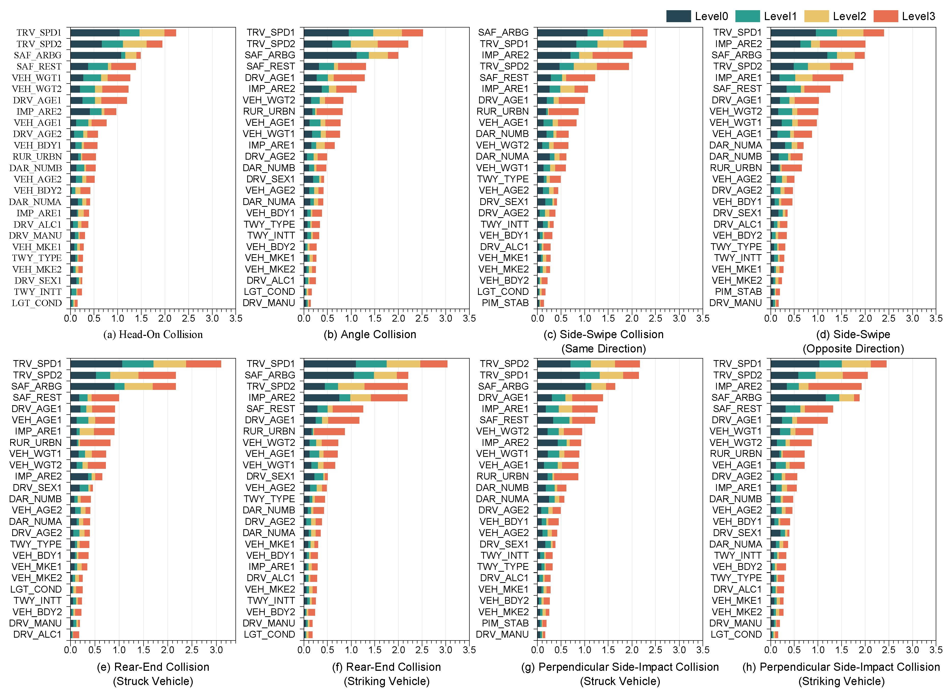
4.1.1. Feature Importance Analysis
Feature importance analysis is essential for understanding model decision-making and guiding accident analysis. While SHAP value distributions show how individual feature values impact predictions, they do not quantify the overall significance of features. To address this, the mean absolute SHAP value (Mean(|SHAP|)) is used to measure the average contribution of each feature across all predictions. The feature importance ranking results are shown in Figure 8, with the feature importance for another eight types of accidents presented in Figure A1. TRV_SPD1, TRV_SPD2, ACC_TYPE, and IMP_ARE2 are identified as the most influential features in the model. However, globally important features do not always align with those most critical for specific severity levels. For instance, the primary predictors for Level 3 severity are TRV_SPD2, DRV_AGE1, and SAF_ARBG.
Moreover, to assess the impact of feature importance on model performance, features were progressively removed in ascending order of importance, followed by model retraining and evaluation. The relationship between feature count and model accuracy, illustrated in Figure 9, demonstrates that retaining high-importance features results in significant performance improvements, while low-importance features contribute less substantially.
Although global rankings identify key predictors, they may overlook features with strong localized effects. For example, DRV_ALC1 ranks 22nd globally but exhibits widely dispersed SHAP values, indicating that despite its low frequency, it has a substantial impact on accident severity. This underscores the necessity of considering both overall and scenario-specific importance for a more comprehensive assessment of accident severity determinants.
4.1.2. Feature Dependency Analysis
In this study, feature dependency analysis is performed using the SHAP dependence plot, which captures the marginal effect of individual features on the target variable while illustrating the distribution and variability of SHAP values. Each point on the plot represents the predicted target value for a specific observation in the dataset. The analysis focuses on Level3 severity, representing fatal accidents—the most critical crash severity category. Thus, feature dependency analysis primarily examines feature behavior at this level to provide deeper insights into their contributions to fatal crash outcomes. Specifically, four key features—TRAV_SPD1, IMP_ARE1, VEH_MKE1, and VEH_BDY1—are analyzed. Additionally, the system autonomously identifies the feature with the strongest interaction within the dataset, as shown in Figure 10.
Figure 10(a) presents the interaction between TRV_SPD1 and DRV_SEX1. As TRV_SPD1 increases, the SHAP value shifts from negative to positive along the y-axis, with a transition threshold between 40 mph and 55 mph, indicating a critical speed range for predicting fatal accidents. The scatter point colors represent driver gender, revealing nearly identical SHAP distributions for male and female drivers. Although DRV_SEX1 exhibits a globally bimodal impact, its narrow SHAP distribution suggests a negligible overall influence compared to speed, whose broader distribution signifies a more substantial effect.
Figure 10(b) illustrates the interaction between IMP_ARE1 and IMP_ARE2, underscoring the strong association between impact location and fatal crash outcomes. Collisions at the 9 o’clock and 10 o’clock positions contribute most significantly to fatal injury predictions, aligning with real-world crash dynamics. These zones, located near the driver, absorb less impact energy, leading to severe structural deformation and reduced survival space. The effect is exacerbated when these areas are struck by another vehicle’s 11 o’clock or 12 o’clock positions, where impact forces are typically highest.
Figure 10(c) examines the influence of VEH_MKE1 and VEH_WGT1, demonstrating brand-specific variations in vehicle safety performance. The x-axis represents encoded vehicle brand labels (refer to Figure 4), allowing for a direct comparison of brand influence on accident severity. Scatter point colors denote vehicle curb weight, highlighting how certain manufacturers specialize in distinct vehicle categories. For example, Hummer (15) focuses on off-road vehicles, while RAM (10) primarily produces light trucks—both featuring high curb weights and reinforced body structures. Conversely, Volkswagen (13) and Tesla primarily manufacture passenger cars with lower curb weights but high safety ratings, aligning with their real-world safety reputations.
Figure 10(d) explores the relationship between VEH_BDY1 and VEH_WGT1, emphasizing the significant variation in crash survivability across vehicle body types. Light trucks exhibit lower susceptibility to fatal crashes compared to passenger vehicles (PVs), which are more prone to severe injuries. Scatter point colors indicate that light trucks generally have higher curb weights than PVs. Among body types, pickup trucks demonstrate the highest safety performance, whereas convertibles rank lowest, underscoring the critical role of vehicle structure and weight in crash outcomes.
4.1.3. Bivariate SHAP Contribution Analysis
Given that SHAP values exhibit additivity, the sum of individual feature SHAP values equals their cumulative contribution to the model’s prediction. This property allows for the evaluation of the combined impact of two or more features on the target variable by aggregating their SHAP values. In this study, Bivariate SHAP Contribution Analysis investigates the joint influence of feature pairs on model predictions by analyzing the sum of their SHAP values. This approach uncovers feature interactions and their collective impact on accident severity classification. By visualizing the aggregated SHAP contributions through a scatter heatmap, patterns emerge that show how specific feature combinations lead to higher or lower predicted severity levels, providing deeper insights into interdependent factors driving model decisions.
Figure 11 (a-d) displays the joint contribution of TRV_SPD1 & TRV_SPD2 to injury severity levels ("Level 0" to "Level 3"). The color of each scatter point reflects the magnitude of the SHAP value, illustrating how increasing vehicle speeds lead to higher predicted severity. Similarly, Figure 11 (e-h) depicts the combined effect of DRV_AGE1 & VEH_AGE1, showing that drivers over 80 years old are more likely to experience Level 3 injuries, with the age threshold decreasing as vehicle age increases, reflecting improvements in vehicle safety technologies. Figure 11 (i-l) demonstrates the joint influence of VEH_WGT1 & VEH_WGT2, revealing that heavier vehicles typically sustain lower injury severity compared to lighter vehicles in collisions.
This analysis effectively reveals the joint influence of feature pairs on accident severity outcomes. The clustering of colors within the heatmaps highlights distinct support, rejection, and transition regions. Red regions indicate the support domain, where predictions are more likely to align with the corresponding category, while deep blue regions represent the rejection domain, where predictions are less likely to belong to the specified category. Light green and light yellow regions correspond to transition zones, where predictions exhibit intermediate tendencies and neither strongly support nor reject the predicted outcomes. The clarity of these clusters underscores the contribution of these feature interactions in enhancing model prediction accuracy.
4.1.4. Instance-Level SHAP Interpretation
Instance-Level SHAP Interpretation decomposes the SHAP values for a single prediction instance, revealing the specific contribution of each feature to the final prediction and explaining why the model made that particular decision. Figure 12 presents the SHAP value waterfall plot for a randomly selected accident case from the dataset, where the actual injury severity is classified as "Level 3." The x-axis represents the SHAP values, while the y-axis lists the features in descending order of importance. The feature labeled ’Others’ represents the cumulative SHAP values of lower-contributing features, ensuring a more concise visualization.
The SHAP value waterfall plot provides an intuitive and transparent representation of the model’s decision-making process, illustrating how individual features contribute to the final prediction. The baseline value, , representing the expected model output across the dataset, is computed as 0.360, 0.568, 0.555, and 0.465 for injury severity levels 0 to 3, respectively. By aggregating the SHAP values of each feature relative to this baseline, the cumulative SHAP value for each severity level is obtained. The final predicted probabilities for each severity category are then derived using the Softmax function.
This instance-level interpretation enhances the explainability of the model by highlighting the key factors that influence the classification outcome. Such insights are particularly valuable for understanding the underlying risk factors in individual accident cases and can aid in data-driven decision-making for traffic safety analysis and policy development.
5. Implication and Limitations
5.1. Implications
This study focuses on driver injury severity prediction and factor analysis in PV-PV collisions, addressing a critical research gap in this domain. By leveraging interpretable machine learning techniques, we not only enhance prediction accuracy but also provide deeper insights into the key factors influencing injury severity, thereby informing traffic safety improvements and accident prevention strategies.
Moreover, by integrating the CRSS and FARS datasets, we have significantly mitigated the issue of class imbalance, reducing it by two orders of magnitude. This enhancement strengthens the model’s ability to predict high-severity injury cases, which are often underrepresented in imbalanced datasets. Given that accurately identifying severe injury cases is essential for emergency response planning and policy formulation, this improvement substantially increases the practical applicability of our findings.
Furthermore, this study employs SHAP to interpret the machine learning model, enabling a precise quantification of each feature’s impact, magnitude, and direction on injury severity. This interpretability not only enhances the model’s credibility but also provides actionable insights for stakeholders, such as policymakers and vehicle manufacturers, facilitating the development of targeted safety interventions.
5.2. Limitations
Despite the promising results, this study has certain limitations. Traffic accident analysis and injury severity prediction are inherently complex, and several critical factors cannot be accurately captured in structured datasets. For instance, driver psychological state and fatigue levels play a significant role in accident outcomes but are difficult to quantify. Additionally, the collision process itself is highly dynamic—secondary collisions triggered by the initial impact can significantly affect injury severity, yet these cascading effects are not well represented in traditional datasets. As a result, while our model provides valuable insights, its predictive capability remains limited by the absence of real-world complexity factors.
5.3. Future Work
Future research could enhance injury severity prediction by incorporating vision-based methods to automatically extract both macro-level (e.g., vehicle trajectories, collision impact forces) and micro-level (e.g., driver facial expressions, pre-crash behavior) features from accident videos. This approach would enable a more comprehensive understanding of the accident process, overcoming the limitations of relying solely on structured datasets that capture only a single moment in time. By integrating video-based accident reconstruction with machine learning, future studies could achieve a more dynamic and holistic analysis of crash events, which would lead to improved predictive performance and more effective safety interventions.
6. Conclusions
This study employed interpretable machine learning algorithms to predict driver injury severity and analyze accident characteristics in PV-PV collisions. The proposed prediction model achieved high accuracy, with superior precision, recall, and F1-score across all severity levels compared to existing studies. Notably, the model demonstrated significantly improved accuracy in predicting severe injury and fatality levels, which are the most critical categories in accident prediction and analysis. This improvement stems from the integration of the CRSS and FARS datasets, which mitigated class imbalance in high-severity cases, and the application of the mRMR algorithm, which reduced redundancy and refined feature selection.
By leveraging SHAP-based interpretable machine learning, this study provides a high-performance predictive model for injury analysis and accident causation studies in PV-PV collisions. Focusing on micro-level accident cases, the study identified the most influential features associated with accident occurrence and progression, ensuring a more precise and reliable prediction framework.
Global and local SHAP analyses revealed the contribution and directional impact of various accident-related features on injury severity prediction. Through multiple visualization techniques, the study examined both individual feature effects and combined feature interactions from different perspectives. These insights enhance the understanding of key accident factors, supporting more effective injury prevention strategies, risk assessment, and safety interventions. The proposed approach offers a robust framework for future research on accident severity prediction and interpretable machine learning applications in traffic safety analysis.
Author Contributions
Authors’ contributions can be summarized as follows: conceptualization, P.L., W.Y. and W.G.; methodology, P.L., W.Z., X.W., and W.G.; software, P.L., W.G. and W.Z.; validation, P.L. and X.W.; formal analysis, P.L. and W.Y.; resources, W.Y. and L.P.; investigation, P.L., W.Z. and X.W.; data curation, P.L. W.Y.; writing—original draft, P.L., W.Z. and W.G.; writing—review and editing, P.L., X.W., and W.Z.; visualization, P.L. and W.Y.; supervision, P.L., W.Z. and W.G. All authors have read and agreed to the published version of the manuscript.
Funding
This research received no external funding.
Institutional Review Board Statement
Not applicable.
Informed Consent Statement
Not applicable.
Data Availability Statement
The data presented in this study are derived from the publicly available NHTSA crash dataset, which can be accessed at https://www.nhtsa.gov/data/crash-data-systems. However, the processed dataset used in this study is available upon request from the corresponding author due to confidentiality and personal data protection regulations.
Acknowledgments
In this section you can acknowledge any support given which is not covered by the author contribution or funding sections. This may include administrative and technical support, or donations in kind (e.g., materials used for experiments).
Conflicts of Interest
Authors Jiejie Xu, Wangpengfei Yu and Yang Chen are em-ployed by the Shanghai Intelligent Vehicle cooperating Innovation Center. The remaining authors declare that the research was conducted in the absence of any commercial or financial relationships that could be construed as a potential conflict of interest.
Appendix A
Appendix A.1
Figure A1.
This is a figure. Schemes follow the same formatting.
References
- European Automobile Manufacturers’ Association (ACEA). ACEA Pocket Guide 2024 - 2025; Report No. N/A. European Automobile Manufacturers’ Association: Brussels, Belgium, 2024.
- International Transport Forum (ITF). Road Safety Annual Report 2024; OECD Publishing: Paris, France, 2024.
- Guo, W., Li, J., Song, X., & Zhang, W. (2025). A game-theoretic driver steering model with individual risk perception field generation. Accident Analysis & Prevention, 211, 107869. [CrossRef]
- International Organization for Standardization. ISO 3833:1977 - Road vehicles - Types - Terms and definitions. ISO, 1977.
- World Health Organization. Global status report on road safety 2023. Geneva: World Health Organization; 2023. Licence: CC BY-NC-SA 3.0 IGO.
- National Center for Statistics and Analysis. Traffic safety facts 2022: A compilation of motor vehicle traffic crash data; Report No. DOT HS 813 656. National Highway Traffic Safety Administration: Washington, DC, USA, 2024.
- Guo, W., Song, X., Zhang, W., Li, J., & Wu, X. (2024). Game-Theoretic Shared Control Strategy for Cooperative Collision Avoidance Under Extreme Conditions. IEEE Transactions on Vehicular Technology. [CrossRef]
- Chand, Arun, Jayesh, S., and Bhasi, A. B. Road traffic accidents: An overview of data sources, analysis techniques and contributing factors. Materials Today: Proceedings, vol. 47, pp. 5135–5141, 2021. [CrossRef]
- Pourroostaei Ardakani, S., Liang, X., Mengistu, K. T., So, R. S., Wei, X., He, B., & Cheshmehzangi, A. (2023). Road car accident prediction using a machine-learning-enabled data analysis. Sustainability, 15(7), 5939. [CrossRef]
- Setiadi, D. R. I. M., Islam, H. M. M., Trisnapradika, G. A., & Herowati, W. (2024). Analyzing preprocessing impact on machine learning classifiers for cryotherapy and immunotherapy dataset. Journal of Future Artificial Intelligence and Technologies, 1(1), 39–50.
- Otchere, D. A., Ganat, T. O. A., Ojero, J. O., Tackie-Otoo, B. N., & Taki, M. Y. (2022). Application of gradient boosting regression model for the evaluation of feature selection techniques in improving reservoir characterisation predictions. Journal of Petroleum Science and Engineering, 208, 109244 . [CrossRef]
- Song, D., Yang, X., Yang, Y., Cui, P., and Zhu, G. Bivariate joint analysis of injury severity of drivers in truck-car crashes accommodating multilayer unobserved heterogeneity. Accident Analysis & Prevention, vol. 190, p. 107175, 2023. [CrossRef]
- Gong, H., Fu, T., Sun, Y., Guo, Z., Cong, L., Hu, W., and Ling, Z. Two-vehicle driver-injury severity: A multivariate random parameters logit approach. Analytic Methods in Accident Research, vol. 33, p. 100190, 2022. [CrossRef]
- Kim, J.-K., Ulfarsson, G. F., Kim, S., and Shankar, V. N. Driver-injury severity in single-vehicle crashes in California: a mixed logit analysis of heterogeneity due to age and gender. Accident Analysis & Prevention, vol. 50, pp. 1073–1081, 2013. [CrossRef]
- Cerwick, D. M., Gkritza, K., Shaheed, M. S., and Hans, Z. A comparison of the mixed logit and latent class methods for crash severity analysis. Analytic Methods in Accident Research, vol. 3, pp. 11–27, 2014. [CrossRef]
- Santos, K., Dias, J. P., and Amado, C. A literature review of machine learning algorithms for crash injury severity prediction. Journal of Safety Research, vol. 80, pp. 254–269, 2022. [CrossRef]
- Ching-Hsue Cheng, Jun-He Yang, and Po-Chien Liu, "Rule-based classifier based on accident frequency and three-stage dimensionality reduction for exploring the factors of road accident injuries," PLoS One, vol. 17, no. 8, pp. e0272956, 2022. Public Library of Science San Francisco, CA USA. [CrossRef]
- Fazle Subhan, Yasir Ali, and Shengchuan Zhao, "Unraveling preference heterogeneity in willingness-to-pay for enhanced road safety: A hybrid approach of machine learning and quantile regression," Accident Analysis & Prevention, vol. 190, p. 107176, 2023. [CrossRef]
- J. Li, J. Liu, P. Liu, and Y. Qi, "Analysis of Factors Contributing to the Severity of Large Truck Crashes," Entropy, vol. 22, no. 11, p. 1191, Oct. 2020. [CrossRef]
- G. Shiran, R. Imaninasab, and R. Khayamim, "Crash Severity Analysis of Highways Based on Multinomial Logistic Regression Model, Decision Tree Techniques, and Artificial Neural Network: A Modeling Comparison," Sustainability, vol. 13, no. 10, p. 5670, May 2021. [CrossRef]
- Y. Liang, H. Yuan, Z. Wang, Z. Wan, T. Liu, B. Wu, S. Chen, and X. Tang, "Nonlinear effects of traffic statuses and road geometries on highway traffic accident severity: A machine learning approach," PLoS One, vol. 19, no. 11, p. e0314133, 2024. Public Library of Science San Francisco, CA USA. [CrossRef]
- Jamal, A., Zahid, M., Tauhidur Rahman, M., Al-Ahmadi, H. M., Almoshaogeh, M., Farooq, D., & Ahmad, M. (2021). Injury severity prediction of traffic crashes with ensemble machine learning techniques: A comparative study. International Journal of Injury Control and Safety Promotion, 28(4), 408–427. [CrossRef]
- Shaik, M. E., Islam, M. M., & Hossain, Q. S. (2021). A review on neural network techniques for the prediction of road traffic accident severity. Asian Transport Studies, 7, 100040. [CrossRef]
- Yu, L., Du, B., Hu, X., Sun, L., Han, L., & Lv, W. (2021). Deep spatio-temporal graph convolutional network for traffic accident prediction. Neurocomputing, 423, 135–147. [CrossRef]
- Alhaek, F., Liang, W., Rajeh, T. M., Javed, M. H., & Li, T. (2024). Learning spatial patterns and temporal dependencies for traffic accident severity prediction: A deep learning approach. Knowledge-Based Systems, 286, 111406. [CrossRef]
- Yan, M., & Shen, Y. (2022). Traffic accident severity prediction based on random forest. Sustainability, 14(3), 1729. [CrossRef]
- Wu, S., Yuan, Q., Yan, Z., & Xu, Q. (2021). Analyzing accident injury severity via an extreme gradient boosting (XGBoost) model. Journal of Advanced Transportation, 2021(1), 3771640. [CrossRef]
- Guo, M., Yuan, Z., Janson, B., Peng, Y., Yang, Y., & Wang, W. (2021). Older pedestrian traffic crashes severity analysis based on an emerging machine learning XGBoost. Sustainability, 13(2), 926. [CrossRef]
- Dong, S., Khattak, A., Ullah, I., Zhou, J., & Hussain, A. (2022). Predicting and analyzing road traffic injury severity using boosting-based ensemble learning models with SHAPley Additive exPlanations. International Journal of Environmental Research and Public Health, 19(5), 2925. [CrossRef]
- Zahid, M., Habib, M. F., Ijaz, M., Ameer, I., Ullah, I., Ahmed, T., & He, Z. (2024). Factors affecting injury severity in motorcycle crashes: Different age groups analysis using CatBoost and SHAP techniques. Traffic Injury Prevention, 25(3), 472–481. [CrossRef]
- Ahmed, S., Hossain, M. A., Bhuiyan, M. M. I., & Ray, S. K. (2021). A comparative study of machine learning algorithms to predict road accident severity. In 2021 20th International Conference on Ubiquitous Computing and Communications (IUCC/CIT/DSCI/SmartCNS) (pp. 390–397).
- Wen, X., Xie, Y., Jiang, L., Li, Y., & Ge, T. (2022). On the interpretability of machine learning methods in crash frequency modeling and crash modification factor development. Accident Analysis & Prevention, 168, 106617. [CrossRef]
- Lundberg, S. M., Erion, G., Chen, H., et al. (2020). From local explanations to global understanding with explainable AI for trees. Nature Machine Intelligence, 2, 56–67. [CrossRef]
- Ahmed, S., Hossain, M. A., Ray, S. K., Bhuiyan, M. M. I., & Sabuj, S. R. (2023). A study on road accident prediction and contributing factors using explainable machine learning models: Analysis and performance. Transportation Research Interdisciplinary Perspectives, 19, 100814. [CrossRef]
- Boo, Y., & Choi, Y. (2022). Comparison of mortality prediction models for road traffic accidents: an ensemble technique for imbalanced data. BMC Public Health, 22(1), 1476. [CrossRef]
- Wongvorachan, T., He, S., & Bulut, O. (2023). A comparison of undersampling, oversampling, and SMOTE methods for dealing with imbalanced classification in educational data mining. Information, 14(1), 54. [CrossRef]
- Peng, H., Long, F., & Ding, C. (2005). Feature selection based on mutual information criteria of max-dependency, max-relevance, and min-redundancy. IEEE Transactions on Pattern Analysis and Machine Intelligence, 27(8), 1226–1238. [CrossRef]
- Toğaçar, M., Ergen, B., Çömert, Z., & Özyurt, F. (2020). A deep feature learning model for pneumonia detection applying a combination of mRMR feature selection and machine learning models. IRBM, 41(4), 212–222. [CrossRef]
- HK, R., HA, D., MS, P. K., S, S., & GH, Y. (2024). A robust framework for Alzheimer’s disease detection and staging: incorporating multi-feature integration, MRMR feature selection, and Random Forest classification. Multimedia Tools and Applications, 1–29. [CrossRef]
- Wang, G., Lauri, F., & Hassani, A. H. E. (2022). Feature selection by mRMR method for heart disease diagnosis. IEEE Access, 10, 100786-100796. [CrossRef]
- S. Rezvani and X. Wang, A broad review on class imbalance learning techniques, Applied Soft Computing, vol. 143, p. 110415, 2023. [CrossRef]
- Kingsford, C., and Salzberg, S. L. What are decision trees? Nature Biotechnology, vol. 26, no. 9, pp. 1011–1013, 2008. Nature Publishing Group US New York.
- L. Breiman, "Random forests," Machine Learning, vol. 45, pp. 5–32, 2001. [CrossRef]
- G. Ke, Q. Meng, T. Finley, T. Wang, W. Chen, W. Ma, Q. Ye, and T.-Y. Liu, "LightGBM: A highly efficient gradient boosting decision tree," Advances in Neural Information Processing Systems, vol. 30, 2017.
- T. Chen and C. Guestrin, "XGBoost: A scalable tree boosting system," in Proceedings of the 22nd ACM SIGKDD International Conference on Knowledge Discovery and Data Mining, pp. 785–794, 2016.
- L. Prokhorenkova, G. Gusev, A. Vorobev, A. V. Dorogush, and A. Gulin, "CatBoost: Unbiased boosting with categorical features," Advances in Neural Information Processing Systems, vol. 31, 2018.
- Y. Freund and R. E. Schapire, "A decision-theoretic generalization of on-line learning and an application to boosting," Journal of Computer and System Sciences, vol. 55, no. 1, pp. 119–139, 1997. [CrossRef]
- S. M. Lundberg, G. Erion, H. Chen, et al., "From local explanations to global understanding with explainable AI for trees," Nature Machine Intelligence, vol. 2, pp. 56–67, 2020. [CrossRef]
- National Center for Statistics and Analysis. (2024, April). Fatality Analysis Reporting System analytical user’s manual, 1975-2022 (Report No. DOT HS 813 556). National Highway Traffic Safety Administration.
- A. Agresti, Categorical Data Analysis, John Wiley & Sons, 2013.
Figure 1.
Schematic diagram of a traffic accident scene. The accident occurred as a sedan was overtaking a cargo van on the left. A pedestrian suddenly entered the lane, and due to the obstruction from the roadside greenery, the sedan driver did not notice the pedestrian in time. After noticing the pedestrian, the driver immediately braked and swerved left, causing a rear-end collision with the cargo van.
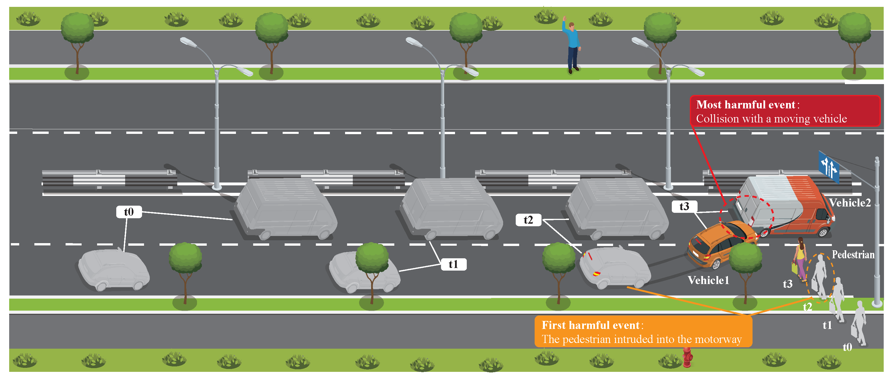
Figure 2.
Technical framework diagram of this study.
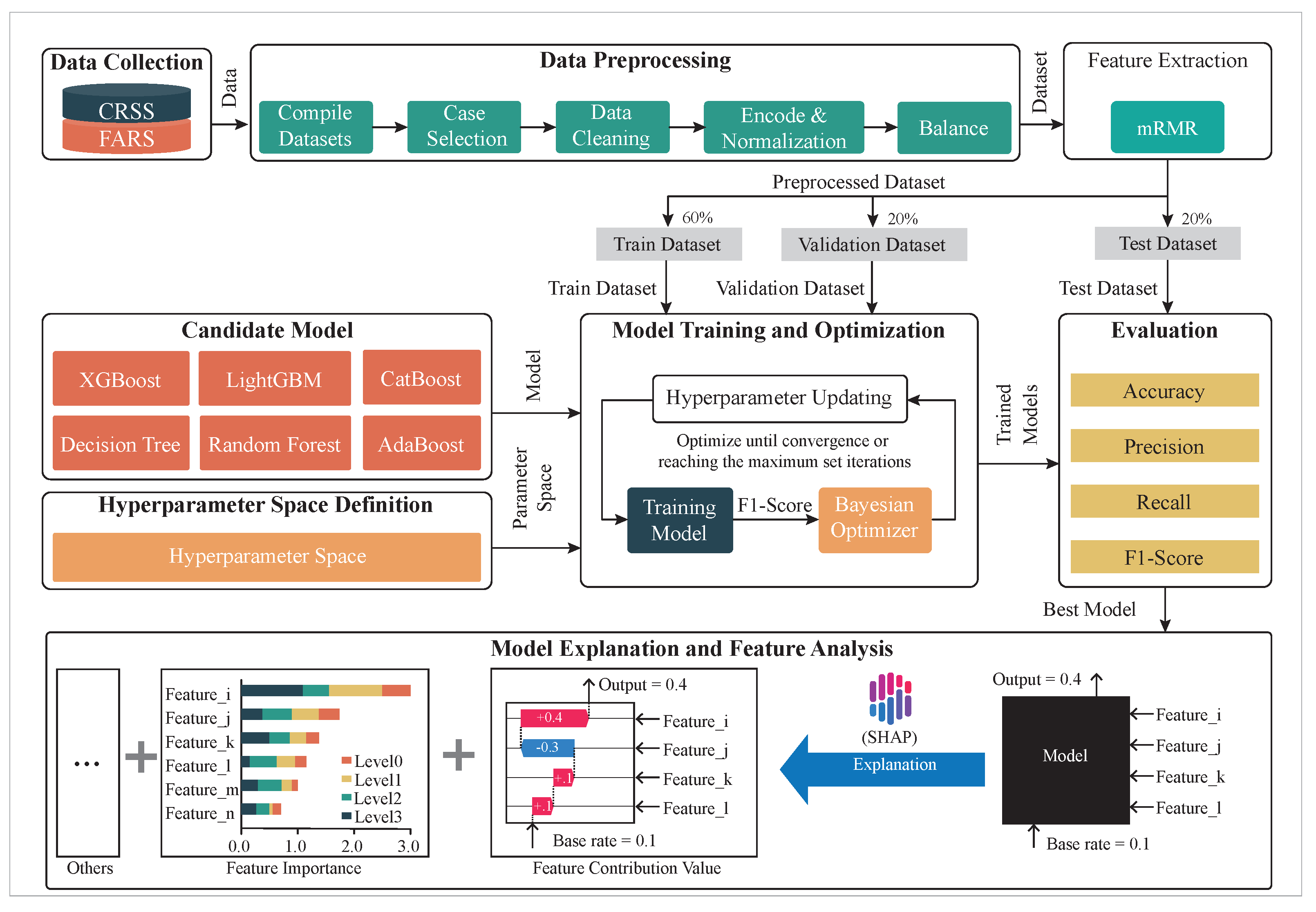
Figure 4.
Stacked chart of collision characteristics and severity. (a) Annual distribution. (b) Initial impact area of this vehicle (IMP_ARE1). (c) Driver age of this vehicle (DRV_AGE1). (d) Days of the week. (e) Initial impact area of the other vehicle (IMP_ARE2). (f) Driver age of the other vehicle (DRV_AGE2).
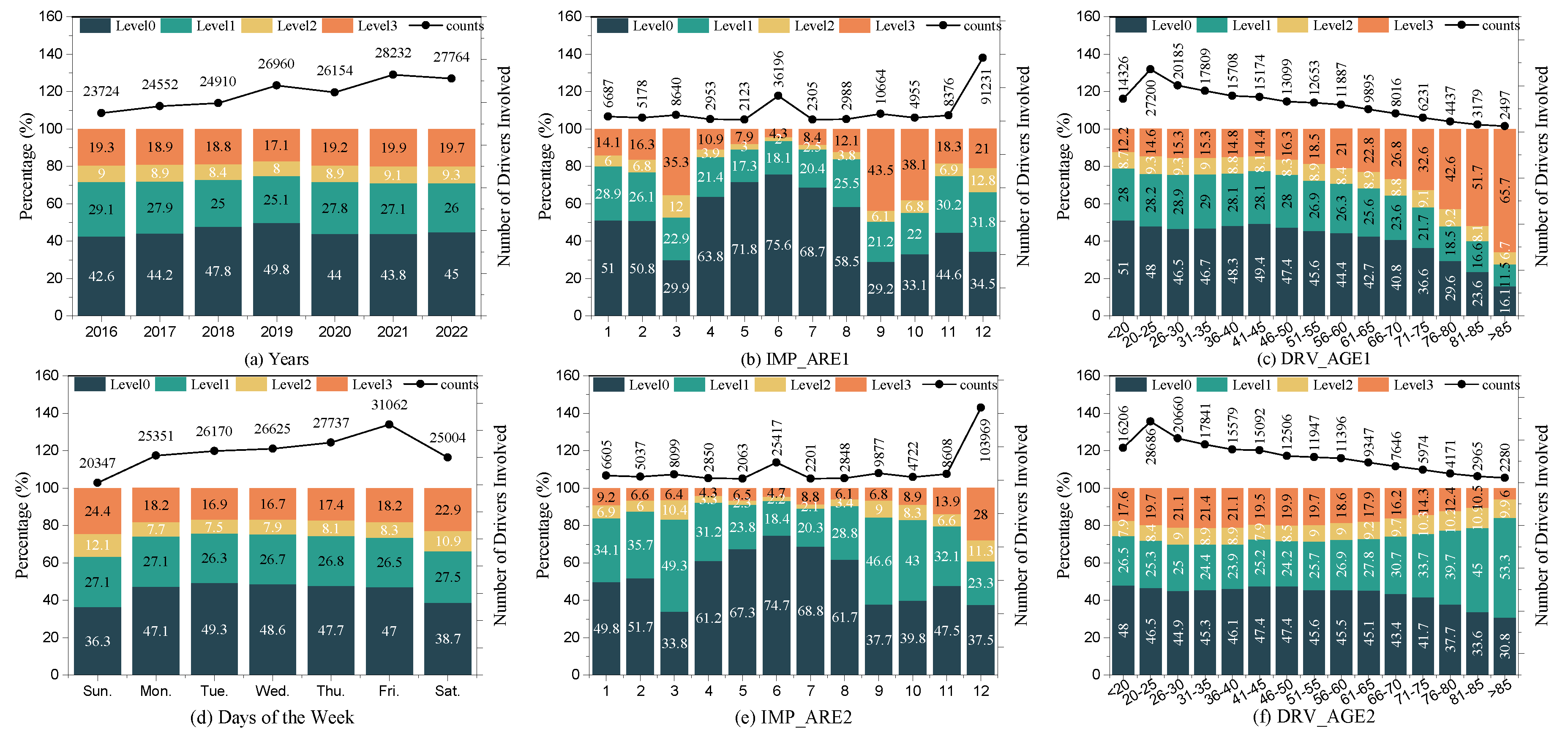
Figure 5.
Cramér’s V correlation matrix of selected accident features.
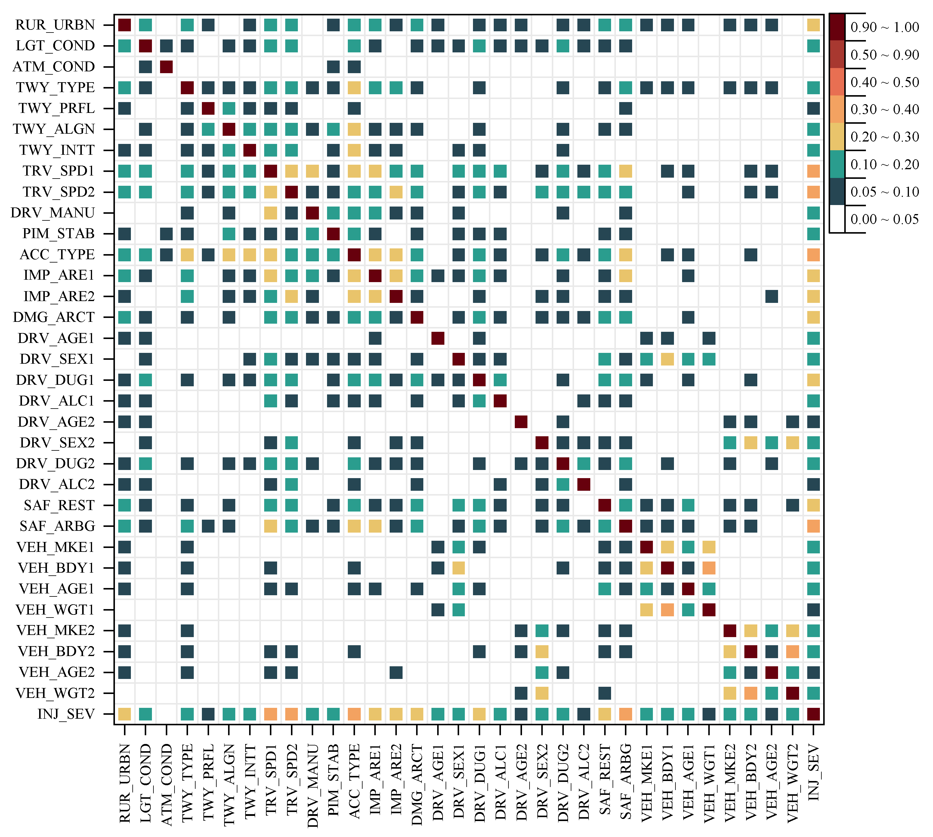
Figure 6.
Performance Metrics for Multiclass Classification Models.
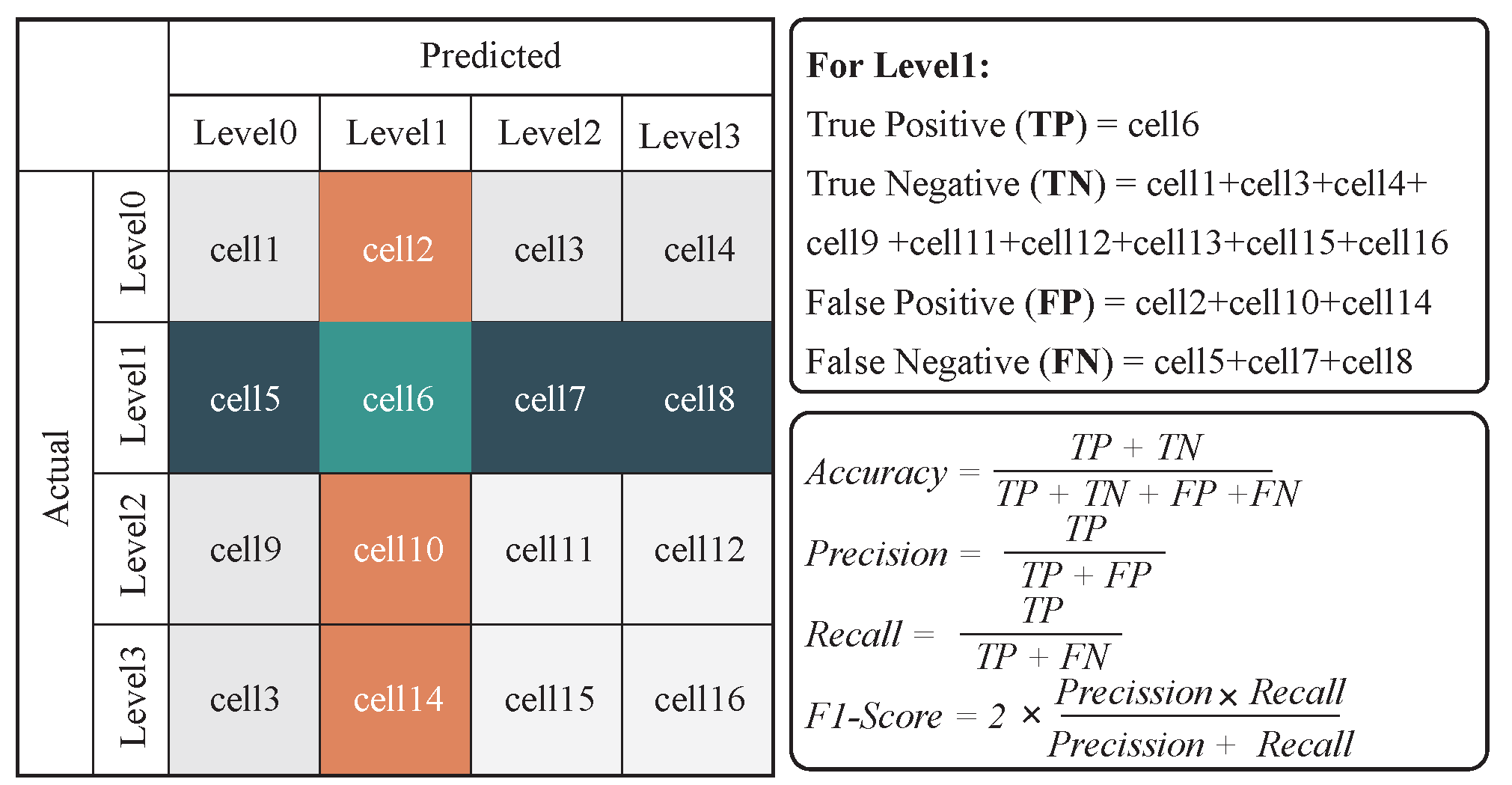
Figure 7.
Global SHAP value distribution of accident features.
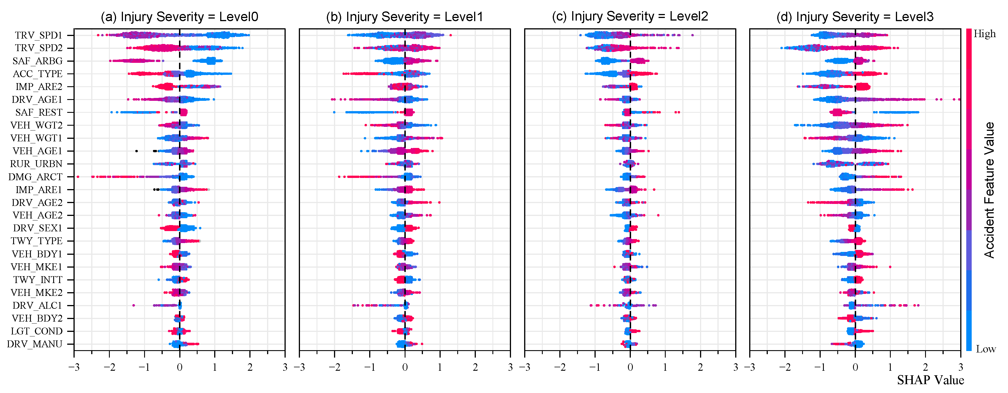
Figure 8.
Global feature importance ranking.
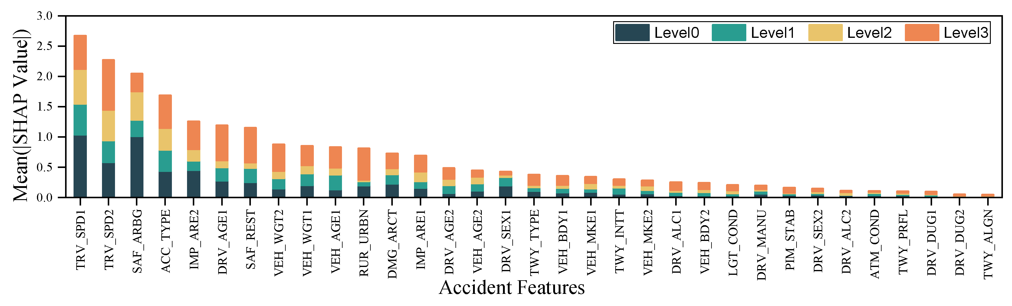
Figure 9.
Relationship between feature numbers and model performance.
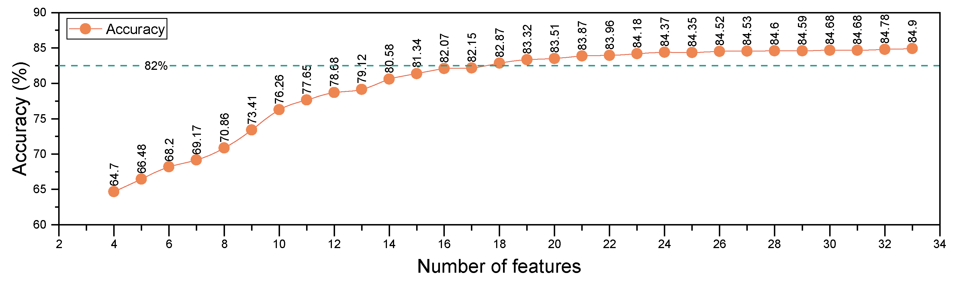
Figure 10.
Global SHAP value distribution of accident features.
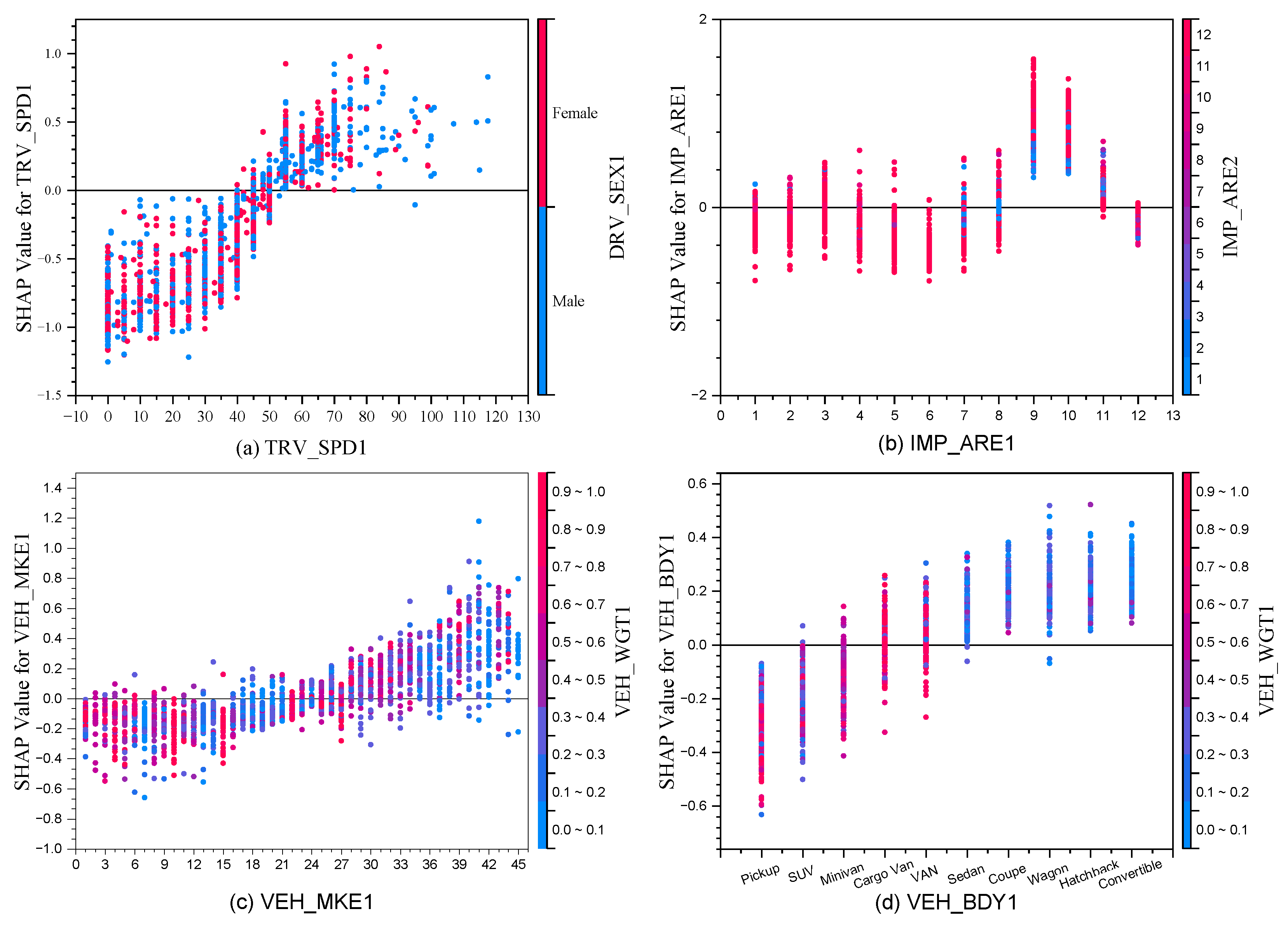
Figure 11.
Scatter plot of combined SHAP impact on accident severity. (a–d) TRV_SPD1 and TRV_SPD2, (e–h) DRV_AGE1 and VEH_AGE1, and (i–l) VEH_WGT1 and VEH_WGT2, with all plots showing combined SHAP values for injury severity levels (Level 0–Level 3).
Figure 11.
Scatter plot of combined SHAP impact on accident severity. (a–d) TRV_SPD1 and TRV_SPD2, (e–h) DRV_AGE1 and VEH_AGE1, and (i–l) VEH_WGT1 and VEH_WGT2, with all plots showing combined SHAP values for injury severity levels (Level 0–Level 3).
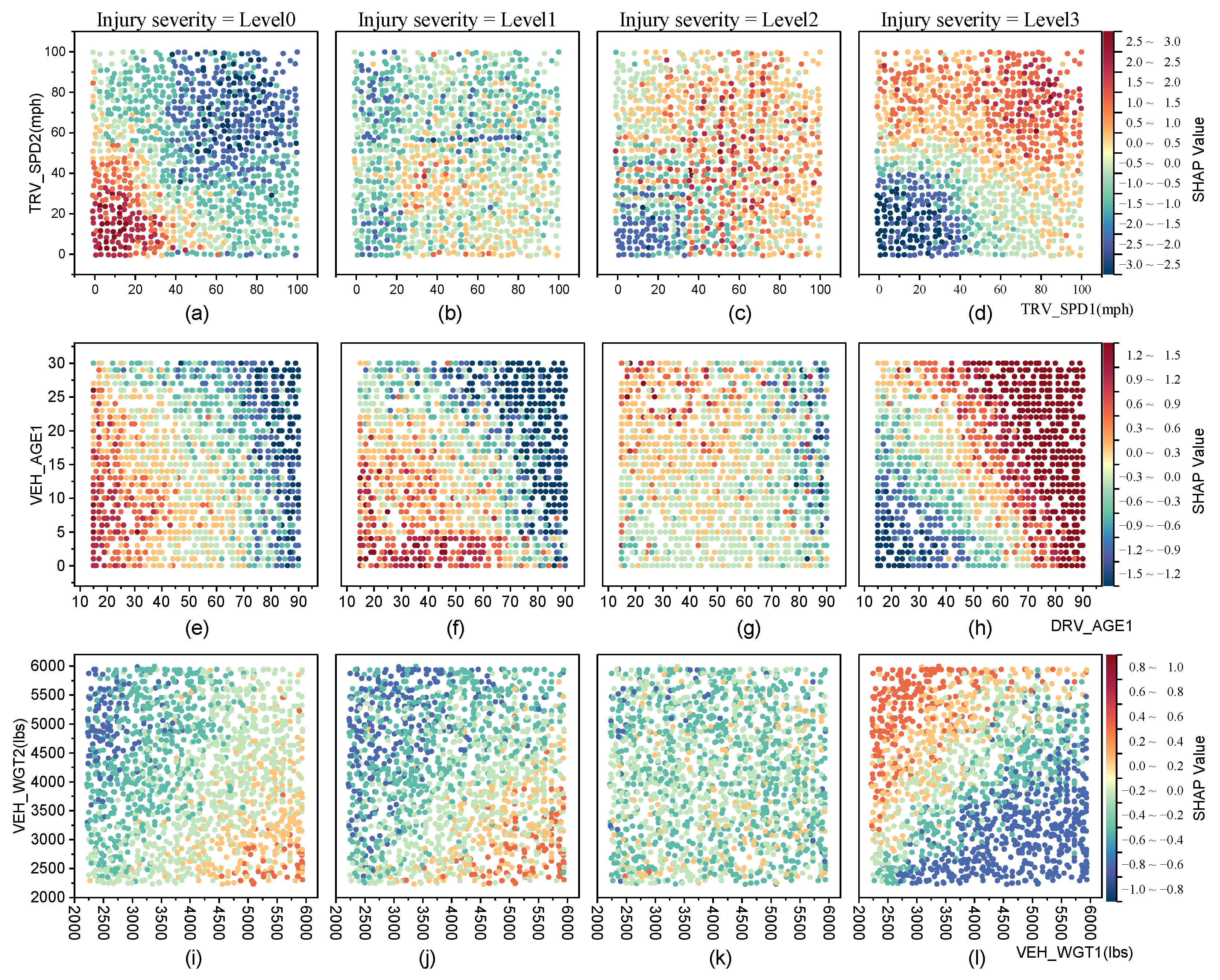
Figure 12.
Local SHAP waterfall plot for a single multi-class prediction case (True label: ’Level 3’).
Figure 12.
Local SHAP waterfall plot for a single multi-class prediction case (True label: ’Level 3’).
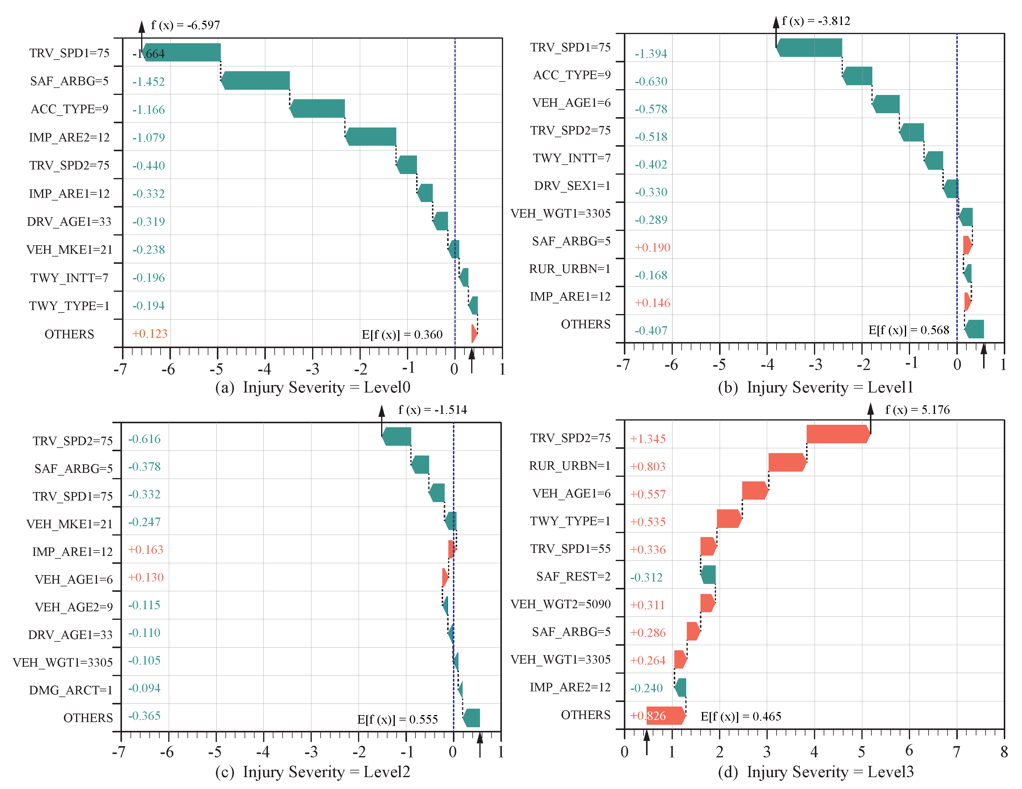

Table 1.
Accident data statistics from the CRSS and FARS databases (2016–2022).
| Database | Participants | Case Number | Driver numbers for different accident vehicles | |||||||
|---|---|---|---|---|---|---|---|---|---|---|
| Total | PV-PV | Total | PV | Motorcycle | Truck | Bus | Others | |||
| CRSS | 1 | 121288 | - | 121288 | 107169 | 8585 | 3768 | 418 | 1348 | |
| 2 | 204916 | 175910 | 409832 | 379053 | 9341 | 14218 | 1590 | 5630 | ||
| >2 | 26938 | - | 87755 | 83664 | 883 | 2226 | 122 | 860 | ||
| FARS | 1 | 134982 | - | 134982 | 111851 | 14360 | 5462 | 370 | 2939 | |
| 2 | 86718 | 49551 | 173436 | 132888 | 18678 | 17512 | 580 | 3778 | ||
| >2 | 19931 | - | 69080 | 57565 | 3685 | 6361 | 177 | 1292 | ||
| CRSS+FARS | - | 594773 | 225461 | 996373 | 872190 | 55532 | 49547 | 3257 | 15847 | |
Data source: National Highway Traffic Safety Administration (NHTSA), Crash Data Systems. Available at: https://www.nhtsa.gov/data/crash-data-systems.
Table 2.
Statistical description of accident environmental characteristics.
| Variables | (%) | Injury Severity (%) | Variables | (%) | Injury Severity (%) | ||||||
|---|---|---|---|---|---|---|---|---|---|---|---|
| 0 | 1 | 2 | 3 | 0 | 1 | 2 | 3 | ||||
| Database | Divided, Unprotected (2) | 27.7 | 50.2 | 31.2 | 6.6 | 12 | |||||
| CRSS | 63.3 | 68.7 | 27.7 | 3.2 | 0.4 | Divided, Protected (3) | 13.4 | 58 | 22.8 | 5.6 | 13.6 |
| FARS | 36.7 | 5 | 25.5 | 18.4 | 51.1 | One-Way (4) | 7.4 | 72.5 | 19.9 | 3.1 | 4.6 |
| CRSS+FARS | 100 | 45.3 | 26.9 | 8.8 | 19 | Roadway Profile (TWY_PRFL) | |||||
| Location at rural or urban (RUR_URBN) | Level (1) | 85.9 | 47.5 | 26.9 | 8.1 | 17.5 | |||||
| Rural (1) | 67.9 | 53 | 25.6 | 7.7 | 13.7 | Grade (2) | 7.2 | 36.1 | 27.7 | 11.4 | 24.8 |
| Urban (2) | 32.1 | 29.1 | 29.5 | 11.3 | 30.2 | Uphill (3) | 2.4 | 28.8 | 25.7 | 15 | 30.5 |
| Light condition (LGT_COND) | Downhill (4) | 2.7 | 31.2 | 24.5 | 13.6 | 30.7 | |||||
| Daylight (1) | 69.8 | 50.6 | 26.8 | 7.2 | 15.4 | Hillcrest (5) | 1.5 | 23.2 | 27.3 | 15.2 | 34.3 |
| Dawn (2) | 1.6 | 34 | 25 | 12 | 29.1 | Sag (6) | 0.2 | 26.6 | 31.2 | 11.6 | 30.7 |
| Dusk (3) | 2.6 | 47.6 | 24.8 | 9.3 | 18.3 | Roadway Alignment (TWY_ALGN) | |||||
| Dark-Lighted (4) | 15 | 41.1 | 30.5 | 9.4 | 19 | Straight (1) | 91.6 | 47.2 | 27.4 | 8.1 | 17.4 |
| Dark-Not Lighted (5) | 11 | 19.2 | 22.9 | 17.5 | 40.4 | Curve Right (2) | 4.6 | 31.1 | 19.1 | 14.9 | 35 |
| Atmospheric Conditions (ATM_COND) | Curve Left (3) | 3.8 | 18 | 24 | 19.5 | 38.5 | |||||
| Clear (1) | 74.4 | 46.3 | 26.6 | 8.6 | 18.5 | Type of Intersection (TWY_INTT) | |||||
| Cloudy (2) | 14.8 | 43.1 | 27.6 | 9.3 | 20.1 | Four-Way Intersection (1) | 33.7 | 45.9 | 33.3 | 6.8 | 14 |
| Rain (3) | 8.6 | 44.5 | 27.6 | 8.6 | 19.2 | T-Intersection (2) | 14.4 | 46.2 | 34.1 | 6.2 | 13.5 |
| Snow (4) | 1.2 | 41.3 | 26.8 | 11.1 | 20.9 | Roundabout (3) | 0.2 | 84.4 | 13.4 | 0.6 | 1.6 |
| Fog (5) | 0.6 | 17.7 | 24.6 | 17.6 | 40.1 | Five-Point, or more (4) | 0.2 | 55.5 | 29.7 | 5.9 | 8.9 |
| Other (6) | 0.3 | 22 | 26.4 | 17.3 | 34.4 | Y-Intersection (5) | 0 | 47.2 | 33.3 | 2.8 | 16.7 |
| Trafficway Description (TWY_TYPE) | Other Type (6) | 0.4 | 29.8 | 29.8 | 11.3 | 29.1 | |||||
| Not Divided (1) | 51.5 | 35.6 | 26.6 | 11.6 | 26.2 | Not an Intersection (7) | 51.1 | 44.7 | 20.6 | 10.9 | 23.9 |
Table 3.
Statistical description of collision and pre-collision characteristics.
| Variables | (%) | Injury Severity (%) | Variables | (%) | Injury Severity (%) | ||||||
|---|---|---|---|---|---|---|---|---|---|---|---|
| 0 | 1 | 2 | 3 | 0 | 1 | 2 | 3 | ||||
| Attempted Avoidance Maneuver (DRV_MANU) | Intersect Paths ( Straight Path) (7) | 14.3 | 26.1 | 40.6 | 9.9 | 23.5 | |||||
| No Avoidance Maneuver (1) | 23.7 | 62.6 | 17.6 | 5.7 | 14.2 | Opposite Direction (Angle Sideswipe) (8) | 4.2 | 12.4 | 28.4 | 16.5 | 42.8 |
| Braking (2) | 3.5 | 51.6 | 32.8 | 7.5 | 8.2 | Head-On (9) | 14.7 | 2.2 | 16.1 | 27.1 | 54.6 |
| Unknown (3) | 68 | 40.7 | 29.5 | 9.3 | 20.5 | Other Types (10) | 0.3 | 8.2 | 23.4 | 10.9 | 57.5 |
| Accelerating (4) | 0.1 | 39.5 | 29.3 | 10.9 | 20.4 | Travel Speed of This Vehicle (TRV_SPD1) | |||||
| Braking and Steering (5) | 1 | 24.7 | 35.9 | 18.3 | 21 | 0 mph | 16.2 | 84.6 | 11.3 | 1.4 | 2.7 |
| Releasing Brakes (6) | 0 | 22.9 | 41.7 | 2.1 | 33.3 | 0-20 mph | 19 | 82.2 | 8.8 | 2.2 | 6.8 |
| Braking and Unknown Steering Direction (7) | 0.2 | 13.4 | 42.9 | 18.8 | 25 | 21-40 mph | 27.1 | 38.1 | 41.5 | 7.2 | 13.2 |
| Steering (8) | 3.5 | 20.9 | 28.6 | 19 | 31.5 | 41-60 mph | 28.2 | 15.5 | 34.2 | 16.2 | 34.1 |
| Accelerating and Steering (9) | 0 | 26.1 | 19.5 | 16.3 | 38.2 | >60 mph | 9.4 | 13.7 | 25.9 | 17.4 | 43.1 |
| Pre-Impact Stability (PIM_STAB) | Travel Speed of Other Vehicle (TRV_SPD2) | ||||||||||
| Tracking (1) | 92.6 | 48 | 27.1 | 8.2 | 16.7 | 0 mph | 10 | 73 | 21.2 | 2.4 | 3.4 |
| Skidding Longitudinally (2) | 1.4 | 26.5 | 31.1 | 14.5 | 27.9 | 0-20 mph | 18.9 | 79.3 | 15.9 | 2.4 | 2.3 |
| Skidding Laterally (3) | 1.1 | 5.6 | 8.5 | 14.9 | 70.9 | 21-40 mph | 30 | 46.8 | 35.8 | 6.4 | 11 |
| Other (4) | 4.9 | 10.2 | 24.9 | 17.2 | 47.7 | 41-60 mph | 30.9 | 23.1 | 28.4 | 14.7 | 33.8 |
| Crash Type (ACC_TYPE) | >60 mph | 10.1 | 18.2 | 21.4 | 16.2 | 44.2 | |||||
| Rear End (1) | 32.1 | 74.9 | 18.6 | 2.1 | 4.4 | Damage Area Count (DMG_ARCT) | |||||
| Same Direction (Angle,Sideswipe) (2) | 7 | 79 | 11 | 1.8 | 8.2 | 1 | 55.9 | 52.9 | 26.1 | 6.9 | 14 |
| Miss Control (3) | 1.2 | 90.1 | 6.5 | 1.1 | 2.4 | 2-5 | 35.2 | 44.1 | 30.9 | 8.4 | 16.6 |
| Turn Into Path (4) | 12.2 | 42.1 | 37.2 | 5.9 | 14.8 | 6-9 | 4.7 | 4.7 | 20.1 | 22.2 | 53 |
| Turn Across Path (5) | 13.5 | 36 | 43.8 | 7.9 | 12.2 | 10-12 | 4.2 | 1.1 | 10.4 | 21.9 | 66.6 |
| Opposite direction (Forward Impact) (6) | 0.4 | 1.7 | 34.7 | 21.9 | 41.7 | ||||||
Table 4.
Statistical description of vehicle and driver characteristics for both parties in the collision.
Table 4.
Statistical description of vehicle and driver characteristics for both parties in the collision.
| Variables | (%) | Injury Severity (%) | Variables | (%) | Injury Severity (%) | ||||||
|---|---|---|---|---|---|---|---|---|---|---|---|
| 0 | 1 | 2 | 3 | 0 | 1 | 2 | 3 | ||||
| The gender of this driver (DRV_SEX1) | <1 | 4.7 | 54.8 | 21.5 | 6.5 | 17.2 | |||||
| Male (1) | 55.9 | 44.7 | 23.7 | 9.5 | 22 | 1-10 | 55.9 | 49.3 | 24.7 | 7.6 | 18.4 |
| Female (2) | 44.1 | 46.2 | 30.8 | 7.9 | 15.2 | 11-20 | 34.1 | 39.6 | 29.8 | 10.5 | 20.1 |
| Drug involvement of this driver (DRV_DUG1) | >20 | 5.3 | 32.4 | 35.3 | 12.7 | 19.7 | |||||
| No (1) | 96.6 | 46.8 | 27.2 | 8.3 | 17.7 | The Weight of This Vehicle (VEH_WGT1) | |||||
| Yes (2) | 3.4 | 3.9 | 17.1 | 22.5 | 56.6 | 1700-2700 lbs. | 8.5 | 38.2 | 21.3 | 8.2 | 32.5 |
| Alcohol Test Result of this driver (DRV_ALC1) | 2701-3700 lbs. | 51.9 | 44.8 | 25.9 | 8.4 | 21 | |||||
| 0 mg/dL | 93.7 | 48 | 27.4 | 8.2 | 16.5 | 3701-4700 lbs. | 26.3 | 48.3 | 28.3 | 9.2 | 14.2 |
| 1-80 mg/dL | 1 | 2.7 | 14.8 | 15.9 | 66.5 | 4701-5700 lbs. | 11.2 | 47.4 | 30.6 | 10.1 | 11.9 |
| >80 mg/dL | 5.4 | 7.7 | 18.7 | 19 | 54.6 | >5700 lbs. | 2.1 | 40.7 | 34.6 | 10.9 | 13.9 |
| The Other Driver’s Gender (DRV_SEX2) | The Weight of Other Vehicle (VEH_WGT2) | ||||||||||
| Male (1) | 58 | 41 | 26.6 | 9.8 | 22.7 | 1700-2700 lbs. | 8 | 47.77 | 35.4 | 9.45 | 7.38 |
| Female (2) | 42 | 51.4 | 27.2 | 7.5 | 13.9 | 2701-3700 lbs. | 50.1 | 48.77 | 28.8 | 8.91 | 13.52 |
| Drug Involvement of Other Driver (DRV_DUG2) | 3701-4700 lbs. | 27 | 44.53 | 24.96 | 8.47 | 22.04 | |||||
| No (1) | 96.6 | 46.7 | 26.9 | 8.3 | 18.2 | 4701-5700 lbs. | 12.4 | 35.65 | 19.91 | 8.51 | 35.93 |
| Yes (2) | 3.4 | 7.8 | 25.9 | 22.9 | 43.5 | >5700 lbs. | 2.5 | 25.54 | 14.95 | 9.9 | 49.61 |
| Alcohol Test Result of other driver (DRV_ALC2) | Vehicle Body Type of This Vehicle (VEH_BDY1) | ||||||||||
| 0 mg/dL | 93.7 | 47.7 | 26.8 | 8 | 17.6 | Pickup (1) | 15.7 | 45 | 27.7 | 10.4 | 16.9 |
| 1-80 mg/dL | 0.9 | 6.6 | 29 | 23 | 42 | SUV (2) | 30 | 50.2 | 28.7 | 8.4 | 12.7 |
| >80 mg/dL | 5.4 | 11.6 | 27.2 | 21.2 | 40.1 | Minivan (3) | 2.1 | 69.1 | 27.8 | 2.8 | 0.3 |
| Seat Belt Type and Usage Status (SAF_REST) | Cargo Van (4) | 0.3 | 80.8 | 17.5 | 1.5 | 0.2 | |||||
| Not Used (1) | 12.7 | 9.9 | 14.8 | 16.9 | 58.4 | VAN (5) | 1.9 | 11 | 30.2 | 18.8 | 40 |
| Two-Point (2) | 0.9 | 41.3 | 35.2 | 8.4 | 15.1 | Sedan (6) | 40.7 | 43.2 | 25.8 | 8.5 | 22.5 |
| Three-Point (3) | 84.7 | 50.9 | 28.4 | 7.5 | 13.2 | Coupe (7) | 3.7 | 38.6 | 22.9 | 9.4 | 29.1 |
| Others (4) | 1.7 | 34 | 33 | 16 | 17 | Wagon (8) | 0.7 | 41.8 | 23 | 6.6 | 28.7 |
| Air bag deployment (SAF_ARBG) | Hatchback (9) | 4.1 | 41.1 | 24.4 | 7.9 | 26.6 | |||||
| Not Deployed (1) | 58 | 71.2 | 17.8 | 3 | 8.1 | Convertible (10) | 0.8 | 39.1 | 21.8 | 8.5 | 30.6 |
| Curtain (2) | 0.1 | 10.2 | 30.5 | 15.3 | 44.1 | Vehicle Body Type of Other Vehicle (VEH_BDY2) | |||||
| Side (3) | 1.2 | 19 | 39 | 8.2 | 34 | Pickup (1) | 17.3 | 34.9 | 20.8 | 9.2 | 35.1 |
| Front (4) | 1.2 | 18.8 | 38.7 | 8.2 | 34.4 | SUV (2) | 29.8 | 48.2 | 25 | 7.8 | 19 |
| Combined (5) | 16 | 10.1 | 39 | 16.7 | 34.2 | Minivan (3) | 2.1 | 67.1 | 28.9 | 3.6 | 0.4 |
| Other (6) | 24.4 | 8.7 | 39.8 | 17.4 | 34 | Cargo Van (4) | 0.4 | 68.3 | 27.6 | 3.9 | 0.2 |
| The Age of This Vehicle (VEH_AGE1) | VAN (5) | 2 | 9.2 | 23 | 18 | 49.8 | |||||
| <1 | 5 | 53.7 | 30.3 | 6.9 | 9.1 | Sedan (6) | 39.5 | 48.3 | 29.9 | 9.1 | 12.8 |
| 1-10 | 56.8 | 49.7 | 29.3 | 7.8 | 13.1 | Coupe (7) | 3.6 | 42.1 | 31.4 | 10.5 | 16 |
| 11-20 | 32.7 | 39.5 | 23.6 | 10.4 | 26.6 | Wagon (8) | 0.7 | 46.1 | 31.7 | 10 | 12.2 |
| >20 | 5.4 | 26.7 | 17.3 | 12.1 | 43.9 | Hatchback (9) | 3.8 | 48.8 | 30.9 | 8.6 | 11.7 |
| The Age of Other Vehicle (VEH_AGE2) | Convertible (10) | 0.8 | 41.9 | 34.3 | 10.3 | 13.6 | |||||
Table 5.
Statistical Performance of Accident Severity Prediction Models.
| Models | Injury | Imbalanced Data (%) | Balanced Data (%) | ||||||
|---|---|---|---|---|---|---|---|---|---|
| Severity | Precision | Recall | F1-score | Accuracy | Precision | Recall | F1-score | Accuracy | |
| Level0 | 87.93 | 90.81 | 89.34 | 85.19 | 87.19 | 86.17 | |||
| Level1 | 72.17 | 74.02 | 73.08 | 79.12 | 76.99 | 78.04 | |||
| XGBoost | Level2 | 51.55 | 20.95 | 29.79 | 86.66 | 85.88 | 86.27 | ||
| Level3 | 75.57 | 88.07 | 81.34 | 88.42 | 89.55 | 88.98 | |||
| Average | 71.80 | 68.46 | 68.39 | 79.52 | 84.85 | 84.90 | 84.87 | 84.90 | |
| Level0 | 87.85 | 90.07 | 88.95 | 84.69 | 86.85 | 85.76 | |||
| Level1 | 71.01 | 74.28 | 72.61 | 79.74 | 74.47 | 77.01 | |||
| Random Forest | Level2 | 54.96 | 15.33 | 23.97 | 86.00 | 87.88 | 86.93 | ||
| Level3 | 72.74 | 88.33 | 79.78 | 88.11 | 89.75 | 88.92 | |||
| Average | 71.64 | 67.01 | 66.33 | 78.81 | 84.63 | 84.74 | 84.66 | 83.74 | |
| Level0 | 88.16 | 90.20 | 89.17 | 84.38 | 86.43 | 85.39 | |||
| Level1 | 71.60 | 74.19 | 72.87 | 75.83 | 75.05 | 75.44 | |||
| CatBoost | Level2 | 49.39 | 23.59 | 31.93 | 81.07 | 79.31 | 80.18 | ||
| Level3 | 75.82 | 86.42 | 80.77 | 84.68 | 85.38 | 85.03 | |||
| Average | 71.24 | 68.60 | 68.69 | 79.22 | 81.49 | 81.54 | 81.51 | 81.52 | |
| Level0 | 87.88 | 90.28 | 89.06 | 83.87 | 86.03 | 84.93 | |||
| Level1 | 71.18 | 72.30 | 71.74 | 73.84 | 74.27 | 74.06 | |||
| LightGBM | Level2 | 42.18 | 24.21 | 30.76 | 77.72 | 73.80 | 75.71 | ||
| Level3 | 75.32 | 83.86 | 79.36 | 81.04 | 82.67 | 81.85 | |||
| Average | 69.14 | 67.66 | 67.73 | 78.31 | 79.12 | 79.19 | 79.14 | 79.15 | |
| Level0 | 88.81 | 84.61 | 86.66 | 85.03 | 77.86 | 81.29 | |||
| Level1 | 63.38 | 77.87 | 69.88 | 69.39 | 78.04 | 73.46 | |||
| AdaBoost | Level2 | 51.16 | 20.92 | 29.70 | 80.52 | 74.09 | 77.17 | ||
| Level3 | 77.01 | 82.07 | 79.46 | 80.65 | 83.89 | 82.24 | |||
| Average | 70.09 | 66.37 | 66.43 | 76.62 | 78.90 | 78.47 | 78.54 | 78.45 | |
| Level0 | 84.50 | 86.85 | 85.66 | 80.26 | 81.56 | 80.91 | |||
| Level1 | 63.95 | 63.95 | 63.95 | 64.50 | 65.64 | 65.07 | |||
| Decision Tree | Level2 | 37.56 | 24.15 | 29.40 | 65.36 | 66.99 | 66.17 | ||
| Level3 | 69.71 | 70.59 | 70.15 | 75.53 | 71.07 | 73.23 | |||
| Average | 63.93 | 61.39 | 62.29 | 72.00 | 71.42 | 71.32 | 71.34 | 71.27 | |
Disclaimer/Publisher’s Note: The statements, opinions and data contained in all publications are solely those of the individual author(s) and contributor(s) and not of MDPI and/or the editor(s). MDPI and/or the editor(s) disclaim responsibility for any injury to people or property resulting from any ideas, methods, instructions or products referred to in the content. |
© 2025 by the authors. Licensee MDPI, Basel, Switzerland. This article is an open access article distributed under the terms and conditions of the Creative Commons Attribution (CC BY) license (http://creativecommons.org/licenses/by/4.0/).
Copyright: This open access article is published under a Creative Commons CC BY 4.0 license, which permit the free download, distribution, and reuse, provided that the author and preprint are cited in any reuse.


