Submitted:
16 December 2024
Posted:
16 December 2024
You are already at the latest version
Abstract
This article presents a developed information-based approach for analyzing the factors contributing to pedestrian road traffic accidents (RTAs) through the application of advanced machine learning methods. The approach encompasses the identification and classification of key risk factors, the structuring of linguistic variables, and the quantitative assessment of their impact on risk. Machine learning algorithms are employed to model complex dependencies, alongside statistical and regression analyses to explore the causal relationships among the components of the transportation system-driver, vehicle, road, and environment. At the core of this approach lies the systematic utilization of empirical data and expert evaluations, enabling accurate risk predictions and assessments. The developed methodology facilitates integrated safety management and the creation of effective preventive strategies.
Keywords:
Machine Learning
; Road Traffic Accidents
; Risk Factors
; Transportation System
; Linguistic Variables
; Risk Assessment
1. Introduction
Statistical data from recent years reveal a persistent trend of increasing pedestrian road traffic accidents (RTAs). This trend emphasizes their significance compared to other types of traffic accidents and necessitates focused attention. Particularly concerning is the fact that pedestrian accidents often result in severe injuries or fatalities, making them a critical area for research and prevention. Addressing this issue requires an in-depth investigation of the factors determining the occurrence of such accidents.
An effective solution demands a systematic approach that includes risk assessment and analysis of the relative impact of key factors associated with pedestrian RTAs [1,2,3,4]. This approach should encompass the interaction between the main components of the transportation system-driver, vehicle, road, and environment [5].
The transportation system (Figure 1) represents a complex network of processes occurring among its interconnected components, aimed at ensuring efficient, safe, and sustainable movement of people and goods. The dynamic nature of this system significantly influences the characteristics of each of its components.
A) “Driver”
The driver is a key entity within the transportation system, bearing primary responsibility for operating the vehicle and making critical real-time decisions [6,7]. Driver behavior is influenced by a combination of professional skills and psychophysiological characteristics, such as perception, cognition, attention, willpower, reasoning, reaction speed, fatigue levels, and others. While driving, the driver processes a large volume of information, including:
- The dynamic characteristics and operational state of the vehicle being operated;
- The condition of road infrastructure and environmental factors.
These factors highlight the significant role of the driver within the transportation system and emphasize their impact on traffic safety. Consequently, analyzing driver behavior and their interactions with other system components is crucial for developing effective measures to enhance transportation safety [8].
B) “Vehicle”
The vehicle is a key technical component of the transportation system, whose characteristics and the condition of its core systems directly influence its capability for safe road operation. The braking system ensures reliable and prompt stopping when necessary, the steering system provides stability and precision in control, and the lighting system enhances visibility, particularly in low-light conditions or adverse weather.
C) “Road and Environment”
Road infrastructure, including pavement, road geometry, markings, and more, combined with environmental factors (such as weather conditions, lighting, traffic, etc.), play a critical role in shaping the circumstances surrounding road traffic accidents. These conditions are dynamic and require adaptation by both the driver and the vehicle.
The close interconnection between all components of the system underscores the necessity for a comprehensive approach in developing preventive measures.
The integration of modern information-based approaches can provide an in-depth analysis of the complex interactions and causal relationships in accidents [9]. Deep learning methods used in intelligent transportation systems have already demonstrated effectiveness in real-time pedestrian detection and tracking, as shown in [10]. Identifying and evaluating critical risk factors forms the foundation for developing innovative and effective prevention strategies tailored to the specific conditions of the transportation system.
The objective of this study is to develop and implement an information-based approach, leveraging machine learning methods, to investigate and analyze the factors contributing to the occurrence of pedestrian road traffic accidents.
The main aspects of the study include:
- Identifying critical risk factors related to driver behavior, the technical condition of the vehicle, road infrastructure characteristics, and dynamic environmental conditions [11].
- Analyzing the interactions between the components of the transportation system to establish causal relationships [12].
- Applying machine learning algorithms to model complex dependencies and predict the risk of incidents [13,14]. Machine learning algorithms, such as Gradient Boosting Machine, are powerful tools for modeling complex relationships and forecasting incident risk (see, e.g., [15]). These methods enable the identification of nonlinear connections among multiple factors and provide high accuracy in risk assessment.
2. Methodology
In the event of a traffic incident involving a vehicle and a pedestrian, the evaluation of its causes is based on factors such as the actual speed of the vehicle's center of mass. This speed is determined by considering the influence of road conditions, weather factors, and the vehicle's technical parameters. Additionally, the position of the vehicle relative to the point of impact at the moment the hazard occurs is assessed during this process.
The concept of the moment of hazard occurrence, although subjectively determined, is a key factor in legal practice when evaluating road traffic accidents. It serves as a foundational concept for analyzing the circumstances surrounding the traffic incident and determining the degree of the driver's responsibility. Within the framework of legal analysis, the moment of hazard occurrence plays a critical role in establishing the driver's obligation to take timely actions to stop and maintain full control of the vehicle.
This moment serves as a reference point for assessing the driver's behavior and their ability to prevent the accident, provided the hazard was perceived in time. Analyzing the perception of the hazard and the actions taken is essential for an objective evaluation of the traffic incident. It forms the basis for conclusions regarding causal relationships and the possibilities for preventing the accident.
Based on the outlined reference point, two key aspects can be distinguished regarding the preventability of the event and the degree of risk associated with its occurrence:
- Perception of the hazard at the moment of its occurrence:
This scenario assumes that the driver perceives the hazard in a timely manner and has the opportunity to take adequate measures to avoid the incident, such as braking or performing a maneuver.
- Delayed perception of the hazard:
In this case, the driver’s reaction time is limited, significantly reducing the likelihood of successfully preventing the event.
At the core of this study lies the relationship concerning the moment of the driver’s actual perception of the hazard:
where:
is the driver’s reaction time;
is the activation time of the vehicle’s braking system;
is the time for deceleration to increase from 0 to its maximum;
is the actual velocity of the vehicle's center of mass;
is the velocity of the vehicle's center of mass at the moment of impact.
represents the negative acceleration of the vehicle when the braking system is effectively engaged, where is the coefficient of friction and is the acceleration due to gravity.
where:
is the distance the vehicle travels before the driver actually perceives the hazard;
is the time taken by the pedestrian to move from the moment of hazard occurrence to the point of impact;
is the time taken by the vehicle to move to the point of impact;
is the actual speed of the vehicle.
The defined distance of the vehicle at the moment of hazard occurrence, is compared to the total stopping distance of the vehicle, calculated as:
The comparison between the two distances and indicates the driver’s ability to prevent the occurrence of a traffic incident if the hazard is perceived in a timely manner.
The second key aspect in analyzing the preventability of the event is the evaluation of circumstances at the normalized speed, i.e., the maximum allowable speed for the specific road section, if it is higher than the vehicle’s actual speed.
In legal proceedings, the judiciary determines the degree of punishment based on a comprehensive assessment of the components of the transportation system, including the actions of the driver and the pedestrian. This evaluation involves comparing the specific circumstances and behavior of the participants with the established requirements for safe and responsible road conduct. In this way, objectivity and fairness are ensured in the process of determining responsibility and penalties.
2.1. Analysis of Court Decisions and Structuring Linguistic Variables for Risk Assessment
Based on an in-depth analysis of numerous court decisions related to pedestrian road traffic accidents (RTAs), 31 linguistic variables have been identified. These variables reflect measurable or qualitative characteristics of the individual components of the transportation system that influence the risk of a pedestrian-related traffic incident.
For each variable, a set of terms has been defined, ranging from two to thirteen. These terms are arranged in ascending order based on the level of risk associated with the respective variable. The research also highlights the importance of unpredictable heterogeneity in the analysis of transportation systems [16].
The quantitative risk assessment is expressed as percentage values, ranging from 10% to 90%. The determination of the terms is based on expert judgment and the systematization of data derived from technical expert analysis of RTAs involving pedestrians.
The structure of the transportation system is illustrated in the diagram (Figure 2), with each component linked to the corresponding linguistic variables that define it.
The "Driver" component is defined by 15 linguistic variables, as indicated in the diagram:
1.1 Current speed
1.2 Maneuver
1.3 Alcohol and drug use by the driver
1.4 Driver experience
1.5 Hazard occurrence
1.6 Pedestrian behavior
1.7 Hazard perception
1.8 Applied braking
1.9 Pedestrian age
1.10 Movement trajectory
1.11 Alcohol and drug use by the pedestrian
1.12 Distance comparability at current speed
1.13 Danger zone for stopping at current speed is less than the distance to the point of impact
1.14 Distance comparability at normalized speed
1.15 Danger zone for stopping at normalized speed is less than the distance to the point of impact.
The "Driver" component occupies a central position in the transportation system, as human decisions, reactions, and physical and mental states significantly influence the risk of road traffic accidents. The linguistic variables associated with this component reflect key characteristics that determine the driver's behavior and their interaction with the other components of the system.
The "Vehicle" component is defined by 5 linguistic variables, as indicated in the diagram:
2.1 Vehicle type
2.2 Safety systems
2.3 Lighting system – control
2.4 Lighting system – type of lights
2.5 Technical condition
These linguistic variables reflect the technical and functional characteristics of the vehicle, which influence its behavior within the transportation system. They directly affect the likelihood of a road traffic accident, emphasizing their importance in the analysis and modeling of the risk of accident occurrence.
The "Road" component is defined by 10 linguistic variables as follows:
3.1 Condition of the road surface
3.2 Type of road surface
3.3 Traffic
3.4 Road profile plan
3.5 Location of the accident
3.6 Lane width
3.7 Road conditions
3.8 Road lighting conditions
3.9 Road regulation conditions
3.10 Road classification
The "Environment" component is defined by one linguistic variable: 4.1 Weather conditions.
The total number of combinations between the terms of the linguistic variables is calculated using the following formula:
where:
is the total number of combinations;
is the total number of linguistic variables;
is the number of terms for the - th linguistic variable.
The output variable, characterizing the degree of risk, can be defined as the "Integrated Safety Assessment," which is calculated based on weight coefficients and the degree of membership of each variable. This methodology enables detailed modeling and quantitative evaluation of the impact on all aspects of safety within the complex "driver–vehicle–road–environment" system.
The optimal distribution of weights among the system components has been determined as 70% - 10% - 20%, reflecting their relative influence most accurately.
2.2. Methodology for Risk Analysis
Based The process of risk investigation and assessment is carried out through the following sequential steps:
1. Collection of empirical data:
Data is extracted from completed legal proceedings related to road traffic accidents involving pedestrians. This includes digitized information on all relevant linguistic variables. Systematic analysis of large datasets, such as CICIDS2017, demonstrates how machine learning can be utilized to design effective anomaly detection systems. Such approaches, including the handling of imbalanced data, are discussed in [17,18].
A matrix with a dimension of , is constructed, where represents the number of analyzed linguistic variables. Machine learning plays a key role in processing and analyzing large datasets, including structuring data for predictive models. Applications of machine learning for similar analyses are discussed in [19,20]. Systematic analysis of datasets, such as CICIDS2017, also demonstrates the effectiveness of machine learning in identifying significant factors and structuring data for predictive models [21,22].
2. Identification and Classification of Variables:
An analysis of the weight of each variable is performed using an expert-based approach to evaluate their maximum potential influence. Multi-objective algorithms, such as those proposed in [23], can be adapted for risk assessment. Random forests also represent an effective approach for the classification and identification of key factors [24].
A correlation analysis is applied to establish the relationship between the variables and the frequency or severity of road traffic incidents.
3. Regression Analysis:
A statistical regression analysis is conducted to identify the significance of the relationships between the linguistic variables and the quantitative risk assessment.
The results provide quantitative influence coefficients for each variable. Neural networks can also identify significant factors, as demonstrated in [25].
4. Expert Evaluation:
Based on accumulated expert experience, an assessment is performed to evaluate the influence of each variable on the integrated risk assessment.
5. Sensitivity Analysis:
A sensitivity analysis is conducted to examine the impact of variations in variable values on the likelihood of a road traffic accident. Fuzzy neural networks offer advanced methods for sensitivity analysis and predicting interactions between variables, as demonstrated in [26].
6. Final Risk Assessment:
By aggregating the data from the previous stages, the percentage influence of each variable is calculated, with the total influence normalized to 100%.
Role of Linguistic Variables: The linguistic variables are structured to provide a precise and objective risk assessment. They encompass 31 key aspects of the transportation system, including "driver," "vehicle," "road," and "environment." Each term defined in the context of the linguistic variables reflects a specific state, classified by severity level corresponding to the risk of the analyzed type of road traffic accident.
The combinations of terms for the linguistic variables form a vector of 31 elements, which serves as the basis for the quantitative risk analysis. This structure enables the investigation of both the individual influence of each component and their combined impact on the overall safety level.
The methodology provides the capability to model complex dependencies and identify critical factors for improving safety within the transportation system.
2.3. Mathematical Dependencies for Calculating Shares and Total Share
2.3.1. Parameters:
Weights
- Represent numerical values characterizing the relative influence of individual elements in the sequence.
- Each weight determines the individual contribution of the corresponding element to the total share.
- The weights are used for proportional distribution and quantitative analysis.
Target Value for Group :
- A percentage value indicating the share allocated to a specific group .
- This value is critical for optimizing the distribution among different groups.
Total Weight of Group
- Represents the maximum possible sum of the weights of the elements in group . This means that all elements belonging to group , have a cumulative weight that cannot exceed the specified maximum value.
Total Weight in the Sequence
- The sum of the weights of all elements in the sequence. This parameter represents the global value of the weights and is used for calculating proportional distribution across different groups.
2.3.2. Formulas for Calculation
3. Results
In the analysis of a specific road incident and the expert assessment for selecting a specific term within a linguistic variable, the resulting data vector is determined.
In the first data group, there is a combination of the term numbers within the linguistic variables:
In the term number vector, the first 11 indicators characterize the "road" component, the next 5 indicators characterize the "vehicle" component, and the remaining 15 indicators characterize the "driver" component.
The specified term, ordered in ascending sequence according to the hazard assessment for the driver, defines the vector of linguistic variables. This vector is composed of the percentage values of the weighted units, as follows:
The first pie chart in Figure 3a reflects the weight levels for the "road" and "vehicle" components, with a risk level of 75% up to 40 units, 12.5% from 40 to 70 units, and 12.5% above 70 units.
The second pie chart in Figure 3b illustrates driver behavior, showing a risk level of 46.7% up to 40 units, 53% from 40 to 70 units, and no data for a risk level above 70 units.
The relative share in the 70-10-20 distribution is 4.364% for the "road" component, 5.100% for the "vehicle" component, and 29.400% for the "driver" component, all contributing to 100%. The total weighted unit for the assessment of the given case is 38.86%.
Thus, the first data group is formed with a risk level of up to 40%, used to evaluate driver behavior.
Based on the results obtained, it can be concluded that the quantitative indicators of the terms in the vector defining high risk are minimal. This indicates a high degree of responsibility in the driver's behavior toward the road situation, manifested in the timely undertaking of adequate actions upon hazard occurrence.
The second data group is formed by the combination of term numbers within the linguistic variables:
Each linguistic variable is assigned a risk level according to the selected terms, as follows:
The first pie chart in Figure 4a reflects the weight levels for the "road" and "vehicle" components, showing a risk level of 62.5% up to 40 units, 25% from 40 to 70 units, and 12.5% above 70 units.
The second pie chart in Figure 4b illustrates driver behavior, showing a risk level of 46.7% up to 40 units, 33.3% from 40 to 70 units, and 20% above 70 units.
The relative share in the 70-10-20 distribution is 6.182% for the "road" component, 4.800% for the "vehicle" component, and 34.067% for the "driver" component, all contributing to 100%. The total weighted unit for the assessment of the given case is 45.05%.
Thus, the second data group is formed, with a risk level ranging from 40.01% to 46.00%, used to evaluate driver behavior.
The analysis of the presented data indicates that the quantitative indicators of the terms in the vector defining high risk remain relatively low, despite slightly increased values compared to the previous case. This reflects significant responsibility in the driver’s behavior, characterized by adequate and timely responses to emerging hazards.
The distribution of weights shows that the risk level up to 40 units remains dominant for the "road" and "vehicle" components, while the share of the driver at a high-risk level (above 70 units) has increased to 20%, highlighting the need for more proactive management of risk factors in this category. The total weighted unit of 45.05% further supports the necessity of focusing on actions aimed at improving risk management in the road environment.
The third data group is formed by the combination of term numbers within the linguistic variables:
Each linguistic variable is assigned a risk level according to the selected terms, as follows:
The first pie chart in Figure 5a reflects the weight levels for the "road" and "vehicle" components, showing a risk level of 62.5% up to 40 units, 18.8% from 40 to 70 units, and 18.8% above 70 units.
The second pie chart in Figure 5b illustrates driver behavior, showing a risk level of 40% up to 40 units, 33.3% from 40 to 70 units, and 26.7% above 70 units.
The relative share in the 70-10-20 distribution is 9.000% for the "road" component, 4.200% for the "vehicle" component, and 34.067% for the "driver" component, all contributing to 100%. The total weighted unit for the assessment of the given case is 47.27%.
Thus, the third data group is formed, with a risk level ranging from 46.01% to 48.00%, used to evaluate driver behavior.
The presented data show a slight increase in risk at levels above 70 units, particularly concerning driver behavior, where the share reaches 26.7%. This highlights a trend toward greater driver responsibility in managing risks under complex road conditions. At the same time, the weights for the "road" and "vehicle" components remain relatively stable, with the risk level up to 40 units dominating at 62.5%, indicating predominant safety at lower risk levels.
The relative share of the "road" component (9.000%) and the "vehicle" component (4.200%) in the 70-10-20 distribution indicates that the primary risk factors are associated with the interaction of these elements. However, the dominant share of the driver (34.067%) continues to reflect the critical role of the human factor in risk management.
The total weighted unit of 47.27% emphasizes the growing importance of integrated risk management approaches, which include not only technical improvements to road infrastructure and vehicles but also measures to enhance driver awareness and skills.
The fourth data group is formed by the combination of term numbers within the linguistic variables:
Each linguistic variable is assigned a risk level according to the selected terms, as follows:
The first pie chart in Figure 6a reflects the weight levels for the "road" and "vehicle" components, showing a risk level of 50.00% up to 40 units, 31.3% from 40 to 70 units, and 18.8% above 70 units.
The second pie chart in Figure 6b illustrates driver behavior, showing a risk level of 33.3% up to 40 units, 46.7% from 40 to 70 units, and 20.0% above 70 units.
The relative share in the 70-10-20 distribution is 8.091% for the "road" component, 4.800% for the "vehicle" component, and 36.400% for the "driver" component, all contributing to 100%. The total weighted unit for the assessment of the given case is 49.29%.
Thus, the fourth data group is formed, with a risk level ranging from 48.01% to 50.00%, used to evaluate driver behavior.
The analysis reveals a notable redistribution of risk levels. For the "road" and "vehicle" components, the risk up to 40 units decreases to 50.00%, while the range from 40 to 70 units increases to 31.3%. This indicates an increase in medium-level risk, which may result from more complex road conditions or technical challenges.
In analyzing driver behavior, the share of risk up to 40 units decreases to 33.3%, while the risk in the range of 40 to 70 units rises significantly to 46.7%. The risk above 70 units remains stable at 20.0%, indicating relatively good management of extreme risks but highlighting the need for increased attention to the medium-risk categories, where the risk is highest.
The relative share in the 70-10-20 distribution highlights the dominant influence of the driver (36.400%), clearly confirming the central role of the human factor in risk management. The share of the "road" component (8.091%) and the "vehicle" component (4.800%) remains stable, but the emphasis on the driver calls for enhanced training and awareness measures in more complex road conditions.
The fifth data group is formed by the combination of term numbers within the linguistic variables:
Each linguistic variable is assigned a risk level according to the selected terms, as follows:
The first pie chart in Figure 7a reflects the weight levels for the "road" and "vehicle" components, showing a risk level of 56.3% up to 40 units, 18.8% from 40 to 70 units, and 25.0% above 70 units.
The second pie chart in Figure 7b illustrates driver behavior, showing a risk level of 26.7% up to 40 units, 46.7% from 40 to 70 units, and 26.7% above 70 units.
The relative share in the 70-10-20 distribution is 7.818% for the "road" component, 4.200% for the "vehicle" component, and 38.267% for the "driver" component, all contributing to 100%. The total weighted unit for the assessment of the given case is 50.88%.
Thus, the fifth data group is formed, with a risk level ranging from 50.01% to 52.00%, used to evaluate driver behavior.
The data indicate an increase in risk at higher levels, particularly for the "road" and "vehicle" components, where the share of risk above 70 units reaches 25.0%. At the same time, the share of risk up to 40 units decreases to 56.3%, indicating that a larger portion of risks is shifting toward medium and high levels.
Driver behavior exhibits significant risk in the medium range (40 to 70 units) at 46.7% and at the highest level above 70 units at 26.7%. These results emphasize the need for focused attention on drivers' reactions under medium and high-risk conditions.
The relative share of the "road" component (7.818%) and the "vehicle" component (4.200%) in the 70-10-20 distribution remains stable, while the driver's share (38.267%) dominates significantly. This clearly highlights the critical role of the human factor in risk management.
The total weighted unit for the assessment (50.88%) marks the highest value compared to previous cases, indicating increasing complexity in risk evaluation. An integrated management approach is required, including infrastructure improvements, vehicle enhancements, and measures to raise driver awareness and skills, to mitigate risk in higher categories.
The sixth data group is formed by the combination of term numbers within the linguistic variables:
Each linguistic variable is assigned a risk level according to the selected terms, as follows:
The first pie chart in Figure 8a reflects the weight levels for the "road" and "vehicle" components, showing a risk level of 68.8% up to 40 units, 18.8% from 40 to 70 units, and 12.5% above 70 units.
The second pie chart in Figure 8b illustrates driver behavior, showing a risk level of 13.3% up to 40 units, 66.7% from 40 to 70 units, and 20.0% above 70 units.
The relative share in the 70-10-20 distribution is 5.455% for the "road" component, 4.800% for the "vehicle" component, and 43.400% for the "driver" component, all contributing to 100%. The total weighted unit for the assessment of the given case is 53.65%.
Thus, the sixth data group is formed, with a risk level ranging from 52.01% to 54.00%, used to evaluate driver behavior.
The data analysis highlights differences in the distribution of risk levels for the "road" and "vehicle" components compared to driver behavior. For "road" and "vehicle," the risk up to 40 units dominates at 68.8%, indicating relatively safe conditions at this level. Meanwhile, the share for the range of 40 to 70 units is 18.8%, and the risk above 70 units remains low at 12.5%.
An opposite trend is observed in driver behavior, where the risk up to 40 units is only 13.3%. The main risk is concentrated in the range of 40 to 70 units (66.7%), while the risk above 70 units is significant at 20.0%. This indicates that drivers face greater challenges at medium and high-risk levels.
The relative share of the "road" component (5.455%) and the "vehicle" component (4.800%) in the 70-10-20 distribution remains low, while the driver's share (43.400%) is significantly higher. This clearly emphasizes the leading role of the human factor in risk management, with the driver's actions being key to reducing risk.
The total weighted unit for the assessment (53.65%) is the highest among the analyzed cases, indicating increased complexity of risk factors. To improve safety, an integrated approach is required, including enhancements in infrastructure, vehicle technical features, and especially measures to improve driver skills and awareness.
The seventh data group is formed by the combination of term numbers within the linguistic variables:
Each linguistic variable is assigned a risk level according to the selected terms, as follows:
The first pie chart in Figure 9a reflects the weight levels for the "road" and "vehicle" components, showing a risk level of 62.5% up to 40 units, 25.0% from 40 to 70 units, and 12.5% above 70 units.
The second pie chart in Figure 9b illustrates driver behavior, showing a risk level of 26.7% up to 40 units, 33.3% from 40 to 70 units, and 40.0% above 70 units.
The relative share in the 70-10-20 distribution is 7.273% for the "road" component, 4.800% for the "vehicle" component, and 43.167% for the "driver" component, all contributing to 100%. The total weighted unit for the assessment of the given case is 55.24%.
Thus, the seventh data group is formed, with a risk level ranging from 54.01% to 56.00%, used to evaluate driver behavior.
The data reveal a significant redistribution of risks between the "road" and "vehicle" components and driver behavior. For the "road" and "vehicle" components, the risk up to 40 units is predominant at 62.5%, while it is 25.0% for the range of 40 to 70 units and 12.5% above 70 units. This indicates that road conditions and vehicle technical characteristics contribute minimally to high risk.
In contrast, driver behavior shows a substantial increase in risk at the highest level-40.0% for risks above 70 units. The share of risk in the range of 40 to 70 units is also significant at 33.3%, while the risk up to 40 units is only 26.7%. This dynamic emphasizes the critical role of the human factor in managing high-risk situations.
The relative share of the "road" component (7.273%) and the "vehicle" component (4.800%) remains relatively low, while the driver's share (43.167%) is dominant, clearly demonstrating that driver behavior is the primary factor in risk management.
The total weighted unit for the assessment (55.24%) is the highest among the analyzed cases, indicating increasing complexity of risks. This highlights an urgent need to implement targeted measures for driver training and awareness, as well as the integration of decision-support technologies for high-risk situations.
The eighth data group is formed by the combination of term numbers within the linguistic variables:
Each linguistic variable is assigned a risk level according to the selected terms, as follows:
The first pie chart in Figure 10a reflects the weight levels for the "road" and "vehicle" components, showing a risk level of 50.0% up to 40 units, 25.0% from 40 to 70 units, and 25.0% above 70 units.
The second pie chart in Figure 10b illustrates driver behavior, showing a risk level of 26.7% up to 40 units, 20.0% from 40 to 70 units, and 53.3% above 70 units.
The relative share in the 70-10-20 distribution is 7.818% for the "road" component, 6.200% for the "vehicle" component, and 44.333% for the "driver" component, all contributing to 100%. The total weighted unit for the assessment of the given case is 58.35%.
Thus, the eighth data group is formed, with a risk level ranging from 56.01% to 60.00%, used to evaluate driver behavior.
The data highlight a significant shift of risks toward the highest levels, particularly in driver behavior. For the "road" and "vehicle" components, the risk up to 40 units accounts for 50.0%, indicating moderately safe conditions. The shares of risk from 40 to 70 units and above 70 units are equal, at 25.0% each, suggesting a balanced distribution between medium and high risk.
However, the situation regarding driver behavior is highly concerning. The risk above 70 units reaches 53.3%, reflecting a dominant weight in this category, while the risks up to 40 units and in the range of 40 to 70 units are 26.7% and 20.0%, respectively. This clearly indicates that driver actions are the primary source of the high risk.
The relative share of the "road" component (7.818%) and the "vehicle" component (6.200%) in the 70-10-20 distribution is moderate, but the driver's share (44.333%) remains dominant. This fact strongly emphasizes the leading role of the human factor in risk management.
The total weighted unit for the assessment (58.35%) is the highest among the analyzed cases, signaling critical complexity in risks. Urgent measures are needed, focusing on driver training, the development of decision-support systems, and technological innovations to reduce high risks at levels above 70 units.
The ninth data group is formed by the combination of term numbers within the linguistic variables:
Each linguistic variable is assigned a risk level according to the selected terms, as follows:
The first pie chart in Figure 11a reflects the weight levels for the "road" and "vehicle" components, showing a risk level of 50.0% up to 40 units, 31.3% from 40 to 70 units, and 18.8% above 70 units.
The second pie chart in Figure 11b illustrates driver behavior, showing a risk level of 20.0% up to 40 units, 20.0% from 40 to 70 units, and 60.0% above 70 units.
The relative share in the 70-10-20 distribution is 9.727% for the "road" component, 4.800% for the "vehicle" component, and 48.067% for the "driver" component, all contributing to 100%. The total weighted unit for the assessment of the given case is 62.59%.
Thus, the ninth data group is formed, with a risk level exceeding 60.00%, used to evaluate driver behavior. This range shows an increased share of weights in the levels from 40 to 70 units, as well as above 70 units.
The data clearly indicate a shift of risk toward higher levels, with particular attention required for driver behavior. For the "road" and "vehicle" components, the risk up to 40 units is 50.0%, demonstrating relative stability at lower risk levels. The share of risk in the range of 40 to 70 units is 31.3%, while above 70 units it is 18.8%, indicating a moderate increase in risk at medium and high levels.
However, for driver behavior, the situation is significantly more critical. The risk above 70 units reaches 60.0%, clearly dominating the other categories. The share of risk up to 40 units and in the range of 40 to 70 units is equal at 20.0%, emphasizing the serious concentration of risk in the highest categories due to the human factor.
The relative share of the "road" component (9.727%) and the "vehicle" component (4.800%) in the 70-10-20 distribution remains relatively low, while the driver's share (48.067%) is dominant. This fact unequivocally proves that risk management depends primarily on driver actions.
The total weighted unit for the assessment (62.59%) is the highest among all analyzed cases, signaling a critical need for measures. To reduce risk, it is necessary to implement driver training programs, develop decision-support systems for stressful situations, and integrate technological solutions to mitigate the influence of the human factor on high risk.
In accordance with the obtained results, a comparative analysis of the ranges has been conducted, applying a methodology for analyzing levels of graphical dependencies through normalized values.
3.1. Normalization of Values
Normalization is the process of transforming data so that the values are scaled within the range This enables uniformity in the scale of the data, which is particularly useful when comparing different datasets. The process is performed using the following formula:
where:
- the lowest (minimum) value in the dataset,
: - the highest (maximum) value in the dataset.
Normalization enables the comparison of graphs and the analysis of data with different scales by eliminating the influence of differences in value ranges.
3.2. Polynomial Approximation
The approximation of graphical data is achieved using a fifth-degree polynomial, which describes the relationship between the variables under investigation. Mathematically, the polynomial can be represented as:
The coefficients are determined using the least squares method, implemented via the polyfit function.
The polynomial serves as a mathematical model for approximating the trends observed in the dataset.
The polyfit function optimizes the model parameters by minimizing the sum of the squared deviations between the empirical values and the predicted values calculated using the polynomial.
3.3. Calculation of Polynomial Values
The values of the polynomial for given input points are determined using the following mathematical relation:
Where represents the polynomial function defined by the determined coefficients. The calculations are performed using the built-in function polyval.
3.4. Interpolation
Interpolation is a method for calculating values at missing points based on known neighboring values. To align the dimensions between different graphs, linear interpolation is applied, which is expressed by the following formula:
where:
, are the coordinates of the known neighboring points on the - axis,
, are the corresponding values on the - axis.
Interpolation calculates values for missing points by using neighboring known points (, ) and ( , ).
It is necessary for correlation analysis when the - ranges for different graphs do not align.
3.5. Correlation
Correlation measures the degree of linear dependence between two datasets:
To confirm the increased risk concerning driver behavior, a comparative correlation analysis is performed on the graph levels of the polynomial functions in the risk range between 40 and 70 units, as well as above 70 units.
Figure 12 shows the graphical dependencies of the polynomial functions between the third and fourth groups, related to the correlation analysis.
Regarding the correlation coefficients, the following is obtained:
Correlation between Graph 1 and Graph 2: -0,17
Correlation between Graph 3 and Graph 4: 0,43
The correlation analysis shows that the value -0.17 indicates a very weak negative correlation. There is a very slight inverse relationship between the two graphs, with the connection being almost insignificant. The value 0.43 indicates a moderate positive correlation. There is a tendency for the values in Graph 3 and Graph 4 to increase together, but the relationship is not very strong.
However, based on the graph availability levels, there are distinct data trends between these two levels, as indicated in the analysis of the specific groups applied above.
Figure 13 Graphical dependencies of the polynomial functions between the fourth and fifth groups, related to the correlation analysis
Regarding the correlation coefficients, the following is obtained:
Correlation between Graph 1 and Graph 2: 0.24
Correlation between Graph 3 and Graph 4: 0.21
The value of 0.24 indicates a very weak positive correlation. There is a slight tendency for the values of Graph 1 and Graph 2 to increase together, but the relationship is almost insignificant. The value of 0.21 also indicates a very weak positive correlation. The relationship between the values of the two graphs is minimal.
However, based on the graph availability levels, there are distinct data trends between these two levels, as indicated in the analysis of the specific groups presented above.
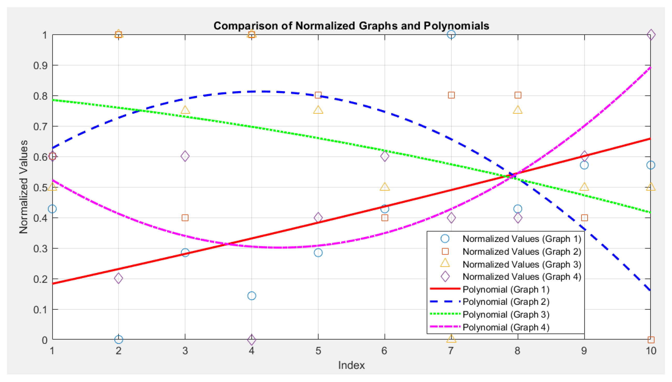
Figure 14 shows the graphical dependencies of the polynomial functions between the fifth and sixth groups, related to the correlation analysis.
The comparative analysis has shown that:
Correlation between Graph 1 and Graph 2: -0.03
Correlation between Graph 3 and Graph 4: -0.06
The value of -0.03 indicates a very weak or almost zero negative correlation. There is no significant relationship between the values of Graph 1 and Graph 2. They change independently of each other. The value of -0.06 also indicates an almost zero negative correlation. The values of Graph 3 and Graph 4 are not significantly related, although a very slight inverse trend can be observed.
However, based on the graph availability levels, distinct trends are observed between these two levels, as indicated in the analysis of the specific groups presented above.
Figure 15 Graphical dependencies of the polynomial functions between the sixth and seventh groups, related to the correlation analysis.
Regarding the correlation coefficients, the following is obtained:
Correlation between Graph 1 and Graph 2: -0.36
Correlation between Graph 3 and Graph 4: -0.49
The value of -0.36 indicates a weak to moderate negative correlation. This means that when the value in Graph 1 increases, the value in Graph 2 decreases, and vice versa. However, the relationship is not very strong. The value of -0.49 indicates a moderate negative correlation. In this case, there is also an inverse relationship, but it is stronger compared to the first pair of graphs. When the value in Graph 3 increases, the values in Graph 4 generally increase as well, and vice versa.
However, based on the availability level of the graphs, distinct data trends are observed between these two levels, as indicated in the analysis of the specific groups presented above.
4. Conclusions
This study is focused on the development of a methodology based on machine learning for the analysis and assessment of risks in road traffic accidents involving pedestrians. The methodology offers a systematic and integrated approach for identifying key risk factors and examining their interactions within the transportation system - driver, vehicle, road, and environment. Through the structuring of linguistic variables and the use of modeling and forecasting algorithms, the methodology provides a mechanism for assessing the complex dependencies that influence road safety.
The obtained results highlight the importance of the human factor as a critical component of risk. Furthermore, the analysis reveals the potential for optimizing transportation infrastructure and vehicle technical systems as means for reducing risk.
The proposed methodology serves as a foundation for the development of decision-support systems aimed at improving road safety. Future prospects include expanding its application by integrating more extensive data, applying advanced analysis algorithms, and personalizing decisions based on the specific characteristics of different transportation systems.
Author Contributions
Conceptualization, H. U and P. M.; methodology, H.U and P. M.; software, S.D.; data curation, V.U. All authors participated equally in the research. All authors have read and agreed to the published version of the manuscript.
Funding
Please add The APC was founded by the Scientific and Research Sector of the Technical University of Sofia, Bulgaria.
Data Availability Statement
Not applicable.
Acknowledgments
This scientific publication is funded under the project "Improvement of Research Capacity and Quality for International Recognition and Sustainability of Sofia University of Technology" with contract number BG-RRP-2.004.0005, implemented within the framework of the National Research Infrastructure (NRI) at Sofia University of Technology by scientific group 3.4.14 "Development of a Cloud-Based Research Infrastructure Platform for Innovative Technologies in Road Safety." We express our sincere gratitude for the support and assistance provided.
Conflicts of Interest
The authors declare no conflict of interest.
References
- Abdel-Aty, M.; Lee, J.; Yu, R. Analysis of pedestrian crashes using machine learning algorithms. Accident Analysis & Prevention 2019, 131, 285–293. [Google Scholar]
- Zhang, G.; Yau, K. K. W.; Chen, G. Risk factors associated with traffic violations and accident severity in China. Accident Analysis & Prevention 2016, 95, 503–511. [Google Scholar]
- Delen, S.; Sharda, R.; Bessonov, M. Identifying significant predictors of injury severity in traffic accidents using a series of artificial neural networks. Accident Analysis & Prevention 2006, 38, 434–444. [Google Scholar]
- He, H.; Garcia, E. A. Learning from imbalanced data. IEEE Transactions on Knowledge and Data Engineering 2009, 21, 1263–1284. [Google Scholar] [CrossRef]
- Yassin, S. S.; Pooja. Road accident prediction and model interpretation using a hybrid K-means and random forest algorithm approach. SN Applied Sciences 2020, 2, 1–13. [CrossRef]
- Hanna, C. L.; Hasselberg, M.; Laflamme, L.; Möller, J. Road traffic crash circumstances and consequences among young unlicensed drivers: A Swedish cohort study on socioeconomic disparities. BMC Public Health 2010, 10, 14. [Google Scholar] [CrossRef] [PubMed]
- Alkheder, S.; Taamneh, M.; Taamneh, S. Severity prediction of traffic accident using an artificial neural network. Journal of Forecasting 2017, 36, 100–108. [Google Scholar] [CrossRef]
- Rezapour, M.; Mehrara Molan, A.; Ksaibati, K. Analyzing injury severity of motorcycle at-fault crashes using machine learning techniques, decision tree and logistic regression models. International Journal of Transportation Science and Technology 2020, 9, 89–99. [Google Scholar] [CrossRef]
- Jamal, A.; Umer, W. Exploring the injury severity risk factors in fatal crashes with neural network. International Journal of Environmental Research and Public Health 2020, 17, 7466. [Google Scholar] [CrossRef]
- Chen, X.; Zhang, Y.; Zhu, Z.; Wang, J. Real-time pedestrian detection and tracking for intelligent transportation systems using deep learning. Transportation Research Part C: Emerging Technologies 2020, 111, 62–78. [Google Scholar] [CrossRef]
- Labib, M. F.; Rifat, A. S.; Hossain, M. M.; Das, A. K.; Nawrine, F. Road Accident Analysis and Prediction of Accident Severity by Using Machine Learning in Bangladesh. In Proceedings of the 7th International Conference on Smart Computing and Communication, ICSCC 2019, pp. 7–11, 2019. [CrossRef]
- Mokhtarimousavi, S.; Anderson, J. C.; Azizinamini, A.; Hadi, M. Improved Support Vector Machine Models for Work Zone Crash Injury Severity Prediction and Analysis. Transportation Research Record 2019, 2673, 680–692. [Google Scholar] [CrossRef]
- Rajkumar, A. R.; Prabhakar, S.; Priyadharsini, A. M. Prediction of road accident severity using machine learning algorithm. International Journal of Advanced Science and Technology 2020, 29, 116–120. [Google Scholar]
- Chen, M. M.; Chen, M. C. Modeling road accident severity with comparisons of logistic regression, decision tree and random forest. Information 2020, 11, 270. [Google Scholar] [CrossRef]
- Friedman, J. H. Greedy function approximation: A gradient boosting machine. Annals of Statistics 2001, 29, 1189–1232. [Google Scholar] [CrossRef]
- Mannering, F. L.; Shankar, V.; Bhat, C. R. Unobserved heterogeneity and the statistical analysis of highway accident data. Analytic Methods in Accident Research 2016, 11, 1–16. [Google Scholar] [CrossRef]
- Sharafaldin, I.; Lashkari, A. H.; Ghorbani, A. A. A detailed analysis of the CICIDS2017 data set. In Proceedings of the Information Systems Security and Privacy, pp. 172–188. Springer, 2018. [CrossRef]
- He, H.; Garcia, E. A. Learning from imbalanced data. IEEE Transactions on Knowledge and Data Engineering 2009, 21, 1263–1284. [Google Scholar] [CrossRef]
- Al Lail, M.; Garcia, A.; Olivo, S. Machine learning for network intrusion detection—a comparative study. Future Internet 2023, 15, 243. [Google Scholar] [CrossRef]
- Yin, C.; Zhu, Y.; Fei, J.; He, X. A deep learning approach for intrusion detection using recurrent neural networks. IEEE Access 2017, 5, 21954–21961. [Google Scholar] [CrossRef]
- Panigrahi, R.; Borah, S. A detailed analysis of CICIDS2017 dataset for designing intrusion detection systems. International Journal of Engineering and Technology 2018, 7, 479–482. [Google Scholar] [CrossRef]
- Maseer, Z. K.; Yusof, R.; Bahaman, N.; Mostafa, S. A.; Foozy, C. F. M. Benchmarking of machine learning for anomaly-based intrusion detection systems in the CICIDS2017 dataset. IEEE Access 2021, 9, 22351–22370. [Google Scholar] [CrossRef]
- Hashmienejad, S. H.-A.; Hasheminejad, S. M. H. Traffic accident severity prediction using a novel multi-objective genetic algorithm. International Journal of Crashworthiness 2017, 22, 425–440. [Google Scholar] [CrossRef]
- Breiman, L. Random forests. Machine Learning 2001, 45, 5–32. [Google Scholar] [CrossRef]
- Delen, D.; Sharda, R.; Bessonov, M. Identifying significant predictors of injury severity in traffic accidents using a series of artificial neural networks. Accident Analysis & Prevention 2006, 38, 434–444. [Google Scholar]
- Tang, J.; Liu, F.; Zou, Y.; Zhang, W.; Wang, Y. An improved fuzzy neural network for traffic speed prediction considering periodic characteristic. IEEE Transactions on Intelligent Transportation Systems 2017, 18, 2340–2350. [Google Scholar] [CrossRef]
Figure 1.
Transportation system: driver, vehicle, road, and environment.
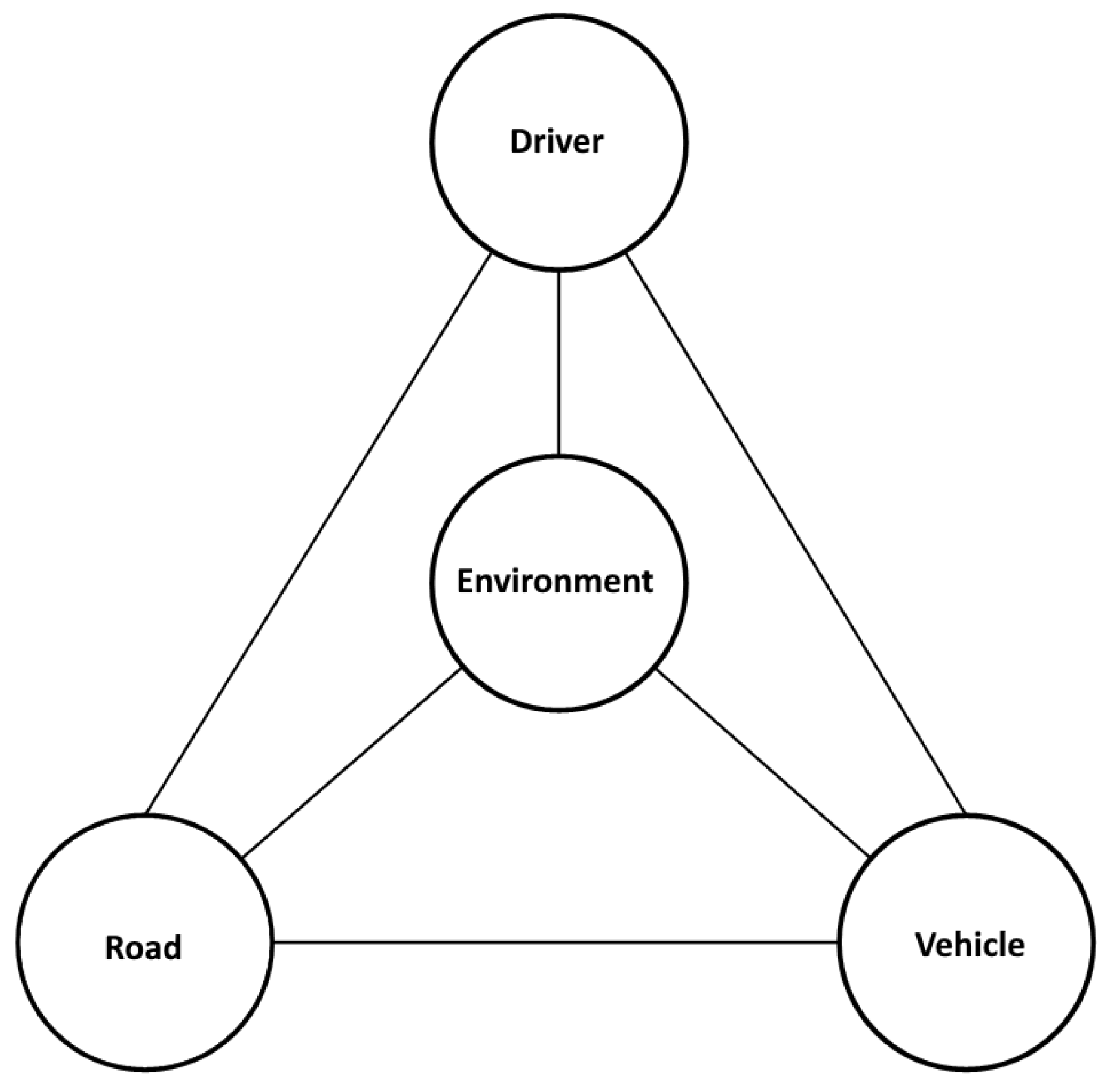
Figure 2.
Diagram of the system: driver, vehicle, road, and environment.
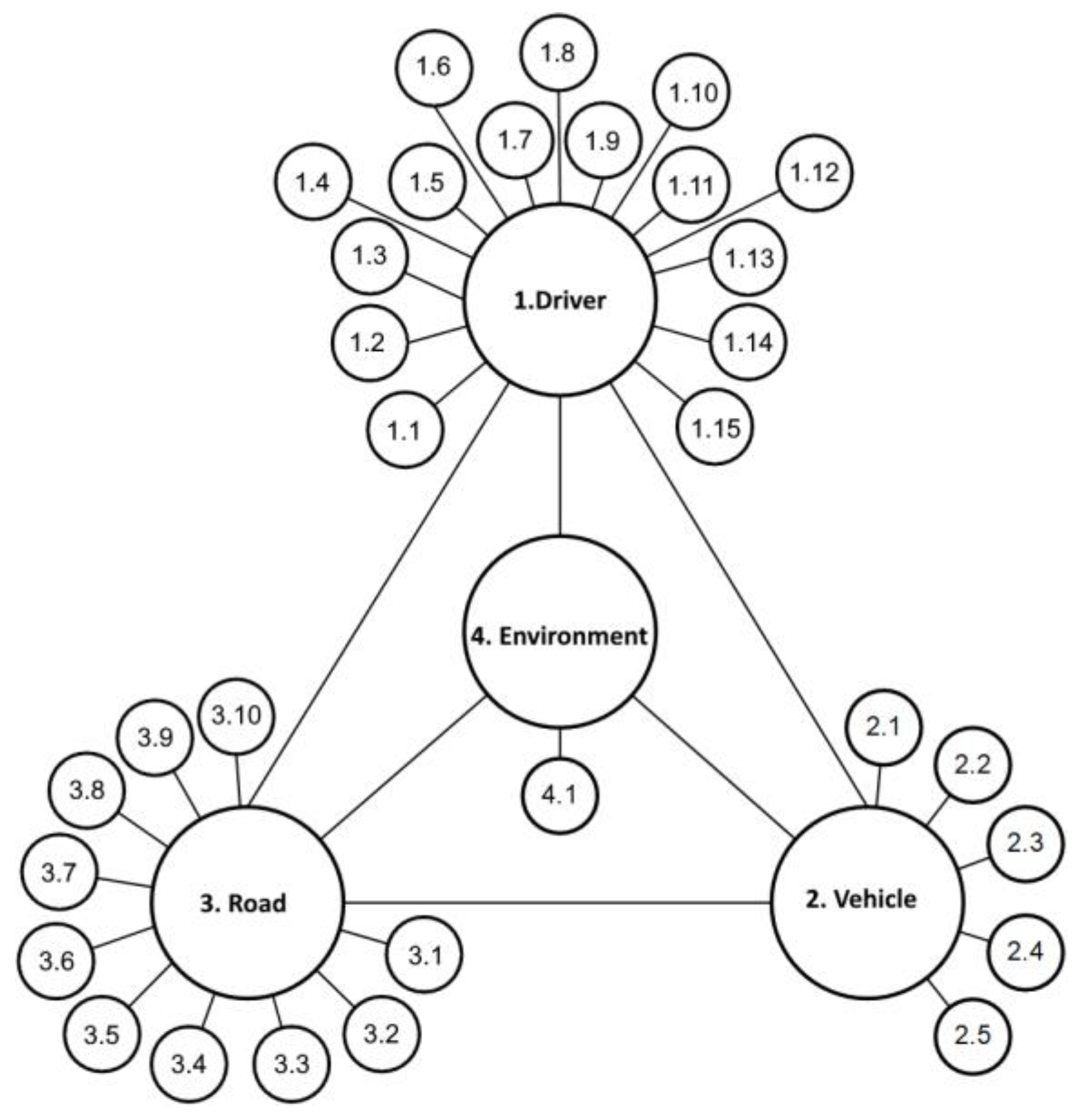
Figure 3.
Pie chart of weighted units up to 38.86% for the "road-vehicle" and "driver" components: (a) Levels of weights for the elements "road" and "vehicle"; (b) Driver's behavior.
Figure 3.
Pie chart of weighted units up to 38.86% for the "road-vehicle" and "driver" components: (a) Levels of weights for the elements "road" and "vehicle"; (b) Driver's behavior.
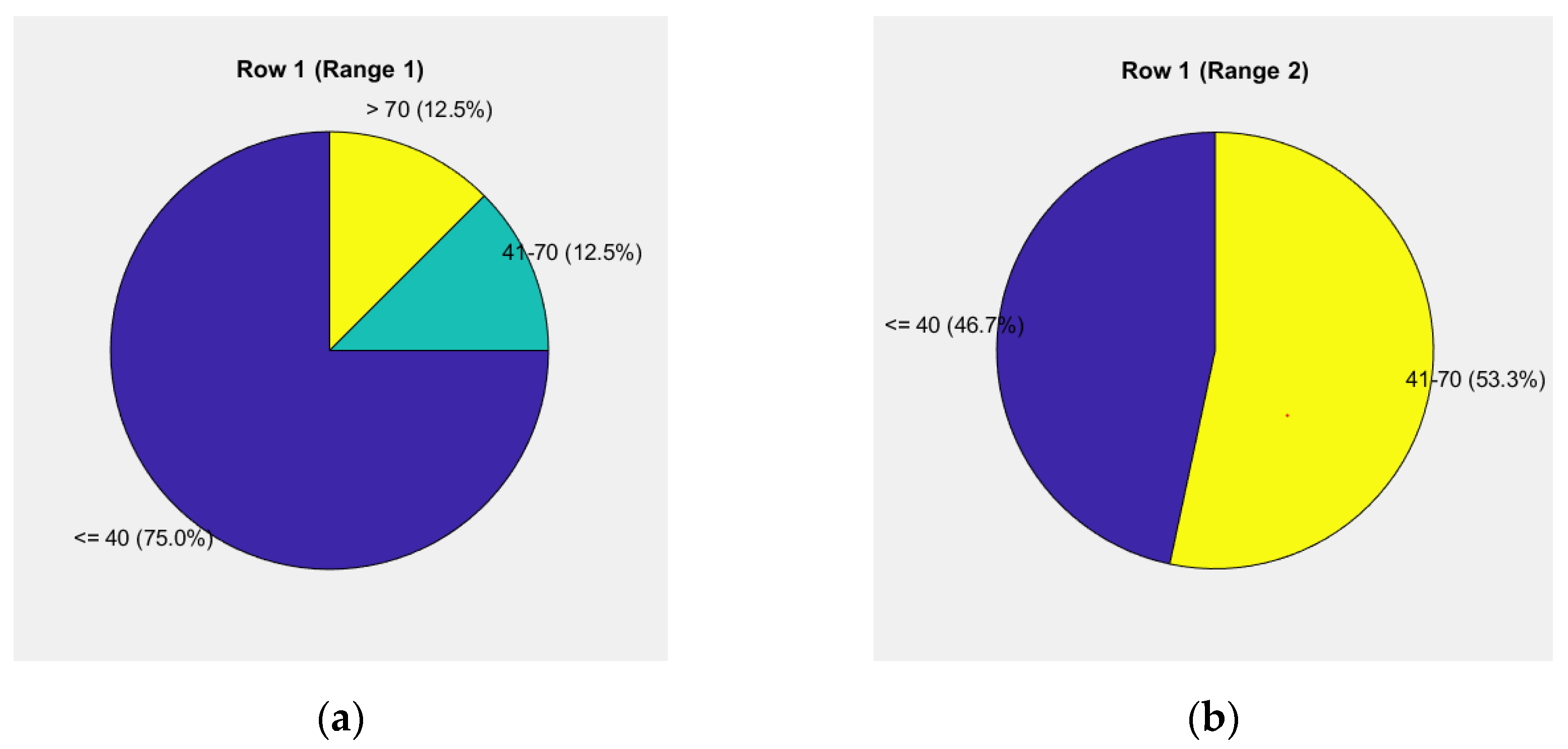
Figure 4.
Pie chart of weighted units up to 45.05% for the "road-vehicle" and "driver" components: (a) Levels of weights for the elements "road" and "vehicle"; (b) Driver's behavior.
Figure 4.
Pie chart of weighted units up to 45.05% for the "road-vehicle" and "driver" components: (a) Levels of weights for the elements "road" and "vehicle"; (b) Driver's behavior.
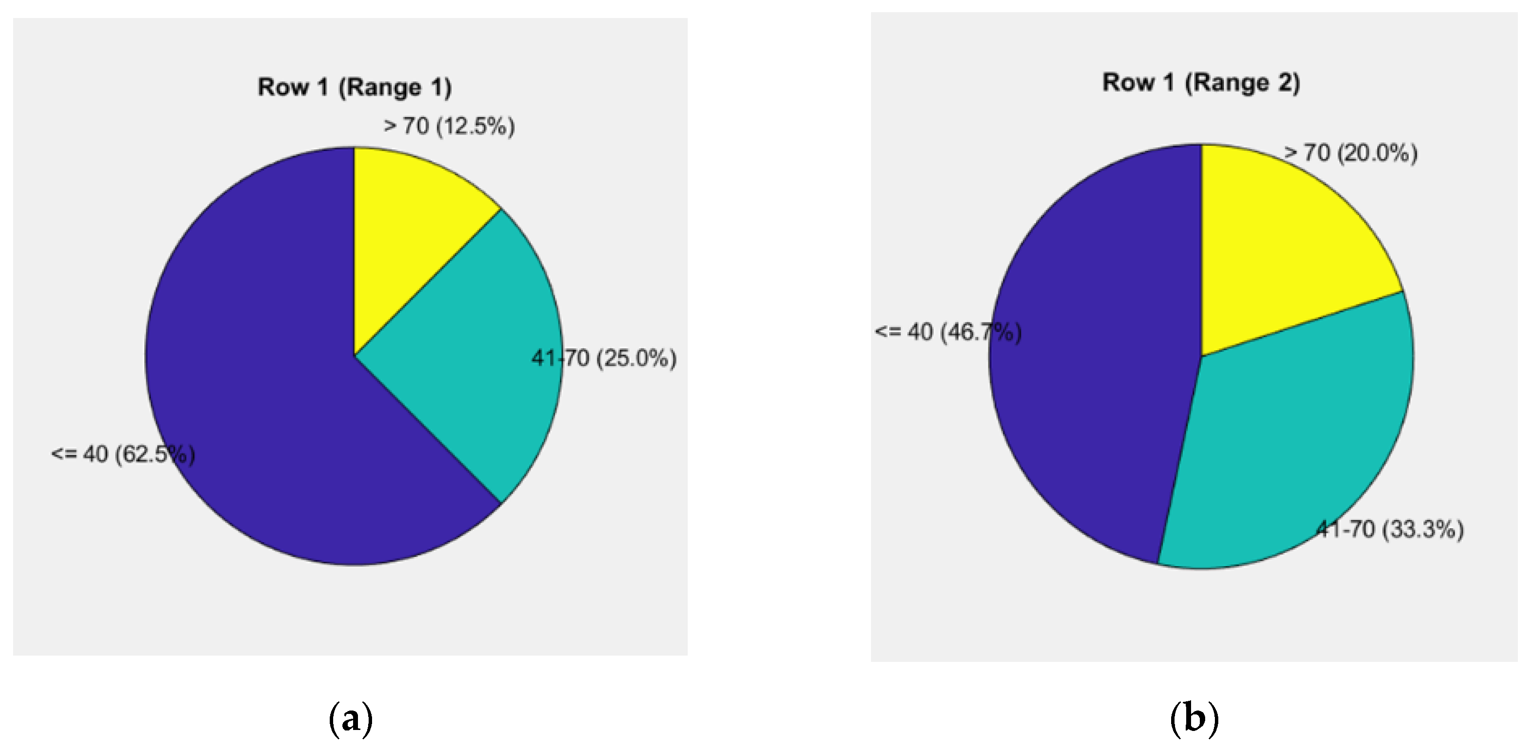
Figure 5.
Pie chart of weighted units up to 47.27% for the "road-vehicle" and "driver" components: (a) Levels of weights for the elements "road" and "vehicle"; (b) Driver's behavior.
Figure 5.
Pie chart of weighted units up to 47.27% for the "road-vehicle" and "driver" components: (a) Levels of weights for the elements "road" and "vehicle"; (b) Driver's behavior.
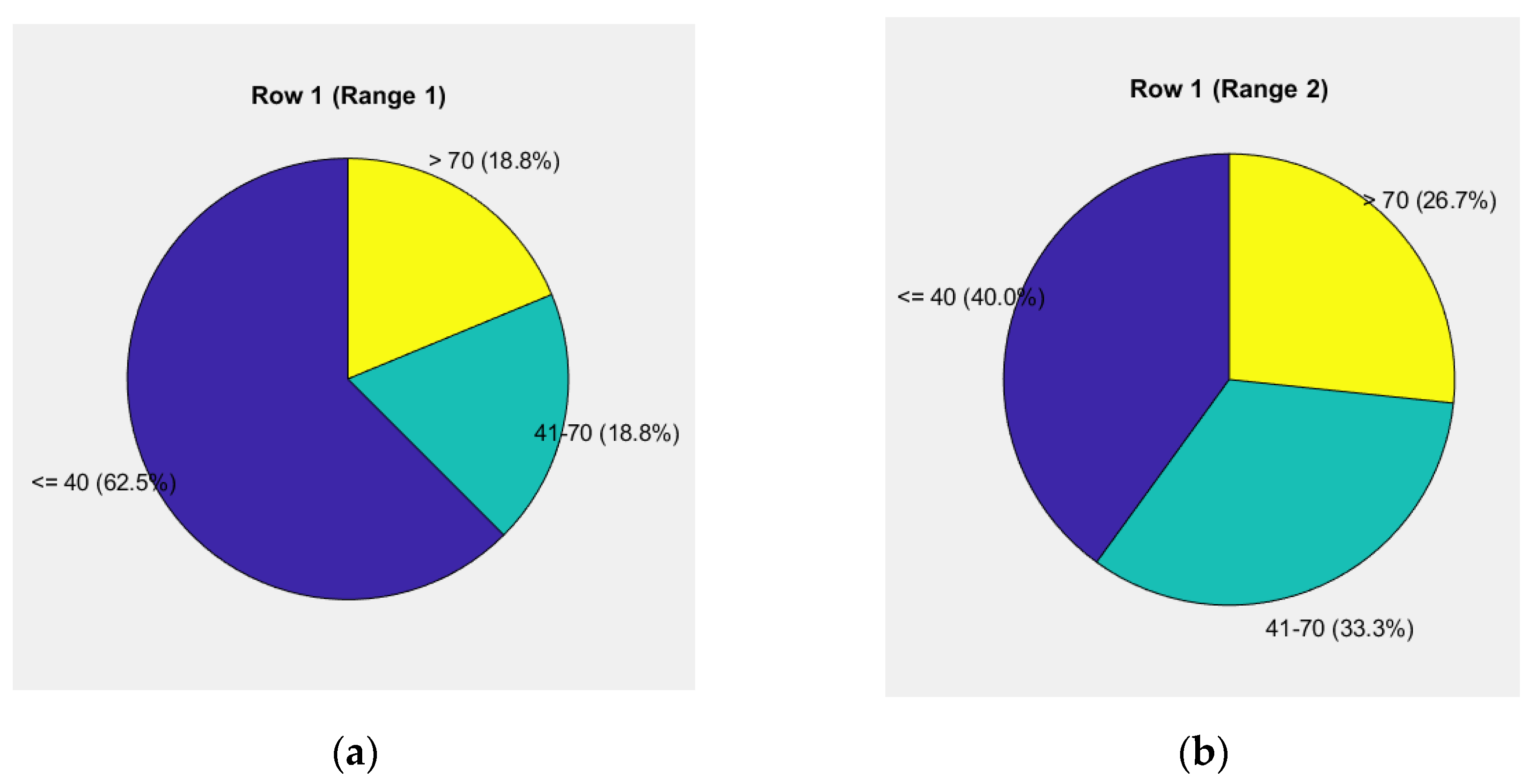
Figure 6.
Pie chart of weighted units up to 49.29% for the "road-vehicle" and "driver" components: (a) Levels of weights for the elements "road" and "vehicle"; (b) Driver's behavior.
Figure 6.
Pie chart of weighted units up to 49.29% for the "road-vehicle" and "driver" components: (a) Levels of weights for the elements "road" and "vehicle"; (b) Driver's behavior.
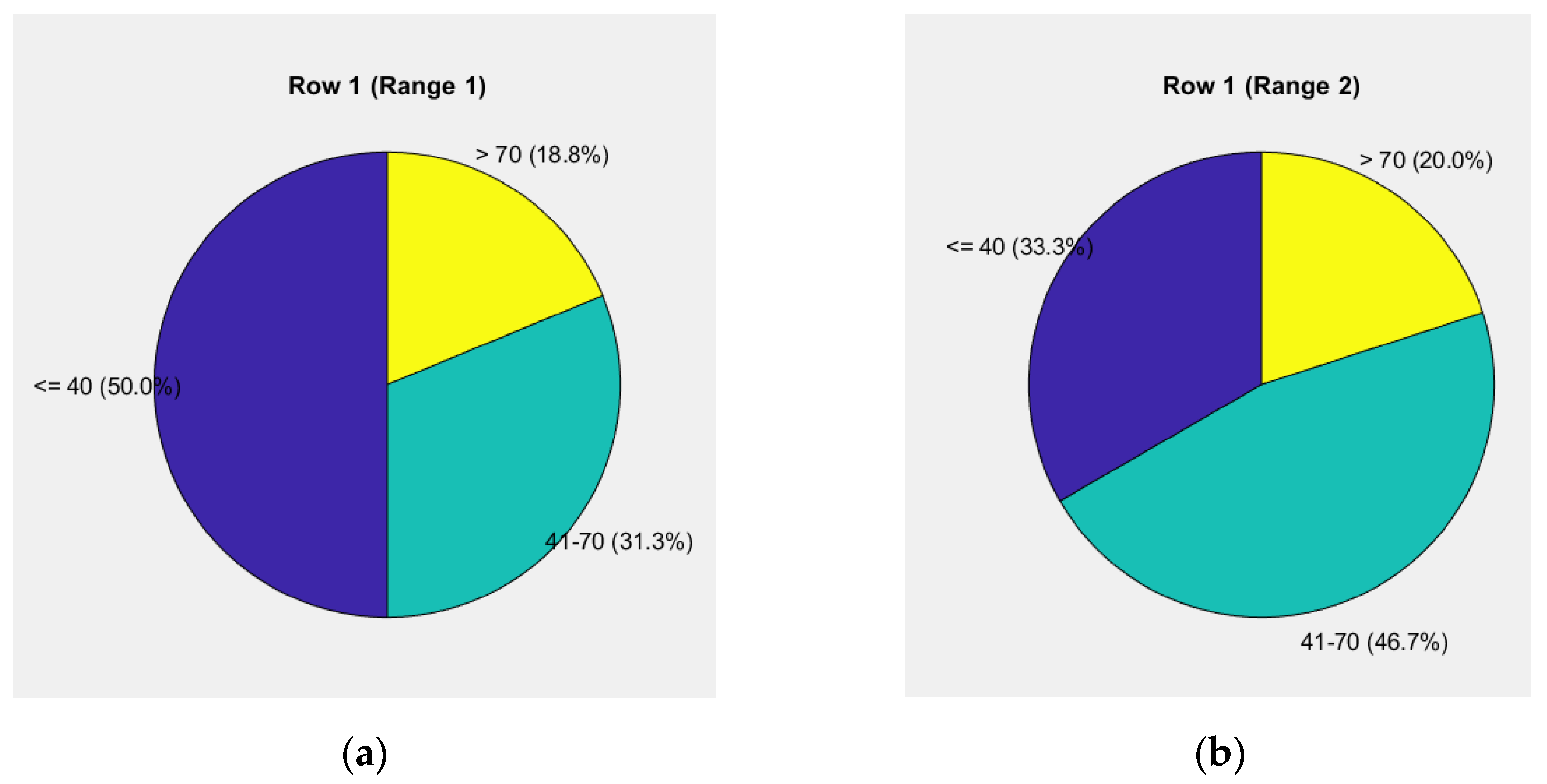
Figure 7.
Pie chart of weighted units up to 50.88% for the "road-vehicle" and "driver" components: (a) Levels of weights for the elements "road" and "vehicle"; (b) Driver's behavior.
Figure 7.
Pie chart of weighted units up to 50.88% for the "road-vehicle" and "driver" components: (a) Levels of weights for the elements "road" and "vehicle"; (b) Driver's behavior.
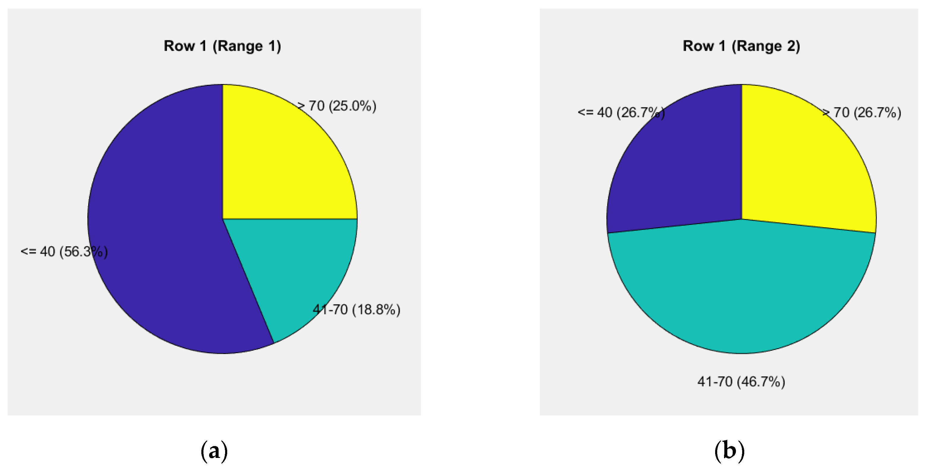
Figure 8.
Pie chart of weighted units up to 53.65% for the "road-vehicle" and "driver" components: (a) Levels of weights for the elements "road" and "vehicle"; (b) Driver's behavior.
Figure 8.
Pie chart of weighted units up to 53.65% for the "road-vehicle" and "driver" components: (a) Levels of weights for the elements "road" and "vehicle"; (b) Driver's behavior.
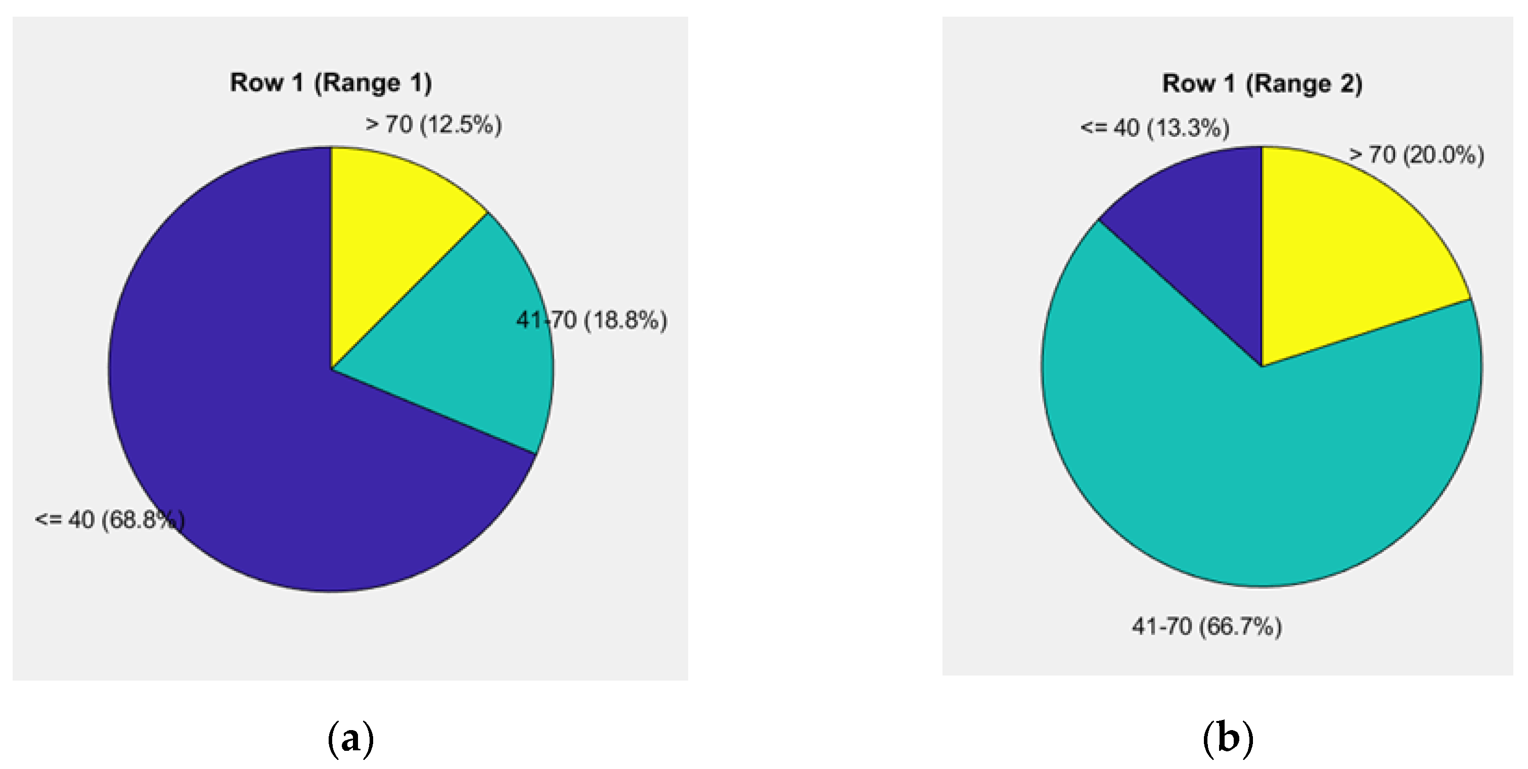
Figure 9.
Pie chart of weighted units up to 55.24% for the "road-vehicle" and "driver" components: (a) Levels of weights for the elements "road" and "vehicle"; (b) Driver's behavior.
Figure 9.
Pie chart of weighted units up to 55.24% for the "road-vehicle" and "driver" components: (a) Levels of weights for the elements "road" and "vehicle"; (b) Driver's behavior.
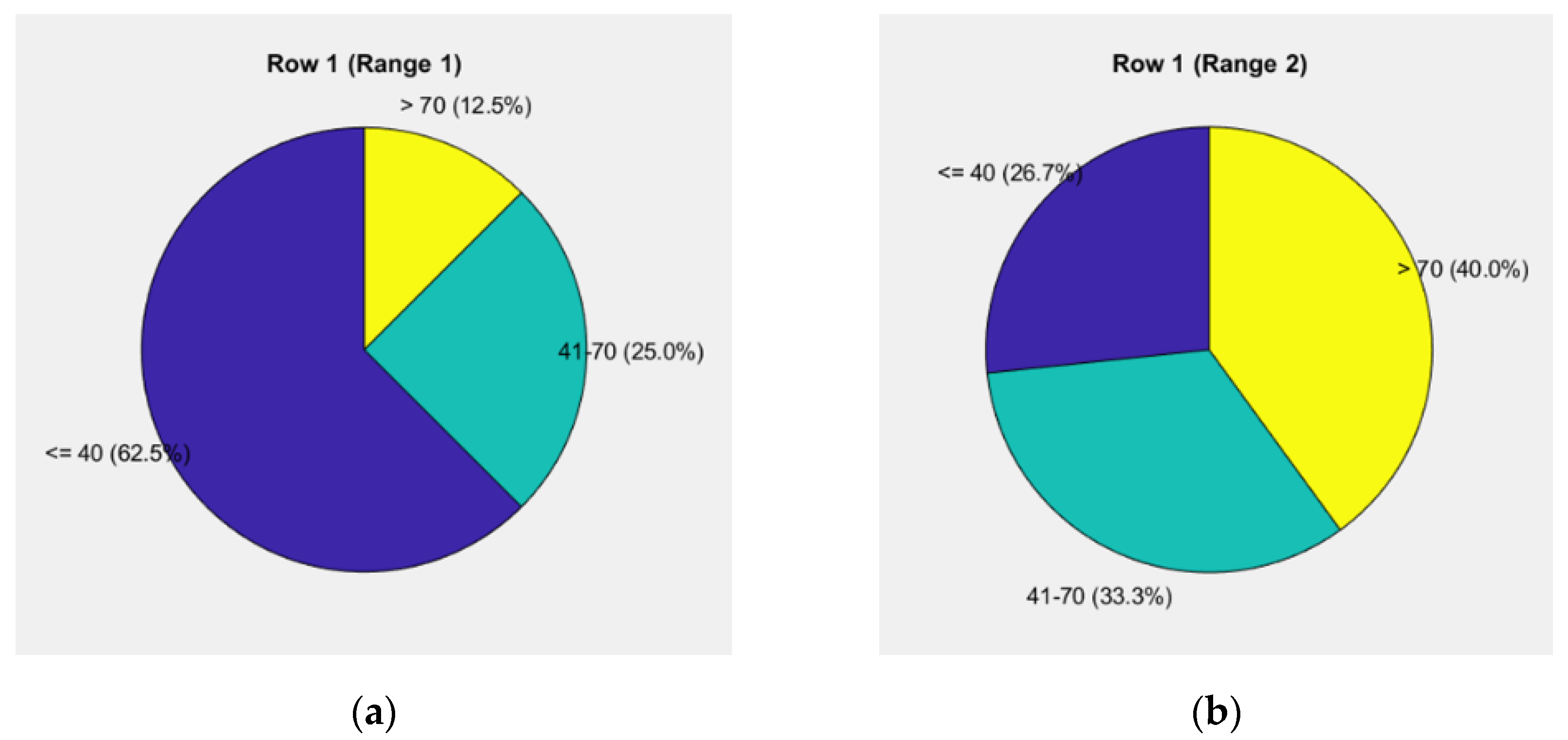
Figure 10.
Pie chart of weighted units up to 58.35% for the "road-vehicle" and "driver" components: (a) Levels of weights for the elements "road" and "vehicle"; (b) Driver's behavior.
Figure 10.
Pie chart of weighted units up to 58.35% for the "road-vehicle" and "driver" components: (a) Levels of weights for the elements "road" and "vehicle"; (b) Driver's behavior.
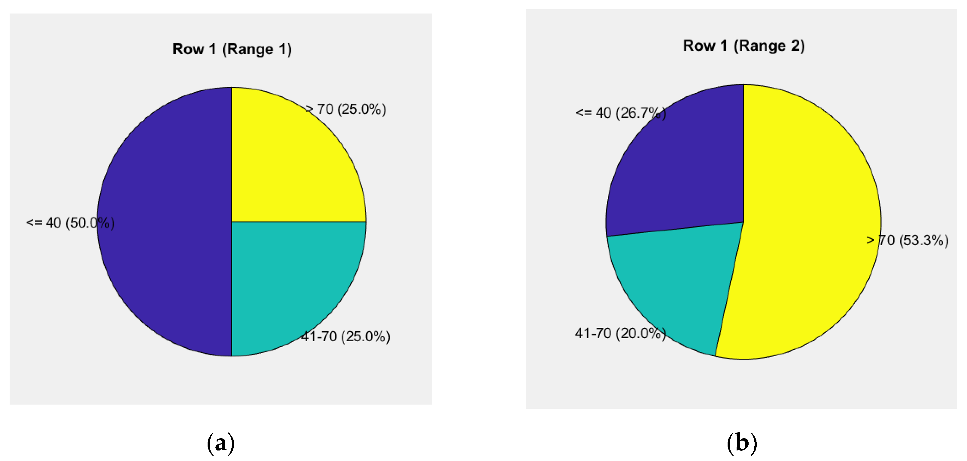
Figure 11.
Pie chart of weighted units up to 62.59% for the "road-vehicle" and "driver" components: (a) Levels of weights for the elements "road" and "vehicle"; (b) Driver's behavior.
Figure 11.
Pie chart of weighted units up to 62.59% for the "road-vehicle" and "driver" components: (a) Levels of weights for the elements "road" and "vehicle"; (b) Driver's behavior.
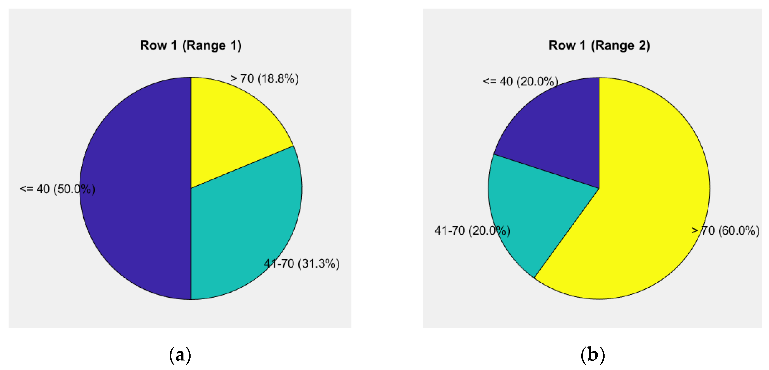
Figure 12.
Graphical dependencies of the polynomial functions between the third and fourth groups.
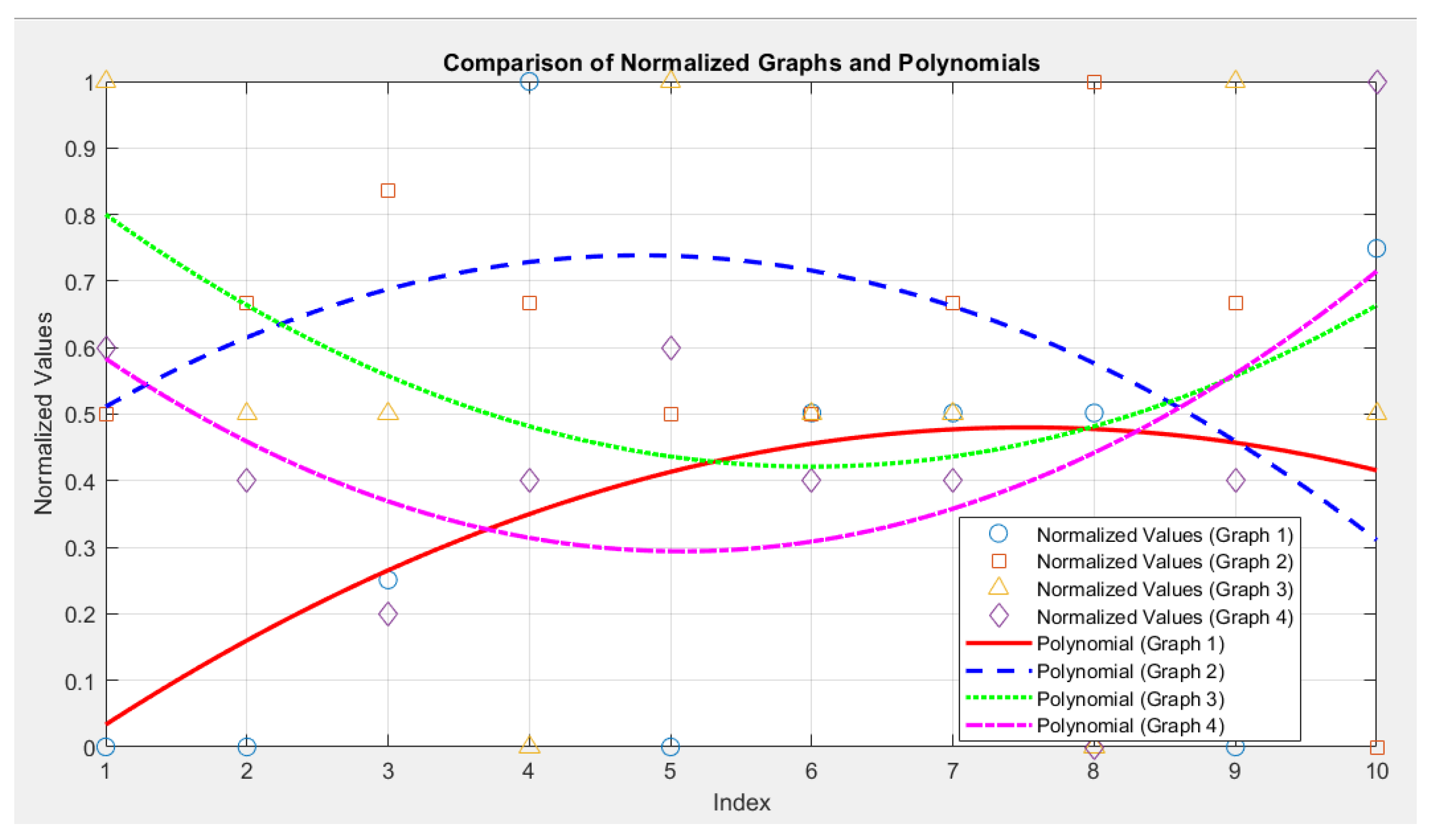
Figure 13.
Graphical dependencies of the polynomial functions between the third and fourth groups.
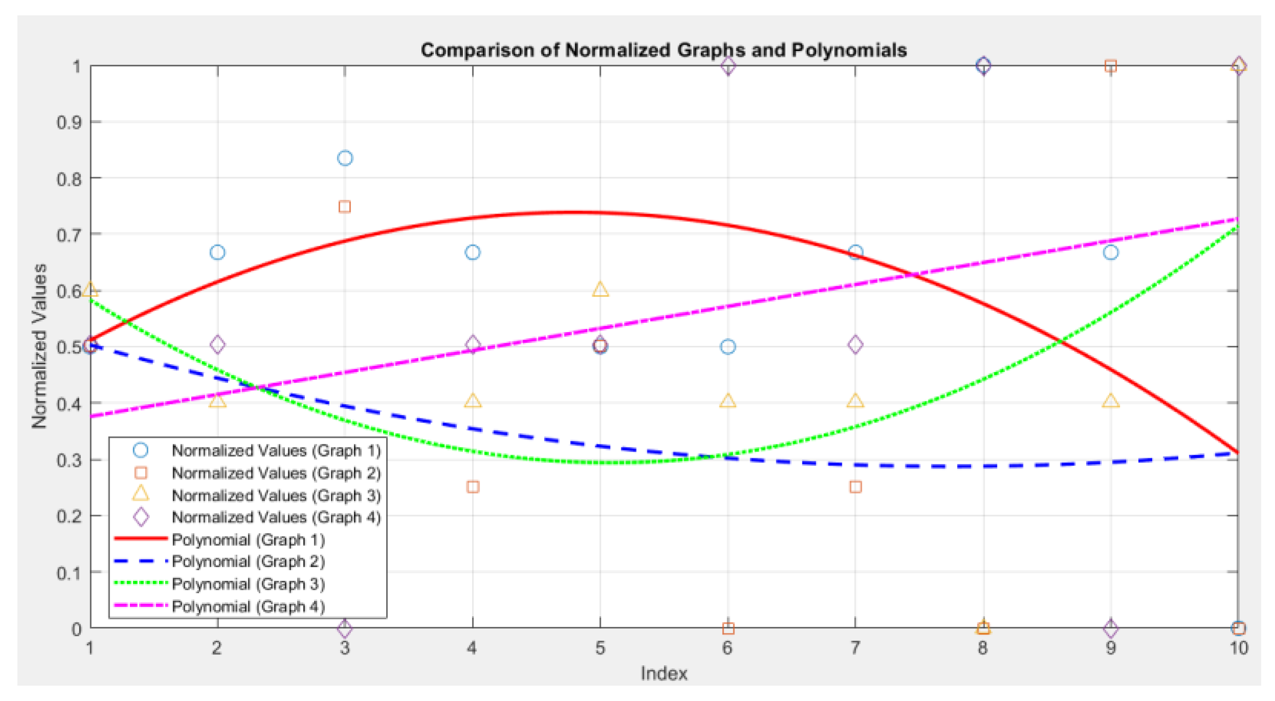
Figure 14.
Graphical dependencies of the polynomial functions between the fifth and sixth groups, related to the correlation analysis.
Figure 14.
Graphical dependencies of the polynomial functions between the fifth and sixth groups, related to the correlation analysis.
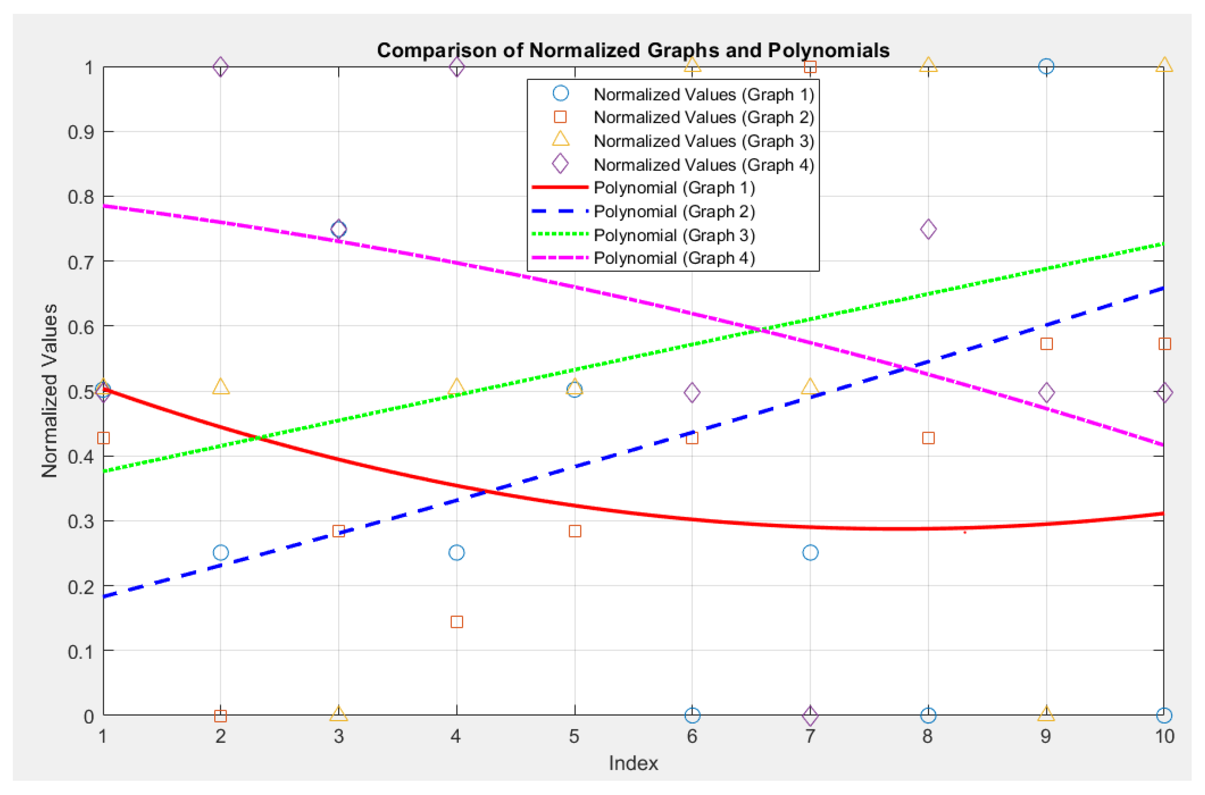
Figure 15.
Graphical dependencies of the polynomial functions between the sixth and seventh groups.
Disclaimer/Publisher’s Note: The statements, opinions and data contained in all publications are solely those of the individual author(s) and contributor(s) and not of MDPI and/or the editor(s). MDPI and/or the editor(s) disclaim responsibility for any injury to people or property resulting from any ideas, methods, instructions or products referred to in the content. |
© 2024 by the authors. Licensee MDPI, Basel, Switzerland. This article is an open access article distributed under the terms and conditions of the Creative Commons Attribution (CC BY) license (http://creativecommons.org/licenses/by/4.0/).
Copyright: This open access article is published under a Creative Commons CC BY 4.0 license, which permit the free download, distribution, and reuse, provided that the author and preprint are cited in any reuse.


