Submitted:
02 January 2025
Posted:
07 January 2025
You are already at the latest version
Abstract
This This study presents a comparative analysis of two methodologies for predicting the risk of pedestrian-involved traffic accidents. The methodologies examined include one based on proportional risk distribution and another employing the machine learning algorithm Random Forest. The primary objective is to evaluate the applicability and accuracy of the proposed approaches through the processing and analysis of data derived from real-world cases of concluded legal proceedings. Linguistic variables, defined as risk factors, are classified and quantified based on expert evaluations. The results include interpolation models and graphical representations illustrating the risk severity according to the two methodologies. The analysis demonstrates that both methodologies are applicable for risk assessment, with the Random Forest algorithm providing superior accuracy and reliability in processing complex and heterogeneous data. Furthermore, a correlation analysis confirms a statistically significant linear relationship between the results of the two approaches. Visualization of the results through various graphical tools supports an objective comparison of the methodologies and their application in transport safety analysis.
Keywords:
traffic accidents
; risk
; machine learning
; random forest
; proportional distribution
; linguistic variables
; correlation analysis
; transport safety
; prediction
; interpolation
1. Introduction
Pedestrian-involved traffic accidents represent a significant social and public health issue, leading to a substantial number of fatalities and severe injuries. Preventing such incidents necessitates the development of effective and innovative risk prediction approaches that integrate the complex dynamics and interdependencies of multiple factors. Machine learning has proven to be a reliable method for processing large datasets and predicting risk-related events, including pedestrian accidents [1,2,3].
The complex informational processes underlying the causes of traffic accidents, as well as the interdependencies between factors such as infrastructure, human behavior, and weather conditions, position machine learning as a cornerstone in the analysis and modeling of transportation systems. Traditional analytical methods often prove insufficient in capturing this complexity, making machine learning algorithms indispensable tools for risk assessment and prediction.
Studies by Theofilatos and Yannis [4], as well as Peng et al. [5], highlight that the interaction between traffic flow and weather conditions plays a crucial role in evaluating the risk of traffic accidents. The ability of these algorithms to process large volumes of data, handle imperfect or incomplete inputs, and identify complex dependencies underscores their applicability in assessing pedestrian-involved traffic accident risk [6].
Among these algorithms are Random Forest, Decision Tree, Support Vector Machines (SVM), Neural Networks, and others, which primarily differ in their training methodologies. Machine Learning (ML) relies on the availability of well-structured and properly annotated data that can be used to develop highly accurate models. In this context, the data and its structure are key components for the effective application of ML algorithms. The effectiveness of ML depends not only on the algorithms themselves but also on the quality and organization of the data. The studies by Mokhtarimousavi et al. demonstrate that improved Support Vector Machine models are highly effective for predicting the severity of incidents in work zones [7].
This study proposes a novel methodology for assessing the risk of pedestrian-involved traffic accidents, which is comparable to methods based on machine learning algorithms. The proposed methodological approach is founded on the distribution of weights assigned to factors contributing to such accidents, determined by their relative significance within the analyzed system. A comparative analysis was conducted between the risk assessments generated by the proposed methodology and the results obtained using the Random Forest algorithm.
The primary objective of the study is to validate the applicability of the proposed new methodology for predicting the risk of pedestrian-involved traffic accidents through a correlation analysis of the obtained results.
2. Methodology
Predicting the risk of pedestrian-involved traffic accidents requires the integration and processing of heterogeneous data that reflect various aspects of the transportation system and the interactions among its components [8,9]. The Random Forest algorithm is widely used for analyzing factors influencing traffic accident risk due to its robustness and accuracy [10,11]. In the analysis of such data, an imbalance between classes is often observed, where rare events such as severe accidents are underrepresented. Techniques such as Random Forest and handling of imbalanced data are applied to address this issue, significantly improving model accuracy [12].
Studies have shown that neural networks can successfully predict the severity of accidents by utilizing parameters such as driver and pedestrian behavior [13,14,15]. This capability makes them well-suited for analyzing the complex and heterogeneous data characteristic of transportation systems.
The transportation system is a complex multi-component structure in which interactions among drivers, vehicles, road infrastructure, and the environment generate diverse data [16]. The effective application of data-driven approaches for predicting the risk of pedestrian-involved traffic accidents requires methodical and well-founded data preparation [17,18]. This process involves detailed structuring and classification of data, which are essential for identifying patterns and establishing dependencies that determine traffic safety.
2.1. Data Classification and Structuring
The data sources for this study include case files, judicial rulings, and technical expert analyses derived from concluded legal proceedings related to pedestrian-involved traffic accidents. A key aspect of data classification is their distribution across the main elements of the transportation system: driver, vehicle, road, and environment (Figure 1).
Within the framework of this study, the key factors influencing the risk of pedestrian-involved traffic accidents have been identified. These factors are interpreted as linguistic variables, representing essential aspects of the transportation system in the context of safety. Similar factors, such as driver behavior, infrastructure, and environmental conditions, have been recognized as primary risk contributors in other studies, such as the analysis of violations and accident severity in China [19].
For each linguistic variable, values representing qualitative descriptions, known as terms, have been defined. Each term is associated with a risk influence scale expressed as percentage values, ranging from 10% to 90%, based on expert evaluations. The linguistic variables are designated in Figure 1 as follows:
- Driver: Variables 1.1 to 1.15
- Vehicle: Variables 2.1 to 2.5
- Road: Variables 3.1 to 3.10
- Environment: Variable 4.1
The linguistic variables, their terms, and the percentage values indicating their influence on risk are presented as follows:
1 Driver Element:
1.1 Current Speed: “At or below the normalized speed” – 10%; “Exceeding the normalized speed by up to 10 km/h” – 40%; “Exceeding the normalized speed by up to 20 km/h” – 50%; “Exceeding the normalized speed by up to 30 km/h” – 60%; “Exceeding the normalized speed by up to 40 km/h” – 70%; “Exceeding the normalized speed by up to 50 km/h” – 80%; “Exceeding the normalized speed by more than 50 km/h” – 90%.
1.2 Maneuver: “Absence of improper maneuver” – 10%; “Improper use of lights” – 15%; “Failure to maintain distance” – 25%; “Improper stopping or parking” – 30%; “Improper passing” – 35%; “Improper lane change” – 40%; “Improper reversing” – 45%; “Improper right turn” – 50%; “Improper left turn” – 65%; “Improper U-turn” – 70%; “Sudden change of direction” – 80%; “Improper overtaking” – 85%; “Entering oncoming traffic” – 90%.
1.3 Alcohol and Drug Use by the Driver: “Absence of alcohol/drugs” – 20%; “Presence of alcohol/drugs up to 0.5‰” – 50%; “Presence of alcohol/drugs from 0.51 to 1.2‰” – 70%; “Presence of alcohol/drugs over 1.21‰” – 90%.
1.4 Driver Experience: “36 to 50 years /experienced driver/” – 20%; “11 to 35 years /moderately experienced driver/” – 30%; “Up to 10 years /young driver/” – 60%; “Over 51 years /elderly driver/” – 80%; “Inexperienced driver” – 90%.
1.5 Hazard Occurrence: “Movement on the sidewalk” – 10%; “Stationary on the sidewalk/bus stop” – 20%; “Playing/stationary on the roadway” – 30%; “Upon spotting an oncoming pedestrian on the roadway” – 40%; “Upon spotting a following pedestrian on the roadway” – 50%; “After entering the roadway/limited visibility” – 60%; “At the moment of entering the roadway” – 70%; “Before entering the roadway” – 80%; “Crossing the roadway along the continuation of the sidewalk” – 40%; “Crossing the roadway outside a pedestrian crossing” – 50%.
1.6 Pedestrian Behavior: “Crossing on a green light” – 20%; “Crossing the roadway at a pedestrian crossing” – 30%; “Moving in the same or opposite direction on the roadway” – 60%; “Stationary on the roadway” – 65%; “Emerging in front of/behind a vehicle” – 75%; “Crossing on a red light” – 80%; “Crossing or moving in the same/opposite direction involving children or elderly pedestrians” – 90%.
1.7 Hazard Perception: “Before the hazard occurs” – 30%; “At the moment the hazard occurs” – 40%; “After the hazard occurs, with a delay of up to 0.5 seconds” – 50%; “After the hazard occurs, with a delay of up to 1.0 second” – 60%; “After the hazard occurs, with a delay of up to 1.5 seconds” – 70%; “After the hazard occurs, with a delay of up to 2.0 seconds” – 80%; “After the hazard occurs, with a delay exceeding 2.1 seconds” – 90%.
1.8 Braking Initiation: “Braking initiated by the driver before the collision” – 50%; “Braking initiated by the driver after the collision” – 70%; “Leaving the scene of the accident by the driver” – 80%; “Driver falling asleep” – 90%.
1.9 Pedestrian Age: “56 to 70 years” – 10%; “31 to 55 years” – 20%; “17 to 30 years” – 40%; “Over 70 years” – 60%; “Up to 16 years” – 90%.
1.10 Movement Pace: “Stationary” – 10%; “Slow pace” – 30%; “Moderate pace” – 50%; “Fast pace” – 70%; “Steady running” – 80%; “Fast running” – 90%.
1.11 Alcohol and Drug Use by Pedestrian: “Absence of alcohol/drugs” – 30%; “Presence of alcohol/drugs up to 0.5‰” – 50%; “Presence of alcohol/drugs from 0.51 to 1.2‰” – 70%; “Presence of alcohol/drugs over 1.21‰ or mental impairment” – 90%.
1.12 Distance Comparison at Current Speed: “Stopping distance (SD) at current speed exceeds the distance to the collision point” – 40%; “SD at current speed equals the distance to the collision point” – 50%; “SD at current speed is less than the distance to the collision point” – 60%; “Collision during reverse motion (L=0 m)” – 70%.
1.13 Stopping Danger Zone at Current Speed: “Stopping danger zone (SDZ) at current speed is smaller than the distance to the collision point without deviation” – 40%; “SDZ at current speed is smaller than the distance to the collision point with deviation” – 50%; “Closing in during same or opposite direction movement” – 60%; “Closing in while leaving the roadway” – 70%.
1.14 Distance Comparison at Normalized Speed: “Stopping distance (SD) at normalized speed exceeds the distance to the collision point” – 40%; “SD at normalized speed equals the distance to the collision point” – 50%; “SD at normalized speed is smaller than the distance to the collision point” – 60%; “Collision during reverse motion (L=0 m)” – 70%.
1.15 Stopping Danger Zone at Normalized Speed: “Stopping danger zone (SDZ) at normalized speed is smaller than the distance to the collision point without deviation” – 40%; “SDZ at normalized speed is smaller than the distance to the collision point with deviation” – 50%; “Closing in during same or opposite direction movement” – 60%; “Closing in while leaving the roadway” – 70%.
In the classification of data within the “Driver” element, linguistic variables are included to represent both pedestrian characteristics (denoted as 1.9 to 1.11) and spatiotemporal dependencies (denoted as 1.12 to 1.15). This integration is justified by the systemic nature of the transportation system, where all elements—driver, vehicle, road, and environment—interact dynamically. Driver behavior cannot be considered in isolation, as it is strongly influenced by the actions of other traffic participants and environmental conditions.
Pedestrian characteristics are crucial for evaluating driver responses. For example, sudden crossings in prohibited areas, movements on the roadway, or unpredictable behavior by vulnerable participants such as children or elderly individuals significantly impact reaction time and the corrective actions taken. Furthermore, a pedestrian’s age, mobility, and potential use of alcohol or drugs determine the predictability of their behavior, which is a critical factor for the driver’s timely and adequate response.
Spatiotemporal dependencies also play a key role in assessing the risk of pedestrian-involved traffic accidents. They link driver behavior to the physical constraints of the system, such as current speed, the distance to a potential collision point, and the vehicle’s braking capabilities. Analyzing these dependencies allows for determining whether the driver could have avoided the incident through timely corrective actions. Evaluating the comparison between the distance to the collision point and the stopping danger zone is critically important, as it determines whether the accident could have been prevented under adherence to speed limits.
1. Vehicle Element:
1.1 Type of Vehicle: “Animal-drawn vehicle” – 10%; “Scooter” – 15%; “Bicycle” – 20%; “Moped” – 25%; “Motorcycle” – 30%; “Trolleybus” – 40%; “Special-purpose vehicle” – 50%; “Passenger car” – 60%; “Van (passenger and cargo)” – 65%; “Truck” – 70%; “Bus” – 75%; “Semi-trailer truck” – 80%; “Truck with trailer” – 90%.
1.2 Safety Systems: “Equipped with active safety systems (e.g., ABS, ESP)” – 20%; “Not equipped with active safety systems (e.g., ABS, ESP)” – 80%.
1.3 Lighting System – Control: “Adaptive” – 20%; “Standard” – 80%.
1.4 Lighting System – Type of Lights: “LED” – 20%; “Xenon” – 40%; “Halogen” – 70%.
1.5 Technical Condition: “Fully operational systems” – 10%; “Faulty lighting system” – 40%; “Faulty control devices” – 60%; “Faulty engine/transmission” – 70%; “Faulty suspension/steering” – 80%; “Faulty braking system” – 90%.
2 Road Element:
2.1 Road Surface Condition: “Dry” – 10%; “Wet” – 20%; “Muddy” – 30%; “Flooded” – 40%; “Melted snow” – 50%; “Snow (cleared)” – 60%; “Snow (uncleared)” – 70%; “Ice (cleared)/Frosty” – 80%; “Ice (uncleared)” – 90%.
2.2 Type of Road Surface: “Cement concrete” – 10%; “Asphalt concrete” – 20%; “Paved” – 30%; “Crushed stone surface” – 40%; “Dirt road” – 60%.
2.3 Traffic Flow Direction: “One-way” – 30%; “Two-way” – 70%.
2.4 Road Profile Plan: “Straight, flat section” – 10%; “Straight section with uphill gradient” – 20%; “Straight section with downhill gradient” – 25%; “Curve without gradient” – 30%; “Curve without gradient and positive superelevation” – 40%; “Curve without gradient and negative superelevation” – 50%; “Curve with gradient and positive superelevation” – 60%; “Curve with gradient and negative superelevation” – 70%; “Concave curve section” – 80%; “Convex curve section” – 90%.
2.5 Accident Location: “Pedestrian underpass/overpass” – 10%; “Bridge with sidewalks” – 15%; “Bridge without sidewalks” – 20%; “Parking area” – 25%; “Roadway section” – 30%; “Narrowed section or under repair” – 40%; “Tunnel” – 50%; “Pedestrian crossing including sidewalk continuation” – 60%; “School or childcare facility” – 70%; “Interchange” – 80%; “Intersection” – 90%.
2.6 Roadway Width: “Over 10.5 m” – 10%; “From 7.5 m to 10.5 m” – 20%; “From 7 m to 7.5 m” – 30%; “From 6 m to 7 m” – 40%; “Up to 6 m” – 50%.
2.7 Road Conditions: “Normal surface, visibility, and signaling” – 10%; “Insufficient horizontal and vertical markings” – 20%; “Insufficient visibility due to vegetation” – 30%; “Insufficient visibility due to roadside objects” – 40%; “Damaged road surface” – 50%; “Road surface irregularities” – 60%; “Obstacle on the roadway” – 70%.
2.8 Lighting Conditions: “Daylight” – 10%; “Artificial lighting” – 40%; “Dusk” – 60%; “Darkness” – 80%.
2.9 Traffic Regulation Conditions: “Traffic officer” – 10%; “Traffic light” – 50%; “Road signs” – 60%; “Flashing yellow light” – 70%; “Traffic rules” – 80%.
2.10 Road Class: “Highway” – 30%; “First-class road” – 40%; “Second-class road” – 50%; “Municipal road outside a settlement” – 60%; “Municipal road within a settlement” – 70%; “Third-class road” – 80%.
3 Environment Element:
3.1 Weather Conditions: “Clear” – 10%; “Cloudy” – 20%; “Rain” – 30%; “Fog with visibility over 200 m” – 40%; “Fog with visibility from 150 m to 199 m” – 50%; “Fog with visibility from 100 m to 149 m” – 60%; “Fog with visibility from 50 m to 99 m” – 65%; “Fog with visibility under 49 m or glare” – 70%; “Snowfall” – 75%; “Heavy rain” – 80%; “Strong wind” – 85%; “Hail” – 90%.
2.2. Methodology for Predicting the Risk of Pedestrian-Involved Traffic Accidents Based on Factor Weighting by Relative Importance
Based on a comprehensive analysis of case files, judicial rulings, expert evaluations from concluded legal proceedings, and statistical data, the proportional weighting of risk across different elements of the transportation system can be determined. The proposed methodology is founded on the principle of proportional distribution of the risk of pedestrian-involved traffic accidents among the contributing factors. Studies indicate that neural networks can effectively predict the severity of incidents by leveraging parameters such as driver and pedestrian behavior [20].
Assuming that the total risk weight for this type of traffic incident equals 100%, the distribution is conducted across the following three groups:
- Road and Environment Elements: 20% of the value for each term of the respective linguistic variables.
- Vehicle Element: 10% of the value for the terms of the linguistic variables.
- Driver Element: 70% of the value for the terms of the linguistic variables.
This distribution can be represented as a vector of target values for each group:
This approach provides an objective framework for the quantitative assessment of the relative risk weight associated with individual elements of the transportation system. The input data for the proposed methodology is a vector consisting of values for 31 linguistic variables represented through the weights of the terms described in Section 2.1. The vector characterizes a specific pedestrian-involved traffic accident case.
where , are numerical values representing the relative weight of each term in the array .
The weighted average risk value for each term within the groups can be determined using the following expression:
where:
is the weighted risk value for the -th term in group ;
is the sum of all term weights by index ;
is the target value of the -th element in vector ;
for , .
The difference in the range of -values arises from the varying number of terms in each group. Accordingly, in the first group (Element “Road” and Element “Environment”), the total number of terms is 11; for the second group (Element “Vehicle”), it is 5; and for the third group (Element “Driver”), it is 15.
The determination of the sum of the weighted average risk values for the terms in each group is described by the following expression:
where: - the total number of values for linguistic variables, normalized to their respective weights in percentages.
The overall risk assessment for a specific pedestrian-involved traffic accident event, expressed as a percentage, can be determined using the following expression:
3. Experimental Results
The methodology described in Section 2 has been applied to determine the estimated risk of pedestrian-involved traffic accidents across ten specific cases. The input data for each of the analyzed cases are presented in the form of vectors containing values for key parameters that reflect various factors and conditions of the incident. These data were obtained from completed court proceedings of real-world cases, ensuring the objectivity and practical applicability of the performed assessments. The Random Forest algorithm is widely used for analyzing factors influencing the risk of traffic accidents (TAs) due to its robustness and accuracy.
For the first case, the input vector is defined as follows:
The vector contains values corresponding to parameters such as speed, road conditions, visibility, temporal factors, and other influencing elements, which are grouped into three categories according to the methodology – the first, second, and third risk groups.
The weighted average risk values for each term within the groups are calculated according to Formula (3), using the weighting coefficients and the term values. For example, for a term from the first group, the calculation is as follows:
Similarly, for the terms from the second and third groups, the values are:
Once the weighted average values for all terms within the groups are calculated, the values for each group are summed separately, allowing for the determination of the partial risk for the corresponding category. For the first case, the group-specific sums are as follows:
The overall risk assessment for the first case is calculated as the sum of the partial risks of the three groups:
In a similar manner, the input data for the remaining nine cases have been processed. For each case, vectors were formed containing the specific values of the terms, expressed as the percentage weight of the risk of an incident from the driver’s perspective.
These input data were processed using the same methodology, and the resulting overall risk assessments for pedestrian-involved traffic accidents are as follows:
The presented experimental results demonstrate the applicability of the proposed methodology for quantitative risk assessment in real-world scenarios of pedestrian-involved traffic accidents.
4. Methodology for Predicting the Risk of Pedestrian-Involved Traffic Accidents Using the Random Forest Method
This part of the study analyzes the factors influencing the risk of pedestrian-involved traffic accidents through the application of a methodology based on the machine learning algorithm Random Forest. The primary objective is to evaluate the impact of all linguistic variables defined in Section 2.1 and to perform a quantitative assessment of the terms representing these variables. Additionally, a comparative analysis has been conducted between two methodologies: the proportional dependence methodology and the one employing the Random Forest algorithm.
It is assumed that the input data for the study are the terms and their corresponding quantitative assessments of the linguistic variables. These are represented as a data vector for weights, determined by expert evaluation, in the following form:
where: represents the -th linguistic variable.
The input data consist of a matrix containing information from 73 concluded court cases based on real-world scenarios. Each row of the matrix represents a set of 31 terms with their quantitative assessments, corresponding to the defined linguistic variables.
where:
is the input data matrix with examples (rows) and features (columns).
is the value of the -th feature for the -th example.
We introduce a column matrix of output values representing the weight assessments for each row of the vector of linguistic variables:
where is the vector of output values (targets).
The Random Forest algorithm is trained using an ensemble of trees , where each tree is constructed based on a subset of examples and features:
where and are random subsets of the input data and output values.
Based on an actual study of the observed number of criminal proceedings from the judicial system, the training data array is generated as follows:
In accordance with the introduced methodology for risk assessment, a column matrix of output values for the training records is generated for each row of the input data vector:
The assessment of the training vectors is conducted by experts in accordance with the indicators of driver behavior, based on the accepted percentage weights for each term.
To evaluate the equivalence of the two methodologies, ten new vectors containing terms of linguistic variables were introduced. The risk weights associated with these vectors for pedestrian-involved traffic accidents were assessed using the Random Forest algorithm.
The first vector is represented as follows:
where the weights of each of the thirty-one linguistic variables are shown through the introduced terms: 1 - Road Surface Condition; 2 - Type of Road Surface ; 3 - Traffic Movement; 4 - Road Profile Plan; 5 - Accident Location; 6 - Lane Width; 7 - Road Conditions; 8 - Lighting Conditions on the Road; 9 - Traffic Regulation Conditions; 10 - Road Class; 11 - Weather Condition; 12 - Type of Vehicle; 13 - Safety Systems; 14 - Lighting System – Control; 15 - Type of Lighting System; 16 - Technical Condition; 17 - Current Speed; 18 – Maneuver; 19 - Driver Alcohol Use; 20 - Driver Experience; 21 - Hazard Occurrence; 22 - Pedestrian Behavior; 23 - Hazard Perception; 24 - Braking Initiation; 25 - Pedestrian Age; 26 - Pedestrian Movement; 27 - Pedestrian Alcohol Use; 28 - Comparison of L and So at Current Speed; 29 - Discrepancy at Current Speed; 30 - Comparison of L and So at Standard Speed; 31 - Discrepancy at Standard Speed.
By applying the method through a developed code in the Matlab software, the weight assessment is obtained as follows:
The method is based on the use of 500 trees, ensuring an evaluation accuracy of 100%.
Based on the conducted study, the following graphical dependencies were obtained for the first introduced case, where the influence of linguistic variables is marked along the horizontal axis
Figure 2 visualizes the significance of the variables in the given analysis. The graph highlights which variables have the greatest influence on the outcome of the model analysis. It also identifies the most significant variables, which can be used to improve the model or manage its complexity by ignoring variables with low significance. The graph facilitates understanding of the relationships between all variables and their roles in the final output.
On the -axis, the numbers of the linguistic variables are marked, and on the -axis, the significance values of the variables are plotted.
The graph in Figure 3 represents the error measurement of the Random Forest model, calculated on the data that were not used for training a specific tree. During the creation of each tree in Random Forest, a subset of the data is used through sampling with replacement (bootstrapping). The remaining data are excluded from the training process for that specific tree.
For these excluded data, the model’s error is calculated as an independent evaluation of its performance. These unused data are fed into the model for prediction. If the predicted value differs from the true value, it is counted as an error. After training the model, the average error for all out-of-bag predictions is computed.
This provides an unbiased estimate of the model’s accuracy and highlights its generalization capabilities.
Figure 4 presents a graph depicting the correlation between various variables and the output variable in the study or model. It provides a substantiated evaluation of the relationships between the variables and the target value. The correlation coefficient indicates the extent to which an attribute affects the output-either positively or negatively.
Variables with high correlation values can serve as predictors in machine learning models or statistical analysis. The graph is useful for analyzing linear dependencies between the variables and the output.
On the -axis, the names of the variables are displayed, while the -axis shows the correlation values (with coefficients ranging between -1 and 1). A positive value indicates that the variable increases alongside the output value, whereas a negative value indicates that the output value increases as the variable decreases. A zero correlation signifies the absence of a linear relationship.
This graph is an essential tool for data interpretation and preliminary analysis in the presented scientific research and modeling. It aids in identifying key variables and their impact on the output variable, providing valuable insights for understanding the relationships within the dataset.
The graphs shown in Figure 5 and Figure 6 visualize the trees within the structure of the Random Forest model. A code is utilized to represent the structure of the first, second, and subsequent trees in the forest model. Each tree illustrates the nodes (splits) and the decision-making rules, providing insights into how the model processes the data and makes predictions.
The output visualizes the decision tree with correctly labeled attributes, enabling:
- Interpretation of the decision-making rules.
- Identification of important variables and their values at each split.
- Better understanding of the structure and logic of the Random Forest model.
Similarly, the weights for the remaining nine newly introduced cases were evaluated.
By applying the method, a weight assessment of was obtained. The method is based on the use of 500 trees, ensuring an evaluation accuracy of 100%.
By applying the method, a weight assessment of was obtained. The method is based on the use of 500 trees, ensuring an evaluation accuracy of 100%.
By applying the method, a weight assessment of was obtained. The method is based on the use of 500 trees, ensuring an evaluation accuracy of 100%.
By applying the method, a weight assessment of was obtained. The method is based on the use of 500 trees, ensuring an evaluation accuracy of 100%.
By applying the method, a weight assessment of was obtained. The method is based on the use of 500 trees, ensuring an evaluation accuracy of 100%.
By applying the method, a weight assessment of was obtained. The method is based on the use of 500 trees, ensuring an evaluation accuracy of 100%.
By applying the method, a weight assessment of was obtained. The method is based on the use of 500 trees, ensuring an evaluation accuracy of 100%.
By applying the method, a weight assessment of was obtained. The method is based on the use of 500 trees, ensuring an evaluation accuracy of 100%.
By applying the method, a weight assessment of was obtained. The method is based on the use of 500 trees, ensuring an evaluation accuracy of 100%.
5. Comparative Analysis of the Proportional Dependence Methodology and Random Forest for Predicting Pedestrian Involved Traffic Accident Risk
Based on the final risk assessments for pedestrian-involved traffic accidents, a linear model was developed to interpolate the results generated by the two compared methodologies. The initial weight values, calculated using both the proportional dependence method and the Random Forest method, are presented in a matrix format for a more detailed comparison.
The first row of the matrix contains the weight assessments for ten new cases, calculated using the proportional dependence methodology. The second row presents the weight assessments determined through the Random Forest algorithm methodology.
The obtained values from the weight assessments of the first and second order of the matrix are visualized through graphical dependencies using linear interpolation, implemented via the following function:
where varies from 1 to 10 with a step of 0.01. The coefficients in the two functions take the following values:
The graphical dependencies shown in Figure 7 illustrate the nature of the variation in the output weight values from the two methods in the order of their arrangement.
The obtained results from the numerical investigations of the two methods have been processed. The correlation analysis method is used to determine the degree of reliability of the presented results.
Figure 8 shows a scatter plot with linear regression, illustrating the relationship between the results from Method 1 and Method 2, including the linear regression line. The purpose of the results shown in this plot is to visualize the dependence between the two variables and to assess the degree of the linear relationship. The points on the plot represent the observed values. The added linear regression line indicates the trend and strength of the relationship between the two variables. The presence of a clear linear structure indicates a high correlation.
Figure 9 presents a graph illustrating the correlation coefficient and the p-value
The correlation coefficient indicates a strong positive linear relationship between the examined variables. This means that as the value of one variable increases, the other tends to increase as well. The high value of the coefficient, close to 1 (but less than 1), signifies a very strong linear dependence between the two variables.
Furthermore, the p-value is extremely low and significantly below the standard significance threshold . This allows for the null hypothesis, which assumes no linear relationship between the variables, to be rejected with a high level of statistical confidence.
In conclusion, these results unequivocally confirm that a strong and statistically significant linear relationship exists between the two variables.
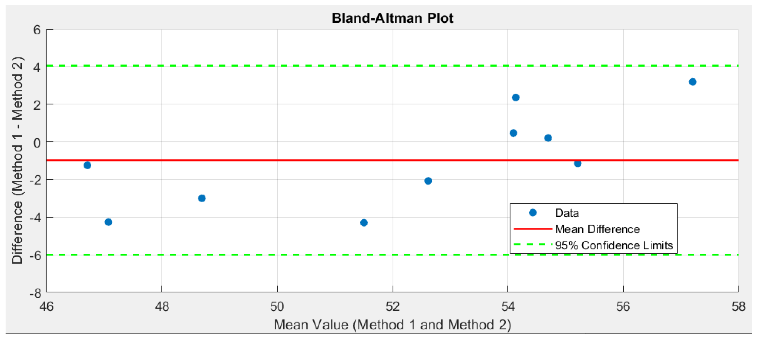
The Bland-Altman plot shown in Figure 10 illustrates the degree of agreement between the results of the two methods. The x-axis represents the average values of the two methods, while the y-axis shows the differences between them. The purpose of this plot is to identify systematic biases and evaluate the consistency between the methods.
The central line represents the mean difference between the methods, while the two parallel lines on either side indicate the 95% confidence limits, within which 95% of the differences are expected to fall. Data points outside these limits are considered anomalies or deviations. In this case, no such values are observed.
The correlation coefficient for the analyzed values of the two methods falls within the 95% confidence interval. The lower bound of the interval (0.53194) indicates a moderate relationship, while the upper bound (0.96893) reflects an exceptionally strong correlation. The narrow width of the interval signifies the stability and reliability of the calculated correlation.
These results clearly support the conclusion that a reliable and significant linear relationship exists between the analyzed variables. The accompanying graphs and analyses provide a clear and comprehensive visualization of the study’s findings. The proposed methodology in Method 1 ensures a thorough and transparent analysis, enabling an objective comparison of the methods used and their effectiveness.
6. Conclusions
This The comparative analysis of the two methodologies for assessing the risk of pedestrian-involved traffic accidents – the proportional risk distribution and the Random Forest algorithm – demonstrates their equal applicability for studying complex systems with multiple interrelated factors. Although the Random Forest algorithm exhibits higher accuracy and the ability to process heterogeneous data, the proportional dependence methodology offers a simplified and intuitive approach for evaluation. The two methodologies complement each other and can be effectively used for reliable risk assessment and forecasting in the context of traffic safety. The results support the thesis that the choice of methodology depends on the specifics of the study and the available data, with both approaches providing a solid foundation for making informed decisions.
Author Contributions
Conceptualization, H. U and P. M.; methodology, H.U and P. M.; software, S.D.; data curation, V.U. All authors participated equally in the research. All authors have read and agreed to the published version of the manuscript.
Funding
Please add The APC was founded by the Scientific and Research Sector of the Technical University of Sofia, Bulgaria.
Data Availability Statement
Not applicable.
Acknowledgments
This scientific publication is funded under the project “Improvement of Research Capacity and Quality for International Recognition and Sustainability of Sofia University of Technology” with contract number BG-RRP-2.004.0005, implemented within the framework of the National Research Infrastructure (NRI) at Sofia University of Technology by scientific group 3.4.14 “Development of a Cloud-Based Research Infrastructure Platform for Innovative Technologies in Road Safety.” We express our sincere gratitude for the support and assistance provided.
Conflicts of Interest
The authors declare no conflict of interest.
References
- Abdel-Aty, M.; Lee, J.; Yu, R. Analysis of pedestrian crashes using machine learning algorithms. Accident Analysis & Prevention 2019, 131, 285–293. [CrossRef]
- Stamov, G.; Stamova, I.; Simeonov, S.; Torlakov, I. On the Stability with Respect to H-Manifolds for Cohen–Grossberg-Type Bidirectional Associative Memory Neural Networks with Variable Impulsive Perturbations and Time-Varying Delays. Mathematics 2020, 8(3), 335. [CrossRef]
- Shahin Mirbakhsh, M.; Azizi, M. A Machine Learning Method for Improving the Safety of Pedestrians on Roadways. Journal of Industrial Safety Engineering 2024. https://journals.stmjournals.com/joise/article=2024/view=156953/.
- Theofilatos, A.; Yannis, G. A review of the effect of traffic and weather characteristics on road safety. Accident Analysis & Prevention 2014, 72, 244–256. [CrossRef]
- Peng, Y.; Abdel-Aty, M.; Shi, Q.; Yu, R. Assessing the impact of reduced visibility on traffic crash risk using microscopic data and surrogate safety measures. Transportation Research Part C: Emerging Technologies 2017, 74, 295–305. [CrossRef]
- Gospodinova, E.; Torlakov, I.; Metodieva, I. Model for Forecasting and Planning Solar Energy Production Using an Artificial Neural Network. In 2023 3rd International Conference on Electrical, Computer, Communications and Mechatronics Engineering (ICECCME); IEEE, 2023; pp. 1–6. [CrossRef]
- Mokhtarimousavi, S.; Anderson, J. C.; Azizinamini, A.; Hadi, M. Improved Support Vector Machine Models for Work Zone Crash Injury Severity Prediction and Analysis. Transportation Research Record 2019, 2673(11), 680–692. [CrossRef]
- Stamov, G.; Simeonov, S.; Torlakov, I.; Yaneva, M. Parallel Technique on Bidirectional Associative Memory Cohen-Grossberg Neural Network. In Recent Contributions to Bioinformatics and Biomedical Sciences and Engineering; Springer, 2023; pp. 16–20. [CrossRef]
- Gospodinova, E.; Torlakov, I. Information Processing with Stability Point Modeling in Cohen–Grossberg Neural Networks. Axioms 2023, 12(7), 612. [CrossRef]
- Breiman, L. Random forests. Machine Learning 2001, 45(1), 5–32. [CrossRef]
- Chen, X.; Zhang, Y.; Zhu, Z.; Wang, J. Real-time pedestrian detection and tracking for intelligent transportation systems using deep learning. Transportation Research Part C: Emerging Technologies 2020, 111, 62–78. [CrossRef]
- He, H.; Garcia, E. A. Learning from imbalanced data. IEEE Transactions on Knowledge and Data Engineering 2009, 21(9), 1263–1284. [CrossRef]
- Delen, S.; Sharda, R.; Bessonov, M. Identifying significant predictors of injury severity in traffic accidents using a series of artificial neural networks. Accident Analysis & Prevention 2006, 38(3), 434–444. [CrossRef]
- Alkheder, S.; Taamneh, M.; Taamneh, S. Severity prediction of traffic accident using an artificial neural network. Journal of Forecasting 2017, 36(1), 100–108. [CrossRef]
- Stamov, G.; Simeonov, S.; Torlakov, I. Visualization on Stability of Impulsive Cohen-Grossberg Neural Networks with Time-Varying Delays. In Contemporary Methods in Bioinformatics and Biomedicine and Their Applications; Springer, 2022; pp. 195–201. [CrossRef]
- Stamov, G.; Simeonov, S.; Torlakov, I. Software Analysis of Bidirectional Associative Memory (BAM) Cohen–Grossberg-Type Impulsive Neural Networks with Time-Varying Delays. In Proceedings of Seventh International Congress on Information and Communication Technology; Springer, 2022; pp. 371–378. [CrossRef]
- Gospodinova, E.; Torlakov, I.; Metodieva, I. Increasing the Productivity of an Electricity System Based on Energy Generated by Hydropower with the Help of Artificial Intelligence. In 2023 58th International Scientific Conference on Information, Communication and Energy Systems and Technologies (ICEST); IEEE, 2023; pp. 205–208. [CrossRef]
- Gospodinova, E.; Torlakov, I. Usage of High-Performance System in Impulsive Modelling of Hepatitis B Virus. In Lecture Notes in Networks and Systems; Springer, 2023; pp. 373–385. [CrossRef]
- Zhang, G.; Yau, K. K. W.; Chen, G. Risk factors associated with traffic violations and accident severity in China. Accident Analysis & Prevention 2016, 95, 503–511.
- Tang, J.; Liu, F.; Zou, Y.; Zhang, W.; Wang, Y. An improved fuzzy neural network for traffic speed prediction considering periodic characteristic. IEEE Transactions on Intelligent Transportation Systems 2017, 18(9), 2340–2350. [CrossRef]
Figure 1.
Diagram of the system: driver, vehicle, road, and environment.
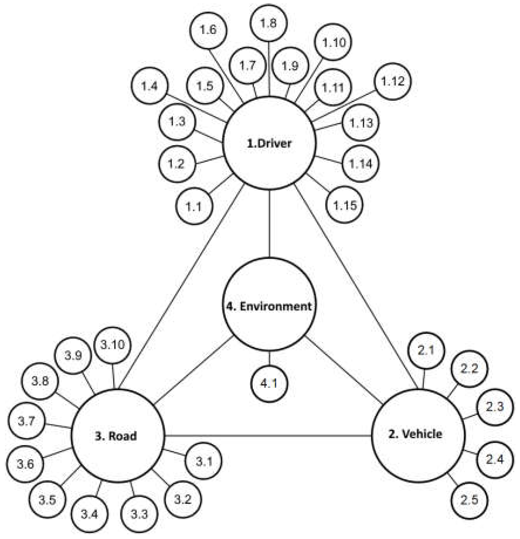
Figure 2.
Graph Depicting the Significance of Linguistic Variables.
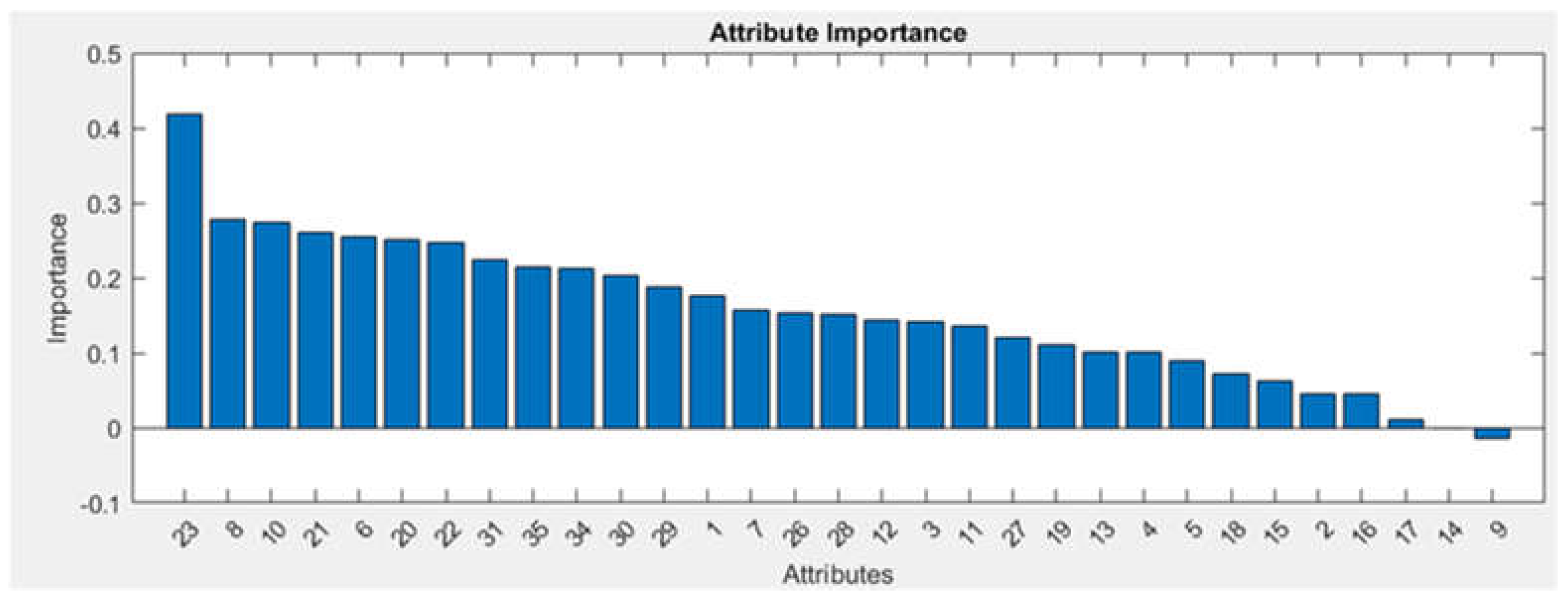
Figure 3.
Graph of Out-of-Bag Error Values.
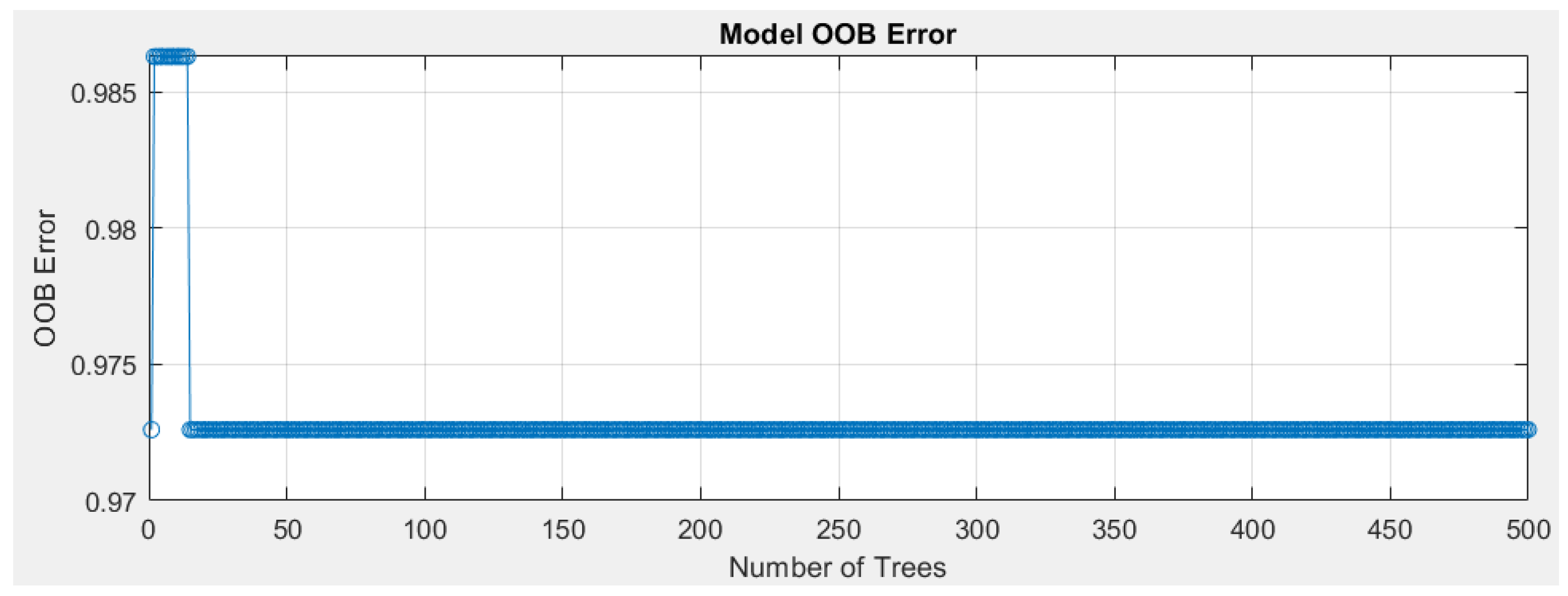
Figure 4.
Correlation Graph Between Variables.
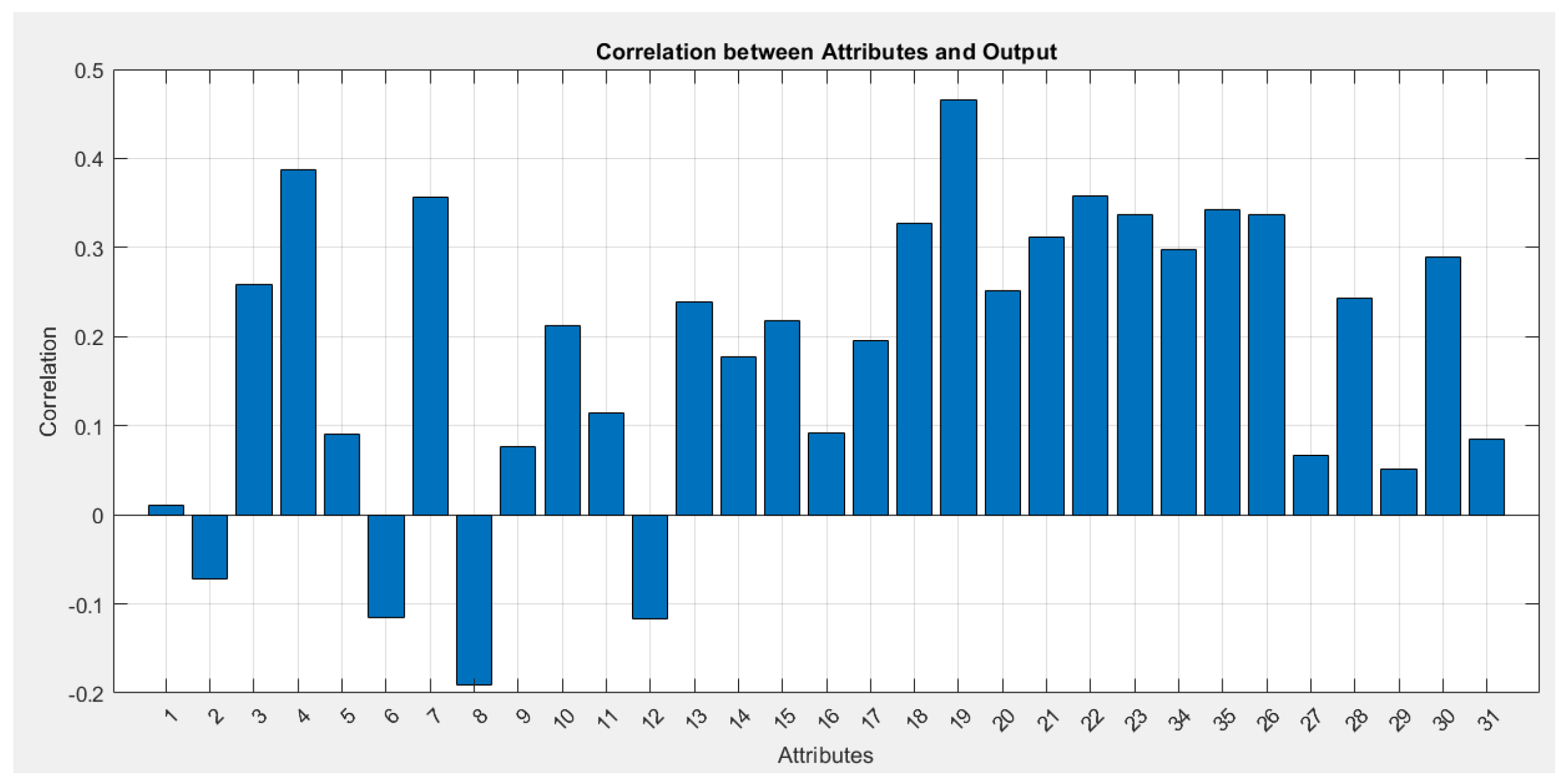
Figure 5.
Graph of the First Tree in the Model Structure.
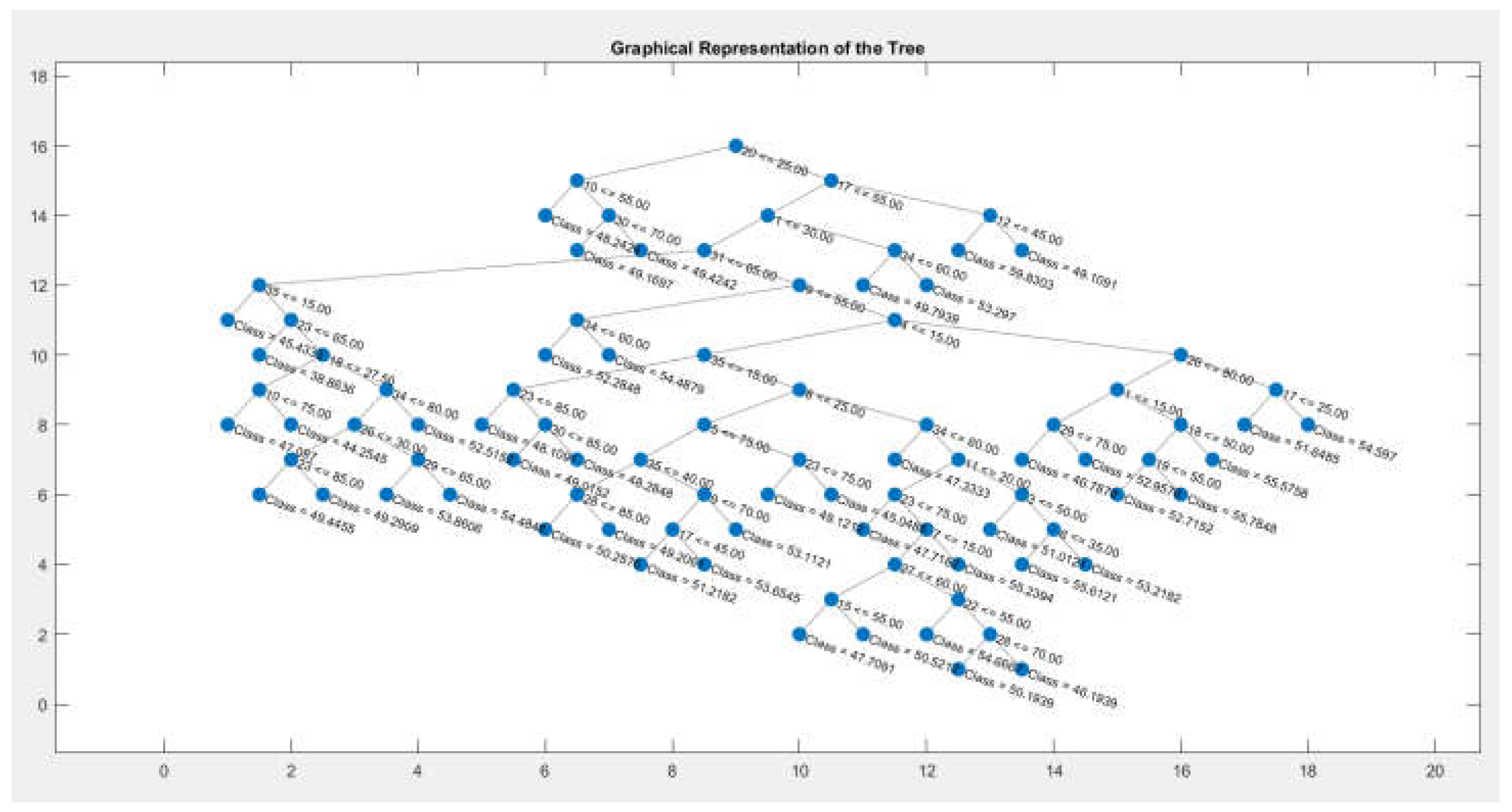
Figure 6.
Graph of the Second Tree in the Model Structure.
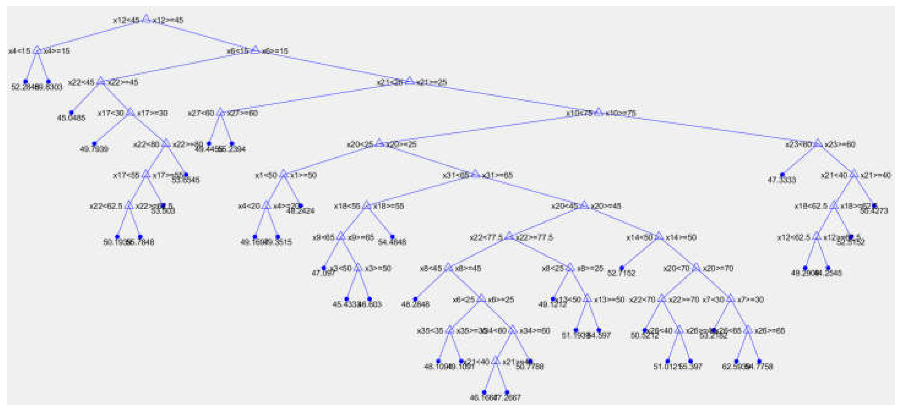
Figure 7.
Graphical dependencies of the risk assessment methods according to the output values.
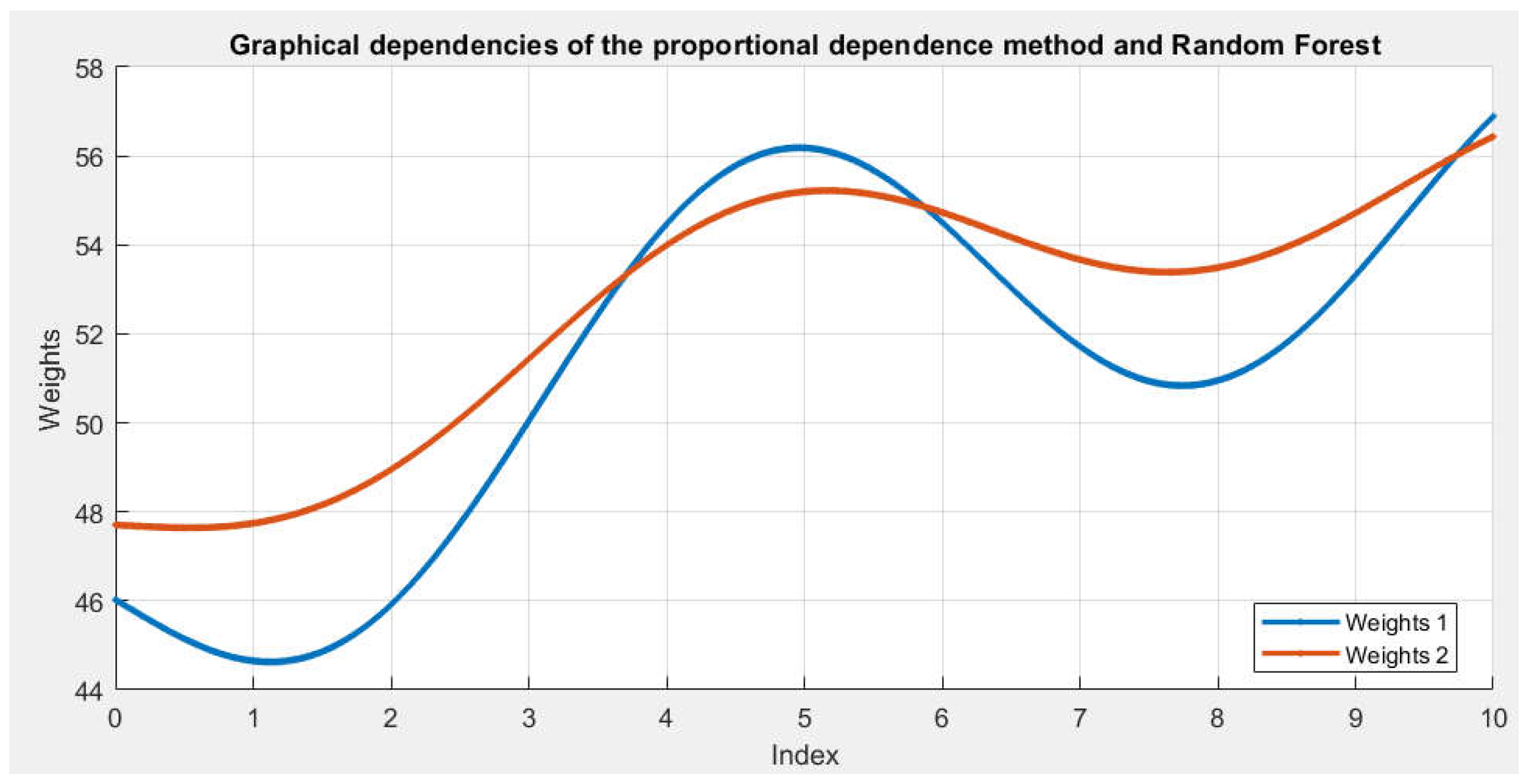
Figure 8.
Scatter plot and correlation coefficient.
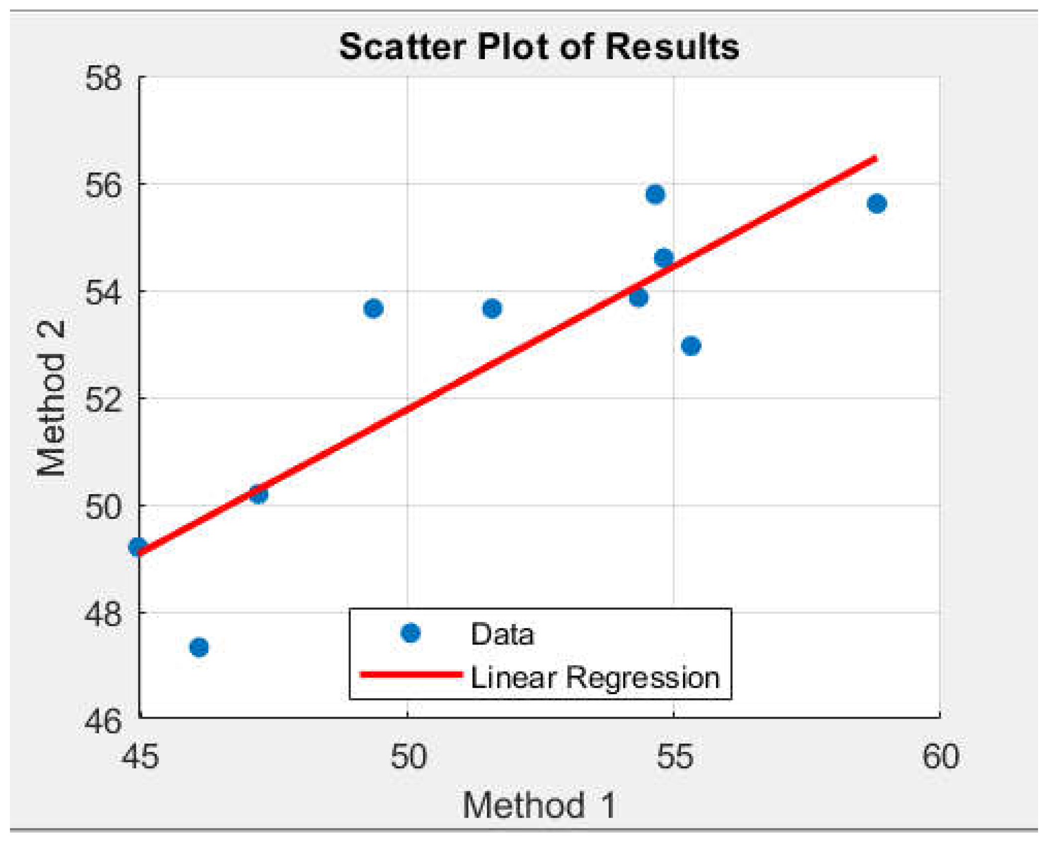
Figure 9.
Scatter plot and correlation coefficient.
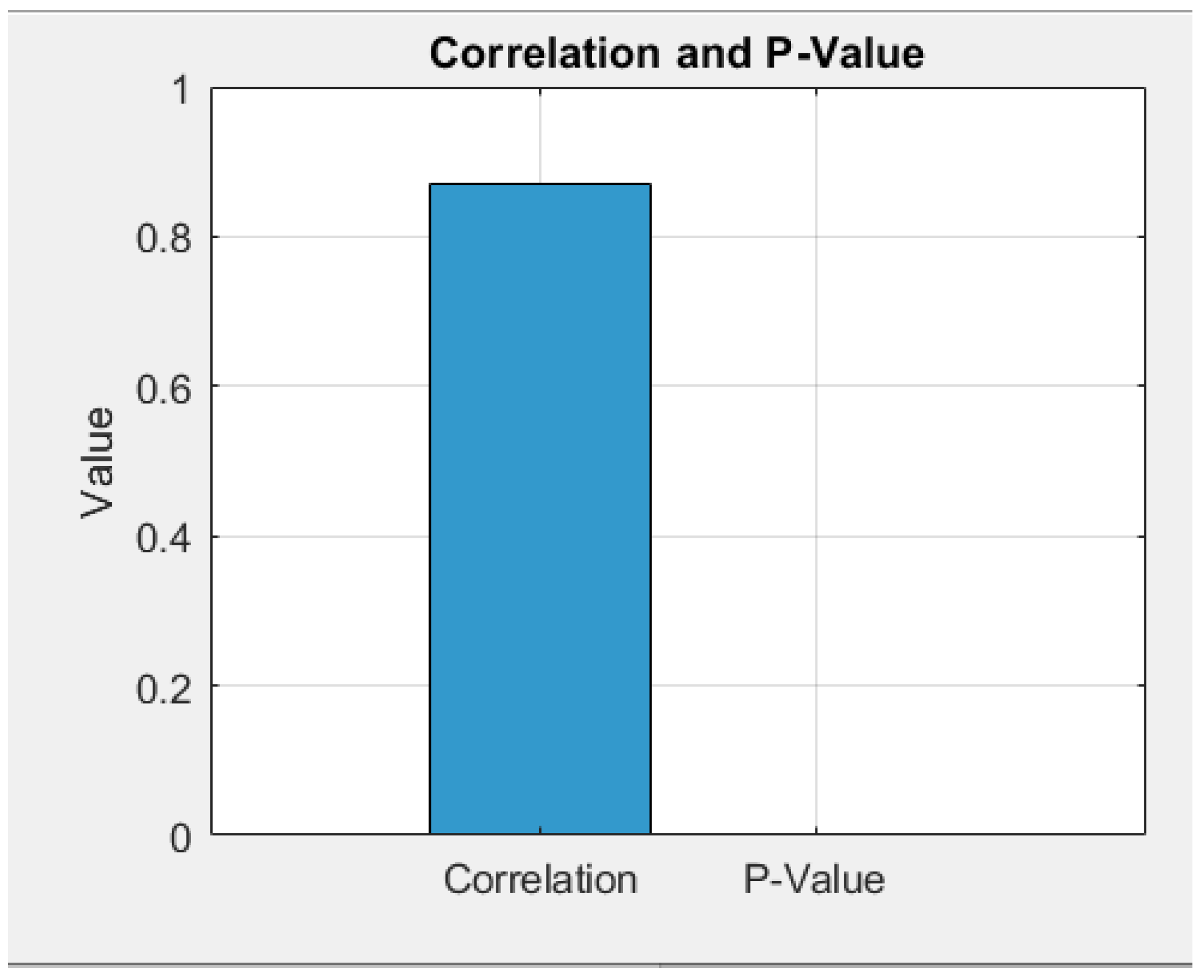
Figure 10.
Bland-Altman plot.
Disclaimer/Publisher’s Note: The statements, opinions and data contained in all publications are solely those of the individual author(s) and contributor(s) and not of MDPI and/or the editor(s). MDPI and/or the editor(s) disclaim responsibility for any injury to people or property resulting from any ideas, methods, instructions or products referred to in the content. |
© 2025 by the authors. Licensee MDPI, Basel, Switzerland. This article is an open access article distributed under the terms and conditions of the Creative Commons Attribution (CC BY) license (http://creativecommons.org/licenses/by/4.0/).
Copyright: This open access article is published under a Creative Commons CC BY 4.0 license, which permit the free download, distribution, and reuse, provided that the author and preprint are cited in any reuse.


