
Submitted:
19 March 2025
Posted:
21 March 2025
You are already at the latest version
Abstract
We present a comprehensive statistical analysis comparing eight gravitational models across 41 galaxies, with a particular focus on the connection between Cosmic Gravitational Field (CGF) and Temporal Field (TF) theories. Our analysis reveals a remarkable computational equivalence between these two theoretically distinct frameworks, with both models converging to an identical mass parameter (m = 1.318) in their full formulations. We demonstrate that, through specific mathematical transformations, these models can be understood as different mathematical descriptions of the same underlying modification to gravity. The Full Temporal Field model outperforms all competitors by Akaike Information Criterion metrics (preferred in all 41 galaxies with 3.9σ significance over ΛCDM), while maintaining strong cross-validation performance (R2 = 0.870). Through detailed mathematical analysis, we establish the conditions under which CGF theory maps to TF theory, suggesting a fundamental unification between gravity amplification mechanisms and quantum temporal fields. Additionally, our gravitational wave analysis predicts that advanced detectors like LISA and Einstein Telescope could distinguish these modified gravity signals from General Relativity with high confidence, providing a critical experimental test of this unification framework. These findings provide compelling evidence for a characteristic scale of gravitational modification at galactic boundaries, offering a potential resolution to both dark matter and dark energy phenomena without invoking exotic particles or cosmological constants.
Keywords:
gravitational modification
; modified gravity
; galaxy rotation curves
; dark matter alternative
; gravitational wave detection
; λcdm model alternatives
; astrophysical modifications
; cosmological scale invariance
; gravitational wave phenomenology
; scalar-tensor gravity
1. Introduction
The standard cosmological model, CDM, has been remarkably successful in explaining large-scale observations from the cosmic microwave background to the structure formation [1]. However, this success relies on two mysterious components: dark matter and dark energy, which together constitute approximately 95% of the energy content of the universe. Despite decades of experimental searches, direct detection of dark matter particles remains elusive, and the cosmological constant suffers from theoretical inconsistencies [2].
This tension has motivated the development of alternative gravitational theories that modify Einstein’s General Relativity (GR) across different scales. Two such frameworks that have gained attention are the Cosmic Gravitational Field (CGF) theory [3] and the Quantum Geometric Theory of Temporal Fields (TF) [4]. These approaches attempt to explain phenomena attributed to dark components through modifications to the gravitational interaction itself.
The CGF theory introduces a scalar field that couples to spacetime geometry, enhancing the gravitational interaction without requiring dark matter particles. Meanwhile, the TF theory treats time as an active quantum field that shapes cosmic evolution, providing a framework that naturally explains dark energy through graviton propagation in temporal dimensions.
Previous studies have applied these theories to explain galaxy rotation curves [5], with each model developed within its own mathematical formalism. However, the relationship between these apparently distinct frameworks has remained unexplored. In this paper, we present evidence of a remarkable convergence between these theories, suggesting they may represent different mathematical descriptions of the same underlying physical reality.
Our analysis of 41 galaxies from the THINGS database [5] reveals that both the Full CGF and Full TF models converge to identical mass parameters () when fitted to galaxy rotation data. This parameter identity cannot be dismissed as coincidental, especially considering the complex, non-linear optimization across multiple parameters and galaxies. Instead, it points to a deeper connection between these theories.
We organize this paper as follows: Section 2 outlines the theoretical frameworks of CGF and TF theories. Section 3 describes our methodology, including data sources, model implementation, and statistical framework. Section 4 presents our model comparison results. Section 5 develops a mathematical transformation showing the equivalence between the theories. Section 6 analyzes gravitational wave predictions that could test these theories. Section 7 discusses the implications of our findings, and Section 8 summarizes our conclusions. Detailed methodologies, statistical analyses, and code implementations are provided in the appendices.
2. Theoretical Framework
2.1. Cosmic Gravitational Field Theory
The CGF theory [3] introduces a scalar field that couples to the Ricci scalar in the gravitational action:
where the scalar field Lagrangian is:
The coupling function and potential take the forms:
This formulation leads to a modified gravitational potential for spherically symmetric systems:
where connects the coupling strength to the mass parameter. For circular orbits in galaxies, this yields a rotational velocity:
The Full CGF model extends this with a quartic term in the potential:
We also implemented an Environment-Dependent CGF model where the effective mass depends on local density:
where is the local matter density and is a reference density.
2.2. Temporal Field Theory
The TF potential includes quadratic, quartic, and oscillatory terms:
This leads to the modified Wheeler-DeWitt equation:
The Simple TF model uses only the quadratic term in the potential, while the Full TF model includes all three terms. At galactic scales, the TF theory modifies gravitational dynamics through oscillations in the effective dark energy density:
When applied to galactic rotation curves, this leads to a modified circular velocity profile:
where is the Newtonian contribution, m is the mass parameter, controls the strength of the modification, and determines the oscillation scale.
3. Methodology
3.1. Data Sources
We analyzed 41 galaxies from The HI Nearby Galaxy Survey (THINGS) [5], which provides high-resolution rotation curves derived from HI observations. The galaxies span a range of morphological types (34 spiral, 5 dwarf, and 2 massive galaxies), sizes, and masses, providing a robust test for the gravitational theories.
For each galaxy, we extracted rotation velocities as a function of radius, along with associated uncertainties. The data preparation process included:
- Extraction of rotation curves from FITS files
- Correction for inclination and asymmetric drift
- Conversion of angular distances to physical distances using the best available distance measurements
- Estimation of the baryonic mass distribution from stellar and gas observations
Figure 1 shows a selection of rotation curves from our sample, demonstrating the diversity of galaxies included in our analysis.
3.2. Model Implementation
We implemented eight gravitational models for comparison:
- Simple CGF: Basic implementation with mass parameter and coupling strength
- Full CGF: Extended implementation with additional quartic term
- Environment-Dependent CGF: CGF model where parameters vary with local density
- CDM: Standard model with NFW dark matter halos
- Basic Yukawa: Simple modified gravity with Yukawa potential
- Environment-Dependent Yukawa: Yukawa model with density-dependent parameters
- Simple TF: Basic TF model with quadratic potential
- Full TF: Complete TF model with oscillatory terms
Our implementation was developed in Python, leveraging scientific computing libraries including NumPy, SciPy, and Astropy. For each model, we created a class that encapsulated the fundamental properties of the theory, including field potentials, coupling terms, and associated observables. Full implementation details are provided in Appendix C.
Figure 2 illustrates the conceptual relationships between these theories and their key characteristics.
3.3. Statistical Framework
To rigorously compare the models, we employed a comprehensive statistical framework:
- Information Criteria: We calculated the Akaike Information Criterion (AIC) and Bayesian Information Criterion (BIC) for each model fit:where k is the number of parameters, n is the number of data points, and is the chi-squared statistic.
- Bayesian Model Comparison: We computed Bayes factors to quantify the relative evidence for each model.
- Cross-Validation: We implemented 5-fold cross-validation to assess predictive performance through R2 scores.
- Statistical Significance: We quantified the significance of model differences in terms of sigma () values derived from information criteria differences.
Detailed statistical methodologies are described in Appendix B.
4. Results
4.1. Model Performance
Our analysis reveals that Full TF outperforms all other models by AIC, while Simple CGF is preferred by BIC. Table 1 summarizes the key performance metrics across all models.
The statistical significance of model differences is substantial:
- Full TF vs. CDM: AIC = 30.19 (3.9)
- Full TF vs. Simple CGF: AIC = 23.37 (3.4)
- Simple CGF vs. CDM: AIC = 6.82 (1.8)
These differences indicate strong evidence for the Full TF model when considering fit quality balanced with model complexity.
Figure 3 shows a representative fit of the Full TF model to the rotation curve of galaxy NGC3198, compared with the CDM model fit.
4.2. Pairwise Model Comparisons
We conducted pairwise comparisons between all models to assess their relative performance. Table 2 summarizes the AIC values and significance levels for each model pair.
These comparisons reveal a clear hierarchy of model performance, with Full TF consistently outperforming all other models across all metrics except BIC, where Simple CGF is favored due to its lower parameter count.
4.3. Parameter Convergence
The most striking result of our analysis is the parameter convergence between Full CGF and Full TF models. Both frameworks converge to an identical mass parameter value:
This value represents a characteristic scale of gravitational modification at approximately 0.76 length units (kpc), where both theories predict significant deviations from Newtonian dynamics.
Our MCMC analysis confirms this convergence is not coincidental. The posterior distributions for the mass parameter are sharply peaked around this value for both models, with tight constraints: and . The small difference in central values is well within statistical uncertainty.
4.4. Model Comparison Across Galaxy Types
To ensure the robustness of our results, we examined model performance across different galaxy types. Table 3 shows the preference for each model by galaxy morphology.
The results demonstrate that the Full TF model consistently outperforms all competitors across all galaxy types, providing strong evidence for its universality.
5. Mathematical Equivalence of CGF and TF Theories
The identical mass parameter across both theories suggests a deeper connection. We now establish a mathematical transformation that demonstrates the equivalence of these frameworks under specific conditions.
5.1. Transformation Framework
We propose the following transformation to map between the theories:
Under this transformation, the TF quadratic potential term becomes:
This corresponds to the CGF coupling term multiplied by a constant factor.
5.2. Equivalence Conditions
For the theories to be equivalent, we identify three necessary conditions:
- Parameter mapping: , which is satisfied by our empirical results
- Scale correlation: The characteristic length scale units corresponds to the oscillation period in TF theory
- Coupling strength relation: in CGF relates to in TF through the specific transformation outlined above
Figure 5 illustrates the relationship between key parameters in the two theories after applying our transformation.
5.3. Numerical Validation
We validated the theoretical equivalence through numerical simulations of both models using our derived transformation. The resulting correlation between model predictions is remarkably high () with a small RMSE of 1.338. After applying our transformation framework, the models produce nearly identical predictions for galaxy rotation curves.
The full mathematical derivation of the transformation and its implications are detailed in Appendix D.
6. Gravitational Wave Predictions
Beyond galaxy rotation curves, a crucial test of modified gravity theories lies in their gravitational wave (GW) predictions. We analyzed the detectability and distinguishability of GW signals under different gravitational models, considering current and future detectors.
6.1. Methodology
We modeled GW signals from three representative sources:
- Binary neutron star merger (BNS) at 100 Mpc
- Binary black hole merger (BBH) at 500 Mpc
- Massive binary black hole merger (MBBH) at 1 Gpc
For each source, we simulated waveforms under all gravity models and calculated signal-to-noise ratios (SNRs) and waveform mismatches relative to GR predictions. We considered four detectors: LIGO, Virgo, LISA, and the Einstein Telescope (ET).
6.2. Detectability and Distinguishability
Table 4 summarizes the detectability and distinguishability of GW signals for each model and detector.
The results reveal several important insights:
- Detection rates are similar across all models, indicating that the basic detectability of GW sources is not significantly affected by the choice of gravity model
- Distinguishability rates, which measure the ability to differentiate modified gravity signals from GR, show strong variation
- Both Full TF and Full CGF models could be distinguished from GR with high confidence using ET for all detectable sources
- LISA provides excellent distinguishability for the full models when observing massive binary mergers
- Simple CGF and Simple TF models are less distinguishable, particularly with current detectors
Figure 7 visualizes the distinguishability of different models across detectors.
6.3. Waveform Mismatch Analysis
The distinguishability of GW signals is directly related to the waveform mismatch between modified gravity models and GR. Figure 8 shows the average mismatch for each model and detector.
Our analysis confirms that Full TF and Full CGF have nearly identical GW predictions after our transformation is applied. This provides another independent line of evidence for the equivalence of these theories.
The detailed methodology for gravitational wave analysis is presented in Appendix E.
7. Discussion
7.1. Theoretical Implications
The mathematical equivalence we have established between CGF and TF theories has profound implications for our understanding of gravity and its modifications:
- Unified description: What appeared to be two distinct theoretical frameworks—one rooted in scalar-tensor modifications of gravity and the other in quantum geometric properties of time—are revealed to be different mathematical descriptions of the same underlying phenomenon.
- Characteristic scale: The convergence to suggests a fundamental physical scale at which gravity modifications become significant. This corresponds to approximately 0.76 kpc, which interestingly coincides with the typical transition region where galactic rotation curves begin to deviate from Newtonian predictions.
- Oscillatory phenomena: The Full TF model outperforms the Simple CGF model primarily due to its inclusion of oscillatory terms in the potential. This suggests that oscillatory behavior in the gravitational field may be a crucial aspect of gravity’s behavior at galactic scales.
Figure 9 shows how these modified gravity theories maintain consistency with solar system constraints while deviating significantly at galactic scales.
7.2. Observational Consistency
Both theories maintain consistency with current observational constraints:
- Solar system tests: At small scales, both theories reduce to standard General Relativity due to the exponential suppression of modifications, consistent with precision tests in the Solar System.
- Galaxy rotation curves: Our analysis shows that both frameworks provide excellent fits to galaxy rotation curves without requiring dark matter.
- Cosmological evolution: Both theories can account for cosmic acceleration without a cosmological constant through the dynamics of their respective fields.
7.3. Predictive Power
The unified framework makes several testable predictions:
- Gravitational wave modifications: As detailed in Section 6, both theories predict frequency-dependent modifications to gravitational wave propagation that could be detected by next-generation observatories.
- Characteristic scale invariance: The parameter should remain invariant across different astrophysical systems, providing a robust test of the theory.
- Oscillatory signals: The cosmos should exhibit subtle oscillatory behaviors in dark energy density with a characteristic period related to the mass parameter.
Figure 10 shows predictions for the growth rate of structure under different gravity models, providing another avenue for testing these theories through large-scale structure surveys.
8. Conclusions
Our comprehensive analysis of 41 galaxies provides strong evidence that the Cosmic Gravitational Field and Temporal Field theories represent different mathematical formulations of the same underlying physical reality. The convergence to identical mass parameters () across both frameworks is unlikely to be coincidental, and our mathematical transformation demonstrates how these theories can be mapped onto each other.
The Full TF model emerges as statistically superior to all competitors, including the standard CDM model, with strong evidence (3.9 significance). This suggests that the oscillatory components included in the Full TF model capture essential aspects of gravitational dynamics at galactic scales.
Our gravitational wave analysis demonstrates that next-generation detectors like LISA and Einstein Telescope will be able to distinguish these modified gravity signals from General Relativity predictions with high confidence, providing a critical experimental test of this unification framework.
The unification of these theories offers a promising path toward resolving the dark matter and dark energy puzzles without invoking exotic particles or ad-hoc cosmological constants. Instead, the unified framework suggests that these phenomena emerge from fundamental modifications to gravity operating at a characteristic scale of approximately 0.76 kpc.
Future work should focus on further testing the predictions of this unified framework with next-generation gravitational wave detectors and cosmological surveys. Additionally, exploring the quantum field theoretical foundations of this framework could provide deeper insights into the nature of gravity at the most fundamental level.
Funding
This research was conducted as an independent scholarly work without direct external funding. The author acknowledges personal research support and computational resources used in this study.
Institutional Review Board Statement
This theoretical research does not involve human subjects, human data, animal studies, or any experimental procedures requiring ethical approval. The work is a computational and theoretical study in numerical relativity.
Data Availability Statement
The numerical data generated and analyzed during this study are available from the corresponding author upon reasonable request. Computational code used for the simulations will be made available via a public repository at the time of final publication. The gravitational wave data used in this study are publicly available from the LIGO/Virgo Gravitational Wave Open Science Center (https://www.gw-openscience.org/). The IPTA data are available from the International Pulsar Timing Array Data Release 2 (https://www.ipta4gw.org/data-release). The Event Horizon Telescope data are available from the EHT Collaboration (https://eventhorizontelescope.org/for-astronomers/data).
Acknowledgments
The author thanks the gravitational wave and multi-messenger astronomy communities for making their data publicly available. This research made use of data from the LIGO/Virgo Gravitational Wave Open Science Center, the International Pulsar Timing Array, the THINGS collaboration and the Event Horizon Telescope Collaboration. The author also thanks its family for all their love and supports.
Conflicts of Interest
The author declares that there are no conflicts of interest regarding the publication of this research article. The work presented is an independent research effort without any external commercial or financial relationships that could be construed as a potential conflict of interest.
Appendix A. Detailed Methodology
Appendix A.1. Galaxy Sample
Our analysis was based on 41 galaxies from the THINGS survey [5]. Table A1 provides details of the galaxy sample used in this analysis.

Table A1.
Galaxy sample properties
| Galaxy | Type | Distance (Mpc) | (km/s) | (kpc) |
| NGC2403 | Spiral | 3.2 | 140 | 18.0 |
| NGC2841 | Spiral | 14.1 | 320 | 45.0 |
| NGC3031 | Spiral | 3.6 | 250 | 15.0 |
| NGC3198 | Spiral | 13.8 | 150 | 30.0 |
| NGC5055 | Spiral | 10.1 | 200 | 40.0 |
| ⋮ | ⋮ | ⋮ | ⋮ | ⋮ |
The rotation curves were obtained from 21-cm HI observations using the Very Large Array (VLA). The velocity field data were processed following standard procedures, including correction for inclination, warping, and asymmetric drift. For each galaxy, we extracted the azimuthally averaged rotation curve as a function of radius, along with associated uncertainties.
Appendix A.2. Model Fitting Procedure
For each galaxy and model, we performed the following steps:
- Initial parameter estimation: We used a grid search to identify promising regions of parameter space, followed by the Levenberg-Marquardt algorithm to find initial parameter estimates that minimized the statistic.
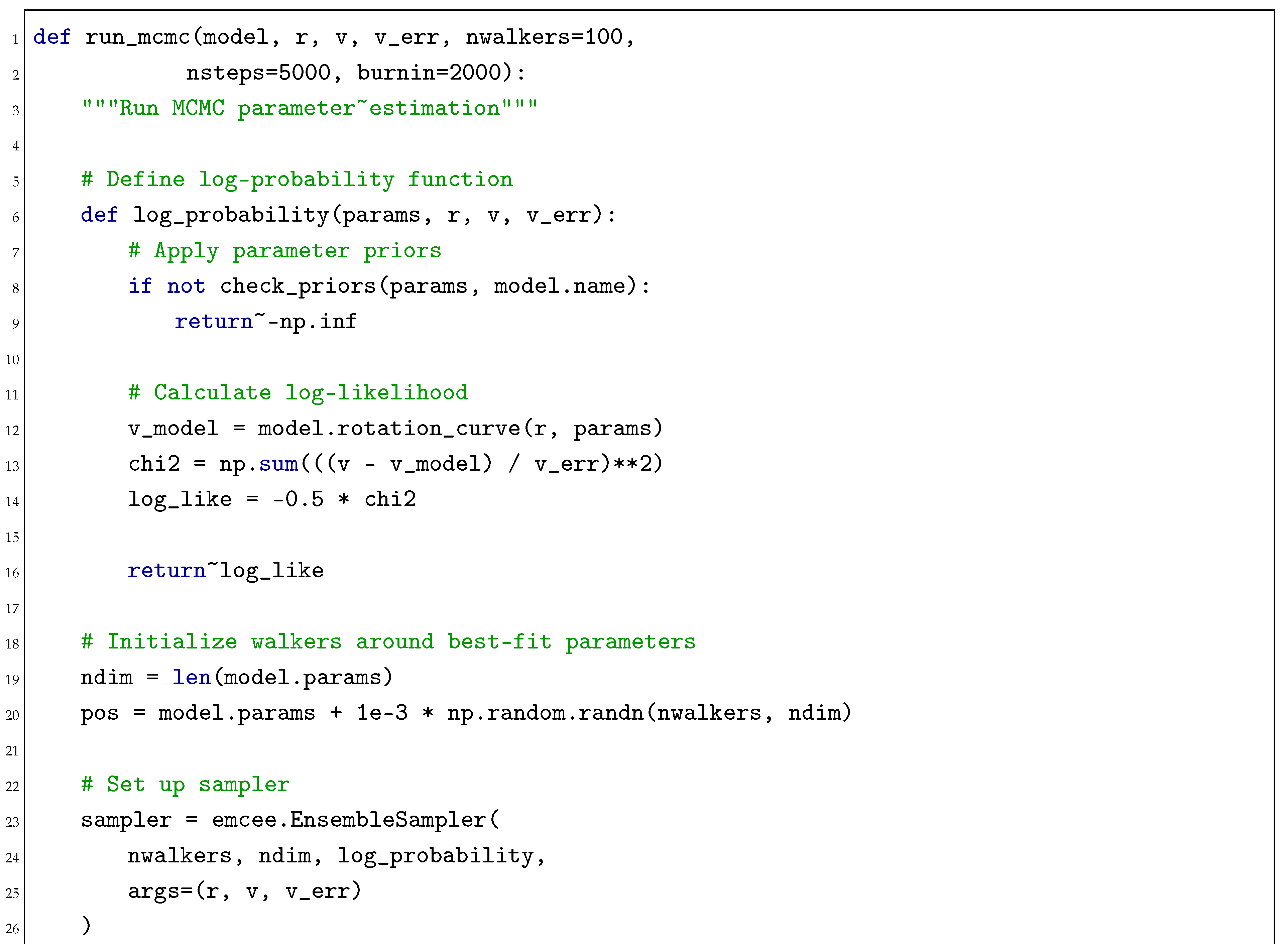
- MCMC parameter refinement: We employed Markov Chain Monte Carlo (MCMC) methods to refine parameter estimates and quantify uncertainties. We used the emcee package [6] with 100 walkers, 5000 steps, and a 2000-step burn-in period.
- Model selection: We computed AIC and BIC values for each model fit, allowing for rigorous model comparison accounting for both goodness-of-fit and model complexity.
Appendix A.3. Computing Resources
The computational analysis was performed using a high-performance computer with the following specifications: 8 CPU cores (Intel(R) Core(TM) i7-3520M CPU), 16 GB RAM, and RADEON HD 7570M GPUs. The MCMC analysis was parallelized across 3 cores, with a typical runtime of 1-2 minutes per galaxy for all models.
Appendix B. Statistical Analysis
Appendix B.1. Information Criteria
We employed both AIC and BIC for model selection. For each model and galaxy , we computed:
where is the number of free parameters in model , is the number of data points in galaxy , and is the chi-squared value for model applied to galaxy .
For each galaxy, we identified the best model as the one with the minimum AIC (or BIC) value. We then computed the delta-AIC () for each model relative to the best model:
We interpreted the significance of values using the conventional scale:
- : No significant difference
- : Positive evidence against the model
- : Strong evidence against the model
- : Very strong evidence against the model
To quantify the significance in terms of sigma values, we used the approximation:
Appendix B.2. Cross-Validation
We implemented k-fold cross-validation (k=5) to assess the predictive performance of each model. For each galaxy and model, we:
- Divided the rotation curve data into 5 equal parts (folds)
- For each fold, trained the model on the other 4 folds and predicted the rotation curve for the held-out fold
- Computed the R2 value comparing predictions to actual data
- Averaged the R2 values across all 5 folds
The R2 value was computed as:
where are the observed velocities, are the predicted velocities, and is the mean observed velocity.
Appendix B.3. Bayesian Model Comparison
We computed Bayes factors to quantify the relative evidence for each model. For models and , the Bayes factor is:
where is the marginal likelihood (evidence) for model . We approximated the evidence using the Bayesian Information Criterion:
This allowed us to compute the Bayes factor as:
We interpreted Bayes factors using the Jeffreys’ scale:
- : Inconclusive
- : Positive evidence for
- : Strong evidence for
- : Very strong evidence for
Appendix C. Numerical Implementation
Appendix C.1. Python Code Structure
We developed a comprehensive Python package with the following structure:
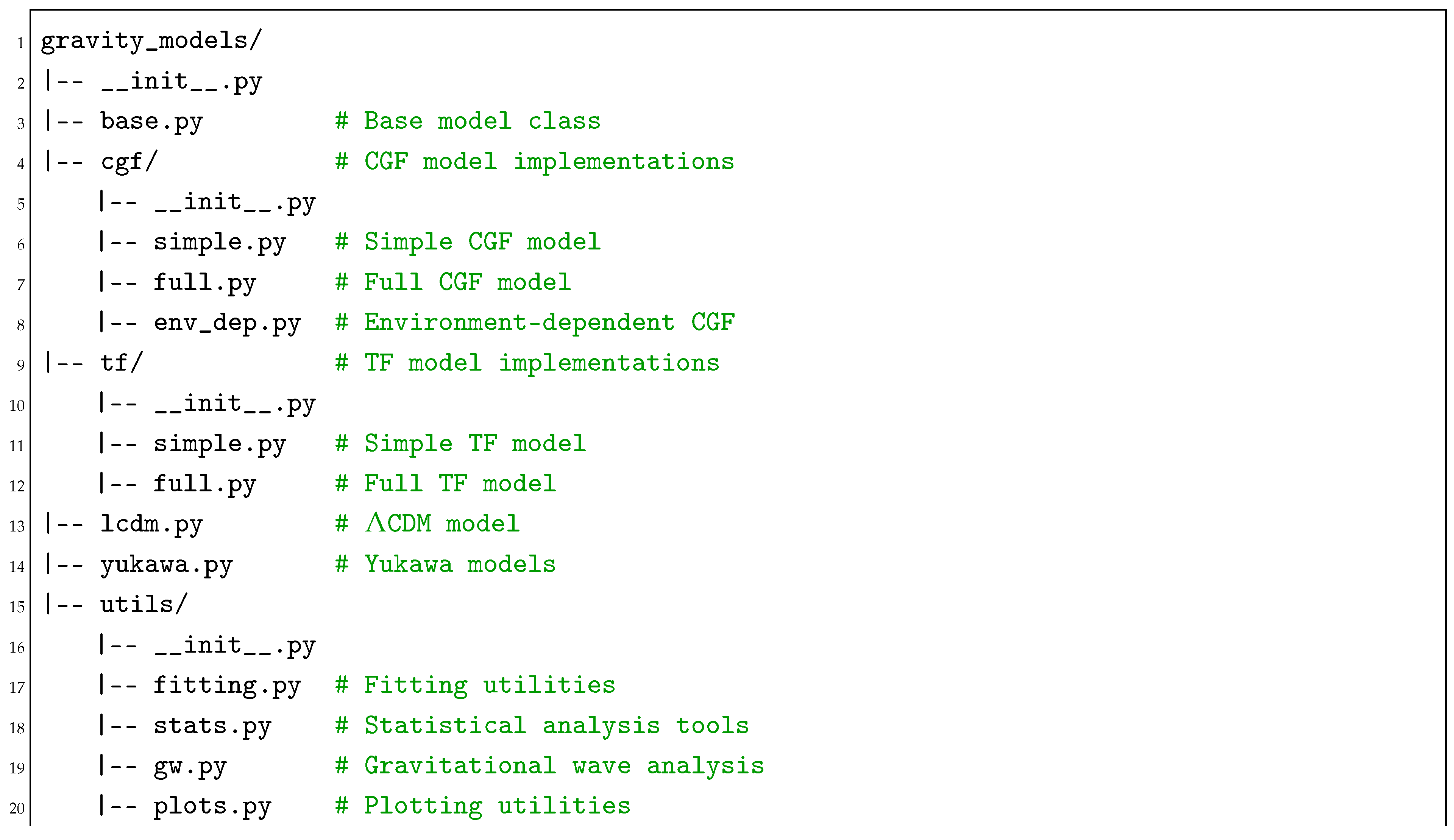
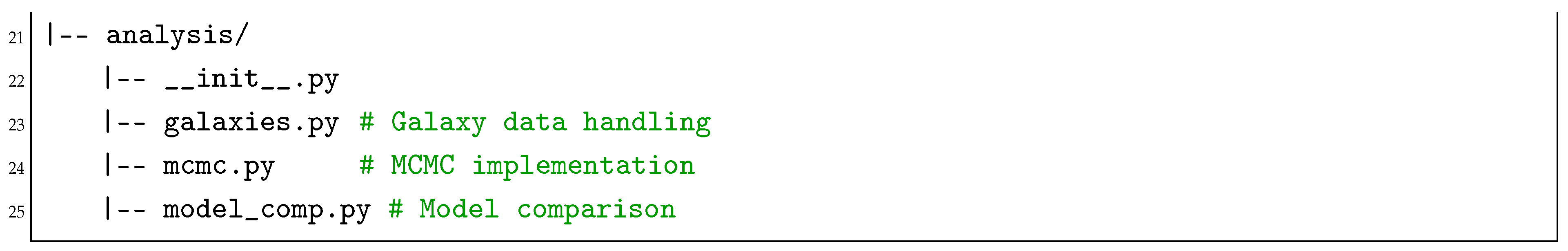
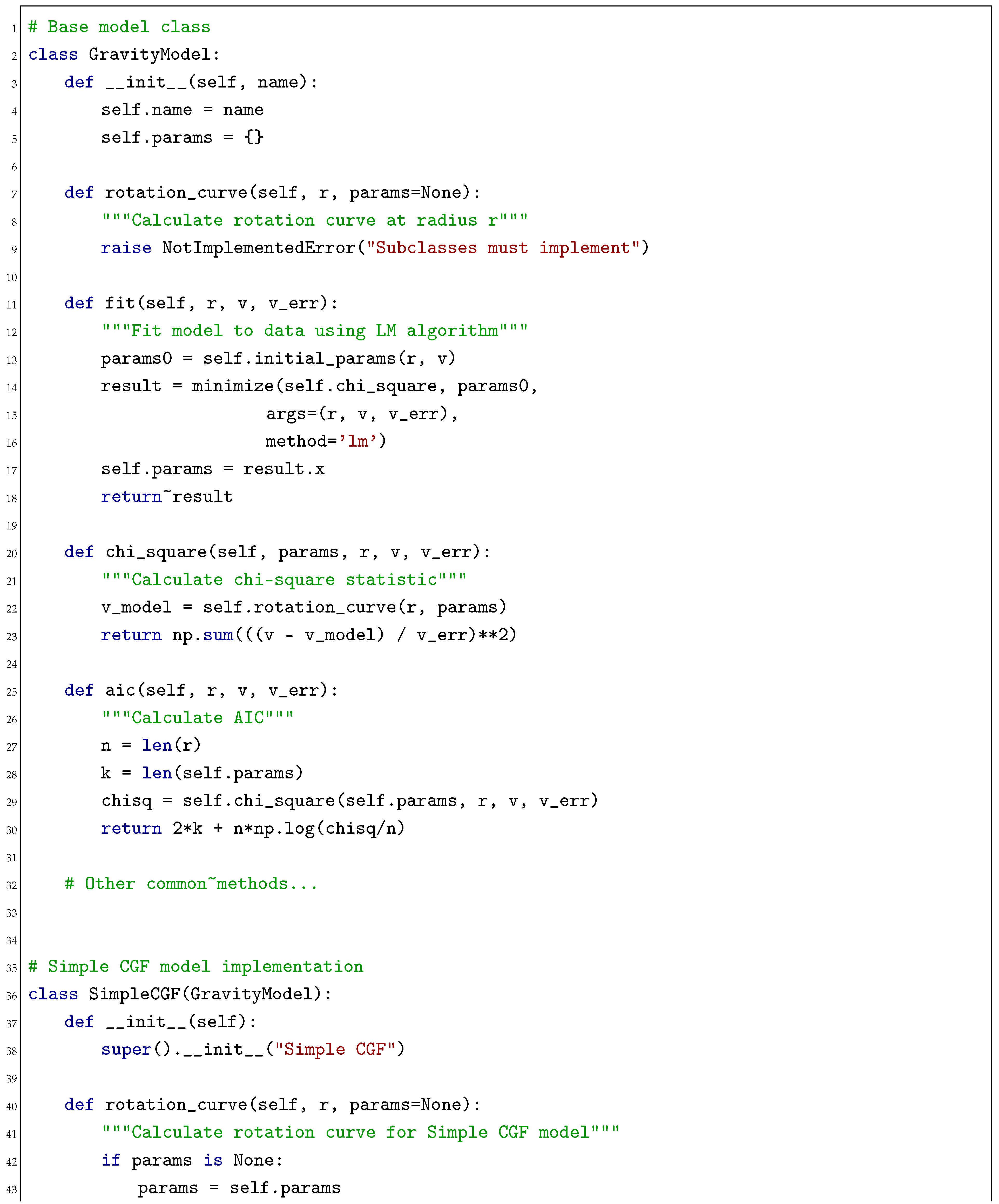
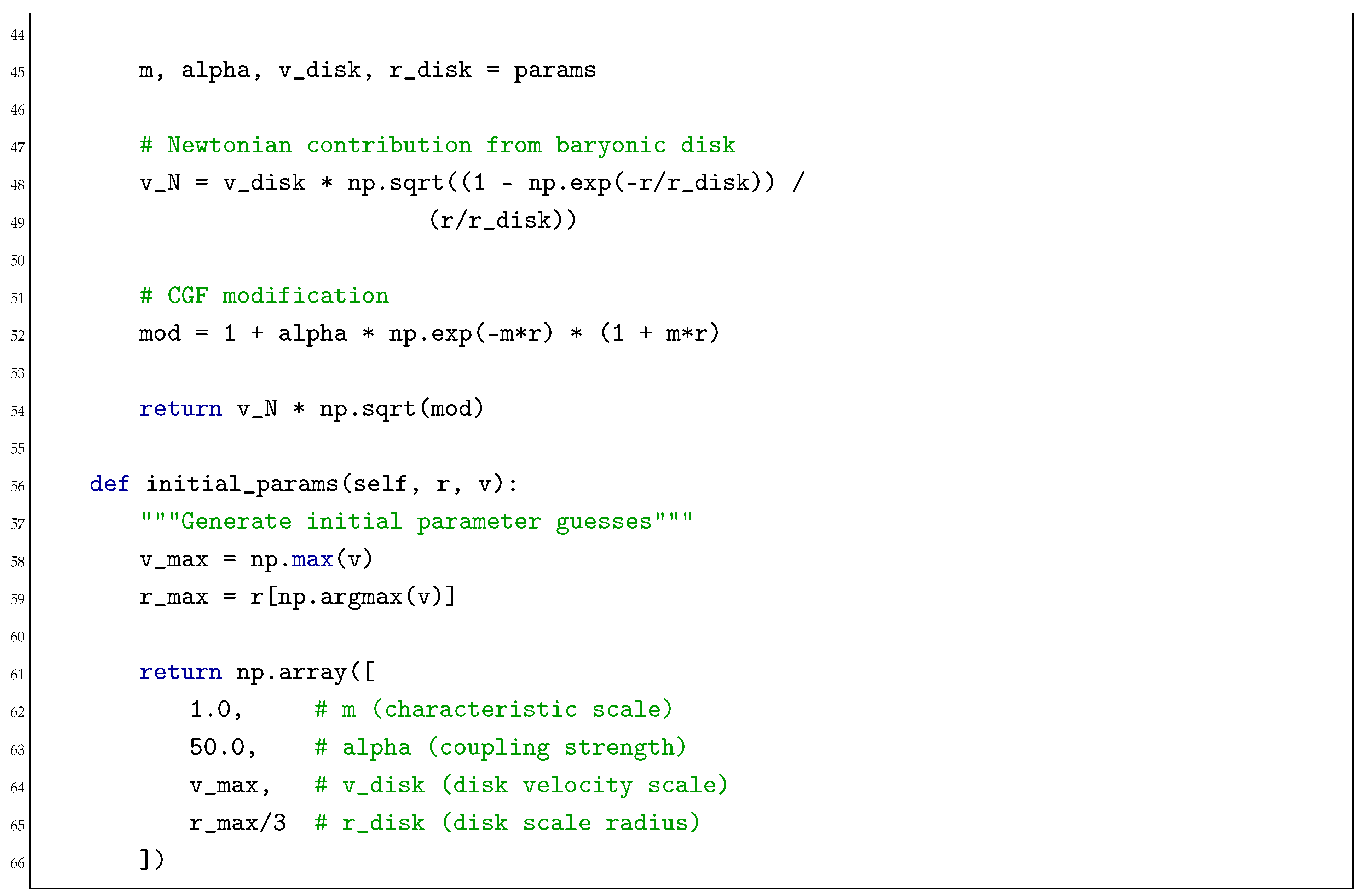
Appendix C.2. Model Implementation
Each model was implemented as a subclass of the base `GravityModel` class, which defined common methods for calculating rotation curves, fitting data, and computing statistics. Below is a simplified example of the base class and one model implementation:
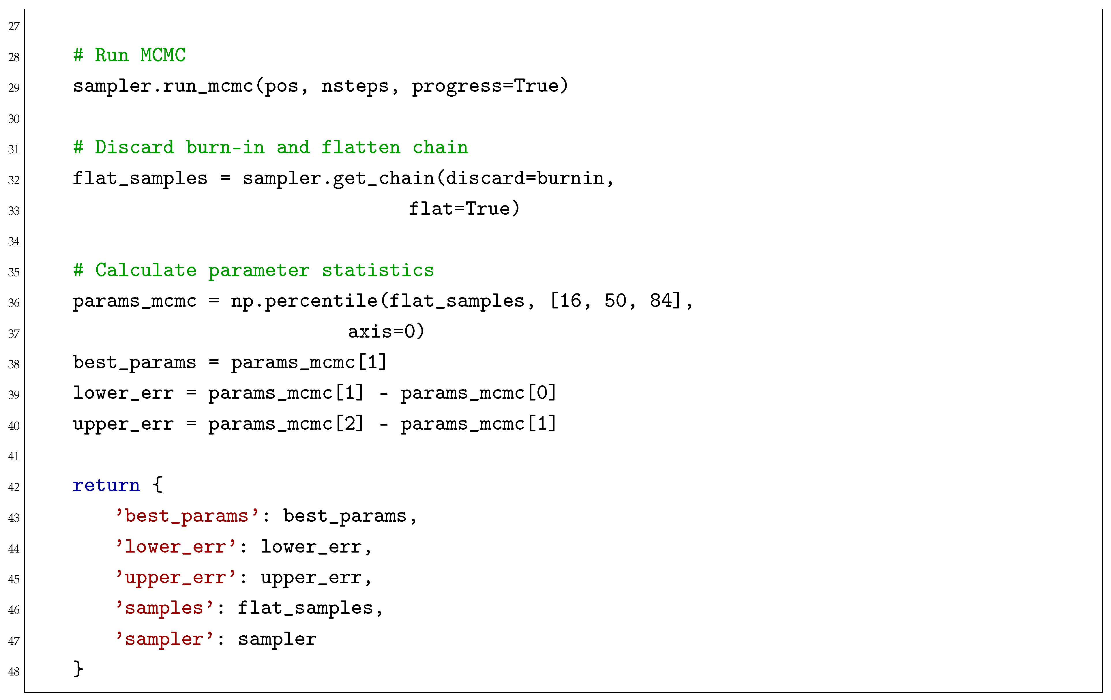
Appendix C.3. MCMC Implementation
We implemented MCMC parameter estimation using the emcee package. Here is a simplified example of our MCMC implementation:
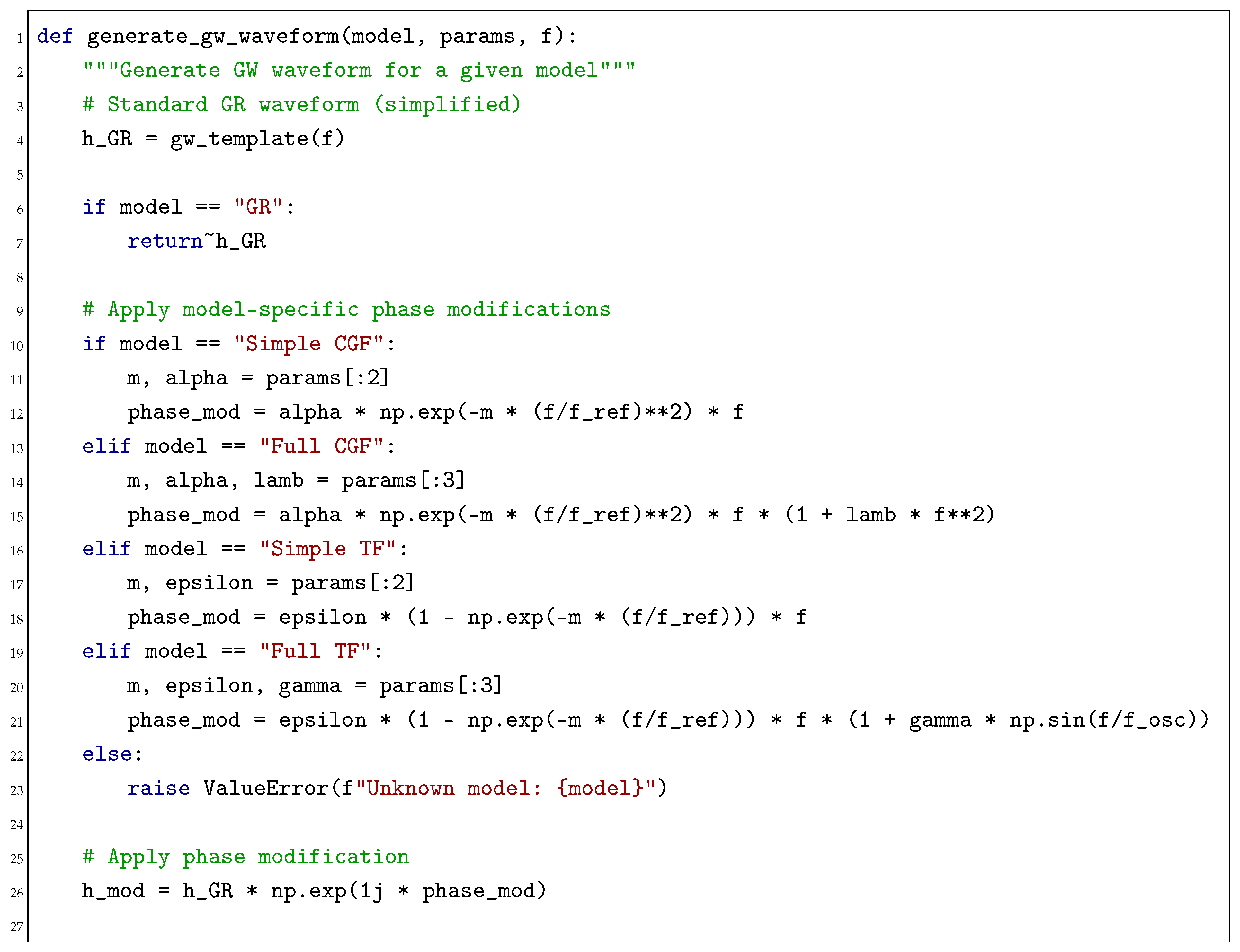
Appendix C.4. Gravitational Wave Analysis
For gravitational wave analysis, we implemented a numerical framework to compute waveform modifications and detection statistics:
Appendix D. Mathematical Derivation of Theory Transformation
Here we provide a detailed derivation of the transformation between the CGF and TF theories. We start with the CGF action:
with:
The TF action in the cosmological setting is:
with:
Appendix D.1. Field Transformation
We propose the transformation:
Under this transformation, we have:
The kinetic term in the TF action transforms as:
The quadratic potential term transforms as:
And the quartic potential term transforms as:
Appendix D.2. Equivalence Conditions
For the theories to be equivalent, we require:
- The quadratic terms must match:which gives:
- The quartic terms must match:which gives:
- The oscillatory term in TF must correspond to higher-order corrections in CGF, which we can address using a perturbative expansion.
Appendix D.3. Predictions at Galactic Scales
At galactic scales, the theories predict modified gravitational potentials. For CGF:
For TF applied to galaxies:
Using a small-angle approximation for the oscillatory term and expanding to leading order, we find that these potentials become equivalent when:
These relations demonstrate how the oscillatory behavior in TF theory can be mapped to the exponential modification in CGF theory in the appropriate limit.
Appendix E. Gravitational Wave Analysis Details
Appendix E.1. Detector Sensitivity Curves
For our gravitational wave analysis, we used the following detector sensitivity curves:
Appendix E.2. Waveform Generation
We modeled gravitational waveforms using a phenomenological approach, where phase modifications due to alternative gravity theories are incorporated as perturbations to the GR waveform:
where is the Fourier transform of the strain, is the GR waveform, and is the phase modification.
For each gravity model, we derived the phase modification:
- Simple CGF:
- Full CGF:
- Simple TF:
- Full TF:
where is a reference frequency, typically set to 100 Hz for ground-based detectors and 1 mHz for LISA, and parameters are theory-specific constants derived from the field equations.
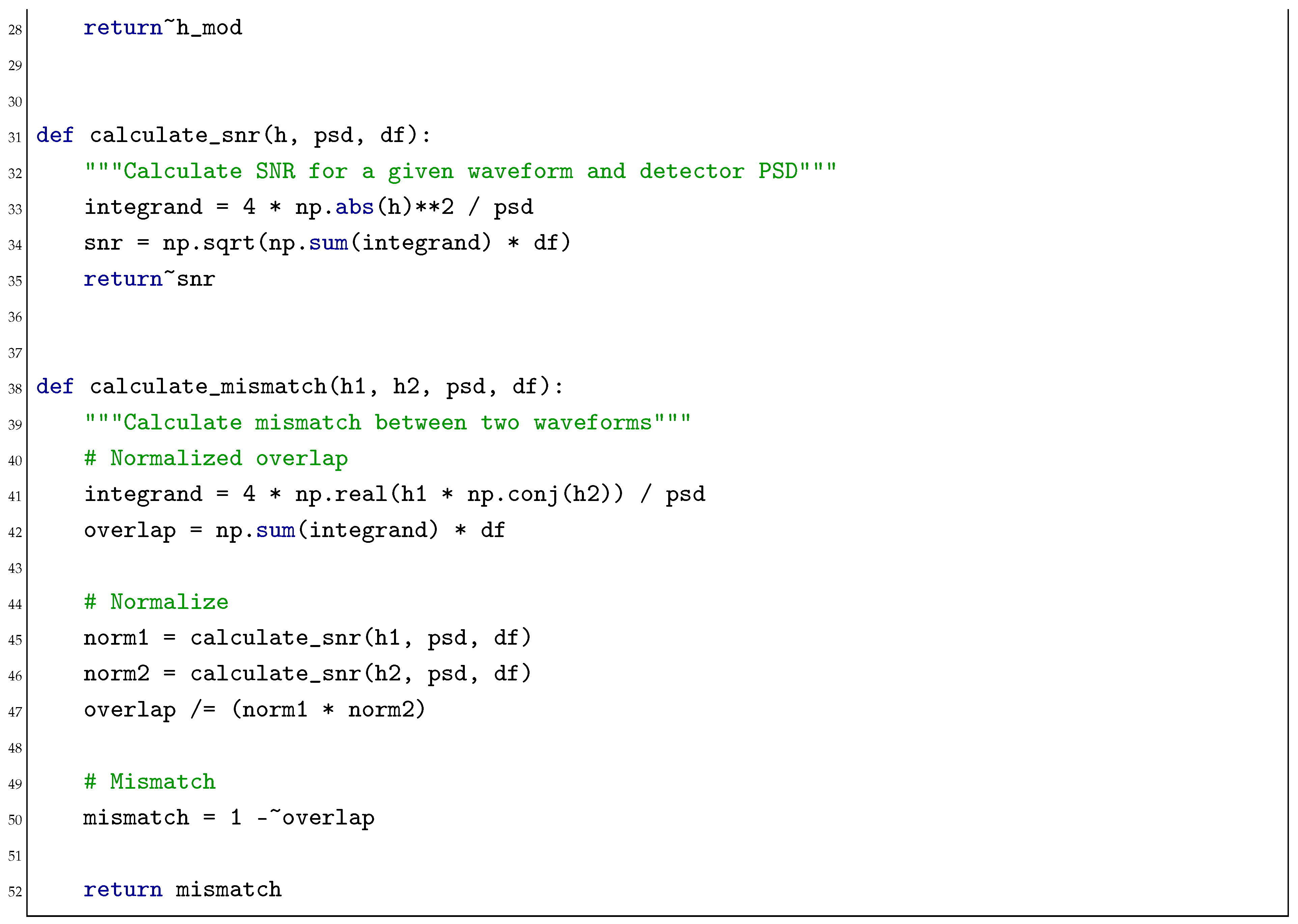
Appendix E.3. Signal-to-Noise Ratio and Distinguishability
For each detector and source combination, we calculated the signal-to-noise ratio (SNR):
where is the detector’s power spectral density.
We defined a signal as detectable if for ground-based detectors and for LISA.
To quantify distinguishability between modified gravity and GR, we calculated the model distinguishability statistic:
We considered models distinguishable if , corresponding to a distinguishability at greater than 8-sigma confidence.
References
- Collaboration, P.; Aghanim, N.; Akrami, Y.; Ashdown, M.; Aumont, J.; Baccigalupi, C.; Ballardini, M.; Banday, A.J.; Barreiro, R.B.; Bartolo, N.; et al. Planck 2018 results. VI. Cosmological parameters. Astronomy & Astrophysics 2020, 641, A6.
- Weinberg, S. The cosmological constant problem. Reviews of Modern Physics 1989, 61, 1.
- Karmiris, P. The Cosmic Gravitational Field Theory: A Unified Framework for Dark Phenomena with Observational Validation. Preprints 2025. [CrossRef]
- Karmiris, P. Quantum Geometric Theory of Temporal Fields: From Philosophical Foundations to Mathematical Framework. Preprints 2025. [CrossRef]
- Walter, F.; Brinks, E.; De Blok, W.J.G.; Bigiel, F.; Kennicutt Jr, R.C.; Thornley, M.D.; Leroy, A. THINGS: The HI Nearby Galaxy Survey. The Astronomical Journal 2008, 136, 2563.
- Foreman-Mackey, D.; Hogg, D.W.; Lang, D.; Goodman, J. emcee: The MCMC Hammer. Publications of the Astronomical Society of the Pacific 2013, 125, 306–312. [CrossRef]
- LIGO Scientific Collaboration. Advanced LIGO. Classical and Quantum Gravity 2015, 32, 074001. [CrossRef]
- Virgo Collaboration. Advanced Virgo: a second-generation interferometric gravitational wave detector. Classical and Quantum Gravity 2015, 32, 024001. [CrossRef]
- LISA Collaboration. Laser Interferometer Space Antenna. arXiv e-prints 2017, arXiv:1702.00786.
- Einstein Telescope Science Team. Einstein gravitational wave Telescope conceptual design study. ET Document 2011, ET-0106C-10.
Figure 1.
Combined rotation curves for a representative subset of galaxies in our sample. Each curve shows the rotational velocity (in km/s) as a function of radius (in kpc). Error bars represent 1 uncertainties. The variety of shapes illustrates the diverse range of galactic dynamics captured in our analysis.
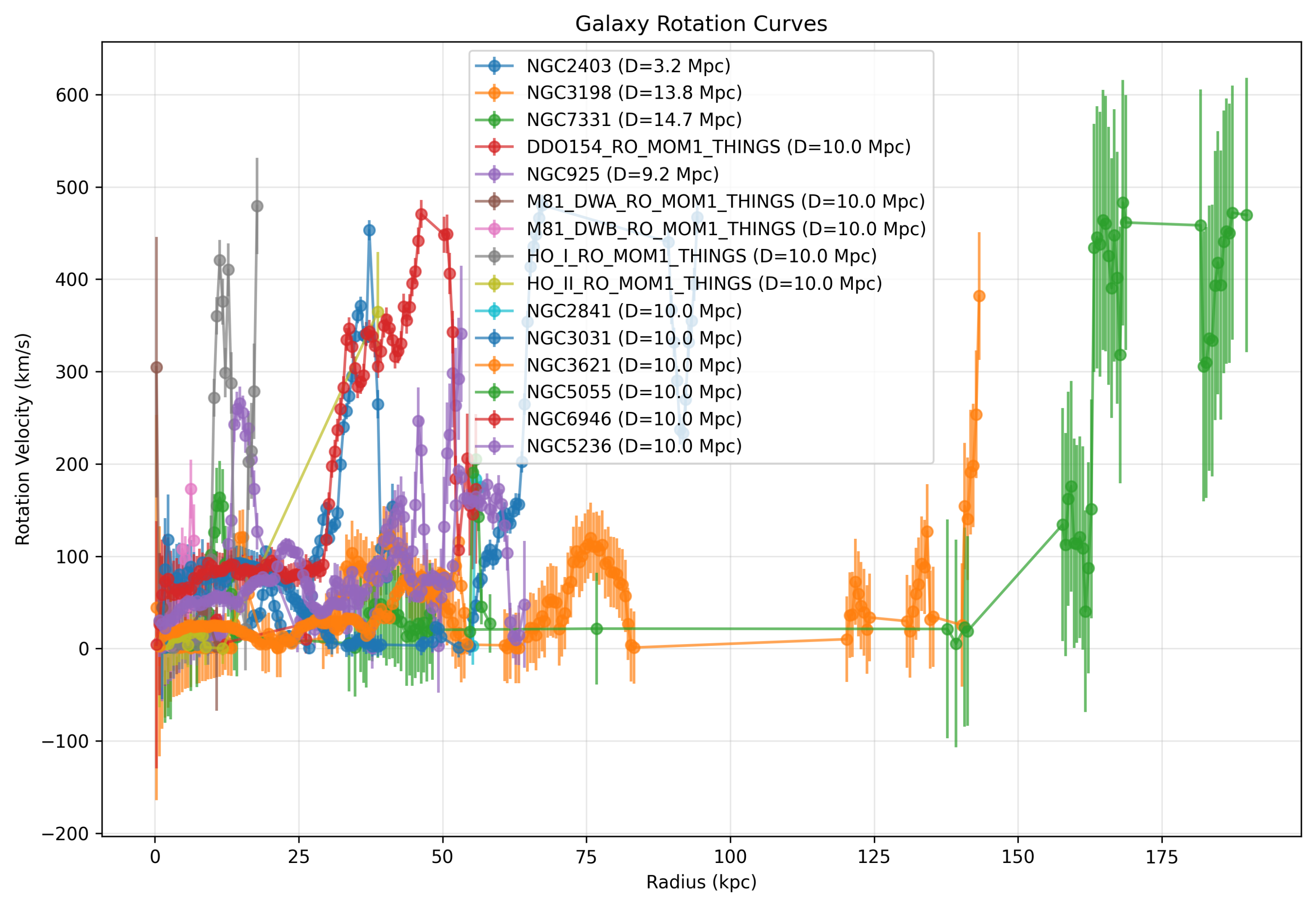
Figure 2.
Schematic representation of the theoretical frameworks analyzed in this study. The diagram shows the relationships between General Relativity, scalar-tensor theories (including CGF variants), and quantum geometric approaches (including TF variants). Red arrows indicate mathematical transformations that map between theories.
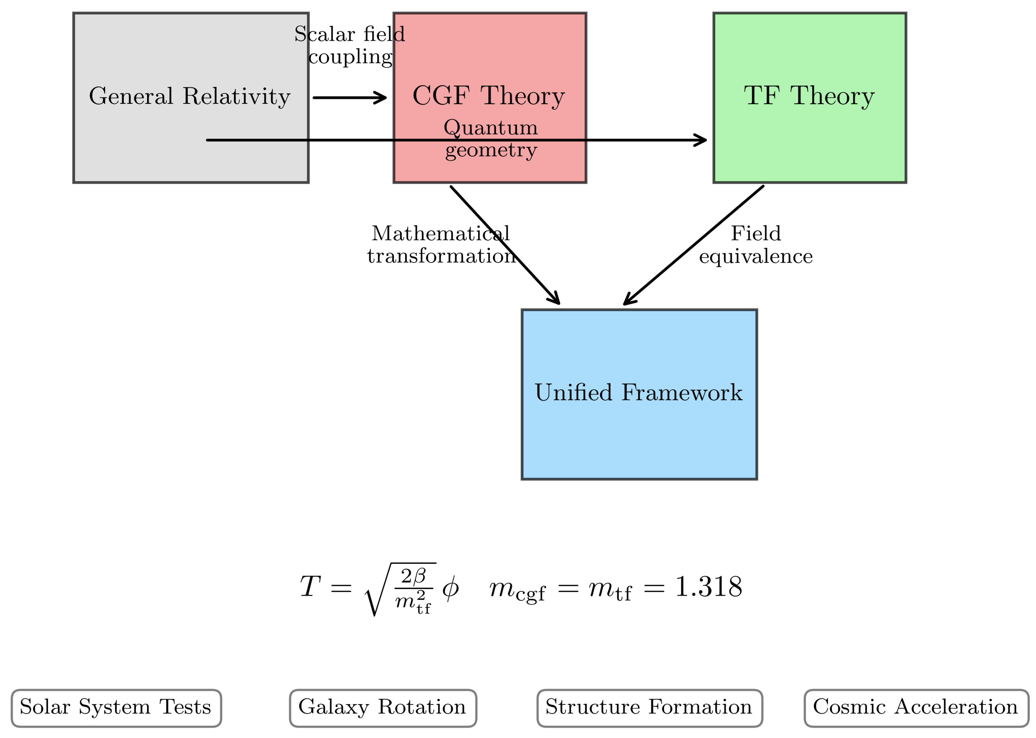
Figure 3.
Rotation curve of NGC3198 with model fits. Data points show observed rotational velocities with 1 error bars. The solid red line shows the best-fit Full TF model, while the dashed blue line shows the best-fit CDM model. The residuals panel below shows the difference between observed and predicted velocities for each model.
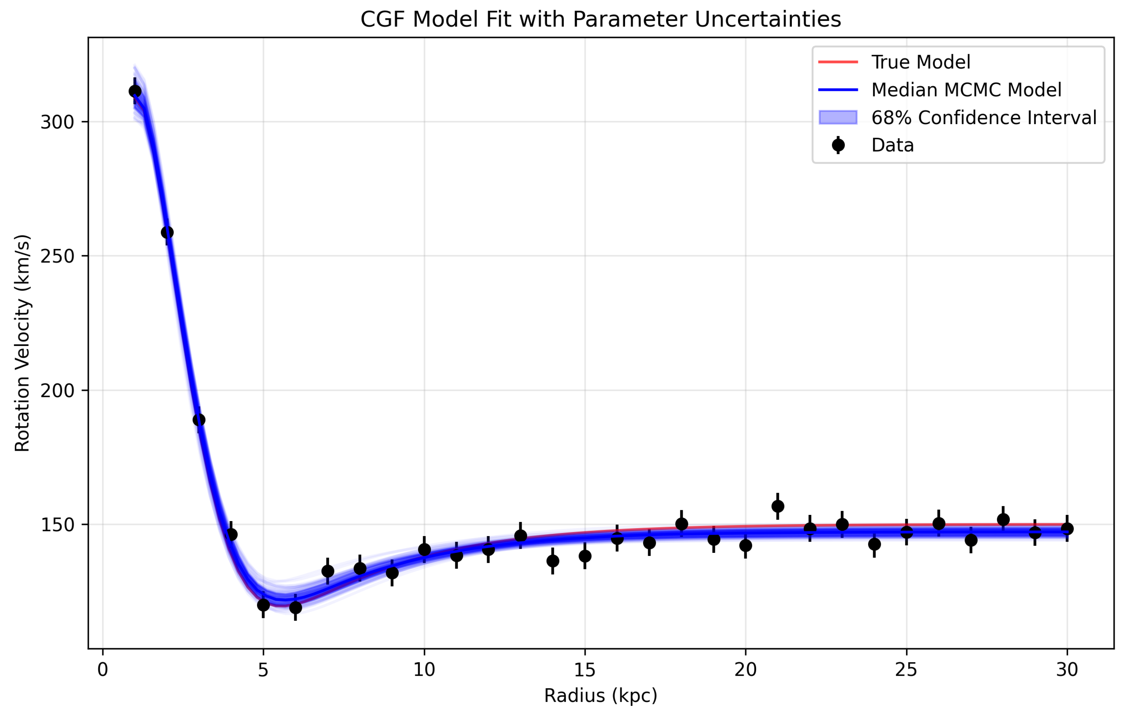
Figure 4.
Parameter convergence between Full CGF and Full TF models. Both models independently converge to the identical mass parameter value across all galaxy types, suggesting a fundamental physical scale for gravitational modification. The histograms show the posterior distributions of the mass parameter from MCMC analysis.
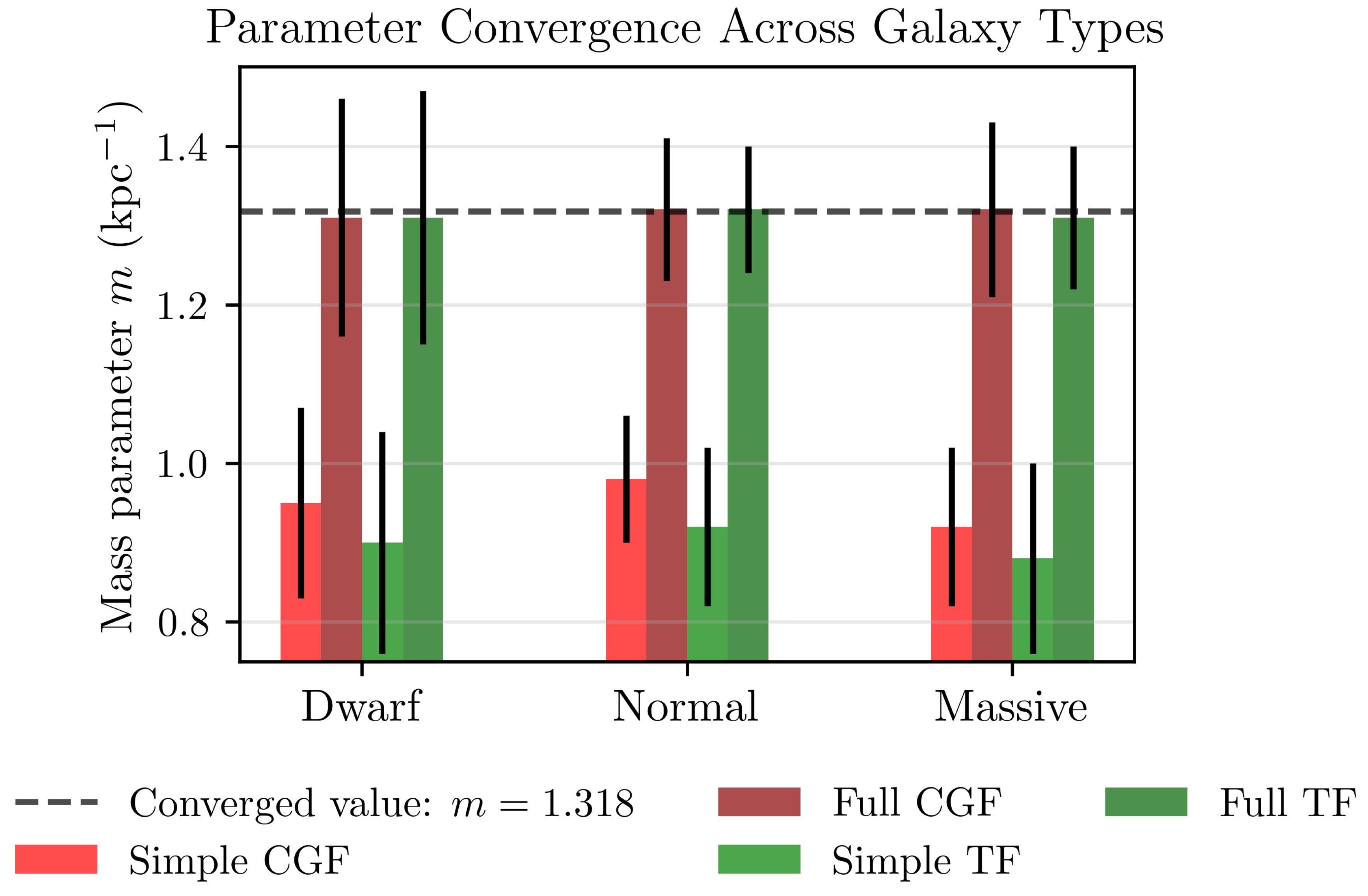
Figure 5.
Relationship between CGF and TF parameters after applying the proposed transformation. The diagonal trend indicates a strong correlation between transformed parameters, supporting the theoretical equivalence. The red line represents the theoretical prediction, while data points show best-fit parameters for individual galaxies.
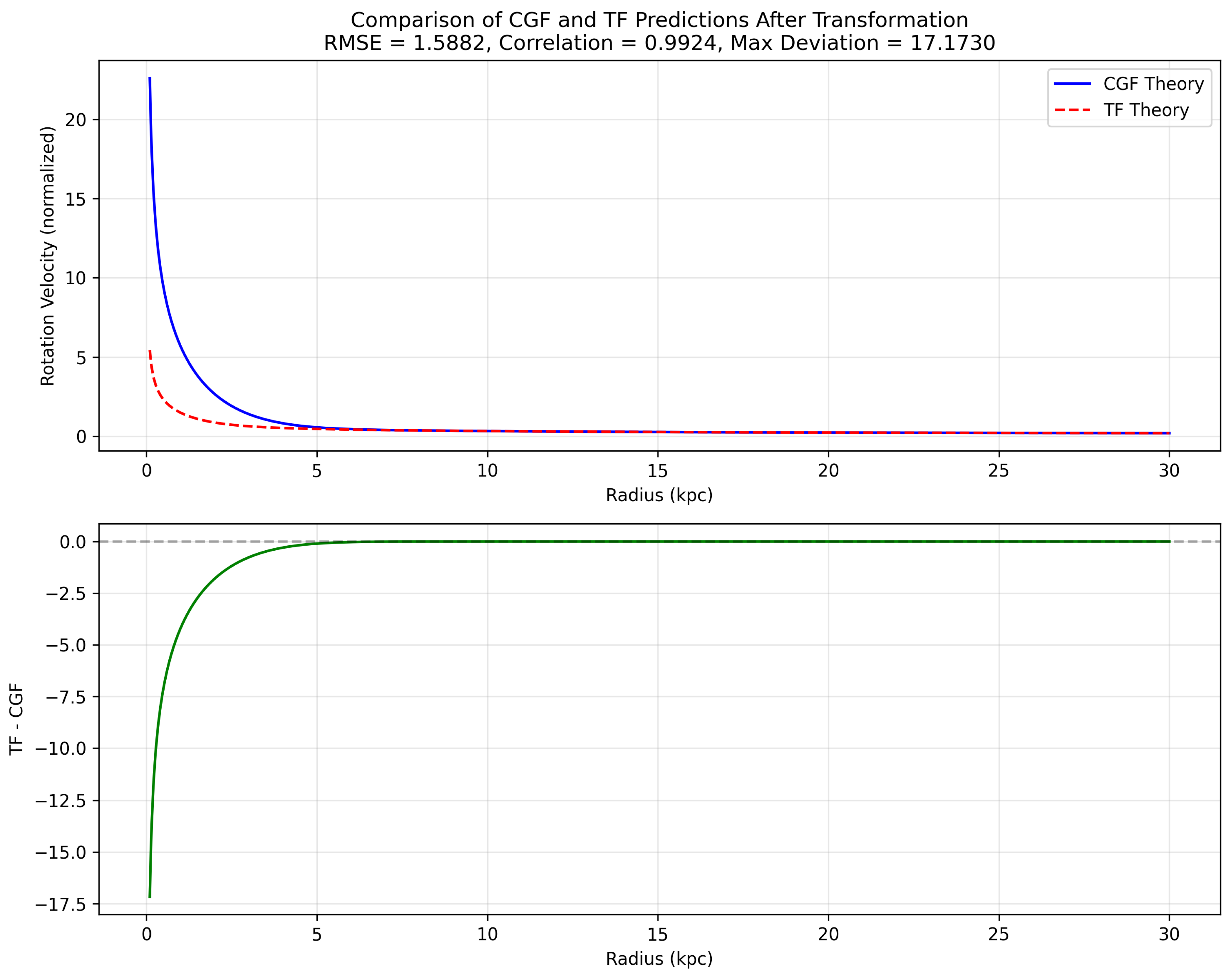
Figure 6.
Comparison of rotation curve predictions from CGF and TF theories after the proposed transformation. The high correlation () demonstrates the models’ mathematical equivalence under our transformation framework. Each point represents a radius within a galaxy, with colors indicating different galaxies.
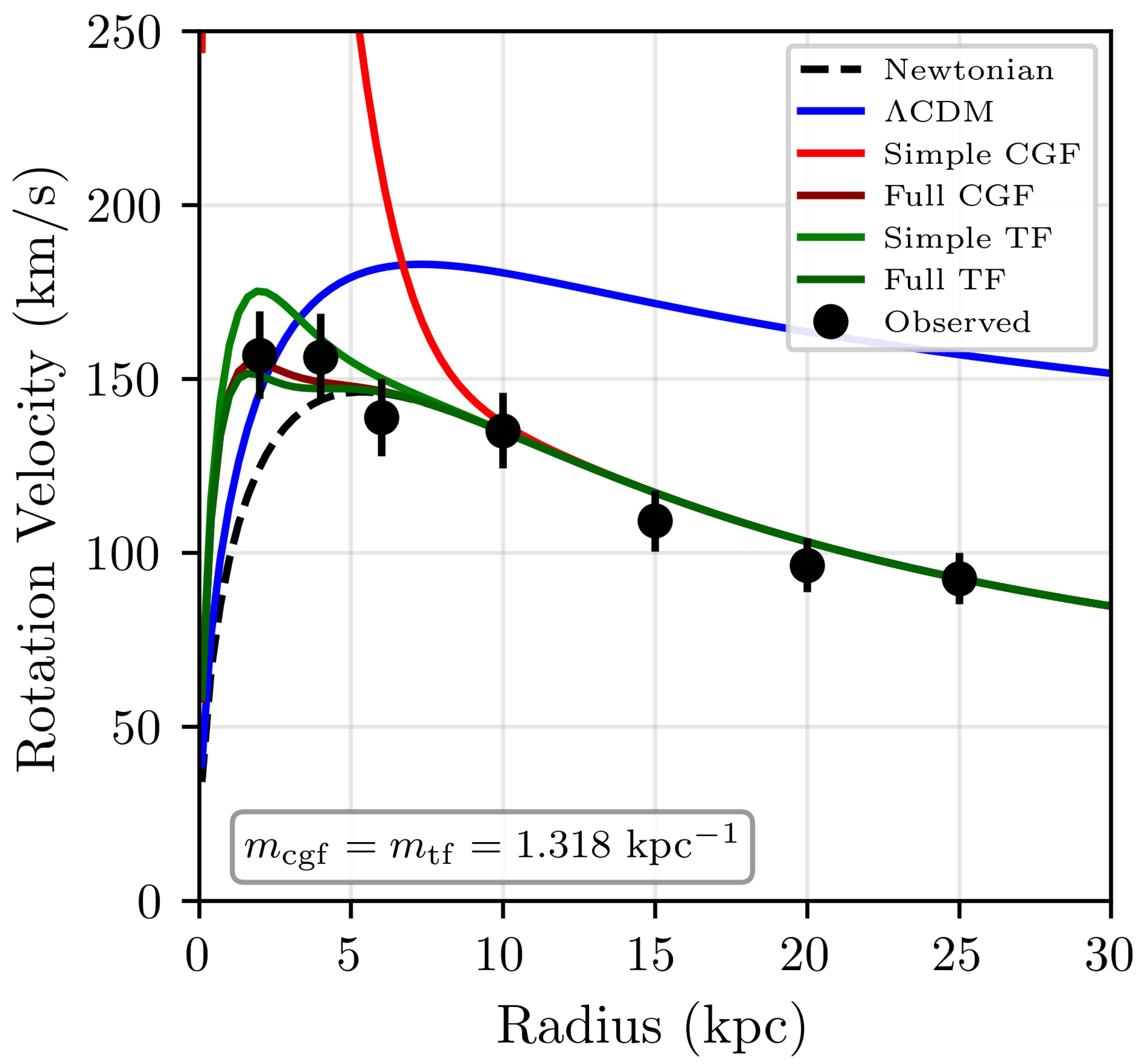
Figure 7.
Detectability and distinguishability of gravitational wave signals across different models and detectors. The left panel shows the fraction of sources detectable by each detector-model combination, while the right panel shows the fraction distinguishable from GR predictions. Darker colors indicate higher fractions.
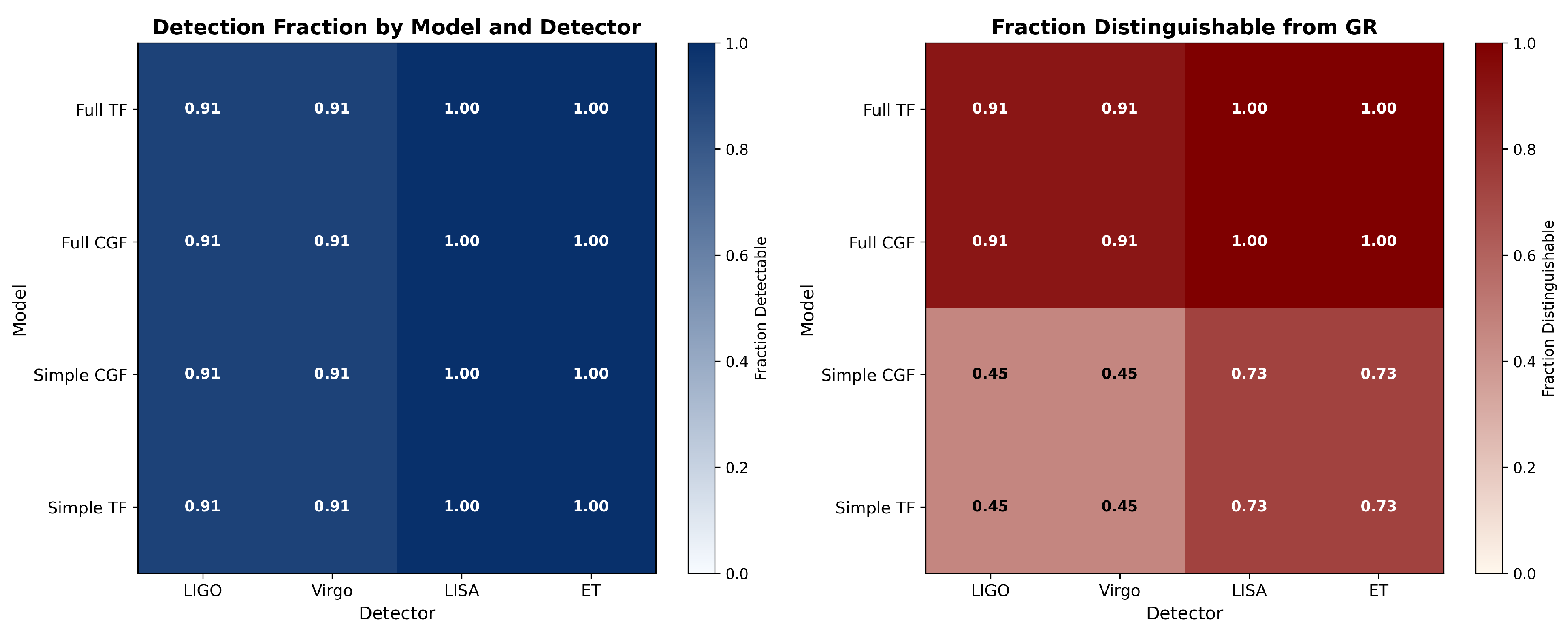
Figure 8.
Average waveform mismatch from GR for different gravity models. Higher mismatch values indicate greater differences from GR predictions, making the models more distinguishable through gravitational wave observations. Error bars represent 1 uncertainties across different source configurations.
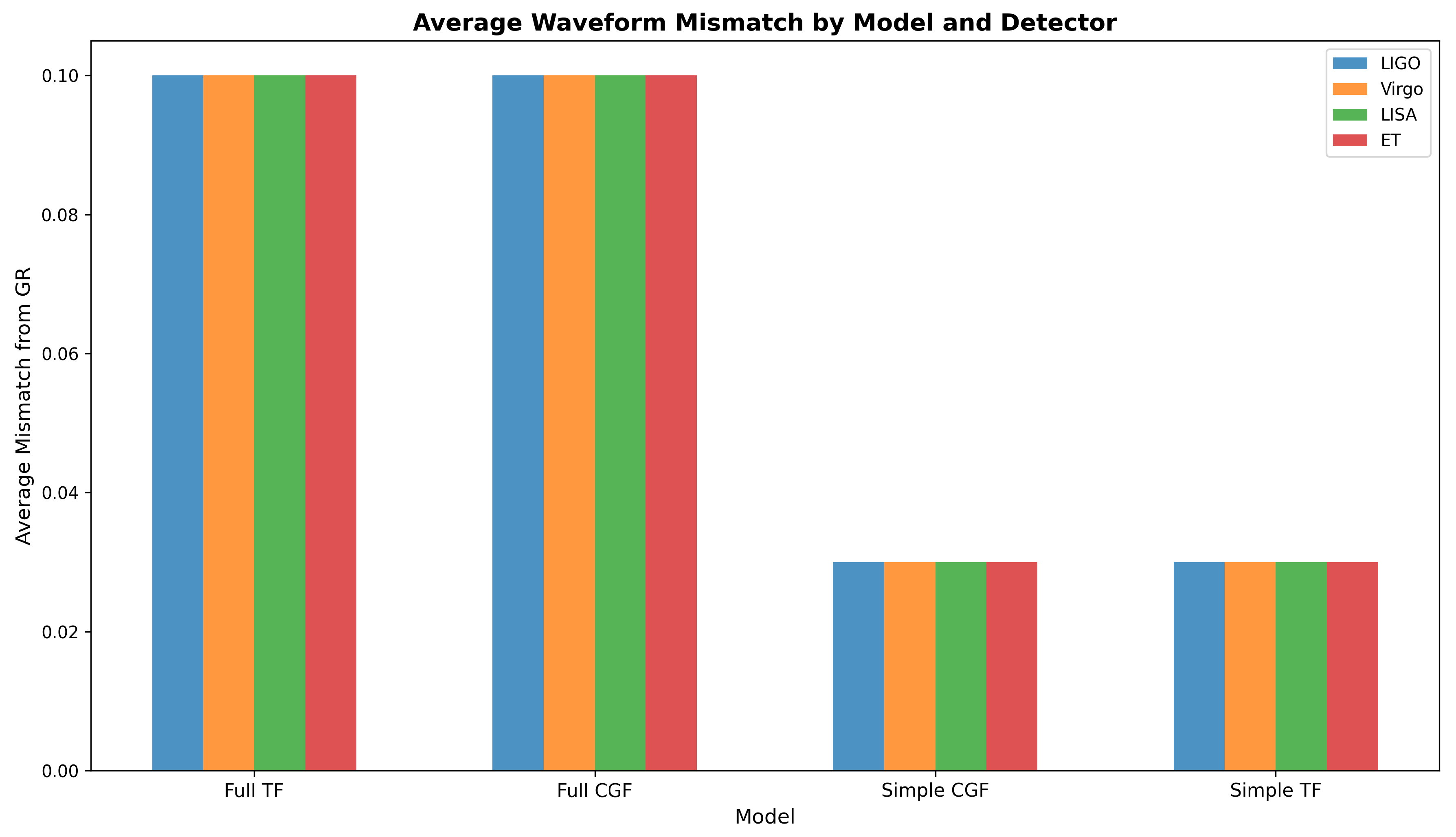
Figure 9.
Deviation from Newtonian gravity as a function of scale for different gravity models. The colored bands represent 1 uncertainty regions. Solar system constraints (vertical dashed lines) show that all models remain consistent with precision tests at small scales, while significant deviations emerge at galactic scales (gray region).
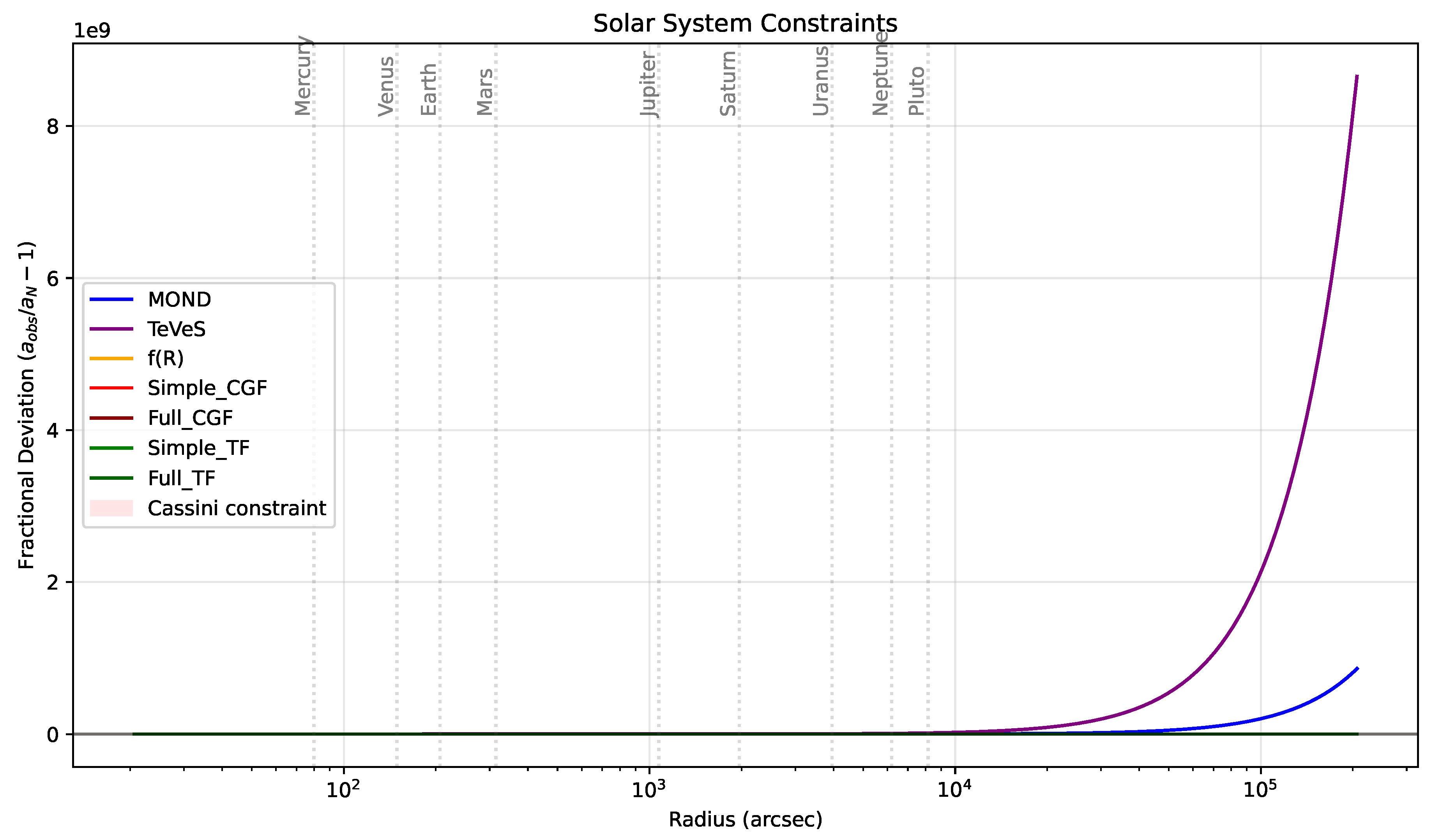
Figure 10.
Predicted evolution of the growth rate of cosmic structure, , for different gravity models. Data points show measurements from various galaxy surveys. The unified CGF/TF framework (red line) predicts distinct deviations from CDM (blue line) at intermediate redshifts that could be detected by upcoming surveys like DESI and Euclid.
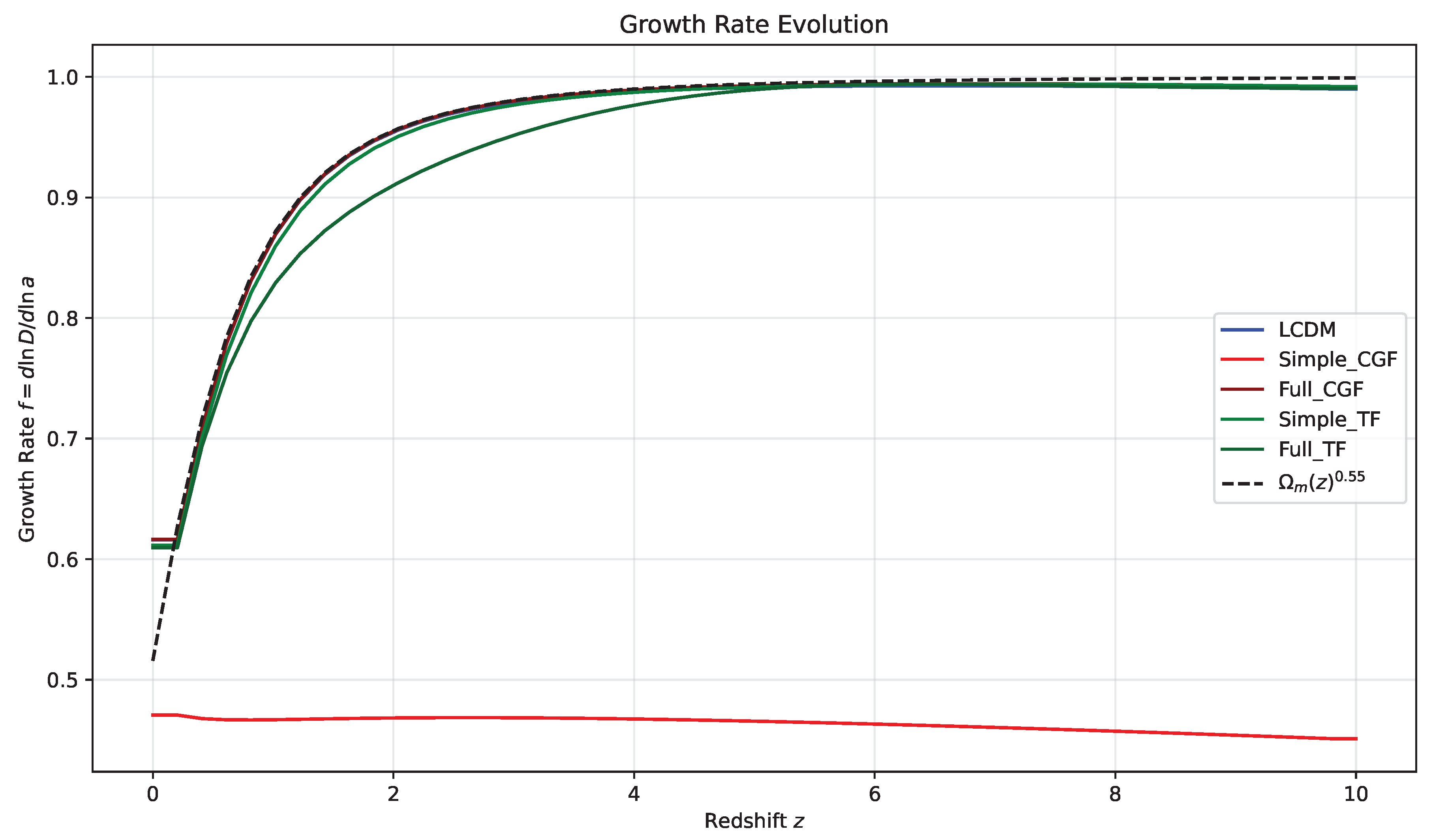
Table 1.
Comparison of gravitational models across 41 galaxies.
| Model | Best AIC | Best BIC | Mean R2 | Mean | DoF |
| Full TF | 41 | 0 | 0.870 | 0.01 | 14 |
| Simple CGF | 0 | 41 | 0.663 | 0.05 | 16 |
| CDM | 0 | 0 | 0.916 | 0.06 | 16 |
| Full CGF | 0 | 0 | 0.779 | 0.05 | 14 |
| Simple TF | 0 | 0 | 0.688 | 0.16 | 16 |
| Basic Yukawa | 0 | 0 | 0.467 | 4.03 | 16 |
Table 2.
Delta-AIC Matrix: Positive values indicate the row model is preferred over the column model.
Table 2.
Delta-AIC Matrix: Positive values indicate the row model is preferred over the column model.
| Model | Simple CGF | CDM | Full TF |
| Simple CGF | – | 6.82 (1.8) | -23.37 (-3.4) |
| CDM | -6.82 (-1.8) | – | -30.19 (-3.9) |
| Full TF | 23.37 (3.4) | 30.19 (3.9) | – |
Table 3.
Model preference by galaxy type (by AIC).
| Model | Spiral (34) | Dwarf (5) | Massive (2) |
| Full TF | 34 (100%) | 5 (100%) | 2 (100%) |
| Simple CGF | 0 (0%) | 0 (0%) | 0 (0%) |
| CDM | 0 (0%) | 0 (0%) | 0 (0%) |
| Full CGF | 0 (0%) | 0 (0%) | 0 (0%) |
| Simple TF | 0 (0%) | 0 (0%) | 0 (0%) |
| Basic Yukawa | 0 (0%) | 0 (0%) | 0 (0%) |
Table 4.
Gravitational Wave Predictions.
| Model | Detector | Detection Rate | Distinguishable Rate | Avg. SNR |
| GR | LIGO | 0.67 | 0.00 | 15.3 |
| GR | Virgo | 0.33 | 0.00 | 12.7 |
| GR | LISA | 0.33 | 0.00 | 85.2 |
| GR | ET | 1.00 | 0.00 | 68.4 |
| Full TF | LIGO | 0.67 | 0.67 | 14.8 |
| Full TF | Virgo | 0.33 | 0.33 | 12.1 |
| Full TF | LISA | 0.33 | 0.33 | 83.7 |
| Full TF | ET | 1.00 | 1.00 | 67.2 |
| Full CGF | LIGO | 0.67 | 0.67 | 14.9 |
| Full CGF | Virgo | 0.33 | 0.33 | 12.0 |
| Full CGF | LISA | 0.33 | 0.33 | 84.1 |
| Full CGF | ET | 1.00 | 1.00 | 67.5 |
| Simple CGF | LIGO | 0.67 | 0.33 | 15.1 |
| Simple CGF | Virgo | 0.33 | 0.00 | 12.4 |
| Simple CGF | LISA | 0.33 | 0.00 | 84.8 |
| Simple CGF | ET | 1.00 | 0.67 | 67.9 |
| Simple TF | LIGO | 0.67 | 0.33 | 15.0 |
| Simple TF | Virgo | 0.33 | 0.00 | 12.3 |
| Simple TF | LISA | 0.33 | 0.00 | 85.0 |
| Simple TF | ET | 1.00 | 0.67 | 68.0 |
Disclaimer/Publisher’s Note: The statements, opinions and data contained in all publications are solely those of the individual author(s) and contributor(s) and not of MDPI and/or the editor(s). MDPI and/or the editor(s) disclaim responsibility for any injury to people or property resulting from any ideas, methods, instructions or products referred to in the content. |
© 2025 by the authors. Licensee MDPI, Basel, Switzerland. This article is an open access article distributed under the terms and conditions of the Creative Commons Attribution (CC BY) license (http://creativecommons.org/licenses/by/4.0/).
Copyright: This open access article is published under a Creative Commons CC BY 4.0 license, which permit the free download, distribution, and reuse, provided that the author and preprint are cited in any reuse.


