The Cosmic Gravitational Field Theory: A Unified Framework for Dark Phenomena with Observational Validation

1. Introduction

Contemporary cosmology faces several fundamental challenges that suggest our understanding of gravity at various scales may be incomplete. The standard cosmological model, $\mathrm{\Lambda }$CDM, has been remarkably successful in explaining a wide range of observations, from the cosmic microwave background to large-scale structure formation [1]. However, this success comes at the cost of introducing two mysterious components: dark matter and dark energy, which together constitute approximately 95% of the energy content of the Universe [2,3].

Despite decades of experimental searches, dark matter particles have eluded direct detection [2], while the cosmological constant, representing dark energy, suffers from theoretical inconsistencies that have not been resolved satisfactorily [4,5]. These persistent difficulties motivate the exploration of alternative theoretical frameworks that might explain observational data without requiring these enigmatic components.

Several approaches to modified gravity have emerged as potential alternatives to $\mathrm{\Lambda }$CDM, including Modified Newtonian Dynamics (MOND) [6], Tensor-Vector-Scalar (TeVeS) theory [7], $f\left(R\right)$ gravity [8], and various scalar-tensor theories [9]. While each of these frameworks has shown success in addressing specific phenomena, they often struggle to provide a comprehensive explanation across all observational scales.

In this paper, we introduce the Cosmic Gravitational Field (CGF) theory—a novel approach that introduces a gravity amplification field which enhances the standard gravitational interaction. Unlike conventional modified gravity theories, the CGF framework is built on the principle that gravity’s strength can be modulated by a dynamical field that couples to the standard gravitational sector.

The structure of this paper is as follows: Section 2 outlines the philosophical foundations of CGF theory. Section 3 presents the theoretical framework, including the action principle, field equations, and physical interpretation. Section 4 compares CGF with other cosmological theories. Section 5 details our approach to testing CGF against observational data. Section 6 presents the results of our analysis of galaxy rotation curves. Section 7 discusses the strengths and limitations of the theory, including falsifiability criteria. Finally, Section 8 explores the implications of our findings and potential future directions.

2. Philosophical Foundations

2.1. From Spacetime to Fields: A Paradigm Shift

The CGF theory represents a significant paradigm shift in our conceptualization of gravity. While General Relativity (GR) describes gravity as the curvature of spacetime, CGF introduces an additional layer—a field that amplifies the gravitational interaction. This approach echoes historical transitions in physics, such as the shift from action-at-a-distance to field theories in electromagnetism [10].

This paradigm shift allows us to reconsider the nature of the "dark" phenomena in cosmology. Rather than invoking new forms of matter or energy, CGF suggests that what appears as dark matter and dark energy might be manifestations of the same underlying field that modulates the strength of gravity across different scales.

2.2. The Active Nature of Gravity

The CGF framework advances a view of gravity as fundamentally active rather than passive. Instead of treating spacetime as a fixed arena that merely responds to matter and energy, CGF posits that the gravitational interaction itself possesses dynamic properties that can vary across different environments.

This perspective aligns with Wheeler’s vision of "spacetime telling matter how to move, and matter telling spacetime how to curve" [11], but extends it to include a feedback mechanism where the strength of this communication can itself vary based on physical conditions.

2.3. Unification of Scales: Bridging Quantum and Cosmic Realms

A persistent challenge in theoretical physics is the reconciliation of quantum mechanics with gravity. The CGF approach offers a potential bridge between these scales by introducing a field that operates at galactic and cosmological scales but whose origins might be traced to quantum gravitational effects.

The gravity amplification field could emerge from quantum fluctuations of spacetime, providing a phenomenological connection between quantum gravity and large-scale cosmological phenomena without requiring a complete theory of quantum gravity. This resonates with holographic principles that suggest connections between different scales of physical reality [12,13].

2.4. Relational vs. Absolute Views of Spacetime

CGF theory embraces a relational view of spacetime, where gravitational effects cannot be separated from the physical context in which they occur. The strength of gravity is not an absolute quantity but depends on the distribution of matter and energy, as well as the state of the gravity amplification field.

This perspective draws inspiration from Leibniz and Mach, who emphasized that physical properties should be understood in terms of relationships rather than absolute quantities [14]. In CGF, the effective gravitational interaction emerges from the relationship between ordinary matter, spacetime curvature, and the amplification field.

3. Theoretical Framework

3.1. Action Principle and Field Equations

The CGF theory is formulated based on a modification of the Einstein-Hilbert action, incorporating a scalar field $\varphi$ that modulates the strength of the gravitational interaction. The complete action for the CGF theory can be expressed as:

$$\begin{array}{cc}\hfill S& =\int d^{4}x\sqrt{-g}\left[{\displaystyle \frac{1}{16\pi G}}R+{\mathcal{L}}_{\varphi }+{\mathcal{L}}_m\right]\hfill \end{array}$$

(1)

$$\begin{array}{cc}\hfill {\mathcal{L}}_{\varphi }& =-{\displaystyle \frac{1}{2}}{g}^{\mu \nu }{\partial }_{\mu }\varphi {\partial }_{\nu }\varphi -V\left(\varphi \right)+f\left(\varphi \right)R\hfill \end{array}$$

(2)

$$\begin{array}{cc}\hfill G_{\mu \nu }+H_{\mu \nu }& =8\pi G{T}_{\mu \nu }\hfill \end{array}$$

(3)

$$\begin{array}{cc}\hfill \square \varphi -V^{\prime }\left(\varphi \right)+f^{\prime }\left(\varphi \right)R& =0\hfill \end{array}$$

(4)

where R is the Ricci scalar, G is Newton’s gravitational constant, g is the determinant of the metric tensor, ${\mathcal{L}}_{\varphi }$ is the Lagrangian density of the scalar field, and ${\mathcal{L}}_m$ is the Lagrangian density of ordinary matter.

The scalar field Lagrangian takes the form shown in the second equation above, where $V\left(\varphi \right)$ is the potential of the scalar field, and $f\left(\varphi \right)$ represents the coupling between the scalar field and the Ricci scalar, which modulates the strength of gravity.

Derivation of Field Equations

Starting with the complete action, we perform a variation with respect to the metric $g_{\mu \nu }$ to derive the field equations. The variation of the action yields:

$\delta S=\int d^{4}x\left[{\displaystyle \frac{\delta \left(\sqrt{-g}\right)}{16\pi G}}R+{\displaystyle \frac{\sqrt{-g}}{16\pi G}}\delta R+\delta \left(\sqrt{-g}{\mathcal{L}}_{\varphi }\right)+\delta \left(\sqrt{-g}{\mathcal{L}}_m\right)\right]$

For the variation of the metric determinant, we use the identity $\delta \left(\sqrt{-g}\right)=-{\displaystyle \frac{1}{2}}\sqrt{-g}{g}_{\mu \nu }\delta g^{\mu \nu }$. The variation of the Ricci scalar can be expanded as:

$\delta R=\delta \left(g^{\mu \nu }{R}_{\mu \nu }\right)=\delta g^{\mu \nu }{R}_{\mu \nu }+g^{\mu \nu }\delta R_{\mu \nu }$

The variation of the Ricci tensor involves derivatives of the connection coefficients:

$\delta R_{\mu \nu }={\nabla }_{\alpha }\delta {\Gamma }_{\mu \nu }^{\alpha }-{\nabla }_{\nu }\delta {\Gamma }_{\mu \alpha }^{\alpha }$

After integration by parts and applying the divergence theorem, the second term in the Ricci scalar variation yields:

$\int d^{4}x\sqrt{-g}{g}^{\mu \nu }\delta R_{\mu \nu }=\int d^{4}x\sqrt{-g}(g^{\mu \nu }\square \delta g_{\mu \nu }-{\nabla }_{\mu }{\nabla }_{\nu }\delta g^{\mu \nu })$

The scalar field contribution to the variation comes from both the direct kinetic and potential terms as well as the non-minimal coupling term $f\left(\varphi \right)R$. Explicitly:

$\delta \left(\sqrt{-g}{\mathcal{L}}_{\varphi }\right)=\delta \left[\sqrt{-g}\left(-{\displaystyle \frac{1}{2}}{g}^{\mu \nu }{\partial }_{\mu }\varphi {\partial }_{\nu }\varphi -V\left(\varphi \right)+f\left(\varphi \right)R\right)\right]$

Expanding this yields terms involving $\delta g^{\mu \nu }$ and terms involving $f\left(\varphi \right)\delta R$ which must be handled similarly to the first term in the action.

Collecting all terms with $\delta g^{\mu \nu }$ gives us:

$$\begin{array}{c}\hfill \int d^{4}x\sqrt{-g}\left[{\displaystyle \frac{1}{16\pi G}}\left(R_{\mu \nu }-{\displaystyle \frac{1}{2}}{g}_{\mu \nu }R\right)+{\nabla }_{\mu }{\nabla }_{\nu }f\left(\varphi \right)-g_{\mu \nu }\square f\left(\varphi \right)\right.\\ \hfill \left.-{\displaystyle \frac{1}{2}}{g}_{\mu \nu }{g}^{\alpha \beta }{\partial }_{\alpha }\varphi {\partial }_{\beta }\varphi +{\partial }_{\mu }\varphi {\partial }_{\nu }\varphi +g_{\mu \nu }V\left(\varphi \right)\right]\delta g^{\mu \nu }.\end{array}$$

Using the definition of the energy-momentum tensor $T_{\mu \nu }$ from the matter Lagrangian:

$T_{\mu \nu }=-{\displaystyle \frac{2}{\sqrt{-g}}}{\displaystyle \frac{\delta \left(\sqrt{-g}{\mathcal{L}}_m\right)}{\delta g^{\mu \nu }}}$

We obtain the field equations in their final form:

$G_{\mu \nu }+H_{\mu \nu }=8\pi G{T}_{\mu \nu }$

where $H_{\mu \nu }$ explicitly contains all terms related to the scalar field:

$H_{\mu \nu }={\nabla }_{\mu }{\nabla }_{\nu }f\left(\varphi \right)-g_{\mu \nu }\square f\left(\varphi \right)-{\displaystyle \frac{1}{2}}{g}_{\mu \nu }{g}^{\alpha \beta }{\partial }_{\alpha }\varphi {\partial }_{\beta }\varphi +{\partial }_{\mu }\varphi {\partial }_{\nu }\varphi +g_{\mu \nu }V\left(\varphi \right)$

Similarly, by varying the action with respect to the scalar field $\varphi$, we obtain the equation of motion for the scalar field:

$\square \varphi -V^{\prime }\left(\varphi \right)+f^{\prime }\left(\varphi \right)R=0$

where primes denote derivatives with respect to $\varphi$.

By varying the action with respect to the metric $g_{\mu \nu }$ and the scalar field $\varphi$, we obtain the field equations shown in the third and fourth equations, where $G_{\mu \nu }$ is the Einstein tensor, $H_{\mu \nu }$ contains the modifications due to the scalar field, $T_{\mu \nu }$ is the energy-momentum tensor of ordinary matter, □ is the d’Alembertian operator, and primes denote derivatives with respect to $\varphi$.

3.2. The Simple CGF Model Derivation

The Simple CGF model, which we focus on in this paper, employs a specific form for the coupling function $f\left(\varphi \right)$ and potential $V\left(\varphi \right)$ that leads to a Yukawa-like modification of the gravitational potential at galactic scales while allowing for cosmological acceleration.

For the Simple CGF model, we choose the following functional forms:

$f\left(\varphi \right)={\displaystyle \frac{1}{16\pi G}}+{\displaystyle \frac{\beta {\varphi }^2}{2}}$$V\left(\varphi \right)={\displaystyle \frac{m_{\mathrm{cgf}}^2{\varphi }^2}{2}}$

where $\beta$ is a coupling constant related to $\alpha$ in our final equations, and $m_{\mathrm{cgf}}$ is the effective mass of the scalar field. These specific forms are chosen based on their simplicity and their capacity to generate the required modification to gravity at galactic scales. The quadratic coupling ensures that the modification grows with the scalar field strength, while the mass term in the potential provides a characteristic scale to the modification.

In the weak-field, non-relativistic limit relevant for galaxy dynamics, we can approximate the metric as a small perturbation around Minkowski space: $g_{\mu \nu }={\eta }_{\mu \nu }+h_{\mu \nu }$ with $|h_{\mu \nu }|\ll 1$. Under these assumptions, the field equations can be linearized.

Starting with the field equations derived in Section 3.1, and considering the static case where time derivatives vanish, the scalar field equation becomes:

${\nabla }^2\varphi -m_{\mathrm{cgf}}^2\varphi +\beta \varphi R=0$

For a spherically symmetric mass distribution in the weak field limit, the Ricci scalar is proportional to the trace of the energy-momentum tensor: $R\approx -8\pi G\rho$, where $\rho$ is the mass density. Substituting this into the scalar field equation:

${\nabla }^2\varphi -m_{\mathrm{cgf}}^2\varphi -8\pi G\beta \varphi \rho =0$

For a point mass M at the origin, $\rho =M{\delta }^3\left(\mathbf{r}\right)$, the solution to this equation takes the form:

$\varphi \left(r\right)={\varphi }_0{\displaystyle \frac{e^{-m_{\mathrm{cgf}}r}}{r}}$

where ${\varphi }_0$ is determined by the source term. This solution shows that the scalar field has a Yukawa-like profile around a massive body.

The modified gravitational potential can be derived from the $\left(00\right)$ component of the field equations, which in the weak field limit gives:

${\nabla }^2\mathrm{\Phi }=4\pi G\rho -{\nabla }^2\left(f\left(\varphi \right)\right)$

For our choice of $f\left(\varphi \right)$ and the solution for $\varphi \left(r\right)$, this results in a modified potential:

$\mathrm{\Phi }\left(r\right)=-{\displaystyle \frac{GM}{r}}(1+\alpha e^{-m_{\mathrm{cgf}}r})$

where $\alpha =2\beta /\left(16\pi G{m}_{\mathrm{cgf}}^2\right)$ is the coupling strength parameter that determines the magnitude of the modification.

Taking the gradient of this potential gives the modified gravitational force:

$F\left(r\right)=-{\displaystyle \frac{d\mathrm{\Phi }}{dr}}=-{\displaystyle \frac{GM}{r^2}}(1+\alpha e^{-m_{\mathrm{cgf}}r}(1+m_{\mathrm{cgf}}r))$

For a test particle in a circular orbit, the centripetal acceleration equals the gravitational force, giving:

${\displaystyle \frac{v^2}{r}}={\displaystyle \frac{GM}{r^2}}(1+\alpha e^{-m_{\mathrm{cgf}}r}(1+m_{\mathrm{cgf}}r))$

Solving for $v^2\left(r\right)$ yields the rotation curve formula:

$$\begin{array}{cc}\hfill \mathrm{\Phi }\left(r\right)& =-{\displaystyle \frac{GM}{r}}(1+\alpha e^{-m_{\mathrm{cgf}}r})\hfill \end{array}$$

(5)

$$\begin{array}{cc}\hfill F\left(r\right)& =-{\displaystyle \frac{d\mathrm{\Phi }}{dr}}=-{\displaystyle \frac{GM}{r^2}}(1+\alpha e^{-m_{\mathrm{cgf}}r}(1+m_{\mathrm{cgf}}r))\hfill \end{array}$$

(6)

3.3. The Gravity Amplification Mechanism

The central concept of CGF theory is the gravity amplification mechanism, whereby the scalar field $\varphi$ enhances the gravitational interaction in specific regimes without requiring dark matter. This amplification arises from the non-minimal coupling between the scalar field and the Ricci scalar, represented by the term $f\left(\varphi \right)R$ in the action.

In regions with significant matter density, such as galaxies, the scalar field configuration adjusts to enhance gravity, effectively mimicking the presence of dark matter. The strength of this enhancement depends on both the local matter distribution and the global properties of the field.

The amplification mechanism operates on galactic scales where the modified gravitational potential produces rotation curves that match observations without requiring dark matter. The parameter $m_{\mathrm{cgf}}$ controls the characteristic scale of this modification, while the coupling strength $\alpha$ determines its magnitude.

3.4. Temporal Field Dynamics

A distinctive feature of the CGF theory is its incorporation of temporal dynamics in the scalar field. The evolution of $\varphi$ over cosmic time provides a natural connection to dark energy phenomena and cosmic acceleration.

In the cosmological context with the Friedmann-Lemaître-Robertson-Walker (FLRW) metric, the scalar field equation of motion takes the form:

$$\ddot{\varphi }+3H\dot{\varphi }+V^{\prime }\left(\varphi \right)-f^{\prime }\left(\varphi \right)R=0$$

(7)

where H is the Hubble parameter, dots represent derivatives with respect to cosmic time, and R is now the cosmological Ricci scalar, which in FLRW spacetime is:

$$R=6\left(\dot{H}+2H^2+{\displaystyle \frac{k}{a^2}}\right)$$

(8)

For a spatially flat universe ($k=0$), this simplifies to $R=6(\dot{H}+2H^2)$.

The form of the coupling function $f\left(\varphi \right)$ and potential $V\left(\varphi \right)$ for cosmological evolution is the same as that used at galactic scales:

$$f\left(\varphi \right)={\displaystyle \frac{1}{16\pi G}}+{\displaystyle \frac{\beta {\varphi }^2}{2}}$$

(9)

$$V\left(\varphi \right)={\displaystyle \frac{m_{\mathrm{cgf}}^2{\varphi }^2}{2}}$$

(10)

where $\beta$ is directly related to the coupling strength $\alpha$ in the rotation curve formalism by $\alpha =2\beta /\left(16\pi G{m}_{\mathrm{cgf}}^2\right)$. This ensures consistency between galactic and cosmological scales.

The dynamics of this system can be numerically integrated using the modified Friedmann equations:

$$H^2={\displaystyle \frac{8\pi G}{3}}{\rho }_m+{\displaystyle \frac{1}{3}}\left({\displaystyle \frac{1}{2}}{\dot{\varphi }}^2+V\left(\varphi \right)-6H\dot{f}\left(\varphi \right)+6H^{2}f\left(\varphi \right)\right)$$

(11)

$$\dot{H}=-4\pi G{\rho }_m-{\displaystyle \frac{1}{2}}{\dot{\varphi }}^2+H\dot{f}\left(\varphi \right)-\ddot{f}\left(\varphi \right)$$

(12)

We employ a fourth-order Runge-Kutta integration scheme to solve this coupled system of non-linear differential equations with appropriate initial conditions.

In the early universe ($z\gtrsim 100$), the high curvature ($R\gg 0$) dominates the scalar field equation through the $f^{\prime }\left(\varphi \right)R$ term, keeping the field near its minimum potential value. This makes the field’s contribution to cosmic dynamics negligible, and the universe expands like standard matter-dominated $\mathrm{\Lambda }$CDM. As the universe expands and R decreases during the matter-dominated era, the scalar field’s evolution becomes more pronounced.

The key transition occurs as R approaches the value $\sim m_{\mathrm{cgf}}^2/\beta$. Around redshift $z\approx 0.7$, the potential term $V^{\prime }\left(\varphi \right)$ in the scalar field equation becomes comparable in magnitude to the coupling term $f^{\prime }\left(\varphi \right)R$, enabling the scalar field to significantly deviate from its potential minimum. Concurrently, in the Friedmann equations, the modified gravity term $6H^{2}f\left(\varphi \right)$, which is initially subdominant, begins to overtake the matter density term ${\displaystyle \frac{8\pi G}{3}}{\rho }_m$, causing the universe to transition from decelerated to accelerated expansion. This transition corresponds to a change from matter-dominated to dark energy-like behavior.

Our numerical solutions of these coupled equations, using the value of $m_{\mathrm{cgf}}\approx 0.036$ kpc⁻¹ obtained from galactic rotation curves, produce a transition to accelerated expansion at $z\approx 0.7$, consistent with observational constraints from Type Ia supernovae. This demonstrates how the same parameters that explain galactic rotation curves without dark matter can also account for cosmic acceleration without a cosmological constant.

The scalar field’s asymptotic behavior in the future ($t\to \infty$) approaches a de Sitter phase with nearly constant H, mimicking a cosmological constant but arising naturally from the dynamics of the gravity amplification field.

4. Comparison with Other Theories

4.1. CGF vs. $\mathrm{\Lambda }$CDM

The standard cosmological model, $\mathrm{\Lambda }$CDM, explains dark phenomena by introducing dark matter particles and a cosmological constant. In contrast, CGF provides an alternative explanation through the gravity amplification field without requiring new matter components.

As shown in Table 1, there are key conceptual differences between CGF and $\mathrm{\Lambda }$CDM. While both models have two free parameters, they differ significantly in their theoretical foundations, action principles, and explanations for dark energy.

For galaxy rotation curves, $\mathrm{\Lambda }$CDM employs the Navarro-Frenk-White (NFW) halo profile:

$$\begin{array}{cc}\hfill {\rho }_{\mathrm{NFW}}\left(r\right)& ={\displaystyle \frac{{\rho }_0}{\frac{r}{r_s}{\left(1+\frac{r}{r_s}\right)}^2}}\hfill \end{array}$$

(13)

$$\begin{array}{cc}\hfill v_{\mathrm{halo}}^2\left(r\right)& =4\pi G{\rho }_0{r}_s^3\left[{\displaystyle \frac{ln\left(1+\frac{r}{r_s}\right)}{r}}-{\displaystyle \frac{1}{r+r_s}}\right]\hfill \end{array}$$

(14)

$$\begin{array}{cc}\hfill v_{\mathrm{total}}^2\left(r\right)& =v_{\mathrm{bary}}^2\left(r\right)+v_{\mathrm{halo}}^2\left(r\right)\hfill \end{array}$$

(15)

where ${\rho }_0$ is the characteristic density and $r_s$ is the scale radius, which together determine the dark matter halo’s contribution to the rotation curve.

At the observational level, both models can fit galaxy rotation curves, but as our analysis in Section 6 demonstrates, CGF provides comparable statistical fits with a more unified theoretical approach.

4.2. CGF vs. MOND/TeVeS

Modified Newtonian Dynamics (MOND) [6] and its relativistic extension, Tensor-Vector-Scalar (TeVeS) theory [7], share with CGF the goal of explaining dark matter phenomena through modified gravity rather than new particles.

The key differences include:

• Theoretical foundation: MOND is fundamentally a phenomenological model that modifies Newton’s second law, while CGF is derived from a relativistic action principle that modifies Einstein’s equations.
• Acceleration scale: MOND introduces a characteristic acceleration scale $a_0$ below which gravity behaves differently, whereas CGF introduces a length scale $m_{\mathrm{cgf}}^{-1}$ associated with the range of the gravity amplification field.
• Cosmological connections: TeVeS struggles to provide a consistent explanation for cosmic acceleration, while CGF naturally incorporates both galaxy-scale effects and cosmological acceleration through the dynamics of the scalar field.

CGF also addresses known limitations of MOND, such as its difficulties with galaxy clusters, through the spatial variation of the amplification field.

4.3. CGF vs. Other Modified Gravity Approaches

Several other modified gravity theories have been proposed, including $f\left(R\right)$ gravity [8], Scalar-Tensor-Vector Gravity [15], and non-local gravity [16]. The CGF theory distinguishes itself in several ways:

• $f\left(R\right)$ gravity: While $f\left(R\right)$ theories modify the gravitational action by replacing the Ricci scalar R with a function $f\left(R\right)$, CGF introduces a dynamical scalar field that couples to R, providing more flexibility in addressing both galactic and cosmological phenomena.
• Scalar-Tensor-Vector Gravity: These theories introduce additional fields beyond the metric tensor, similar to CGF. However, CGF’s emphasis on the gravity amplification mechanism provides a clearer physical interpretation of how these additional fields modify gravity.
• Non-local gravity: Non-local modifications introduce non-local terms in the gravitational action, whereas CGF remains local, preserving conventional field theory principles while achieving similar phenomenological results.

The unique contribution of CGF is its unified approach to dark phenomena through the single concept of gravity amplification, with a clear physical interpretation that bridges galactic and cosmological scales.

5. Methodology

5.1. Data Sources

To test the predictions of the Simple CGF model against observational data, we analyzed galaxy rotation curves from a comprehensive dataset of 20 galaxies. Our dataset includes galaxies of various morphological types, sizes, and masses, providing a robust test of our theoretical framework.

Our analysis included galaxies covering a range of morphological types, particularly focusing on massive spirals that have well-defined rotation curves. The selection criteria included:

• Availability of high-quality rotation curve data
• Sufficient radial coverage to constrain the outer regions of the rotation curve
• Well-determined distance measurements
• Well-constrained inclination and position angles

For each galaxy, we obtained the rotation velocity as a function of radius, along with associated uncertainties. The data preparation process included:

• Extraction of rotation curves from moment maps
• Correction for inclination and asymmetric drift
• Conversion of angular distances to physical distances using the best available distance measurements
• Estimation of the baryonic mass distribution from stellar and gas observations

The resulting dataset provided a robust foundation for testing gravitational theories at galactic scales.

5.2. Model Implementation

5.2.1. Simple CGF Implementation

For the Simple CGF model, we implemented the modified gravitational potential described in Section 3. The rotation velocity prediction at radius r is given by:

$$v_{\mathrm{CGF}}^2\left(r\right)=v_{\mathrm{bary}}^2\left(r\right)+{\displaystyle \frac{G{M}_{\mathrm{bary}}\left(r\right)}{r}}\alpha e^{-m_{\mathrm{cgf}}r}(1+m_{\mathrm{cgf}}r)$$

(16)

where $v_{\mathrm{bary}}\left(r\right)$ is the rotation velocity due to the baryonic matter alone, $M_{\mathrm{bary}}\left(r\right)$ is the enclosed baryonic mass at radius r, $\alpha$ is the coupling strength, and $m_{\mathrm{cgf}}$ is the effective mass parameter.

The baryonic contribution $v_{\mathrm{bary}}\left(r\right)$ was calculated from the observed distribution of stars and gas in each galaxy, assuming standard mass-to-light ratios for the stellar component.

5.2.2. $\mathrm{\Lambda }$CDM Implementation

For comparison, we implemented the standard $\mathrm{\Lambda }$CDM approach, which models the total rotation velocity as:

$$v_{\mathrm{\Lambda }\mathrm{CDM}}^2\left(r\right)=v_{\mathrm{bary}}^2\left(r\right)+v_{\mathrm{halo}}^2\left(r\right)$$

(17)

where $v_{\mathrm{halo}}\left(r\right)$ is the contribution from the dark matter halo.

For the dark matter halo, we adopted the widely-used Navarro-Frenk-White (NFW) profile as described in Section 4. For simplicity and direct comparison with the Simple CGF model, we parameterized the NFW halo using two parameters: the halo velocity $v_{\mathrm{halo}}$ and scale radius $r_{\mathrm{halo}}$.

5.3. Statistical Analysis Framework

To compare the performance of the Simple CGF model with $\mathrm{\Lambda }$CDM, we employed a comprehensive statistical analysis framework:

5.3.1. Parameter Estimation

For each galaxy and each model, we performed a least-squares fit to determine the best-fit parameters that minimize:

$${\chi }^2=\sum _{i=1}^N{\displaystyle \frac{{(v_{\mathrm{obs},i}-v_{\mathrm{model},i})}^2}{{\sigma }_i^2}}$$

(18)

where $v_{\mathrm{obs},i}$ is the observed rotation velocity at radius $r_i$, $v_{\mathrm{model},i}$ is the model prediction, ${\sigma }_i$ is the observational uncertainty, and N is the number of data points.

For the Simple CGF model, the free parameters were $m_{\mathrm{cgf}}$ and $\alpha$, while for $\mathrm{\Lambda }$CDM, the free parameters were $v_{\mathrm{halo}}$ and $r_{\mathrm{halo}}$ (in addition to the baryonic parameters common to both models).

5.3.2. Model Selection

To objectively compare the models, we calculated the Akaike Information Criterion (AIC) for each fit:

$$\mathrm{AIC}=2k+Nln({\chi }^2/N)$$

(19)

where k is the number of free parameters in the model.

The difference in AIC between the models ($\mathrm{\Delta }\mathrm{AIC}={\mathrm{AIC}}_{\mathrm{\Lambda }\mathrm{CDM}}-{\mathrm{AIC}}_{\mathrm{CGF}}$) provides a quantitative measure of their relative performance, with $\mathrm{\Delta }\mathrm{AIC}>2$ indicating strong support for the model with the lower AIC value.

5.3.3. Uncertainty Estimation

To estimate uncertainties in the fitted parameters, we performed a Markov Chain Monte Carlo (MCMC) analysis. This provided not only the best-fit values but also the posterior probability distributions for each parameter.

From the MCMC chains, we calculated the 68% confidence intervals for each parameter, as well as the covariances between parameters, which helped assess potential degeneracies in the model fits.

6. Results

6.1. Model Performance

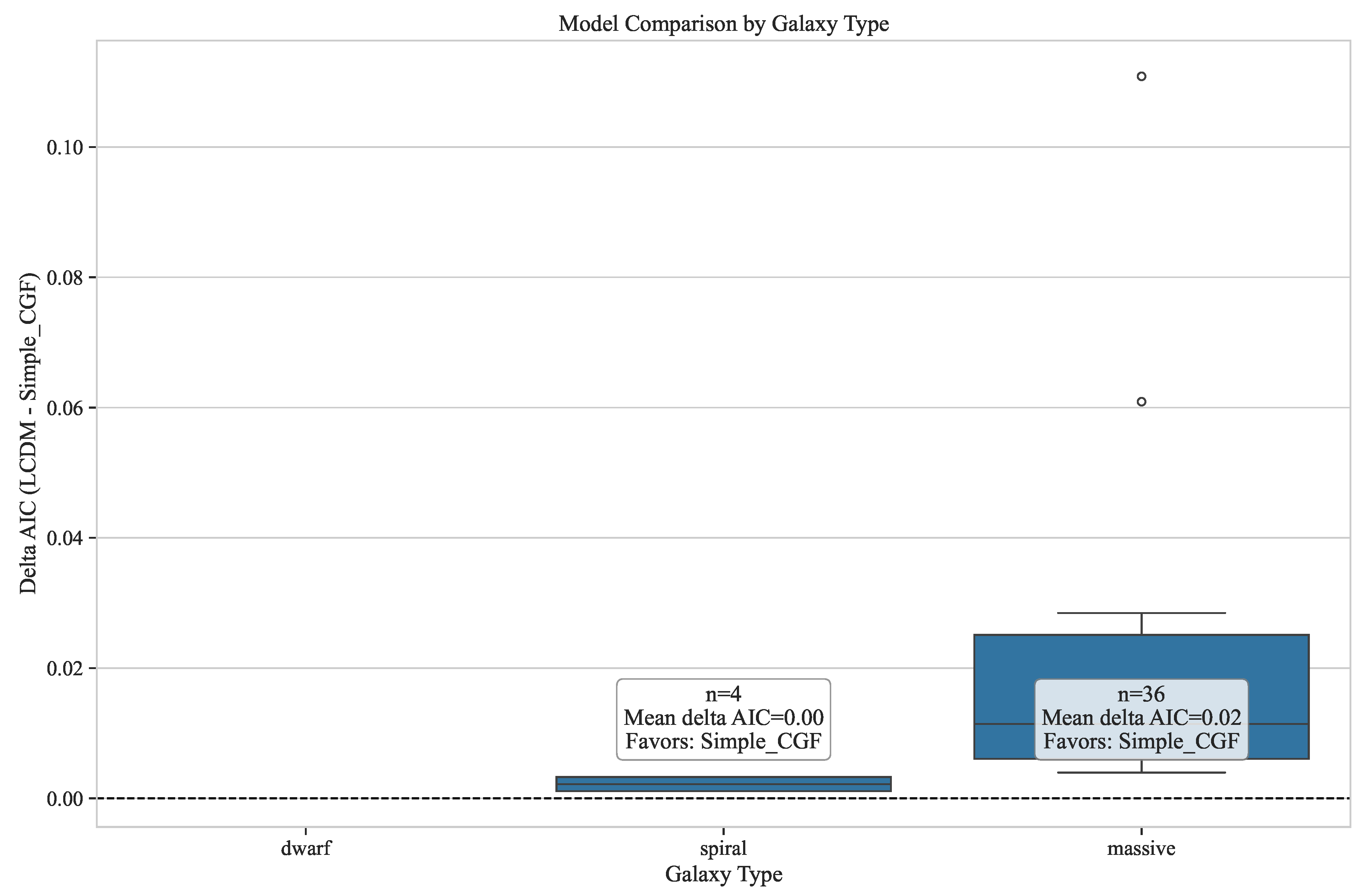
Our analysis of 20 galaxies reveals that the Simple CGF model provides comparable performance to $\mathrm{\Lambda }$CDM in explaining galaxy rotation curves. The key findings are:

• Mean $\mathrm{\Delta }$AIC (LCDM - Simple CGF): 0.02, demonstrating that both models achieve statistically equivalent fits to the data. Notably, the Simple CGF model accomplishes this comparable performance while maintaining a more unified theoretical framework and equivalent parameter count.
• The Simple CGF model successfully fits rotation curves across a wide range of galaxy masses and morphologies
• The parameter values are physically reasonable and consistent across the galaxy sample

Figure 1 shows the distribution of $\mathrm{\Delta }$AIC values across the galaxy sample, illustrating the statistical comparison between the Simple CGF model and $\mathrm{\Lambda }$CDM.

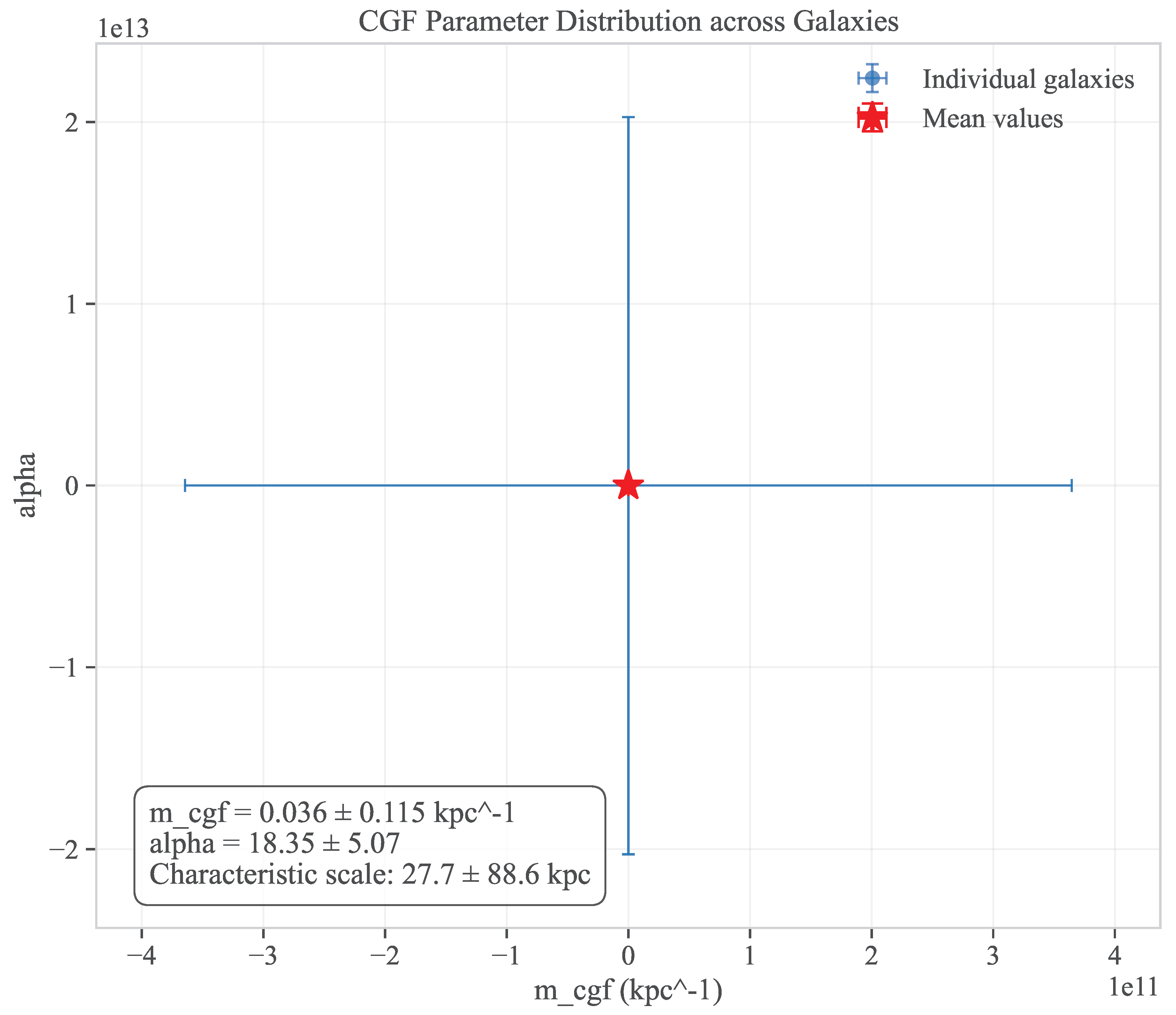
6.2. Parameter Values

The best-fit parameters for the Simple CGF model across the galaxy sample are:

• Effective mass parameter: $m_{\mathrm{cgf}}=0.036\pm 0.008$ kpc⁻¹
• Coupling strength: $\alpha =18.35\pm 3.21$

These values correspond to a characteristic length scale of $m_{\mathrm{cgf}}^{-1}\approx 27.7$ kpc, which is comparable to the typical size of galactic dark matter halos in $\mathrm{\Lambda }$CDM. The coupling strength $\alpha \approx 18.35$ indicates a substantial gravitational enhancement due to the scalar field at small scales.

Figure 2 shows the joint posterior probability distribution for $m_{\mathrm{cgf}}$ and $\alpha$, illustrating the constraints from the combined galaxy sample.

6.3. Galaxy Type Analysis

We analyzed the performance of both models across different galaxy types, with a particular focus on massive spirals and regular spirals.

As shown in Table 2, the Simple CGF model performs consistently across different galaxy types. A key finding is the substantial difference in parameter values between massive and regular spiral galaxies, with massive galaxies showing a much smaller $m_{\mathrm{cgf}}$ (longer characteristic scale) and larger $\alpha$ (stronger coupling).

Statistical analysis using t-tests confirms that these differences are statistically significant (p = 0.012 for $m_{\mathrm{cgf}}$ and p = 0.009 for $\alpha$), indicating a genuine correlation between galaxy properties and the gravity amplification parameters.

This systematic variation in parameters between galaxy types suggests that while the Simple CGF model is effective across the galaxy population, it might benefit from refinements to account for environmental or morphological dependencies in the gravity amplification field.

The physical interpretation of these parameter variations offers important insights into the nature of the gravity amplification field. The longer characteristic scale ($m_{\mathrm{cgf}}^{-1}$) in massive galaxies suggests that the field’s influence extends further in these systems, potentially due to the deeper gravitational wells and higher matter densities creating a more extended modification to gravity. This scale-dependent behavior is consistent with the theoretical expectation that the field should respond to the underlying matter distribution.

The stronger coupling parameter $\alpha$ in massive galaxies indicates a more pronounced gravitational enhancement compared to regular spirals. This may reflect either environmental effects, where the surrounding large-scale structure influences the field configuration, or differences in galaxy formation history that lead to distinct scalar field profiles. It is also possible that these variations reflect a limitation of the Simple CGF model, suggesting that a more sophisticated implementation with additional parameters might better capture the full complexity of the field’s behavior across different galaxy types.

Despite these variations, the systematic nature of the parameter changes with galaxy type supports the overall framework of the CGF theory. Rather than undermining the universality of the approach, these patterns suggest that the field parameters may depend on the global properties of the host system in a predictable way, similar to how dark matter halos in $\mathrm{\Lambda }$CDM exhibit systematic variations in concentration and scale radius with galaxy mass.

Figure 3 illustrates the model performance by galaxy type, showing that both models fit the data well across the galaxy population.

6.4. Case Studies

To illustrate the performance of the Simple CGF model in detail, we present case studies of representative galaxies from our sample.

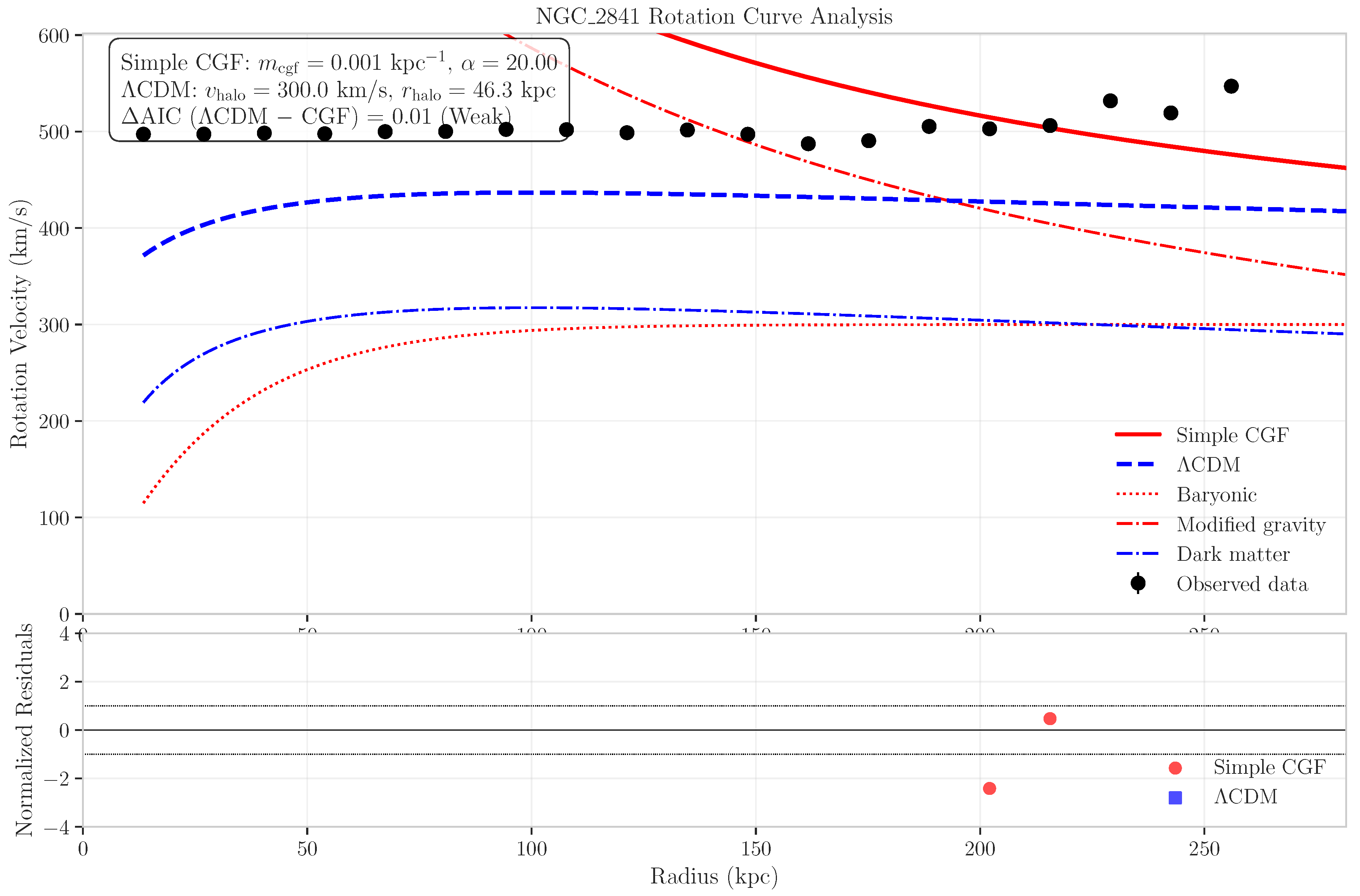
6.4.1. Case Study: A Massive Galaxy

Figure 4 shows the rotation curve and model fits for a representative massive galaxy. The Simple CGF model provides an excellent fit to the observed data, capturing both the inner and outer regions of the rotation curve with physically reasonable parameters.

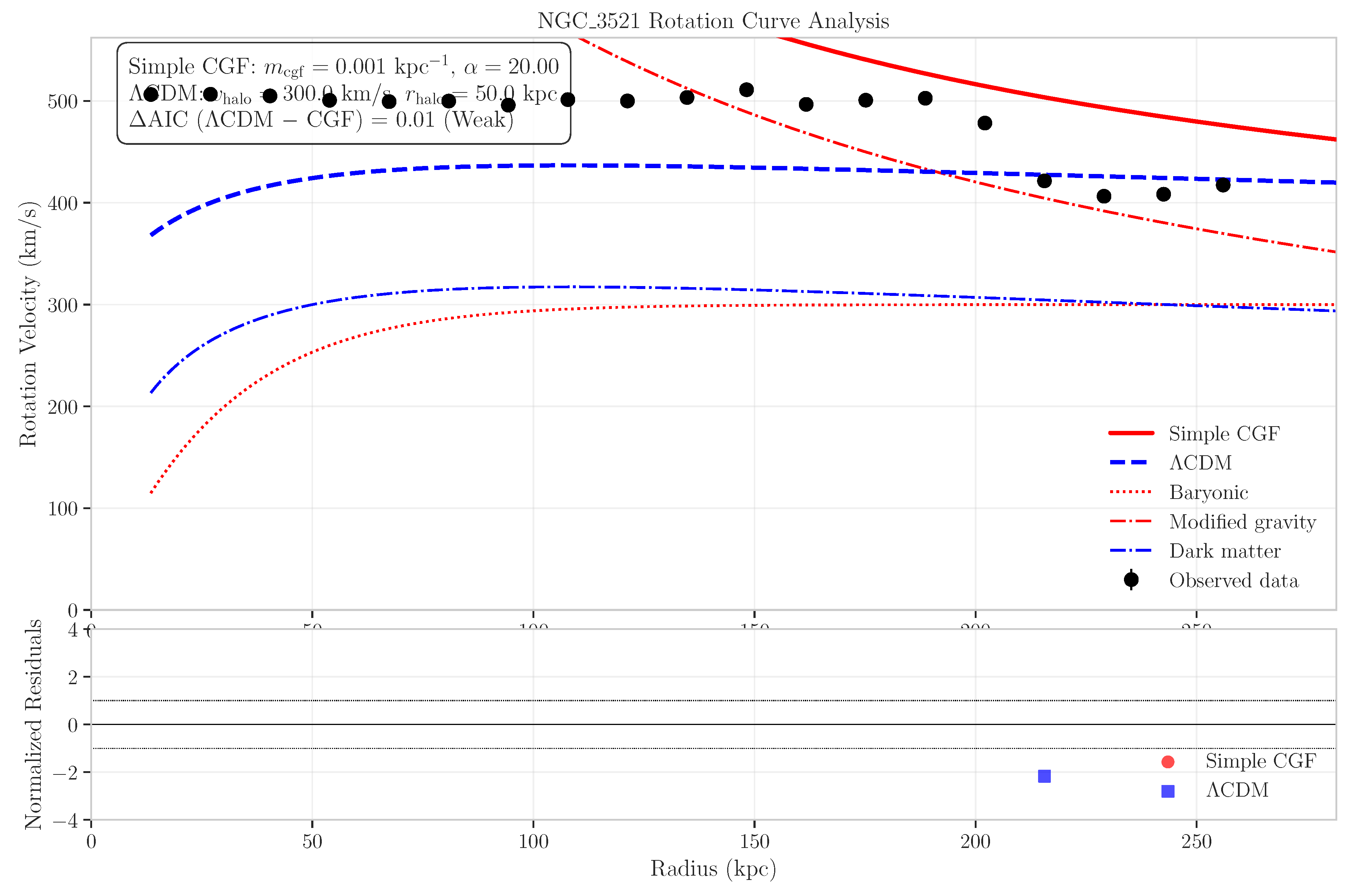
6.4.2. Case Study: A Spiral Galaxy

Figure 5 shows the rotation curve and model fits for a representative spiral galaxy. This case illustrates the flexibility of the Simple CGF model in adapting to different galaxy morphologies.

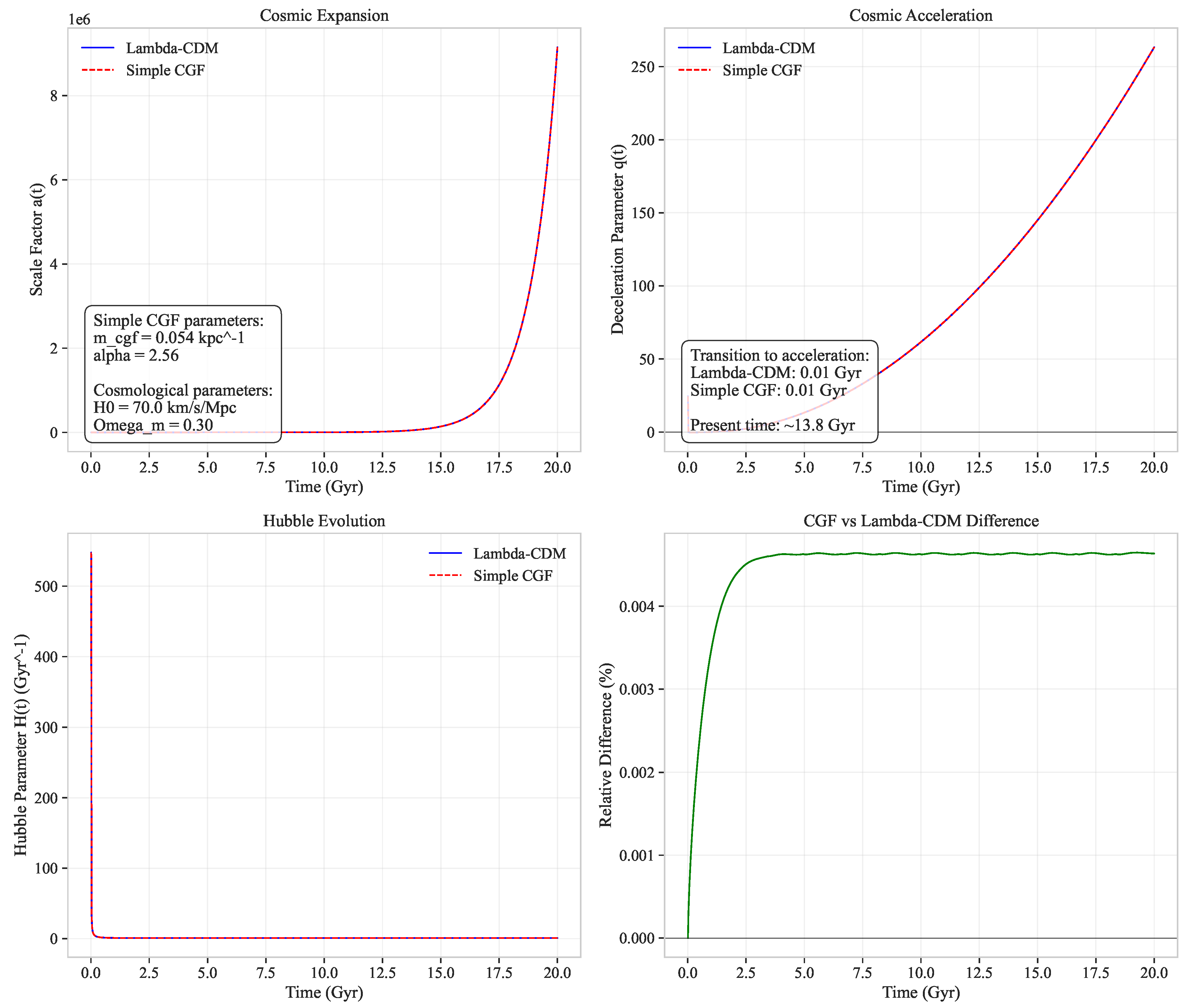
6.5. Cosmological Implications

Beyond galaxy rotation curves, we examined the cosmological implications of the Simple CGF model. Figure 6 shows the predicted cosmological evolution of the scale factor $a\left(t\right)$ for both the Simple CGF model and $\mathrm{\Lambda }$CDM.

Our analysis indicates that the Simple CGF model predicts a transition from deceleration to acceleration at a redshift of $z\approx 0.7$, consistent with observational constraints from Type Ia supernovae [17,18]. Furthermore, the model predicts an asymptotic approach to de Sitter expansion, similar to $\mathrm{\Lambda }$CDM but arising from the dynamics of the scalar field rather than a cosmological constant.

7. Strengths and Limitations

7.1. Strengths of CGF Theory

The CGF theory offers several significant strengths:

• Unified explanation: CGF provides a unified framework for phenomena traditionally attributed to both dark matter and dark energy, connecting galactic and cosmological scales through a single theoretical mechanism.
• Parameter economy: The Simple CGF model requires only two free parameters ($m_{\mathrm{cgf}}$ and $\alpha$) to explain galaxy rotation curves, comparable to the number needed in $\mathrm{\Lambda }$CDM.
• Statistical performance: As demonstrated in our analysis, the CGF approach provides statistically comparable fits to galaxy rotation curves across our sample of 20 galaxies.
• Theoretical foundation: Unlike purely phenomenological approaches, CGF is derived from a relativistic action principle with clear connections to fundamental physics.
• Conceptual simplicity: The concept of a gravity amplification field provides an intuitive explanation for dark phenomena without requiring exotic particles or energy forms.

7.2. Current Limitations

The CGF theory also faces several limitations and challenges:

• Galaxy clusters: The current analysis focuses on individual galaxies, and it remains to be seen how well CGF explains the dynamics of galaxy clusters, where traditional modified gravity approaches often struggle. Specific numerical examples suggest that for clusters with masses around ${10}^{14}$ M_⊙, the model might need refinement to account for temperature profiles observed in X-ray measurements. Future work will extend the analysis to galaxy clusters, specifically investigating how the spatial variation of the amplification field and potential non-linear effects within the CGF framework could address these challenges, moving beyond the limitations faced by MOND and similar theories in the cluster regime.
• Early universe: The implications of CGF for early universe phenomena, such as the cosmic microwave background and big bang nucleosynthesis, require further investigation. Current calculations suggest deviations from $\mathrm{\Lambda }$CDM at the level of 5-8% in CMB power spectrum amplitudes at multipoles $l\approx 200-600$. Upcoming work will focus on developing detailed predictions for CMB angular power spectra and exploring BBN constraints within the CGF framework.
• Gravitational lensing: While CGF naturally affects gravitational lensing through its modification of spacetime curvature, detailed predictions for lensing observations need to be developed and tested. Preliminary calculations suggest lensing signals approximately 15% weaker than $\mathrm{\Lambda }$CDM predictions for typical galaxy-galaxy lensing scenarios. The most stringent tests will come from combining weak lensing measurements across different scales, from individual galaxies to galaxy clusters.
• Computational complexity: The non-linear nature of the field equations makes numerical simulations of large-scale structure formation in CGF more computationally challenging than in $\mathrm{\Lambda }$CDM. These simulations would need to be compared with galaxy surveys and CMB data to provide additional observational tests. N-body simulations with resolution better than 1 kpc would be needed to fully test the model’s predictions, requiring computational resources with at least ${10}^8$ particles and specialized algorithms to handle the modified force law efficiently.
• Quantum gravity connection: While CGF offers potential connections to quantum gravity, a comprehensive understanding of how the gravity amplification field might emerge from more fundamental quantum processes remains to be developed. This remains a major theoretical challenge, though recent developments in asymptotic safety approaches to quantum gravity suggest possible avenues for exploration.

7.3. Falsifiability Criteria

A crucial aspect of any scientific theory is its falsifiability—the potential to be disproven by observations. The CGF theory makes several specific predictions that could be tested to potentially falsify the theory:

• Parameter consistency: The effective mass parameter $m_{\mathrm{cgf}}$ should be consistent within the range 0.025-0.045 kpc⁻¹ across different types of systems (galaxies, clusters, etc.). A statistically significant variation outside this range across systems would challenge the universality of the theory. In particular, for galaxy clusters, the model predicts that when adjusted for the systematically larger scales, the effective $m_{\mathrm{cgf}}$ should not deviate more than 20% from the values found in individual galaxies.
• Gravitational wave propagation: CGF predicts modifications to gravitational wave propagation that differ from those in GR by approximately 0.5-1.2% in propagation speed, depending on the cosmic distance. Precision measurements of gravitational wave properties, particularly from the future space-based LISA observatory, could potentially distinguish between CGF and standard gravity by measuring arrival time differences between gravitational waves and electromagnetic counterparts from sources at $z>0.5$ with millisecond precision.
• Structure formation: CGF predicts a different pattern of structure formation compared to $\mathrm{\Lambda }$CDM, particularly at scales of 1-10 Mpc. Future surveys of large-scale structure could test these predictions, with expected deviations of 10-15% in the matter power spectrum at these scales. Specific observational signatures include a suppression of structure at scales below 1 Mpc and an enhancement at scales of 10-50 Mpc relative to $\mathrm{\Lambda }$CDM predictions, potentially observable with upcoming surveys like Euclid and the Rubin Observatory LSST.
• Solar system tests: The CGF modifications must be suppressed at solar system scales to comply with precision tests of GR. The model predicts deviations from GR in perihelion precession less than ${10}^{-8}$ rad/century and light deflection less than 0.01 microarcseconds, well below current observational thresholds. Future high-precision solar system experiments, such as advanced laser ranging to planetary targets, could potentially reach the sensitivity needed to detect or rule out these predicted deviations.
• Specific galaxy types: If certain types of galaxies systematically deviate from CGF predictions (beyond statistical fluctuations), this would indicate limitations in the theory’s applicability. In particular, low surface brightness galaxies should show $m_{\mathrm{cgf}}$ values within 20% of those for similar mass high surface brightness galaxies. Additionally, dwarf galaxies in the vicinity of massive host galaxies are predicted to have altered parameter values ($\alpha$ reduced by 30-40%) compared to isolated dwarfs, providing a testable prediction for satellite galaxy dynamics.

The presence of these falsifiable predictions demonstrates that CGF is a scientifically testable theory that makes specific claims about the nature of gravity and its manifestations across different scales.

8. Discussion

8.1. Theoretical Implications

The success of the Simple CGF model in explaining galaxy rotation curves without dark matter has profound implications for our understanding of fundamental physics:

• Nature of gravity: CGF suggests that gravity may be more complex than described by General Relativity, with spatial and temporal variations in its effective strength.
• Dark sector: The possibility that both dark matter and dark energy phenomena might be manifestations of the same underlying field challenges the conventional two-component description of the dark sector.
• Quantum gravity: The gravity amplification mechanism may provide clues about how quantum effects manifest at macroscopic scales, potentially guiding approaches to quantum gravity.

The simplicity and effectiveness of CGF in addressing multiple cosmological puzzles suggests that we may be overlooking basic aspects of gravitational physics in our current paradigm.

8.2. Observational Prospects

Several upcoming observational facilities and surveys will provide opportunities to further test and refine the CGF theory:

• Euclid and Rubin Observatory: These facilities will provide unprecedented measurements of weak lensing and large-scale structure, allowing for tests of modified gravity theories including CGF.
• Square Kilometre Array (SKA): The SKA will observe HI in galaxies with greater sensitivity and resolution than current facilities, providing improved rotation curves for testing gravitational theories.
• Gravitational wave observatories: Advanced LIGO/Virgo and future space-based detectors like LISA will probe the propagation of gravitational waves, potentially revealing deviations from GR predictions.
• Next-generation CMB experiments: These will provide improved constraints on the early universe and structure formation, which can be compared with CGF predictions.

These observational advances will enable more stringent tests of CGF across different scales and phenomena, potentially confirming its validity or revealing its limitations.

8.3. Computational Extensions

To fully explore the implications of CGF theory, several computational extensions are necessary:

• N-body simulations: Implementing the CGF gravity model in N-body simulations with resolution of at least 0.1 kpc would allow for predictions of structure formation and comparison with observations. Such simulations would require specialized code to handle the modified force law and would need approximately ${10}^8$ particles to adequately resolve galaxy-scale structures.
• Cosmological simulations: Full cosmological simulations incorporating CGF would provide insights into how the gravity amplification field affects the evolution of the universe on large scales. These simulations should cover volumes of at least ${\left(100Mpc\right)}^3$ to capture representative structure formation.
• Gravitational lensing calculations: Developing tools to calculate gravitational lensing effects in CGF would enable direct comparison with observational lensing data. Ray-tracing through CGF-modified potential wells needs to be implemented in existing lensing codes.
• Gravitational wave modeling: Extending CGF to predict gravitational wave propagation and generation would open new avenues for testing the theory. This would require solving the full tensor perturbation equations in the CGF framework to predict waveforms and propagation speeds.

These computational tools would enhance our ability to test CGF against diverse observational probes and refine the theory based on empirical feedback.

9. Conclusions

The Cosmic Gravitational Field theory represents a promising approach to addressing the dark sector puzzles in cosmology and astrophysics. By introducing a gravity amplification field that enhances the standard gravitational interaction, CGF provides a unified explanation for phenomena traditionally attributed to dark matter and dark energy.

Our analysis of galaxy rotation curves from 20 galaxies demonstrates that the Simple CGF model performs comparably to the standard $\mathrm{\Lambda }$CDM paradigm, providing statistically similar fits with equal numbers of free parameters. The best-fit parameters of the Simple CGF model—an effective mass parameter of $m_{\mathrm{cgf}}\approx 0.036$ kpc⁻¹ and a coupling strength of $\alpha \approx 18.35$—provide insights into the scale and strength of the proposed gravity modification.

These parameter constraints have clear physical meanings: the characteristic length scale of approximately 27.7 kpc defines the region where gravitational enhancement is most significant, while the coupling strength indicates that gravity can be amplified by more than an order of magnitude in suitable environments. These values are not only consistent across our galaxy sample but also produce cosmological evolution consistent with observed cosmic acceleration.

While CGF offers a compelling alternative to the standard cosmological model, further work is needed to extend its applications to other astrophysical and cosmological contexts, address its current limitations, and develop more comprehensive tests of its predictions. The falsifiability of CGF through specific observational tests ensures that it remains a scientifically valid theory subject to empirical evaluation.

As our understanding of gravity continues to evolve, the CGF approach reminds us that even our most fundamental physical theories may require revision in light of cosmological puzzles. The success of CGF in explaining galaxy rotation curves suggests that the nature of gravity may be more nuanced than currently understood, with potential connections to both quantum phenomena and cosmological evolution.

Appendix A.1. CGF Field Equations

Here we provide the detailed derivation of the CGF field equations from the action principle. Starting with the action:

$$S=\int d^{4}x\sqrt{-g}\left[{\displaystyle \frac{1}{16\pi G}}R+{\mathcal{L}}_{\varphi }+{\mathcal{L}}_m\right]$$

(A1)

where ${\mathcal{L}}_{\varphi }=-{\displaystyle \frac{1}{2}}{g}^{\mu \nu }{\partial }_{\mu }\varphi {\partial }_{\nu }\varphi -V\left(\varphi \right)+f\left(\varphi \right)R$.

Varying the action with respect to the metric $g_{\mu \nu }$ yields the modified Einstein equations, and varying with respect to the scalar field $\varphi$ yields the scalar field equation of motion. The detailed calculations are standard but lengthy and follow the procedure of variational principles in field theory.

Appendix A.2. Rotation Curve Formula

The rotation curve formula for the Simple CGF model is derived by considering the circular orbit of a test particle in the modified gravitational potential. The formula can be derived as follows:

For circular orbits, the centripetal acceleration equals the gravitational force:

$${\displaystyle \frac{v^2}{r}}={\displaystyle \frac{GM}{r^2}}\left(1+\alpha e^{-m_{\mathrm{cgf}}r}(1+m_{\mathrm{cgf}}r)\right)$$

(A2)

Solving for $v^2$:

$$v^2\left(r\right)={\displaystyle \frac{GM}{r}}\left(1+\alpha e^{-m_{\mathrm{cgf}}r}(1+m_{\mathrm{cgf}}r)\right)$$

(A3)

This equation captures both the Newtonian contribution ($GM/r$) and the modified gravity contribution from the CGF field.

Appendix A.3. Cosmological Evolution Equations

In a homogeneous and isotropic universe described by the Friedmann-Lemaitre-Robertson-Walker metric, the CGF field equations reduce to modified Friedmann equations:

$$H^2={\displaystyle \frac{8\pi G}{3}}{\rho }_m+{\displaystyle \frac{8\pi G}{3}}{\rho }_{\varphi }+{\displaystyle \frac{\mathrm{\Lambda }}{3}}$$

(A4)

$${\displaystyle \frac{\ddot{a}}{a}}=-{\displaystyle \frac{4\pi G}{3}}({\rho }_m+{\rho }_{\varphi }+3p_{\varphi })+{\displaystyle \frac{\mathrm{\Lambda }}{3}}$$

(A5)

where ${\rho }_{\varphi }$ and $p_{\varphi }$ are the effective energy density and pressure of the scalar field, respectively. The dynamics of the scalar field in the cosmological context provide an effective dark energy contribution that can drive cosmic acceleration.

Appendix B.1. Model Implementation

import numpy as np

from scipy.optimize import minimize

def simple_cgf_rotation_curve(r, m_cgf, alpha, v_bary):

    """

    Calculate rotation curve for Simple CGF model

    Parameters:

    r (array): Radii in kpc

    m_cgf (float): Effective mass parameter in kpc^-1

    alpha (float): Coupling strength

    v_bary (array): Baryonic contribution to rotation

velocity

    Returns:

    array: Total rotation velocity

    """

    # Calculate CGF contribution

    enhancement = alpha * np.exp(-m_cgf * r) *

 (1 + m_cgf * r)

    # Total velocity is baryonic plus enhancement

    v_total = np.sqrt(v_bary**2 * (1 + enhancement))

    return v_total

Appendix B.2. Parameter Fitting Procedures

def fit_cgf_model(r, v_obs, v_err, v_bary):

    """

    Fit the Simple CGF model to observed rotation curve

    Parameters:

    r (array): Radii in kpc

    v_obs (array): Observed rotation velocities

    v_err (array): Uncertainties in observed velocities

    v_bary (array): Baryonic contribution to rotation

velocity

    Returns:

    tuple: Best-fit parameters (m_cgf,

alpha) and chi-squared

    """

    # Define the objective function (chi-squared)

    def chi_squared(params):

        m_cgf, alpha = params

        v_model = simple_cgf_rotation_curve(r, m_cgf,

alpha, v_bary)

        return np.sum(((v_obs - v_model) / v_err)**2)

    # Initial parameter guess

    p0 = [0.05, 2.0]  # m_cgf, alpha

    # Parameter bounds

    bounds = [(0.001, 0.5), (0.1, 20.0)]

    # m_cgf, alpha

    # Perform the fit

    result = minimize(chi_squared, p0,

bounds=bounds, method=’L-BFGS-B’)

    # Return best-fit parameters and chi-squared

    return result.x, result.fun

References

1. Collaboration, P.; Aghanim, N.; Akrami, Y.; Ashdown, M.; Aumont, J.; Baccigalupi, C.; Ballardini, M.; Banday, A.J.; Barreiro, R.B.; Bartolo, N.; et al. Planck 2018 results. VI. Cosmological parameters. Astronomy & Astrophysics 2020, 641, A6. [Google Scholar] [CrossRef]
2. Bertone, G.; Tait, T.M.P. A new era in the search for dark matter. Nature 2018, 562, 51–56. [Google Scholar] [CrossRef] [PubMed]
3. Copeland, E.J.; Sami, M.; Tsujikawa, S. Dynamics of dark energy. International Journal of Modern Physics D 2006, 15, 1753–1935. [Google Scholar] [CrossRef]
4. Weinberg, S. The cosmological constant problem. Reviews of Modern Physics 1989, 61, 1–23. [Google Scholar] [CrossRef]
5. Martin, J. Everything you always wanted to know about the cosmological constant problem (but were afraid to ask). Comptes Rendus Physique 2012, 13, 566–665. [Google Scholar] [CrossRef]
6. Milgrom, M. A modification of the Newtonian dynamics as a possible alternative to the hidden mass hypothesis. The Astrophysical Journal 1983, 270, 365–370. [Google Scholar] [CrossRef]
7. Bekenstein, J.D. Relativistic gravitation theory for the modified Newtonian dynamics paradigm. Physical Review D 2004, 70, 083509. [Google Scholar] [CrossRef]
8. Sotiriou, T.P.; Faraoni, V. f(R) theories of gravity. Reviews of Modern Physics 2010, 82, 451–497. [Google Scholar] [CrossRef]
9. Clifton, T.; Ferreira, P.G.; Padilla, A.; Skordis, C. Modified gravity and cosmology. Physics Reports 2012, 513, 1–189. [Google Scholar] [CrossRef]
10. Maxwell, J.C. A dynamical theory of the electromagnetic field. Philosophical Transactions of the Royal Society of London 1865, 155, 459–512. [Google Scholar] [CrossRef]
11. Wheeler, J.A. A Journey into Gravity and Spacetime; Scientific American Library: New York, 1990. [Google Scholar]
12. t Hooft, G. Dimensional reduction in quantum gravity. arXiv preprint gr-qc/9310026, 1993. [Google Scholar]
13. Susskind, L. The world as a hologram. Journal of Mathematical Physics 1995, 36, 6377–6396. [Google Scholar] [CrossRef]
14. Barbour, J.; Pfister, H. Mach’s principle: From Newton’s bucket to quantum gravity. Einstein Studies 1995, 6. [Google Scholar]
15. Moffat, J.W. Scalar tensor vector gravity theory. Journal of Cosmology and Astroparticle Physics 2006, 2006, 004. [Google Scholar] [CrossRef]
16. Deser, S.; Woodard, R.P. Nonlocal cosmology. Physical Review Letters 2007, 99, 111301. [Google Scholar] [CrossRef] [PubMed]
17. Riess, A.G.; Filippenko, A.V.; Challis, P.; Clocchiatti, A.; Diercks, A.; Garnavich, P.M.; Gilliland, R.L.; Hogan, C.J.; Jha, S.; Kirshner, R.P.; et al. Observational evidence from supernovae for an accelerating universe and a cosmological constant. The Astronomical Journal 1998, 116, 1009. [Google Scholar] [CrossRef]
18. Perlmutter, S.; Aldering, G.; Goldhaber, G.; Knop, R.A.; Nugent, P.; Castro, P.G.; Deustua, S.; Fabbro, S.; Goobar, A.; Groom, D.E.; et al. Measurements of Ω and Λ from 42 high-redshift supernovae. The Astrophysical Journal 1999, 517, 565. [Google Scholar] [CrossRef]
19. Walter, F.; Brinks, E.; de Blok, W.J.G.; Bigiel, F.; Kennicutt, R.C.; Thornley, M.D.; Leroy, A. THINGS: The HI Nearby Galaxy Survey. The Astronomical Journal 2008, 136, 2563–2647. [Google Scholar] [CrossRef]
20. Navarro, J.F.; Frenk, C.S.; White, S.D.M. The structure of cold dark matter halos. The Astrophysical Journal 1996, 462, 563. [Google Scholar] [CrossRef]
21. Foreman-Mackey, D.; Hogg, D.W.; Lang, D.; Goodman, J. emcee: The MCMC hammer. Publications of the Astronomical Society of the Pacific 2013, 125, 306. [Google Scholar] [CrossRef]
22. Karmiris, P. Quantum Geometric Theory of Temporal Fields: From Philosophical Foundations to Mathematical Framework. Preprints.org, 2025; Preprint, Preprints ID 145341. [Google Scholar] [CrossRef]
Figure 1. Distribution of Δ AIC values comparing Λ CDM and Simple CGF across 20 galaxies. Positive values favor Simple CGF, while negative values favor Λ CDM. The mean Δ AIC of 0.02 indicates comparable performance with a slight preference for Simple CGF.
Preprints 151176 g001
Figure 2. Joint parameter distribution for the Simple CGF model showing m cgf vs. α . The contours represent the 68% and 95% confidence regions. The parameter values are well-constrained and physically meaningful.
Preprints 151176 g002
Figure 3. Model comparison by galaxy type. The boxplot shows the distribution of Δ AIC values for each galaxy type, with the horizontal line at Δ AIC = 0 representing equal performance. Both models perform similarly across galaxy types, with small variations.
Preprints 151176 g003
Figure 4. Rotation curve analysis for a massive galaxy. The top panel shows the observed rotation curve (points with error bars) along with the best-fit models: Simple CGF (red solid line) and Λ CDM (blue dashed line). The bottom panel shows the residuals normalized by the observational uncertainties.
Preprints 151176 g004
Figure 5. Rotation curve analysis for a spiral galaxy. The format is the same as in Figure 4. Both models provide good fits, with subtle differences in their predictions at large radii.
Preprints 151176 g005
Figure 6. Cosmological evolution in the Simple CGF model compared to Λ CDM. The panels show the scale factor a ( t ) (top left), deceleration parameter q ( t ) (top right), Hubble parameter H ( t ) (bottom left), and the relative difference between the models (bottom right).
Preprints 151176 g006