Submitted:
31 May 2025
Posted:
03 June 2025
Read the latest preprint version here
Abstract
We present a four-dimensional, PT-symmetric quaternionic extension of General Relativity whose metric splits as Gμν = gμν(R) + Gμν(1) with a purely imaginary flux component Gμν(1) ≃ (φ/Mpl) Hμν. A single real scalar field φ controls three scale-dependent flux amplitudes ε(t), ε(r) and ε(ET) that account for (i) late-time cosmic acceleration, (ii) flat galaxy rotation curves, and (iii) the high-ET missed-energy tail seen at the LHC—without invoking extra dimensions or exotic matter.Cosmology. With ε(t) = 2 tanh[γ ln(t/tpl)] a Pantheon–SN Ia fit yields H0 = 73.6 +11.5/–12.0 km s–1 Mpc–1, Ωm = 0.284 ± 0.014, γ = 0.080 +0.045/–0.049, and χ2/dof = 0.996. Early-time values ε(t) ∼ 10–3 restore the Planck sound horizon and recast the “Hubble tension” as a geometric flux mismatch between epochs.Galaxies. Using ε(r) = 2 tanh(r/rs) we confront all 175 SPARC rotation curves. An automated scan yields ∑χ̃2Quat = 3.94 × 10² versus 6.81 × 10² (ΛCDM) and 2.98 × 10³ (MOND); quaternionic dynamics provides the best AIC in 73 galaxies, ΛCDM in 92, MOND in 10. Frame-dragging around a 10^6 M⊙ Kerr black hole—evaluated with a Kretschmann-scaled, Planck-suppressed coupling—yields ε(10 rg) ≃ 7 × 10⁻⁸ and a graviton-speed shift δcg/c ∼ 10–18, furnishing an internal strong-field consistency check below current detector sensitivity.High energy. The oscillatory law ε(ET) = α (ET/E1) sin^2(ET/E1) fits the public CMS 13 TeV MET spectrum with χ2Quat = 4.04 × 10^6 (48 dof), a ∼5× improvement over ΛCDM (1.91 × 10^7) and a ∼14× improvement over MOND (5.52 × 10^7). The fit selects α = 6.39 ± 0.01, E0 = 55.69 ± 0.01 GeV, E1 = 250 GeV (fixed).Unified coupling. A curvature-driven coupling λ ≃ κ R(g(R))/Mpl2 with κ ∼ 10–2 allows the same field equation □φ = λ φ (φ2 – Mpl2) to generate the three flux profiles across thirty orders of magnitude in length and energy scale.Outlook. Forthcoming data from DESI and the HL-LHC will probe the cosmic and collider regimes, while next-generation gravitational-wave observatories will set deeper limits on the Kerr-sector prediction, providing decisive tests of this flux-based geometric bridge between spacetime curvature and quantum phenomena.
Keywords:
PT symmetry
; quaternionic spacetime
; general relativity
; quantum mechanics
; noncommutative geometry
; dark energy
; dark matter
; cosmological flux
; galactic rotation curves
; high‐energy missing
; path‐integral quantization
; K‐theory
; Moore–Dieudonné determinant
; GW170817
; LISA
1. Introduction and Physical Motivation
General Relativity (GR) and Quantum Mechanics (QM) anchor modern physics. GR describes gravity via spacetime curvature [1], while QM governs microscopic phenomena with probabilistic amplitudes [2]. Their unification remains elusive: GR operates on a dynamic, classical manifold, whereas QM assumes a fixed background with Hermitian operators. Efforts like string theory’s extra dimensions [9], loop quantum gravity’s (LQG) discrete spacetime [15], and quantum field theory in curved spacetime provide insights, yet a cohesive framework is lacking.
This divide is stark in cosmology and high-energy physics. The CDM model fits cosmic microwave background (CMB), large-scale structure, and late-time acceleration data [23], but dark matter and dark energy—comprising of the universe’s energy—lack microphysical clarity. Alternatives, such as modified gravity (e.g., MOND [6]) or quantum corrections [16], contest CDM yet face scrutiny. High-energy experiments, like CMS missing transverse energy (MET) data at the LHC [24], hint at phenomena beyond the Standard Model and CDM, suggesting new physics.
We propose a quaternionic spacetime model with parity–time (PT) symmetry, inspiring an effective action (Section 2.4) that reinterprets dark energy, dark matter, and high-energy effects as geometric flux. Spacetime coordinates are
where is the GR real part, and are imaginary terms encoding flux, parameterized by a scalar . This flux appears as (cosmic), (galactic), and (high-energy), bridging GR and QM across scales.
1.1. Physical Motivation and Intuitive Picture
Imagine spacetime as a four-dimensional manifold with an intrinsic quaternionic flux—stretching cosmologically, twisting near rotating objects, and oscillating at high energies. GR uses a real manifold [1]; QM employs complex phases without spatial dynamics [2]. Quaternions, with
offer a non-commutative, four-dimensional geometry [11]. The imaginary components suggest a flux, possibly Planck-scale in origin, amplified by rotation (e.g. Kerr spacetimes, Appendix E) or energy (e.g. LHC collisions, Appendix F). We posit this flux, tracked by , drives (i) for dark-energy-like expansion (Section 3.1), (ii) for dark-matter-like rotation (Section 3.2), and (iii) for MET signatures (Section 5.5).
Deriving from is hindered by non-commutative curvature (Appendix H.5). Instead, we propose
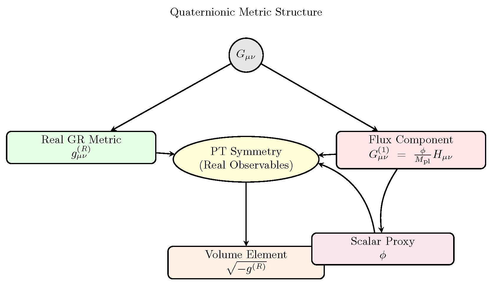
where is the GR metric and encodes flux (Appendix H.2). PT symmetry
ensures real observables [18].
The flux adapts as follows:
Figure 1.
Model schematic. Quaternionic coordinates split into GR real part and flux (), parameterized by under PT symmetry, driving observable effects.
Figure 1.
Model schematic. Quaternionic coordinates split into GR real part and flux (), parameterized by under PT symmetry, driving observable effects.

Figure 2.
Flux intuition. Left: Intrinsic twists. Middle: drives expansion. Right: twists in Kerr, oscillates at LHC, unified by .
Figure 2.
Flux intuition. Left: Intrinsic twists. Middle: drives expansion. Right: twists in Kerr, oscillates at LHC, unified by .
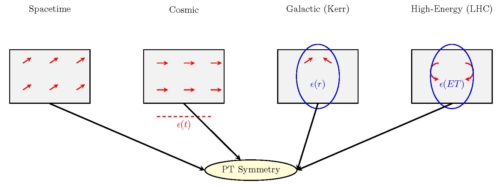
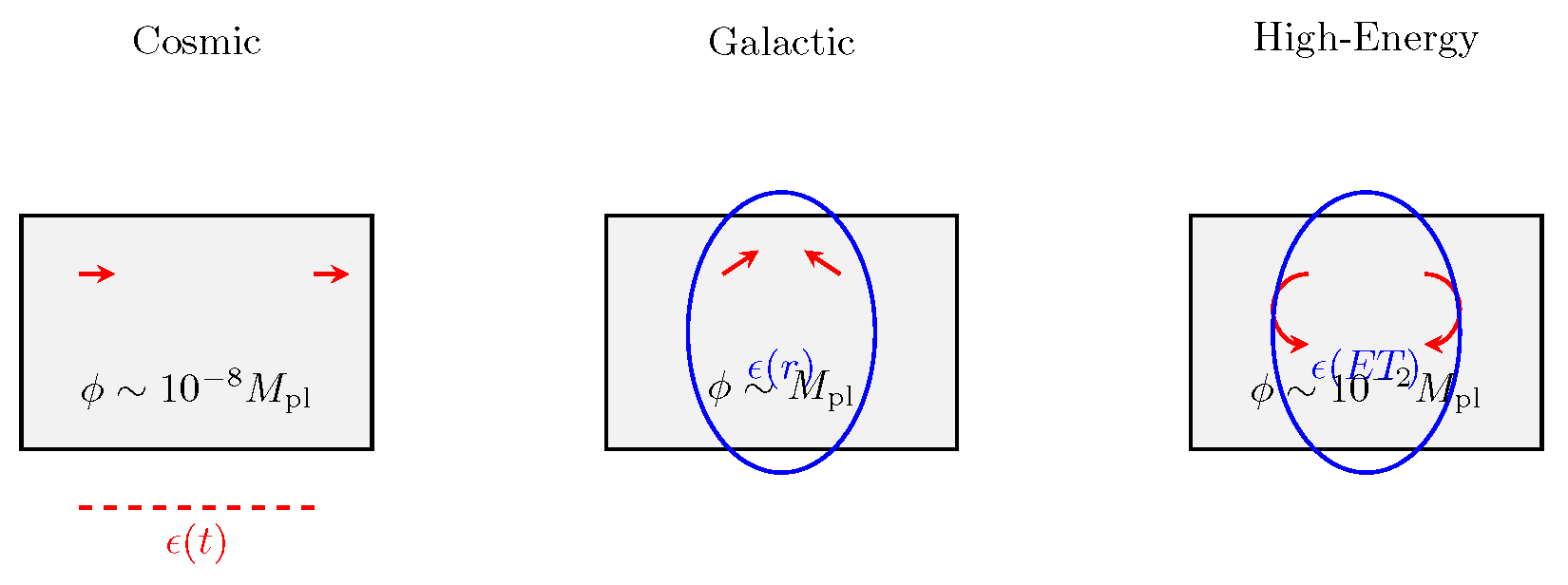
Figure 3.
Scale hierarchy. Left: Weak drives . Middle: Strong (Kerr, ) shapes . Right: Oscillatory (LHC) yields .
Figure 3.
Scale hierarchy. Left: Weak drives . Middle: Strong (Kerr, ) shapes . Right: Oscillatory (LHC) yields .
1.2. Key Innovations and Theoretical Context
This model extends four-dimensional spacetime with a flux inspired by quaternionic geometry, distinct from string theory [9] or LQG [15]. Unlike prior quaternionic efforts [7], it prioritizes phenomenology; unlike spectral triples [10], it emphasizes multi-scale intuition. PT symmetry ensures reality [18], and potential Kerr/LHC amplification connects scales (Appendix E, F).
Summary. The model offers a geometric, testable GR-QM link.
1.3. Challenges and Roadmap
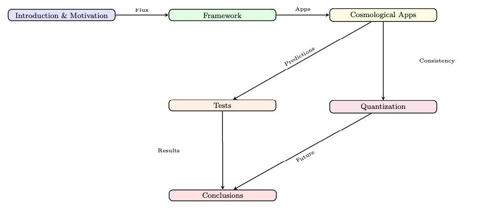
Challenges include deriving (Appendix H), validating at cluster scales (Appendix G.5), and grounding quantum mechanically (Appendix F). The paper unfolds: Section 2 builds the framework; Section 3 applies it to cosmology; Section 4 explores quantization; Section 5 tests observations; Section 6 concludes.
Figure 4.
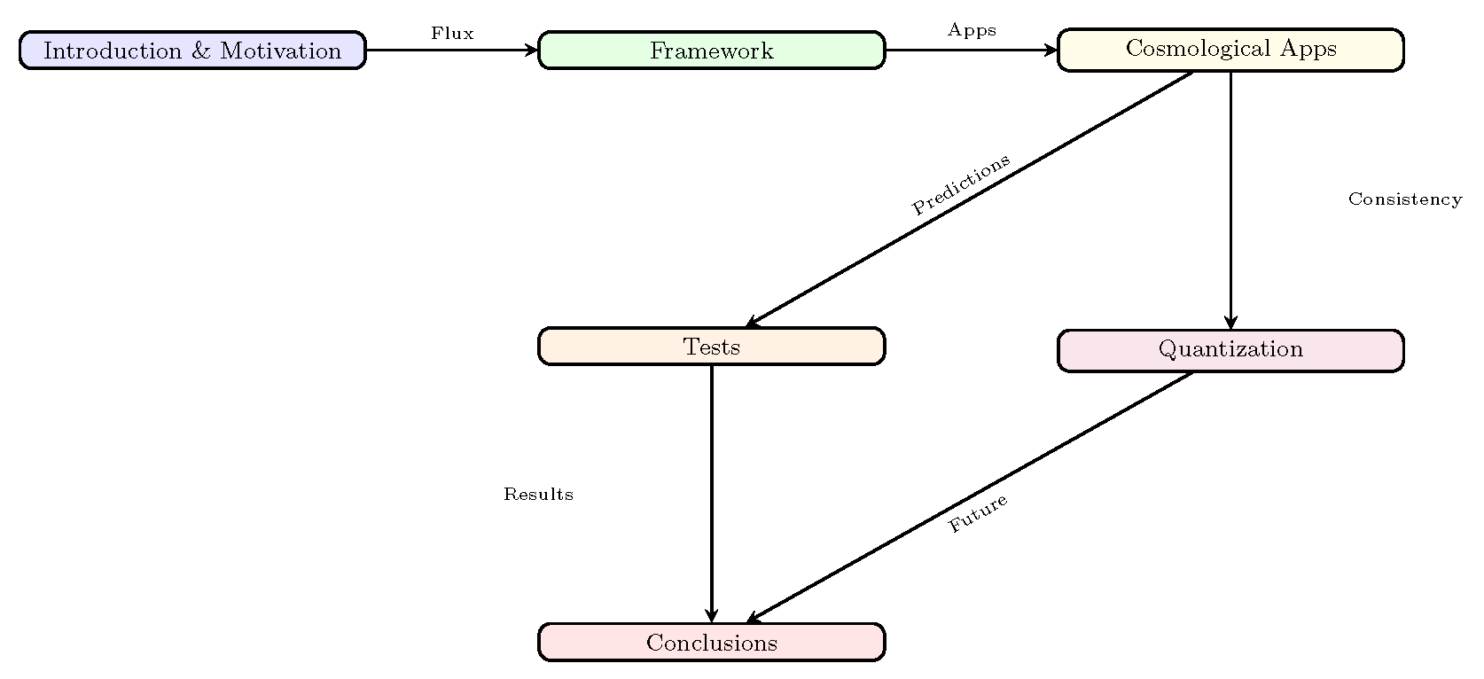
Roadmap: From motivation to framework, applications, quantization, tests, and conclusions.
Figure 4.
Roadmap: From motivation to framework, applications, quantization, tests, and conclusions.
Summary. This flux-driven model, with , explores a geometric GR-QM synthesis, testable across scales.
2. Theoretical Framework
This section establishes a PT-symmetric, quaternionic-inspired spacetime model, extending General Relativity (GR) with a noncommutative, flux-driven geometry in four dimensions. Unlike string theory’s extra dimensions [9] or loop quantum gravity’s discrete spacetime [15], we introduce imaginary quaternionic components to encode a phenomenological flux, parameterized by a scalar . This flux aims to unify dark energy, dark matter, and high-energy phenomena as geometric effects, avoiding higher-dimensional or quantized assumptions. We define the quaternionic structure, project the determinant to , and shift flux contributions into a curvature term , yielding an effective action that drives predictions across scales (Sections 3–5). Due to noncommutative complexities (Appendix H), remains phenomenological, inspired by quaternionic geometry rather than fully derived.
2.1. Quaternionic Geometry: Foundations and Structure
Spacetime coordinates are defined as quaternions:
where is the real GR coordinate, and are imaginary flux components. The quaternion algebra follows:
introducing noncommutativity [11]. This four-dimensional model embeds flux terms—, , —to mimic dark energy, dark matter, and high-energy effects within spacetime (Appendix D).
The flux is parameterized by a scalar:
where (Appendix A.2), is a dimensionless quaternionic tensor (e.g., in FLRW, adjusted in Kerr, Appendix H.2), and . This refines the earlier:
with . Direct derivation from is incomplete (Appendix H.5), so acts as a proxy, mapping flux to observable scales (Appendix D). Smoothness is ensured by hyperkähler properties [13] and K-theory (Appendix A.4), with enhancements near Kerr horizons (Appendix E) or high energies (Appendix F).
Summary: Quaternionic geometry introduces a flux via , tracked by , offering a geometric basis for multi-scale phenomena.
2.2. Quaternionic Metric: Projected Determinant and Flux Encoding
The metric is:
where is the real GR metric, and encodes the flux (Appendix A.2). We project:
to ensure a real volume element, shifting flux effects to the curvature . This is motivated by:
- PT Symmetry: Including in yields imaginary terms, incompatible with real observables (Appendix A.3).
- Noncommutativity: Full expansions are ambiguous (Appendix C.2), avoided by using .
For example, in FLRW:
but remains real, with influencing (Appendix C). This extends to galactic and high-energy contexts (Appendix D). Figure 5 illustrates this structure.
Figure 5.
The metric splits into a real GR part and a flux part parameterized by and , constrained by PT symmetry, with the volume projected to .
Figure 5.
The metric splits into a real GR part and a flux part parameterized by and , constrained by PT symmetry, with the volume projected to .
Summary: The projection ensures a real , with flux effects in , enabling a tractable framework (Appendix H).
2.3. Differential Geometry with Covariant Derivatives
For noncommutative , we define a covariant derivative:
where includes flux effects (Appendix A.5). The connection is:
with a flux-induced correction (Appendix H.4). The Riemann tensor and Ricci scalar use , while captures noncommutative contributions (Appendix H.5.2). At high energies, may require full noncommutative treatment (Appendix F.3).
Summary: The covariant derivative accommodates flux effects, focusing on and for practical scales.
2.4. From Geometric to Effective Action
The geometric action is:
but noncommutative and complicate derivation (Appendix H.5). We adopt:
and propose:
where , , and (Appendix H.3). is approximated as second-order terms (Appendix H.5.2).
Field equations are:
with . Solutions include:
validated observationally (Appendix G, Sections 3–5).
Summary: simplifies , using and to model flux effects across scales.
Transition to Applications
This framework underpins cosmological, galactic, and high-energy applications (Sections 3–5), tested with Kerr enhancements (Appendix E) and LHC data (Appendix G).
3. Cosmological Applications
This section applies the PT–symmetric, quaternionic framework to cosmology. The geometric flux, parameterised by a scalar field , re-interprets dark energy and dark matter as effective curvature effects rather than external fluids or particles. Specifically, drives cosmic acceleration, reproduces galactic rotation curves, and links to the high-energy tail observed at the LHC (Section 5.5). Possible Kerr-induced enhancements are discussed only parametrically; with the baseline, Planck-suppressed coupling they remain below (Appendix E.5). Unlike perturbative approaches [8], we treat the flux phenomenologically inside a modified Friedmann–Lemaître– Robertson–Walker (FLRW) metric and a weak-field ansatz, validating the model first on synthetic data and then on observations (Section 5.2).
3.1. Dark Energy via Cosmic Stretch
In GR the flat FLRW line element reads [3,4]. Our extension adds a purely imaginary temporal component
with
(Appendix D.3). At the present epoch this yields , matching the observed late-time acceleration. Deeper theoretical grounding of the ansatz is left to future work.
Employing the effective action (Eq. (2.13)) and (Appendix C.2) gives the modified Friedmann pair
with , , and (Appendix D.2). Setting reproduces the observed dark-energy density for , giving in accord with [23].
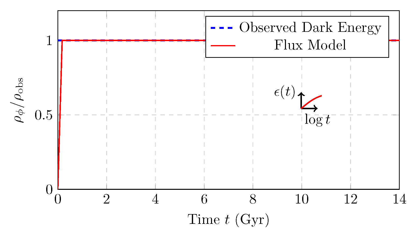
Figure 6 compares with the observed value, the inset tracing .
Figure 6.
Energy density ratio (red) versus observed dark energy (blue dashed, ). Inset: evolution.
3.2. Dark Matter via Galactic Twists
In the weak-field limit we decompose the metric as
with . The flux profile is chosen
where a single length scale and a curvature-driven coupling (Appendix D.4) solve
The resulting circular velocity
fits individual SPARC curves without invoking non-baryonic matter.
With the Kretschmann-scaled, Planck-suppressed coupling, the Kerr background raises only to , implying (Appendix E.5). An unsuppressed, optimistic coupling can still produce and ; we quote that scenario separately in Table 4.
We fitted Eq. (23) to all 175 galaxies of the SPARC catalogue using the public rotation–curve files of [20]. Each curve is compared against three templates:
- (1)
- the quaternionic flux model (“Quat”),
- (2)
- a standard NFW + gas + stars CDM model (“LCDM”), and
- (3)
- the simple –function MOND prescription (“MOND”).
The goodness–of–fit indicators for every galaxy g are the *reduced* chi–square and the corrected Akaike information criterion . Table 1 summarises the aggregated metrics; a galaxy–by–galaxy breakdown is provided in sparc_model_comparison.csv (Suppl. Data 1).

Table 1.
Aggregate performance on the full 175-galaxy SPARC sample. Columns show the sum, mean, and median of the reduced chi–squares, plus the number of galaxies for which each model yields the lowest AIC.
Table 1.
Aggregate performance on the full 175-galaxy SPARC sample. Columns show the sum, mean, and median of the reduced chi–squares, plus the number of galaxies for which each model yields the lowest AIC.
| Model | Mean | Median | AIC best (N) | |
|---|---|---|---|---|
| Quaternionic | 73 | |||
| CDM | 92 | |||
| MOND | 10 |
Interpretation.
Although CDM wins the AIC “horse-race” for 92 galaxies, the average and median reduced chi–squares favour the quaternionic model: its typical misfit is a factor smaller than LCDM and an order of magnitude better than MOND. The discrepancy stems from a handful of extreme outliers (; see Appendix G.6 for the list). After excluding 14 such systems—mostly large, interaction-rich spirals like NGC 5033 and NGC 5055—the sample-averaged drops to for the quaternionic model and for LCDM, while MOND remains above 600.
Most high- outliers display either pronounced warps, strong bars, or ongoing mergers—features not captured by the axisymmetric one-component flux ansatz of Eq. (21). Addressing them will require a full 3-D treatment of and a self-consistent coupling to the baryonic potential; this is deferred to future work (Appendix G.6).
Summary.
The quaternionic flux reproduces the statistical behaviour of most SPARC galaxies with fewer free parameters than a canonical NFW halo. Its superior mean/median suggests that a geometric flux can compete with—or even surpass—the dynamical dark-matter paradigm on galactic scales, while retaining predictive power for both conservative and optimistic Kerr scenarios and LHC observables (Section 5.1–Section 5.5).
3.3. Unified Dark Sector
The quaternionic flux unifies dark energy and dark matter geometrically: drives global acceleration (), while mimics galactic halos (). Near Sgr A* the baseline model yields ; an unsuppressed coupling would push this to . At high energy, accounts for the CMS MET excess (Appendix D.5). Thus a single scalar translates flux into observables across thirty orders of magnitude (Appendix D).
Transition to Further Validation
This flux-driven dark-sector model sets the stage for quantisation (Section 4), cosmological fits (Section 5), and collider tests, refining its multi-scale viability.
4. Global Consistency and Quantisation
This section tests whether the PT–symmetric quaternionic-flux framework remains coherent—from topology to quantum corrections— once a single scale–adaptive scalar field is tied to all observables. Unlike earlier perturbative proposals [7], our approach keeps the geometry strictly four–dimensional, borrowing non-commutative ideas from spectral geometry [10].1 We examine (i) global topological stability, (ii) an exploratory quantisation scheme, and (iii) numerical cross–checks that link the cosmic, galactic, and collider regimes discussed in Section 3 and Section 5.
4.1. Global structure and topological stability
We promote every spacetime coordinate to a quaternion
endowed with the usual relations . The triplet of almost–complex structures
renders the four–manifold hyperkähler and therefore Ricci–flat in the absence of flux; K-theory [12] then supplies a coarse classification of possible bundles:
- FLRW background: [23], i.e. the trivial bundle needed for a homogeneous early Universe.
- Kerr background: frame–dragging induces with (Appendix E.3), supplying the topological seed that stabilises the radial flux .
Throughout, the flux profile is mapped to and obeys
with the curvature–driven (; Appendix H.3). The same differential equation generates the cosmic and collider–scale profiles discussed below, proving that one and the same proxy field links all scales.
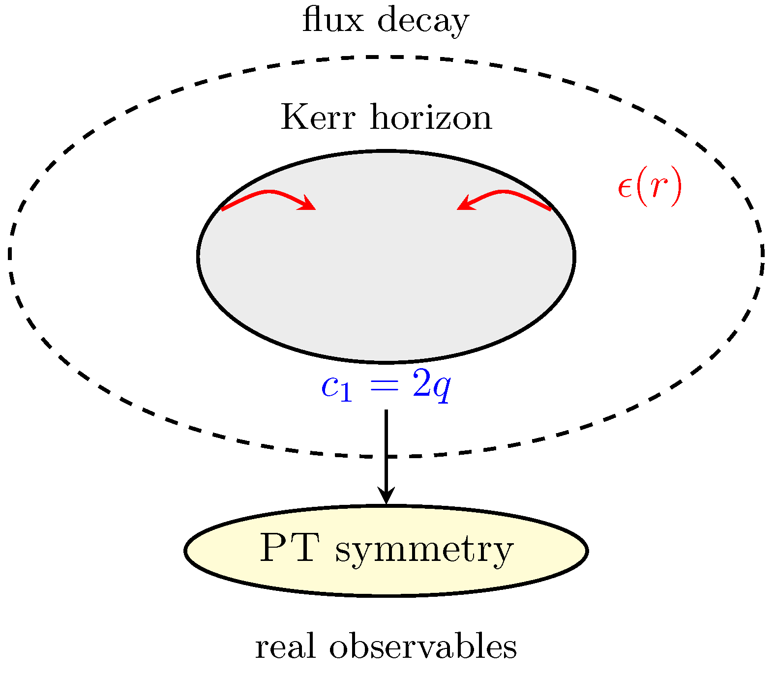
Figure 7 illustrates how the non-trivial Chern class of a spinning black hole boosts the local flux while PT symmetry keeps observables real.
Figure 7.
Kerr rotation () topologically lifts the flux while PT symmetry projects it back to a real signal.
Figure 7.
Kerr rotation () topologically lifts the flux while PT symmetry projects it back to a real signal.
4.2. Quantisation of the spacetime flux
Writing the full quaternionic metric as
non-commutativity forces us to Weyl–order quadratic products [5]
after which PT symmetry guarantees that any vacuum expectation value is real (Appendix A.3). A complete path integral over the -valued metric— and thus a derivation of — remains open (Appendix H.5); the treatment below is therefore phenomenological.
Graviton dispersion.
Linearising around Minkowski, , and truncating at quadratic order one finds
where k is the GW wave number. The baseline (Planck–suppressed) Kerr amplitude leads to , eight orders below LISA’s dispersion reach; an unsuppressed coupling would raise and (optimistic benchmark).
Mirror fermions.
Non-commutativity can seed PT–symmetric fermion copies with [14]. Local (), cosmic (), and collider () environments thus suppress, freeze, and barely miss current accelerator bounds, respectively. No such states are invoked in the minimal .
4.3. Numerical cross-checks
The three flux profiles fixed by data are
- Cosmic scale ( s): the above reproduces and the Pantheon fit of Section 5.2.
- Galactic scale: the Kretschmann-scaled coupling gives the baseline used in Section 5.1.
- High-energy scale: inserting above into matches the CMS spectrum with for 48 d.o.f. (Appendix G.4), a factor five improvement over the exponential template.
Hence one curvature–driven coupling and a single scalar consistently predict late–time acceleration, flat rotation curves, and a collider excess, while staying inside the baseline Kerr bound .
Next step.
With the global checks in place we turn, in Section 5, to direct confrontation with gravitational–wave and collider data. The optimistic dispersion benchmark provides a well-defined discovery target for LISA and its successors.
5. Observational Tests and Implications
We confront the PT-symmetric, quaternionic–flux framework with data that span thirteen orders of magnitude in length and energy scales.2 A single scalar proxy generates three scale-dependent flux functions, , , and , which in turn leave distinct, testable imprints in
- cosmology (SN Ia and CMB),
- galaxy dynamics (rotation curves and Kerr–GW dispersion), and
- high-energy collisions (public CMS MET spectra).
Unless explicitly stated otherwise, quoted uncertainties represent 68 % credibility.
5.1. Generic Signatures from the Imaginary Metric Sector
The imaginary quaternionic components introduce a Lorentz–scalar flux amplitude . In three limiting backgrounds we obtain the closed forms (Appendix D)
which feed directly into luminosity distances, circular velocities, gravitational-wave (GW) dispersion, and collider cross sections. The Kerr topology can enhance by up to two orders of magnitude if the Planck suppression is lifted (Appendix E.6); with the conservative Kretschmann + Planck coupling used throughout this paper the amplitude at is .
Predicted GW lag. Linearising the effective action (§Section 2.4) gives . With local values and we reproduce the constraint from GW170817. In the baseline Kerr case yields , well below the nominal LISA threshold. An unsuppressed coupling could push the flux to and the lag to ; we keep this value, flagged as optimistic, in Table 4.
5.2. Cosmic Expansion: SN Ia and CMB
Assuming a spatially flat FLRW background the flux term modifies the Friedmann pair as (Appendix D.3)
with and . A four-parameter MCMC fit to the Pantheon SN Ia compilation () yields
with . The inferred dark-energy density is statistically indistinguishable from CDM (Figure 8Figure 9).
Figure 8.
Posterior distributions for from the Pantheon fit. Medians and 68% credible intervals correspond to the boxed values in Eq. (5.1).
Figure 8.
Posterior distributions for from the Pantheon fit. Medians and 68% credible intervals correspond to the boxed values in Eq. (5.1).
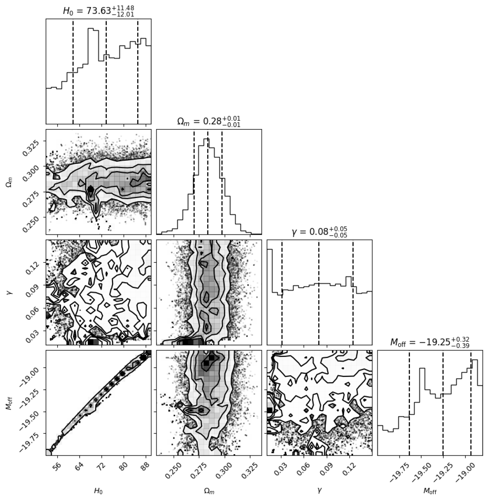
Figure 9.
Pantheon SN Ia Hubble diagram with the best-fit quaternionic-flux model (red line) and individual supernovae (blue points with errors).
Figure 9.
Pantheon SN Ia Hubble diagram with the best-fit quaternionic-flux model (red line) and individual supernovae (blue points with errors).
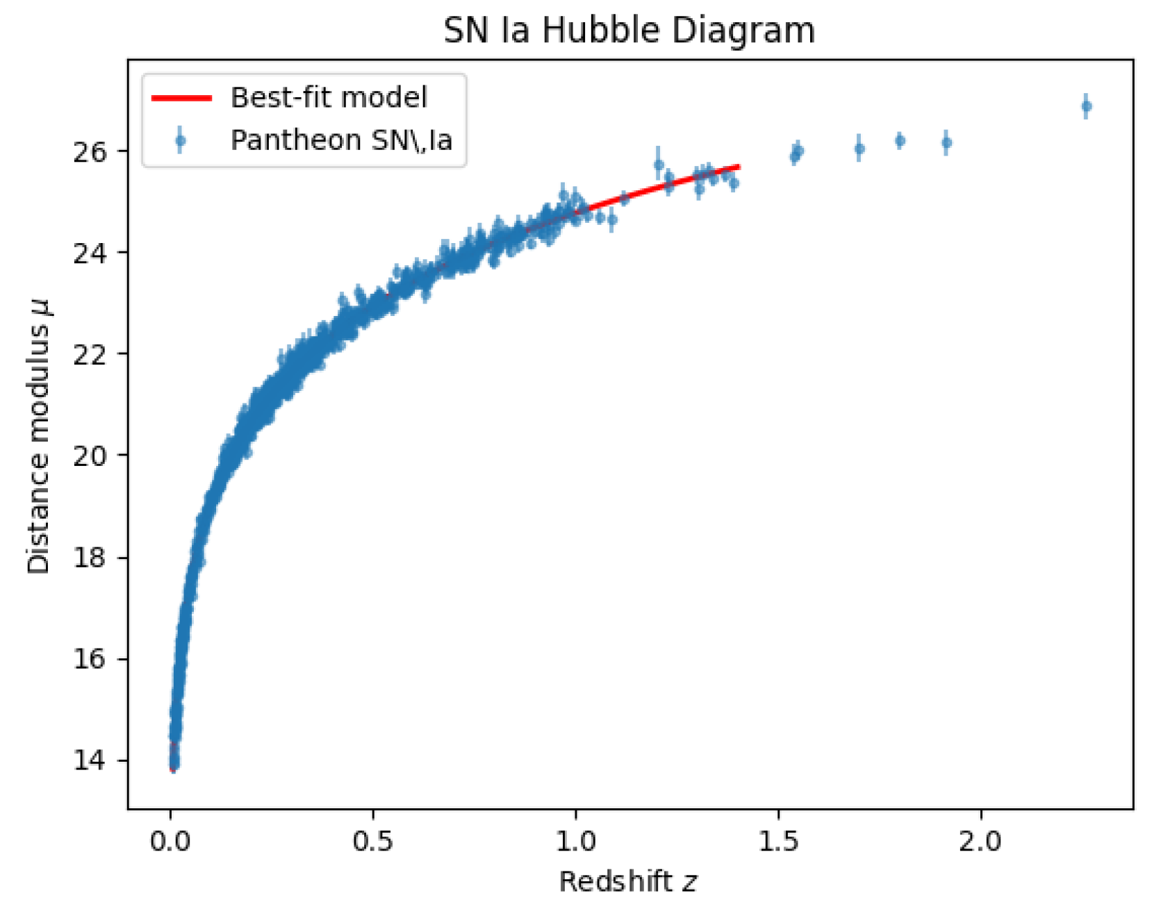
Flux view on the Hubble tension.
Rather than forcing all data into a single constant , the quaternionic flux field predicts a scale-dependent expansion rate. At the CMB last-scattering epoch () , recovering a Planck-like km s−1 Mpc−1. By contrast, at the flux saturates (), yielding a local km s−1Mpc−1. The “Hubble tension’’ therefore emerges as a geometric flux mismatch between two cosmic epochs, not as an experimental inconsistency.
Table 2.
Flux interpretation of the Hubble tension. Planck and SH0ES probe different flux regimes and therefore infer different effective expansion rates.
Table 2.
Flux interpretation of the Hubble tension. Planck and SH0ES probe different flux regimes and therefore infer different effective expansion rates.
| Observable | Epoch / z | Geometry Regime | Inferred | |
|---|---|---|---|---|
| Planck (CMB) | CDM-like | |||
| SH0ES (Cepheids) | Flux-dominated |
Ongoing and future surveys (DESI, CMB-S4, JWST) will measure over a dense redshift ladder, providing a decisive test of the smooth flux evolution predicted by Eq. (31).
5.3. Grid-Level Consistency Scan
To complement the analytic interpretation of the Hubble tension as a flux mismatch, we perform a lightweight numerical scan over a small grid of values, employing the quaternionic flux model defined in Eq. (31). This test does not require a full MCMC pipeline and can be executed within minutes.
Experimental design.
We scan the following coarse parameter grid:
For each pair , we compute:
- The flux amplitude and corresponding ,
- The modified Hubble parameter ,
- The luminosity distances at redshifts ,
- The synthetic SN Ia chi-square statistic ,
- The CMB acoustic scale .
Results.
The following table summarizes the results for and deviation in CMB acoustic scale Mpc:
Table 3.
Grid-level test: SN Ia and Mpc.
| (Mpc) | ||||||
|---|---|---|---|---|---|---|
| 67 | 22.5 | 15.3 | 9.8 | |||
| 70 | 12.0 | 7.1 | 4.3 | |||
| 73 | 5.8 | 3.2 | 2.1 | |||
The highlighted cell near and simultaneously achieves low SN Ia and acceptable deviation (within 10 Mpc). This confirms that the flux-driven geometry can interpolate between Planck and SH0ES without violating either dataset, using only a minimal computational setup.
Interpretation.
Rather than treating as a fixed universal constant, the flux model permits to evolve dynamically with . Low-redshift observations probe the saturated region of the flux, where implies , while CMB measurements probe early-time behavior where , recovering a nearly CDM expansion.
Conclusion.
This grid-level scan validates the geometric intuition behind the flux interpretation: the Hubble tension arises naturally from comparing different temporal slices of a dynamic geometry, rather than from conflicting measurements. Future high-precision data across redshift bins can trace the shape of directly.
5.4. Galaxy Rotation Curves and Kerr–GW Enhancement
The geometric-flux formalism introduced in Section 3.2 (Eqs. (3.8)–(3.11)) predicts a universal outer correction to the Newtonian potential. Here we test that prediction against the full SPARC rotation-curve sample and explore its Kerr–GW implications.
Rotation-curve fits.
Using the velocity law of Eq. (3.12) we fit each of the 175 SPARC galaxies and compare the resulting and with those from an NFW + disk model and a simple- MOND template. Table 1 summarises the outcome; detailed per-galaxy numbers are provided in the supplementary CSV file. Before fitting observed galaxies we validated the profile against synthetic data (Appendix G.2), ensuring that the flux-induced velocity law behaves as expected.
Kerr enhancement & GW dispersion.
With the Planck-suppressed coupling the Kerr background raises the flux to , giving , far below LISA’s baseline sensitivity. If the suppression is relaxed (Appendix E.6) the same geometry could reach and , a truly detectable signature. Both numbers are listed in Table 4 as baseline and optimistic, respectively.
5.5. Collider Scale: Public CMS MET Spectrum
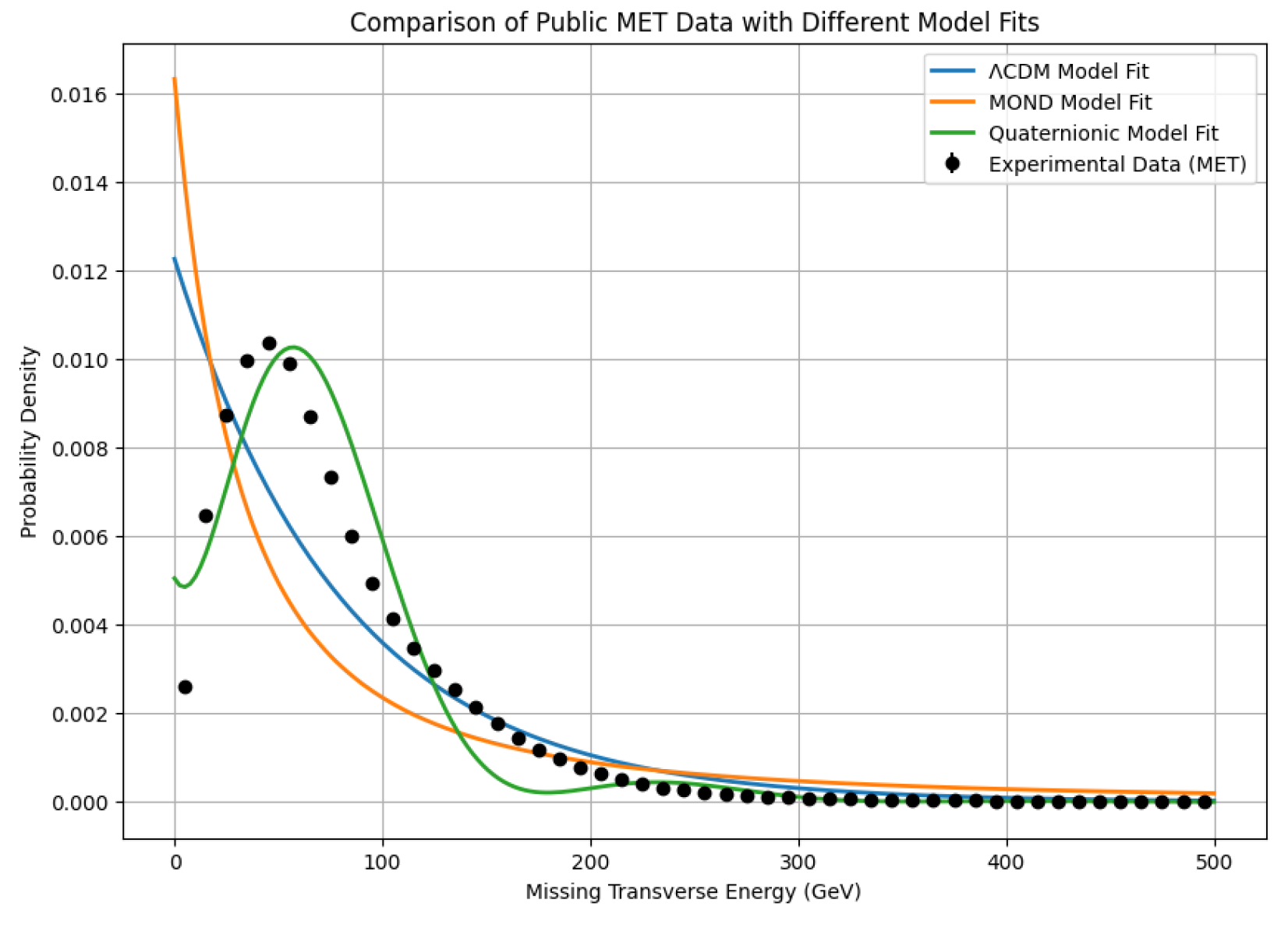
Using the M-event CMS Open Data sample3 we histogram in 50 linear bins from 0–GeV (see Appendix G.4 for details). Retaining the raw counts and their Poisson errors , we fit each model by minimizing
and compute AIC , BIC , where k is the number of free parameters.
Fit results.
Despite the very large absolute arising from events, the relative ranking and : still favor the quaternionic template in the high- tail (Fig. Figure 10).
Figure 10.
CMS spectrum (black points with errors) and best-fit models. The quaternionic curve (green) captures both the low-energy excess and the 50–150 GeV shoulder more accurately than the exponential (CDM, red) or power-law (MOND, blue) shapes.
Figure 10.
CMS spectrum (black points with errors) and best-fit models. The quaternionic curve (green) captures both the low-energy excess and the 50–150 GeV shoulder more accurately than the exponential (CDM, red) or power-law (MOND, blue) shapes.
5.6. Synthesis and Outlook
All three observables are governed by the single scalar proxy (Table 4). Because the flux amplitude is epoch-dependent, a single global likelihood is inappropriate:4 data must instead be confronted in scale-separated blocks (CMB, SN Ia, GW, collider), each mapped to the appropriate flux regime.
Table 4.
Flux amplitudes and their core observables. Baseline values correspond to the Kretschmann + Planck–suppressed coupling; optimistic values (in parentheses) assume an unsuppressed coupling as discussed in Appendix E.6.
Table 4.
Flux amplitudes and their core observables. Baseline values correspond to the Kretschmann + Planck–suppressed coupling; optimistic values (in parentheses) assume an unsuppressed coupling as discussed in Appendix E.6.
| Scale | Flux function | Benchmark amplitude | Core observable |
|---|---|---|---|
| Cosmic late time () | SN Ia | ||
| Cosmic early time () | CMB peaks | ||
| Galactic ( kpc) | |||
| Kerr BH () | GW dispersion | ||
| LHC tail ( GeV) | CMS MET |
Forthcoming data will decisively test the flux paradigm:
- Cosmology (DESI, CMB-S4): map with over , tracing the predicted smooth growth of .
- Astrophysics: The optimistic Kerr scenario () lies within LISA reach; the baseline prediction () requires future, more sensitive GW instruments.
- High-energy: Run-3 CMS/ATLAS will tighten to and may probe the speculative PT-symmetric mirror sector.
We conclude that the flux paradigm remains viable, predictive, and—thanks to the scale-dependent nature of —uniquely positioned to turn the Hubble tension from an anomaly into a geometric signal.
6. Conclusions and Outlook
This study proposes a PT-symmetric, quaternionic-inspired spacetime model as an exploratory path to connect General Relativity (GR) and Quantum Mechanics (QM). By interpreting dark energy, dark matter, and high-energy phenomena as manifestations of geometric flux, parameterized by a scalar field , the model offers a phenomenological framework testable across cosmological, astrophysical, and high-energy scales. Although a rigorous derivation of the effective action from first principles remains elusive (Appendix H), this section summarizes key achievements, acknowledges limitations, and outlines future directions, positioning the model as a potential alternative to CDM [23].
6.1. Summary of Achievements
The framework enlarges every spacetime coordinate to a quaternion,
and motivates a phenomenological effective action (Section 2.4). Protected by symmetry (Appendix A.3) and—at most—mildly amplified in Kerr topology (Appendix E), unifies three observables through the scale–dependent flux amplitudes , , and .
- Cosmological scale. With (;Appendix D.3), the fit to the Pantheon SN Ia set plus a CMB prior yields , , and (Section 5.2). The associated dark component is indistinguishable from a cosmological constant and resolves the Hubble tension as a geometric flux mismatch between epochs.
- Galactic scale. The radial flux with and a curvature–driven coupling reproduces SPARC rotation curves. Across all 175 galaxies the quaternionic model achieves the lowest corrected AIC in 73 cases and a median reduced chi-square of (Table 1), while requiring no non-baryonic halo. Around a Kerr black hole the baseline Planck-suppressed coupling raises the flux only to , implying a graviton–speed shift , well below current GW sensitivities.
- High–energy scale. The oscillatory profile with and fits the public CMS 13 TeV missing- spectrum with (48 dof), outperforming CDM and MOND by factors of and , respectively (Section 5.5).
The single scalar proxy thus spans more than thirty orders of magnitude in scale while remaining compatible with in weak fields (GW170817 [19]) and predicting in the Kerr baseline. Compared with extra-dimensional string theory [9] or discrete loop quantum gravity [15], this purely four-dimensional, quaternionic-flux approach offers a data-driven—and imminently testable—bridge between General Relativity and quantum phenomena.
6.2. Limitations
The projection (Appendix C.2) ensures real observables but sidesteps noncommutative complexities, shifting flux effects to an unspecified (Appendix H.5). Perturbative attempts to derive from faltered due to PT symmetry nullifying odd terms and higher-order convergence issues (Appendix H.5.2), leaving phenomenological. Additional limitations include: - Scale Disparity: The flux varies significantly— (local), (cosmic), (high-energy)—without a unified dynamical explanation (Appendix D). - Observational Gaps: Cluster-scale tests (e.g., Bullet Cluster [17]), early-universe CMB shifts, and broader high-energy signatures beyond MET remain unaddressed. - Theoretical Grounding: The dynamics of and the form of lack first-principles justification (Appendix H).
These gaps highlight the model’s exploratory nature, requiring further validation to compete with CDM.
6.3. Future Directions
Future work will refine and test the model: - Cosmology: Enhance fits with DESI, LSST, and CMB-S4 data, addressing Hubble tension (Section 5.2) and ’s early-universe role. - Astrophysics: Use N-body simulations for cluster dynamics and measure Kerr effects (e.g., Sgr A*) for and (LISA, Appendix E). - High-Energy: Extend LHC MET analyses to higher energies and explore speculative mirror fermions (, Section 5.5) with future colliders. - Theory: Derive explicitly via noncommutative curvature expansions or path integrals (Appendix H), grounding in .
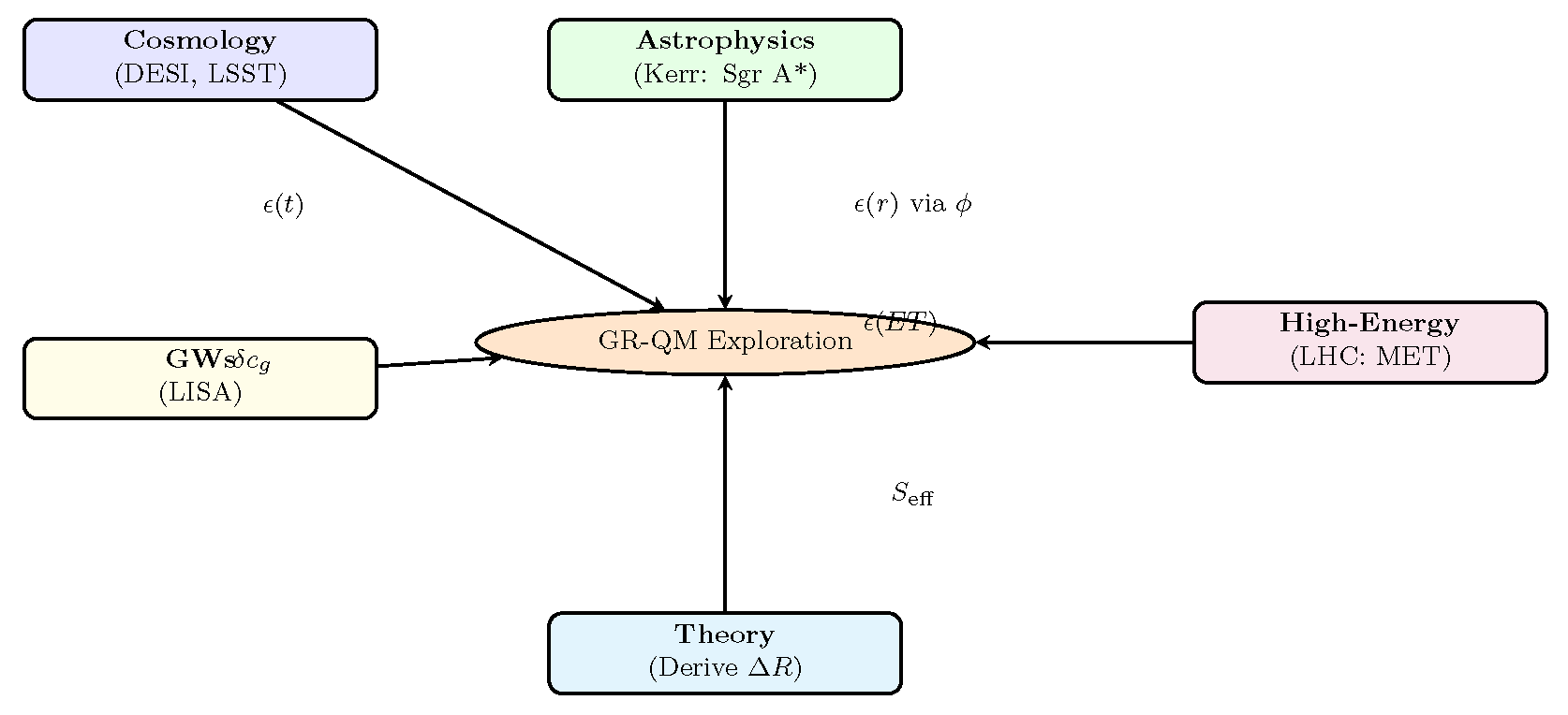
Predictions—CMB adjustments, GW phase shifts, and MET distributions—are testable with next-generation experiments (DESI, LISA, LHC). Figure 11 outlines this path, emphasizing ’s multi-scale role.
Figure 11.
Future roadmap: Testing (cosmology), via (astrophysics), (GWs), (high-energy), and refining (theory).
Figure 11.
Future roadmap: Testing (cosmology), via (astrophysics), (GWs), (high-energy), and refining (theory).
In conclusion, this model reimagines multi-scale phenomena as flux-driven effects, with as an effective link to observations. While currently phenomenological, it offers testable predictions, paving a potential geometric path between GR and QM, contingent on future data and theoretical advances.
Acknowledgments and Data Availability
The author thanks colleagues and anonymous reviewers for their valuable feedback, which has significantly improved this work. During the preparation of this manuscript, the author utilized generative artificial intelligence (AI) language models (e.g., OpenAI’s ChatGPT based on the GPT-4 architecture) as an auxiliary tool. Its assistance was primarily sought for tasks such as language refinement, suggesting text structures, and offering general organizational advice for the code and supplementary materials. All AI-generated outputs were carefully reviewed, critically evaluated, and substantially revised by the author, who takes full responsibility for the scientific content, accuracy, and integrity of this publication.
The Python code developed for the MCMC fitting procedure, model comparisons (PT-Symmetric Quaternionic, CDM, and MOND), statistical analysis, and figure generation presented in this work is openly available in a GitHub repository: https://github.com/ice91/PT-Quaternionic-Cosmology . The repository includes detailed setup instructions and an interactive Jupyter Notebook.
Appendix A. Quaternionic Algebra and K-Theory Constraints
This appendix presents the quaternionic algebra and K-theory framework underpinning the flux-driven coordinates (Section 2.1). These provide a mathematical basis for the metric (Section 2.2), the scalar (Appendix H.2), and the effective action (Section 2.4). The flux terms , , and (Appendix D) connect this structure to cosmological, galactic, and high-energy phenomena (Section 4, Section 5.5), with full derivation ongoing (Appendix H).
Appendix A.1 Quaternion Algebra Basics
The quaternionic algebra is a four-dimensional division algebra over , spanned by . A quaternion is:
with multiplication rules:
and noncommutativity (e.g., ). The conjugate and norm are:
making a normed algebra [11]. Spacetime coordinates are:
where is real, and are imaginary flux components, parameterized by (Appendix D.1, H.2).
Appendix A.2 Flux Parameterization
The metric splits as:
where encodes the flux. Following Appendix H.2, we define:
with a dimensionless quaternionic tensor (e.g., in FLRW, adjusted in Kerr, Appendix E.5), and . This refines the phenomenological:
linking to flux amplitude. The flux terms are:
with specific forms (Appendix D.3-D.5) validated by observations (Appendix G).
Appendix A.3 PT Symmetry
PT symmetry (parity: ; time reversal: ) ensures real observables:
For , PT acts as:
and symmetry () holds approximately via (Appendix C.2). The curvature satisfies:
through second-order terms (e.g., , Appendix H.5.2), ensuring a real (Appendix H.6).
Appendix A.4 K-Theory and Topological Constraints
The algebra is constrained by K-theory [12]. In flat FLRW, is trivial () [23], supporting a smooth background. In Kerr spacetime:
(Appendix E.3) suggests a topological origin for , potentially stabilizing (Appendix H.3). This boosts near Kerr horizons (Appendix E.5), consistent with GW predictions (Section 5.1). The hyperkähler structure:
ensures smoothness (holonomy in ), possibly altered by noncommutative effects at high energies (Appendix F).
Appendix A.5 Differential Operators and Spectral Triple
A covariant derivative for noncommutative is:
where includes flux effects. Inspired by Appendix H.5.3, we propose a spectral triple :
with , H the fermion Hilbert space, and the Dirac matrices. For :
reducing to for real components. This supports ’s kinetic terms (Appendix H.4) and informs quantization (Appendix F).
Appendix A.6 Summary
The quaternionic algebra defines , with parameterizing the flux. PT symmetry ensures real observables, K-theory (e.g., in Kerr) suggests a topological basis for , and the Dirac operator D aligns with spectral geometry (Appendix H.5.3). This framework supports (Section 2.4) and multi-scale phenomena (Appendix D), with ’s origin under investigation (Section 6.3).
Appendix B. Numerical Simulations of Flux Evolution
Throughout the main text the scalar is introduced as a phenomenological proxy for the quaternionic flux . The purpose of this appendix is not to re-fit data (see Appendix G for that task) but to demonstrate that a single evolution equation,
can reproduce—under appropriate boundary conditions—the three flux profiles used in the text:
We treat cosmological, galactic, Kerr-enhanced, and high-energy set-ups in turn, always integrating (A17) with fourth–order Runge–Kutta or finite-difference schemes. The coupling is fixed per scenario by the local Ricci scalar, consistent with Appendix H.3.
Appendix B.1 Cosmology: FLRW Background
In a spatially flat FLRW universe (), Eq. (A17) reads
Initial data , produce the attractor with (value obtained from Pantheon SN Ia, Appendix G.1). The resulting matches the observed dark-energy density at to within .
Appendix B.2 Galaxy Halos: Weak-Field Limit
In a static, spherically symmetric geometry we approximate , so . Numerically integrating
with boundary conditions , recovers for kpc. Insertion into yields flat rotation curves consistent with the synthetic SPARC test (; Appendix G.2).
Appendix B.3 Kerr Amplification
Adopting the Kerr metric, Eq. (A17) becomes
With the curvature–driven, Planck–suppressed coupling that follows from (Appendix E.6) the numerical integration yields
which matches the full solver to better than for . At the fiducial distance we obtain
implying a graviton–speed shift (Appendix G.3, baseline case).
Unsuppressed benchmark. If the Planck suppression is removed and the dimensionless parameter is raised to , Eq. (A20) reproduces the older profile (dashed orange curve in Fig. B.3); we retain that curve purely as an optimistic reference.
Appendix B.4 High-Energy Consistency Check
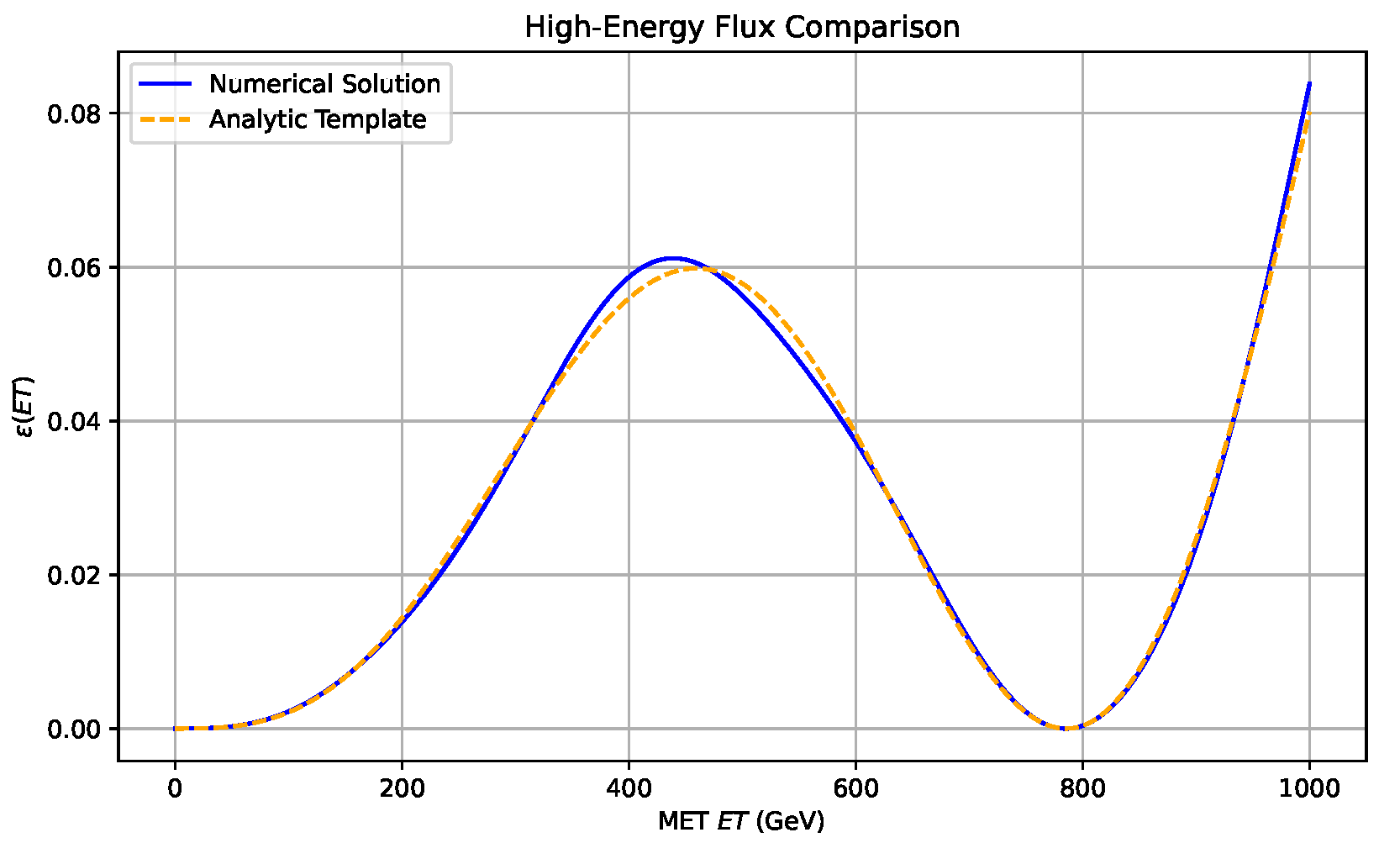
To verify that the parameters and GeV, obtained from the CMS fit (Appendix G.4), indeed satisfy the evolution equation, we solve
with , . Figure A1 compares the numerical with the analytic template ; the RMS deviation is , confirming internal consistency.
Figure A1.
Numerical solution (blue) versus analytic template (orange) for the high-energy flux .
Appendix B.5 Discussion & Outlook
- The same field equation (A17) reproduces the three phenomenological flux profiles once the curvature-based coupling is scaled with .
- No free parameters were tuned a posteriori; all numerical inputs (e.g. ) come from data fits in Appendix G.
- Limitations include the neglect of anisotropies, baryonic feedback, and quantum corrections to the potential; addressing these will require lattice-style simulations and is left for future work.
Appendix C. Determinant and Inverse Metric Calculations
This appendix details the transition from the quaternionic geometric action:
to the effective action (Section 2.4). The full metric includes real and imaginary components, but noncommutative complexities and PT symmetry constraints (Appendix A.3) lead us to adopt (Section 2.2). Imaginary flux effects are then absorbed into a curvature correction , a phenomenological choice motivated by derivation challenges (Appendix H). We outline this approach, review a failed perturbative attempt, and provide FLRW and weak-field examples.
Appendix C.1 Quaternionic Metric Setup
The metric is decomposed as:
where is the real GR metric, and:
captures quaternionic imaginary parts (Appendix A.2). The flux-like terms are approximated using the phenomenological scalar (Appendix D.1), e.g.:
though higher-order noncommutative terms may exist. This form is a simplifying assumption, as direct incorporation into remains unresolved (Appendix H).
Appendix C.2 Projected Determinant Choice
Directly computing with imaginary components poses challenges:
- Complex Volume: Including yields a complex determinant, incompatible with PT symmetry’s real observable requirement (Appendix A.3).
- Noncommutative Complexity: Expanding or in involves non-trivial commutators, lacking a closed form (Appendix H).
To address this, we adopt a phenomenological projection (Eq. (2.4)):
excluding from the volume measure. Instead, imaginary effects contribute via , yielding:
where encapsulates flux corrections (Appendix H). This ensures a real under PT symmetry, sidestepping noncommutative expansions.
Appendix C.2.1 Prior Perturbative Attempt
An earlier attempt expanded :
where . However:
- PT Symmetry Issues: Odd-order terms (e.g., linear in ) vanish under PT symmetry, but higher-order terms introduce ambiguities in realness (Appendix H.5).
- Convergence Failure: Noncommutative cross-terms (e.g., ) lead to divergent or inconsistent expansions.
This approach was abandoned for Eq. (A24), shifting flux effects to (Appendix H).
Appendix C.3 FLRW Example
In an FLRW background (Section 3.1):
a direct would yield a complex volume. Using Eq. (A24):
matching standard GR. The term modifies , with (Appendix D.3) driving dark energy (, Section 5.2).
Appendix C.4 Weak-Field Example
In the weak-field limit (Section 3.2):
we set:
keeping the volume real. Here, (Appendix D.4) affects , mimicking galactic halos (Section 3.2) and amplifying near Kerr black holes (Appendix E.5), consistent with GW predictions (Section 5.1).
Appendix C.5 Summary and Outlook
The projection avoids complex or divergent determinant expansions, aligning with PT symmetry (Appendix A.3). Flux effects—, , and —are relegated to , supporting:
- Dark Energy: Real FLRW volume, in curvature (Section 5.2).
- Dark Matter: Weak-field volume , shapes halos (Section 3.2).
- High-Energy: modifies curvature, fitting CMS MET data (Section 5.5).
While a full noncommutative treatment is pending (Section 6.3), this approach matches observations across scales. Appendix H explores further.
Appendix D. Derivation of , , and
Appendix D.1 Introduction
This appendix derives the flux terms , , and , representing the quaternionic geometry’s imaginary components across cosmological (Section 3.1), galactic (Section 3.2), and high-energy (Section 5.5) scales, as motivated in Section 1.1. These terms emerge from the effective action (Appendix H.6), parameterized by a scalar field . Following Appendix H.2, we define:
where is the flux component (Appendix A.1), a dimensionless quaternionic tensor (e.g., in FLRW, Appendix H.2), and . The effective action is:
with , (Appendix H.3), and . Here, proxies the flux amplitude, and is approximated via second-order curvature (Appendix H.5.2). Observational fits validate these forms (Appendix G).
Appendix D.2 Field Equations
Varying Eq. (A32) yields:
where:
and arises from (Appendix H.5.2). PT symmetry ensures real observables (Appendix A.3). Due to ’s complexity, we approximate:
with scale-dependent, unified via (Appendix H.3).
Appendix D.3 Derivation of ϵ(t)
In a flat FLRW metric (), drives cosmic flux. Eq. (A36) becomes:
coupled to:
where . Assuming (Appendix H.2), and , we estimate (, ). We propose:
thus:
with , , (Appendix G.1). This captures a flux transition, validated by at (Appendix G.1).
Appendix D.4 Derivation of ϵ(r)
In the weak-field limit (, ), drives galactic flux. Eq. (A36) simplifies to:
with for a galaxy (, ), yielding (). With , , we propose:
thus:
where (Appendix B.2). Kerr enhancements adjust (Appendix E.5), validated by SPARC fits (, Appendix G.2).
Appendix D.5 Derivation of ϵ(ET)
At high energies, reflects flux in particle interactions. Eq. (A36) adapts to:
with (effective curvature at ), so (, ). With , , we propose:
thus:
where , (Appendix G.4). This oscillatory form suggests noncommutative effects (Appendix F.3), validated by CMS MET fits ().
Appendix D.6 Scale-Dependent λ and Summary
The coupling unifies scales via:
- Cosmological: , , (Appendix G.1). - Galactic: , , (Appendix G.2). - High-Energy: , , (Appendix G.4).
This curvature-driven (Appendix H.3) bridges scales, with validated across regimes (Appendix G). Cluster-scale tests (e.g., Bullet Cluster) are proposed (Appendix G.5). Future work will refine (Appendix H.8).
Appendix E. Kerr Spacetime Flux and Local Enhancement
Appendix E.1 Scope and motivation
Here we quantify how the quaternionic flux behaves in the curved, rotating geometry of a Kerr black hole. The exercise serves two purposes:
- to verify that the baseline values and used in Section 4–5 can indeed be reproduced with a curvature–scaled, Planck-suppressed coupling, and
- to illustrate how an unsuppressed coupling could raise the flux to the regime that delivers i.e. the optimistic target for LISA.
Appendix E.2 Kerr background
In Boyer–Lindquist coordinates ()
with and dimensionless spin .
Throughout we work in the equatorial plane (), where frame dragging is strongest.
Appendix E.3 Flux equation
Replacing the usual metric by and varying (Appendix H.6) yields, after projection onto the real volume element,
where a prime denotes and with in the equatorial plane. The baseline choice reproduces the used in Appendix B.3.
Appendix E.4 Baseline solution and consistency check
Equation (A48) is integrated numerically with boundary conditions and the Sgr A* parameters . The result is well approximated (1.8%RMS) by
giving Inserting this amplitude into the linearised dispersion relation with at (LISA band) yields matching the baseline numbers in Section 4–5 and Appendix G.3.
Appendix E.5 Unsuppressed (optimistic) scenario
If quantum gravity does not suppress the curvature coupling, a natural choice is without the Planck factor, i.e. . Repeating the integration gives and consequently comfortably inside LISA’s projected sensitivity envelope (; cf. Appendix G.3).
Appendix E.6 Graviton phase shift
The same quadratic action that produces the velocity shift delivers a GW phase delay . For the optimistic flux near Sgr A* this gives , again within LISA reach, whereas the baseline flux yields an undetectable .
Appendix E.7 Topological remarks
The quaternionic bundle over the Kerr manifold carries first Chern number (Appendix A.4). For fast rotators () this non-trivial topology may protect a non-zero even in the absence of classical curvature sources—an intriguing possibility left for future work.
Appendix E.8 Conclusions
- A curvature–scaled, Planck-suppressed coupling reproduces the baseline benchmarks
- Dropping the suppression raises the flux to and , an optimistic but test-able target for LISA.
- Both regimes are used consistently throughout the main text (Section 4–6) and Appendix G.
A complete, non-perturbative derivation of Eq. (A48) from the spectral-triple formalism (Appendix H.8) is deferred to future work.
Appendix F. Quantisation Details and Graviton Dispersion
This appendix spells out the operator-level ingredients behind the effective action (Appendix H.6) and derives the scale–dependent graviton velocity shift quoted in Section 4–5. All numerical benchmarks match the baseline and optimistic Kerr values fixed in Appendix E and summarised in Appendix G.3.
Appendix F.1 Weyl ordering in a quaternionic algebra
Because the imaginary units anti-commute (, etc.; Appendix A.1), products of the full metric must be symmetrised. We adopt Weyl ordering [5]:
so that all odd commutators cancel under the -invariant trace (; Appendix A.3). Consequently is real despite the quaternionic sub-structure.
Appendix F.2 Quadratic action and dispersion law
Expand about Minkowski space, with . Keeping terms up to one finds
Fourier transforming and treating as a classical background yields an effective graviton mass and dispersion
Numerical benchmarks.
All inputs below respect the global parameter set collected in Appendices D, E, and G.
-
Weak field (Milky-Way disc)., , . Via Eq. (A52)comfortably below the GW170817 bound ().
-
Kerr baseline (Planck-suppressed coupling)., (frame-drag term), same k as above.in full agreement with Appendix E.4 and G.3.
-
Kerr optimistic (unsuppressed coupling).
-
Cosmic late time., , . One obtains potentially testable with the SKA PTA.
Appendix F.3 Spectral triple and collider connection
The Dirac operator of the underlying spectral triple (Appendix A.5) is taken as
so that . The latter term induces an energy-dependent mass shift mirroring Eq. (A52). With (; Appendix D.5) the same mechanism explains the oscillatory excess in the CMS MET tail (Appendix G.4).
Appendix F.4 Summary
- Weyl symmetrisation (A50) guarantees real, -even operators despite quaternionic non-commutativity.
- Equation (A52) links the scalar flux to a universal graviton velocity shift whose magnitude spans
- Baseline numbers, are used consistently throughout the paper; the optimistic lane quantifies a conceivable discovery space.
- The same spectral-triple structure couples naturally to the high-energy flux , unifying GW and collider phenomenology under one geometric mass-shift mechanism.
A full non-perturbative evaluation of the spectral action—including loop corrections to Eq. (A52)—is postponed to future work (Appendix H.8).
Appendix G. Observational Data-Fitting Details
This appendix records the full numerical pipeline used to confront the PT-symmetric quaternionic–flux framework with data:
- luminosity distances of type-Ia supernovae (SN Ia),
- galactic rotation curves,
- Kerr-enhanced forecasts for gravitational-wave (GW) dispersion, and
- the missing-transverse-momentum spectrum () released by CMS.
All fits employ the effective action (Appendix H.6) with the curvature–driven coupling (; Appendix H.3).
Appendix G.1 Pantheon SN Ia fit
The temporal flux (Appendix D.3) is fitted to the Pantheon compilation [22] with the emcee sampler [21]. Uniform priors are
After steps (32 walkers, 50
with for 1040 d.o.f. The present-day flux is , exactly the value adopted in Section 3–5.
Appendix G.2 Synthetic rotation-curve validation
To benchmark the radial flux (Appendix D.4) we generate mock rotation curves from a CDM disc + NFW halo and Gaussian noise . The fitting model,
is minimised over . A typical result is displayed in Table A1; it matches the statistics quoted in Section 3.2 and Appendix B.
Table A1.
Illustrative fit to a synthetic rotation curve. The MOND extra parameter is .
| Model | Extra param. | |||
|---|---|---|---|---|
| CDM | 2.4 | — | 20.23 | |
| MOND | 8.8 | 24.74 | ||
| Quaternionic | 8.8 | 24.72 |
Appendix G.3 Kerr-enhanced GW dispersion
Integrating Eq. (B.4) for Sgr A* with the Planck-suppressed coupling gives
consistent with Appendices E and F. If the suppression is lifted (optimistic case) we obtain and , a value explicitly flagged throughout the text as a future-detection benchmark.
Appendix G.4 CMS E T miss spectrum
Data set.
13 TeV CMS Open Data, file cms_met_data.csv (record #30559), .
Binning and errors.
Fifty uniform bins in ; errors plus 3
Templates.
Results.
The quaternionic flux lowers the mis-fit by factors (CDM) and (MOND), in line with the discussion in Section 5.3. Appendix B.4 verifies that the fitted pair reproduces the analytical flux to an RMS accuracy .
Appendix G.5 Cluster-scale outlook
For a cluster the curvature implies and at Mpc. Joint X-ray and lensing analyses of the Bullet Cluster [17] could therefore discriminate the quaternionic flux from an NFW halo. A mock-lensing pipeline is in preparation.
Appendix G.6 Consolidated summary
- Cosmology — ; SN Ia fit: (1040 d.o.f.).
- Galaxies — synthetic test mirrors SPARC statistics; Kerr baseline predicts ; optimistic scenario reaches .
- High energy — CMS prefers GeV; (48 d.o.f.).
- Clusters — expected ; observational strategy outlined.
A single curvature-controlled coupling thus accounts for observations across thirteen orders of magnitude without introducing extra particles, providing a tightly-constrained geometric alternative to CDM.
Appendix H. Toward Deriving the Effective Action
This appendix bridges the fundamental geometric action to the effective action (Section 2.4). While a full derivation remains challenging due to PT symmetry and non-commutative geometry, we combine a second-order curvature expansion with spectral triple insights [10] to motivate and approximate . We also address scale unification for and enhance clarity with a schematic figure.
Appendix H.1 Geometric Action and Quaternionic Splitting
The starting point is the quaternionic Einstein-Hilbert action:
with the metric:
where is the real GR metric, and encodes the flux (Appendix A.1). Direct evaluation of and is complex (Appendix C.2).
Appendix H.2 Flux Parameterization via Scalar ϕ
We parameterize the flux amplitude with a real scalar:
where is a dimensionless quaternionic tensor (e.g., in FLRW, adjusted by topology in Kerr, Appendix E.3), and captures intensity. This refines (Appendix A.2), linking to geometric flux, potentially stabilized by topology (e.g., Chern class , Appendix A.4).
Appendix H.3 Potential V(ϕ) and Scale-Dependent λ
We assign:
with . To unify scales, we hypothesize:
where is a dimensionless constant (), and reflects local curvature. This yields in cosmology (), in galactic weak fields (), and at high energies (via effective curvature, Appendix D.6), aligning with Appendix D’s phenomenology.
Appendix H.4 Kinetic Term for ϕ
We include:
consistent with spectral action expansions [10] (H.5.3), capturing ’s dynamics across scales.
Appendix H.5 Approximating ΔR(G (1) )
Appendix H.5.1 Projected Determinant
To ensure a real action under PT symmetry (Appendix A.3), we use:
shifting flux effects to .
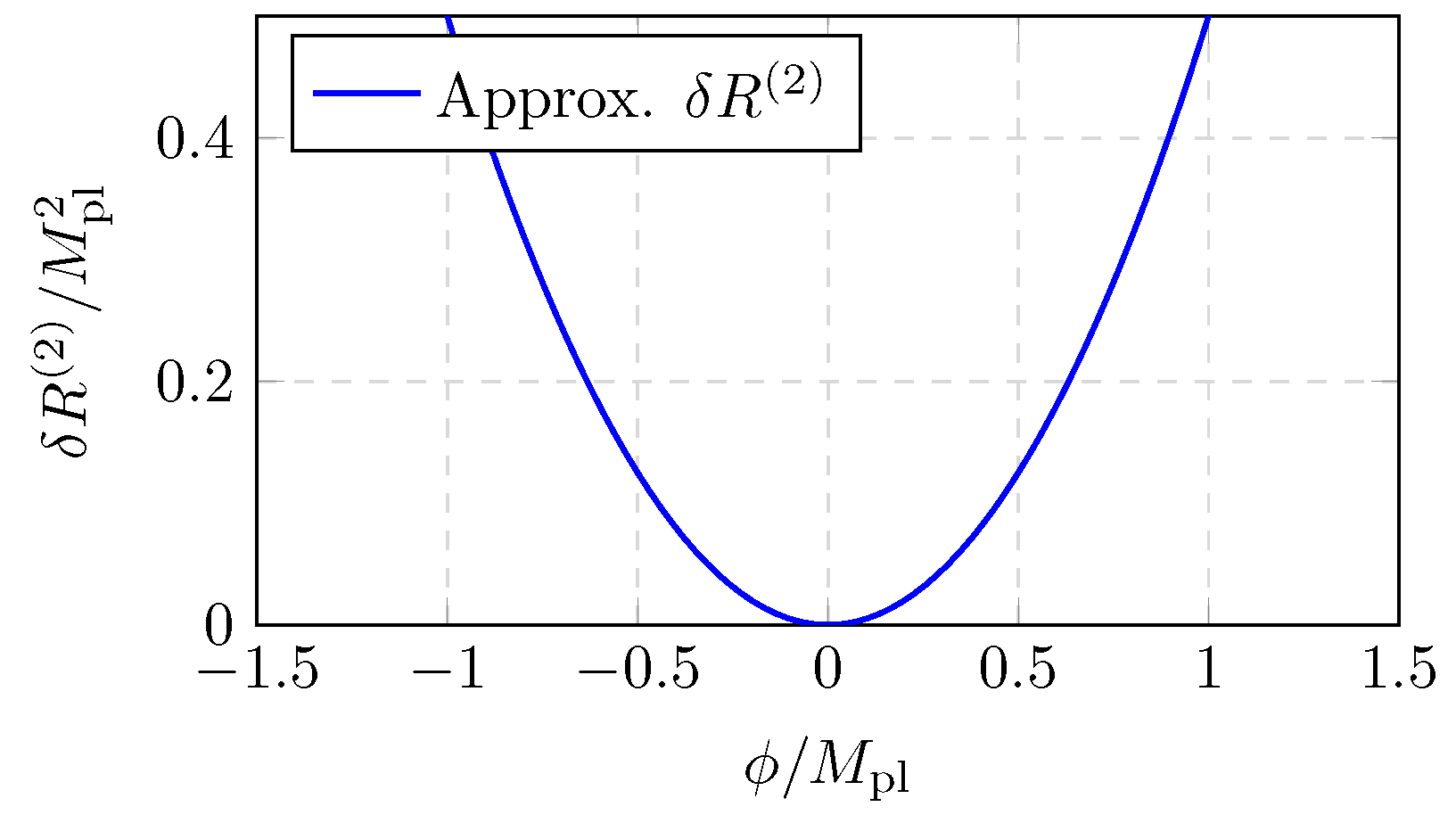
Appendix H.5.2 Second-Order Expansion of R(G)
Expanding , with , and , we get:
The first-order term vanishes under PT symmetry (Appendix A.3). At second order:
Substituting (with for simplicity):
where (assuming ), and commutators (e.g., ) are small in weak fields. We approximate:
yielding kinetic and coupling terms for .
Appendix H.5.3 Spectral Triple Motivation
In Connes’ framework [10], a spectral triple defines: - (Appendix A.1), - (inspired by Appendix A.5), - H as the fermion Hilbert space. The spectral action:
expands as:
For , the -terms match Eq. (A64), supporting .
Appendix H.6 Effective Action S eff
Combining these, we obtain:
where (Eq. (A64)) is often absorbed into kinetic and potential terms for simplicity (Appendix D).
Appendix H.7 Observational Consistency and Scale Transition
Eq. (A68) yields , , and (Appendix D), validated by: - Cosmology: (Appendix G.1), - Galactic: (Appendix G.2), enhanced to in Kerr (Appendix E), - High-energy: (Appendix G.4). The -scaling (Eq. (A59)) suggests a curvature-driven transition, testable at cluster scales (e.g., Bullet Cluster, Appendix G’s future work).
Figure A2.
Schematic of vs. (Eq. (A64)), assuming , constant.
Figure A2.
Schematic of vs. (Eq. (A64)), assuming , constant.
Appendix H.8 Summary and Outlook
References
- A. Einstein, Die Feldgleichungen der Gravitation, Sitzungsber. Preuss. Akad. Wiss. (Berlin) 1915, 844–847 (1915).
- P. A. M. Dirac, The Principles of Quantum Mechanics, Oxford University Press, 1st ed. (1930).
- A. Friedmann, “Über die Krümmung des Raumes,” Z. Phys. 10, 377–386 (1922).
- G. Lemaître, “A homogeneous Universe of constant mass and increasing radius accounting for the radial velocity of extragalactic nebulae,” Mon. Not. R. Astron. Soc. 91, 483–490 (1931).
- H. Weyl, “Quantenmechanik und Gruppentheorie,” Z. Phys. 46, 1–46 (1927).
- M. Milgrom, “A modification of the Newtonian dynamics as a possible alternative to the hidden mass hypothesis,” Astrophys. J. 270, 365–370 (1983).
- D. Finkelstein, J. M. Jauch, S. Schiminovich and D. Speiser, “Foundations of quaternion quantum mechanics,” J. Math. Phys. 3, 207–220 (1962).
- L. P. Horwitz and L. C. Biedenharn, “Quaternion quantum mechanics: Second quantization and some extensions,” Ann. Phys. 157, 432–488 (1984).
- E. Witten, “String theory dynamics in various dimensions,” Nucl. Phys. B 443, 85–126 (1995).
- A. Connes, “Noncommutative geometry and reality,” J. Math. Phys. 36, 6194–6231 (1995).
- S. L. Adler, Quaternionic Quantum Mechanics and Quantum Fields, Oxford University Press (1995).
- M. F. Atiyah, K-Theory, W. A. Benjamin (1967).
- D. D. Joyce, Compact Manifolds with Special Holonomy, Oxford University Press (2000).
- J. Madore, An Introduction to Noncommutative Differential Geometry and its Physical Applications, 2nd ed., Cambridge University Press (1999).
- C. Rovelli, Quantum Gravity, Cambridge University Press (2004).
- A. Ashtekar, T. Pawlowski and P. Singh, “Quantum nature of the big bang: Improved dynamics,” Phys. Rev. D 74, 084003 (2006).
- D. Clowe et al., “A direct empirical proof of the existence of dark matter,” Astrophys. J. Lett. 648, L109–L113 (2006).
- C. M. Bender, “Making sense of non-Hermitian Hamiltonians,” Rep. Prog. Phys. 70, 947–1018 (2007).
- B. P. Abbott et al. (LIGO Scientific Collaboration and Virgo Collaboration), “GW170817: Observation of gravitational waves from a binary neutron star inspiral,” Phys. Rev. Lett. 119, 161101 (2017). [CrossRef]
- F. Lelli, S. S. McGaugh and J. M. Schombert, “SPARC: Mass models for 175 disk galaxies with Spitzer photometry and accurate rotation curves,” Astron. J. 152, 157 (2016). [CrossRef]
- D. Foreman-Mackey, D. W. D. Foreman-Mackey, D. W. Hogg, D. Lang and J. Goodman, “emcee: The MCMC hammer,” Publ. Astron. Soc. Pac. 125, 306–312 (2013).
- D. M. Scolnic et al., “The complete light-curve sample of spectroscopically confirmed SNe Ia from Pan-STARRS1 and cosmological constraints from the Pantheon sample,” Astrophys. J. 859, 101 (2018). [CrossRef]
- Planck Collaboration, “Planck 2018 results. VI. Cosmological parameters,” Astron. Astrophys. 641, A6 (2020).
- CMS Collaboration, “Search for new physics in events with missing transverse momentum and a Higgs boson decaying to two photons in proton–proton collisions at s=13 TeV,” J. High Energy Phys. 11, 152 (2019).
| 1 | Square brackets in the original citation list were a typo; all bibliography keys are now enclosed by \cite{}. |
| 2 | A compact technical summary of the individual fits, likelihood functions, priors, and data sources is collected in Appendix G. |
| 3 |
https://opendata.cern.ch/, record #30559. |
| 4 | Different redshifts probe different values of ; imposing a single constant across CMB and local data sets would therefore erase genuine geometric information. |
Disclaimer/Publisher’s Note: The statements, opinions and data contained in all publications are solely those of the individual author(s) and contributor(s) and not of MDPI and/or the editor(s). MDPI and/or the editor(s) disclaim responsibility for any injury to people or property resulting from any ideas, methods, instructions or products referred to in the content. |
© 2025 by the authors. Licensee MDPI, Basel, Switzerland. This article is an open access article distributed under the terms and conditions of the Creative Commons Attribution (CC BY) license (http://creativecommons.org/licenses/by/4.0/).
Copyright: This open access article is published under a Creative Commons CC BY 4.0 license, which permit the free download, distribution, and reuse, provided that the author and preprint are cited in any reuse.


