
Submitted:
21 February 2025
Posted:
21 February 2025
You are already at the latest version
Abstract
We propose a novel heterodyne light source architecture employing two tandem acousto-optic modulators (AOM) operating under Bragg-diffraction conditions. A mirror and a half-wave plate are strategically positioned between the AOMs. By fine-tuning the angle of the mirror relative to the AOMs, only the +1st- or −1st-order light is generated, allowing the two light beams to coincide. The beat frequency is determined by the difference in modulation frequencies. In order to demonstrate the feasibility of this architecture, we use this light source in common-path heterodyne interferometry (CPHI) to measure the gold film thickness of a surface plasmon resonance (SPR) sensor. The experimental results are in good agreement with the outcomes of mathematical simulations.
Keywords:
heterodyne light source
; acoustic optic modulator
; Bragging diffraction
; SPR sensor
; phase measurement
; common-path heterodyne interferometry
1. Introduction
Heterodyne light sources commonly used in research include Zeeman lasers [1,2], Mach–Zehnder architectures [3,4], and electro-optic modulator (EOM) architecture [5]. Among these, the Zeeman laser functions as a self-contained heterodyne light source, offering a high beat frequency but at a high cost. The heterodyne light source based on the Mach–Zehnder architecture consists of two acousto-optic modulators (AOM); however, as it lacks a common-path architecture, it is susceptible to environmental disturbances. Additionally, the 0th-order light is not used, so the utilization rate of the laser is low. The heterodyne light source based on the EOM architecture requires full-wave voltage modulation, which causes a temperature rise in the electro-optic crystal, potentially leading to phase errors due to the high voltage.
Recently, Chiu et al. [6] proposed a heterodyne light source using two AOMs connected in series. While this setup is simple to implement, the diffraction efficiency remains suboptimal because the modulators are not operated under Bragg-diffraction conditions. In order to address these shortcomings, we propose an optimized configuration with two AOMs connected in series, both operating under Bragg-diffraction conditions. Through fine-tuning of the mirror and the two AOMs to ensure that the two orthogonally polarized light beams coincide, the heterodyne interference signal is substantially enhanced and the utilization rate of the laser approaches 90%.
2. Materials and Methods
In the acousto-optic modulator (AOM) shown in Figure 1a, the Bragg diffraction conditions are derived from the triangle in Figure 1b and are expressed as [7]:
then If and , then and:
where , , and are the wave vectors of the sound wave, diffracted beam, and incident beam, respectively, while and are the incident and diffracted angles, respectively. Here, is the sound velocity, is the frequency of the sound wave or the modulation frequency, is the wavelength of sound, and is the wavelength of the beam in the medium. If the frequency of the incident beam is , then the Doppler effect causes the frequency of the diffracted beam to be , where the beam is the +1st-order beam. Equation (2) represents the Bragg condition.
The basic optical setup of the heterodyne light source is shown in Figure 2 to further illustrate the principle of the coincidence of the two beams produced by the two AOMs connected in series. Here the modulation frequencies of AOM1 and AOM2 are and , respectively. Under Bragg diffraction conditions, if the optical frequency of the laser light is , then the optical frequency of the 0th-order beam from AOM1 is unchanged at , while the optical frequency of the +1st-order beam is The angle between these two beams is 2θ. The 0th-order beam from AOM1 is incident on the second AOM (AOM2). The optical frequency of the direct beam remains unchanged at which is denoted as beam A, while the optical frequency of the +1st-order beam is and is denoted as beam A′. The angle between these two beams is 2θ. In addition, the diffracted light with a frequency of is reflected into AOM2 after passing through mirror M. The direct light frequency remains , denoted as beam B, and its −1st-order beam has a frequency of , denoted as beam B′. By fine-tuning the angle of mirror M so that the angle of incidence is θ (that is, the angle between the 0th-order beams is 2θ), the two sets of beams can coincide. One set consists of beam A′ coincident with beam B, while the other set consists of beam A coincident with beam B′. The frequency difference between the two beams in both sets is.
As illustrated in Figure 3, the proposed heterodyne light source consists of a laser, two AOMs (AOM1, AOM2), a mirror (M), and a half-wave plate () positioned at an azimuth angle of 45°.
The acoustic waves of the two AOMs propagate in opposite directions. In this configuration, the laser operates at a frequency of , and the modulation frequencies of AOM1 and AOM2 are set to (80.00 MHz) and (80.01 MHz), respectively. Fine-tuning the AOMs enables them to operate under Bragg-diffraction conditions, the diffraction efficiency of the ±1st-order light reaches approximately 44%, while the 0th-order light achieves approximately 51% efficiency. When the 0th-order light from AOM1, which is p-polarized, passes through the half-wave plate, the outgoing light becomes s-polarized, making its polarization perpendicular to that of the +1st-order light. The +1st-order light from AOM1, after being reflected by mirror M, is directed into AOM2. Upon passing through AOM2, the frequencies of the 0th- and −1st-order light beams become and , respectively. In addition, after the 0th-order light of AOM1 passes through AOM2, the frequencies of the 0th- and +1st-order lights from AOM2 are and , respectively, as illustrated in Figure 3. By adjusting the angle of mirror M relative to the AOMs, the 0th-order p-polarized light () coincides with the +1st-order s-polarized light (), while the −1st-order p-polarized light () coincides with the 0th-order s-polarized light (). The Jones vectors of the electric field intensities and can be expressed as:
And
respectively, where and are the amplitudes of the electric field in the x and y directions, and and are the amplitudes of the electric field in the x and y directions, respectively. Once the two orthogonally polarized light beams coincide, two sets of heterodyne light sources are formed, with a frequency difference of 10 kHz.
3. Results
In order to demonstrate the feasibility of the proposed heterodyne light-source architecture, we use common-path heterodyne interferometry to measure the thickness of the gold film of a known surface plasmon resonance (SPR) sensor. The experimental architecture is illustrated in Figure 4.
We use an analyzer with a transmission axis set at a 45° angle to allow the orthogonal polarized light beams to interfere. The resulting interference signal was detected by a photodetector. The reference signal detected by is expressed as
and the test signal detected by can be expressed as:
where and are the average intensities, and are the visibilities, and is the phase-shift difference of the SPR sensor. The interference signals were recorded using an oscilloscope, as shown in Figure 5. According to the principle of the SPR sensor, the phase shift difference ϕ can be expressed as:
where and are the phase shifts of the p- and s-polarized light beams after passing through the SPR sensor.
As illustrated in Figure 6, the refractive indices of the prism (BK7), Au, and air are denoted by , and , respectively.
The total reflection coefficient of the p- or s-polarized light can be expressed as [8]:
where is the thickness of Au and:
where and are the refractive indices of Au and the prism, respectively; and are the angles of the light beams at the Au–prism interface; is the reflection coefficient at the boundary between mediums and j, where ; ; and For a laser wavelength of 632.8 nm, the refractive indices of the BK7 prism, Au, and air are 1.51509, , and 1.0003, respectively. Substituting these values into Equations (7)–(9) yields the total reflection coefficient and the phase shift difference . The resonance angle is near at for the boundary between Au and Bk7 and surface plasmon resonance conditions must be met
where and are the relative permittivity of Au and the Bk7 prism, respectively and is the wavenumber in vacuum.
By rotating the SPR sensor counterclockwise near the resonance angle (from to ), the phase-shift difference and the angle of incidence were recorded. The experimental data, denoted by red circles, are shown in Figure 7, alongside simulation results (solid line) generated using MATLAB. The optimal gold-film thickness obtained from the experiment was 35 nm, which is in good agreement with the actual gold-film thickness of the SPR sensor.
4. Discussion
These experiments confirm the feasibility of the proposed heterodyne light source as a reliable component for a common-path heterodyne interferometer. The phase resolution determined by stander deviation test was 0.04° as shown in Figure 8. From Table 1, the phase resolution of our structure is better than that of the Mach-Zehnder AOM structure and EOM architecture in our experiments. Although it is not better than Zeeman laser. But because of the low price, it still has its value. Under Bragg-diffraction conditions, the interference contrast could exceed 0.7 and the utilization rate of the light source was approximately 90%.
5. Conclusions
This heterodyne light-source architecture, featuring dual AOMs in tandem under Bragg-diffraction conditions, addresses the limitations of the Mach–Zehnder architecture regarding light-source utilization, as well as the low diffraction efficiency of previous dual-AOM architectures [6]. It offers ease of assembly and reduces the need for components such as beamsplitters, polarized beamsplitters, and an additional mirror, while only requiring the addition of a half-wave plate. This makes it a highly efficient and practical solution.
Author Contributions
Conceptualization, M.H. Chiu; methodology, M.H. Chiu; software, C.C. Chiu; formal analysis, M.H. Chiu; investigation, C.C. Chiu; resources, M.H. Chiu; data curation, C.C. Chiu; writing—original draft preparation, M.H. Chiu; writing—review and editing, M. H. Chiu; visualization, M.H. Chiu; supervision, M. H. Chiu; project administration, M.H. Chiu; funding acquisition, M.H. Chiu.
Funding
The current study was funded by the National Science and Technology Council (NSTC112-2221-E-150-035, Taiwan).
Data Availability Statement
Where no new data were created.
Acknowledgments
M.H. Chiu thanks the NSTC in Taiwan for supporting this work.
Disclosures
The authors declare no conflicts of interest.
References
- A. S. Badger; T. A. Rabson, Zeeman effect and ruby laser polarization, In Proceedings of the IEEE, 1964, 52(9), 1047-1048. [CrossRef]
- H. Takasaki; N. Umeda; M. Tsukiji, Stabilized transverse Zeeman laser as a new light source for optical measurement, Appl. Opt. 1980, 19, 435-441. [CrossRef]
- M. J. Ehrlich; L. C. Philips; J.W. Wanger, Voltage-controlled acousto-optic phase shifter, Rev. Sci. Instrum. 1988, 59, 2390-2392.
- M. G. Gazalet; M. Ravez; F. Haine; C. Bruneel; E. Bridoux, Acousto-optic low frequency shifter, Appl. Opt. 1994, 33, 1293-1298. [CrossRef]
- D.C. Su; M.H. Chiu; C.D. Chen, Simple two-frequency laser, Prec. Eng. 1996, 18, 161-163. [CrossRef]
- M.H. Chiu; C.C. Chiu, Tandem heterodyne light sources with dual acousto-optic modulators as an example of the optical rotation measurement of water as a function of temperature, Appl. Opt. 2024, 63, 6955-6959. [CrossRef]
- A. Yariv; P. Yeh, Optical Waves in Crystals: Propagation and Control of Laser Radiation, Wiley, John Wiley & son Inc.,USA, 2003, pp.329-336.
- H. Raether, Surface Plasmons on Smooth and Rough Surfaces and on Gratings, Springer Tracts in Modern Physics, Volume 111. ISBN 978-3-540-17363-2. Springer-Verlag, 1988.
Figure 1.
The +1st-order diffraction beam in acousto-optic modulator (AOM) under the Bragg diffraction condition.
Figure 1.
The +1st-order diffraction beam in acousto-optic modulator (AOM) under the Bragg diffraction condition.
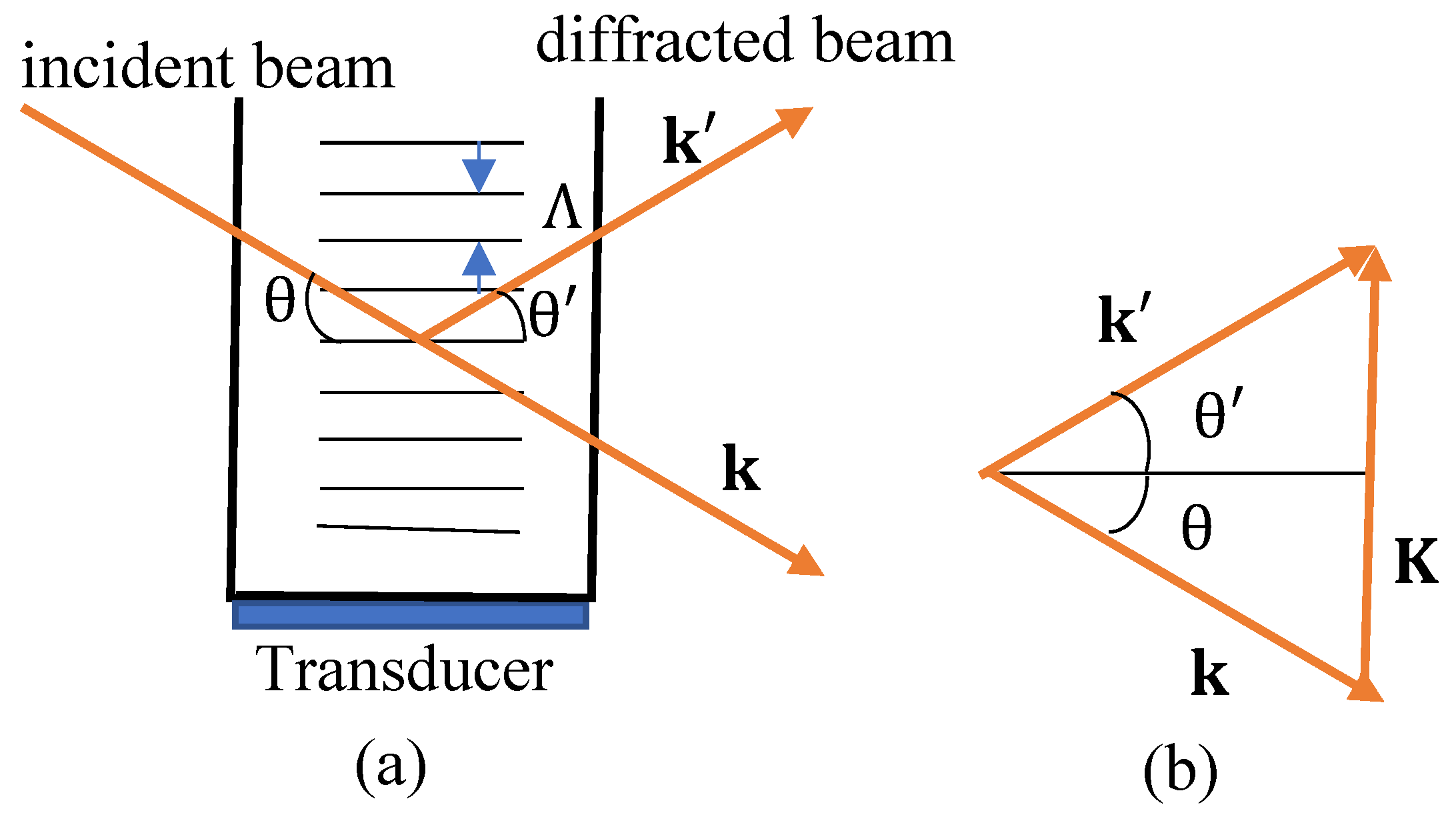
Figure 2.
The basic optical setup of a heterodyne light source.
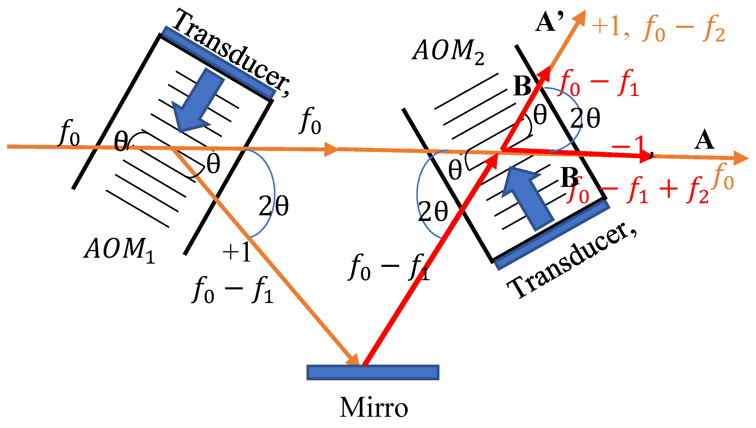
Figure 3.
Schematic of the heterodyne light source utilizing two tandem AOMs in Bragg-diffraction conditions. Components: helium-neon laser (λ = 632.8 nm); AOM1, AOM2: acousto-optic modulators; : half-wave plate; M: mirror.
Figure 3.
Schematic of the heterodyne light source utilizing two tandem AOMs in Bragg-diffraction conditions. Components: helium-neon laser (λ = 632.8 nm); AOM1, AOM2: acousto-optic modulators; : half-wave plate; M: mirror.
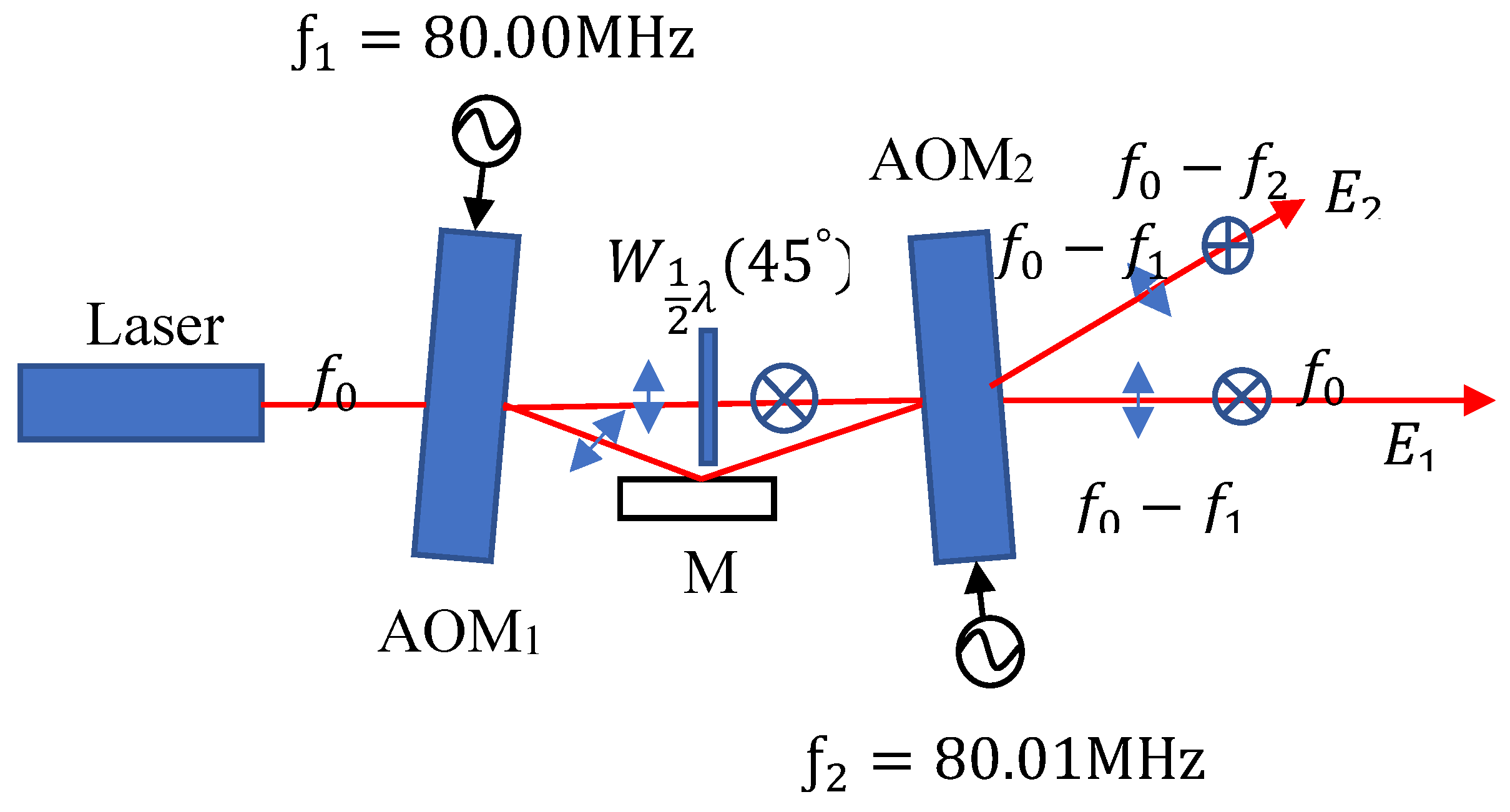
Figure 4.
Verification experiment: A common-path heterodyne interferometer based on the proposed heterodyne light-source architecture used for measuring the gold-film thickness of the SPR sensor. : analyzers; ,: photodetectors; SPR: SPR sensor; SR830: lock-in amplifier.
Figure 4.
Verification experiment: A common-path heterodyne interferometer based on the proposed heterodyne light-source architecture used for measuring the gold-film thickness of the SPR sensor. : analyzers; ,: photodetectors; SPR: SPR sensor; SR830: lock-in amplifier.
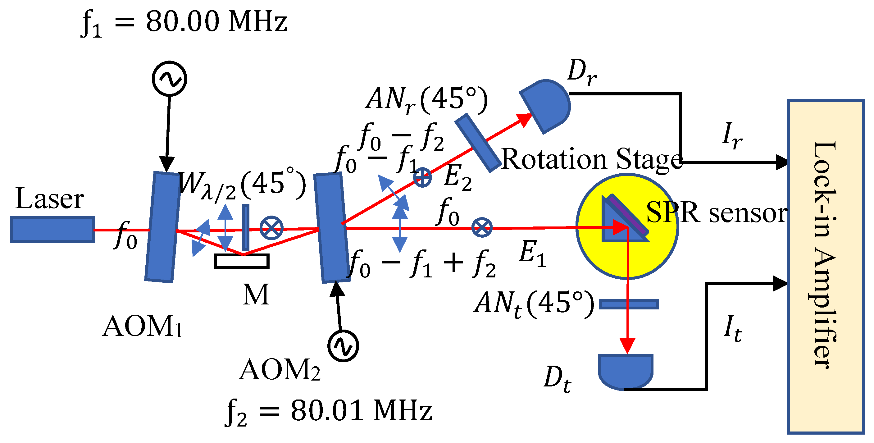
Figure 5.
Wave forms of the test and reference signals. The frequency of two signals is 10kHz.
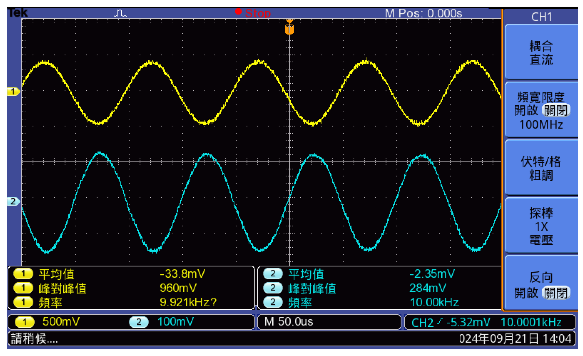
Figure 6.
Configuration of SPR sensor.
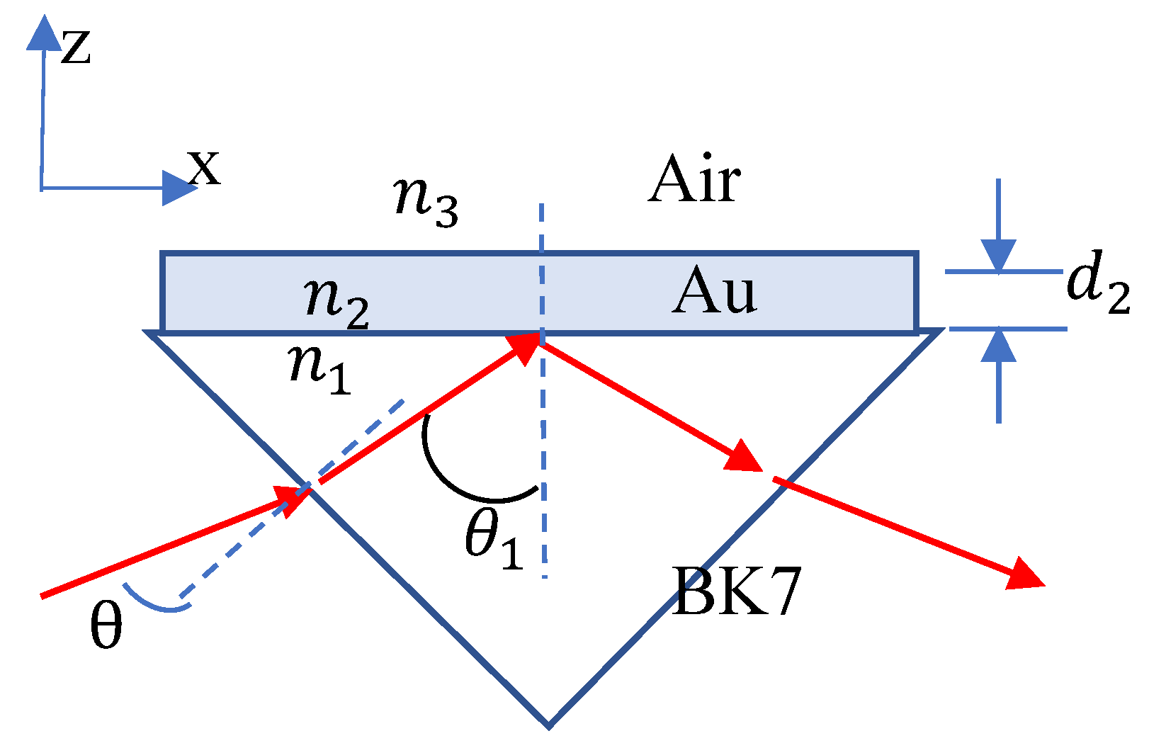
Figure 7.
Experimental results for the SPR’s gold-film thickness measurement using the common-path heterodyne interferometry (approximately 35 nm). Red circles: experimental values; blue line: simulation curve.
Figure 7.
Experimental results for the SPR’s gold-film thickness measurement using the common-path heterodyne interferometry (approximately 35 nm). Red circles: experimental values; blue line: simulation curve.
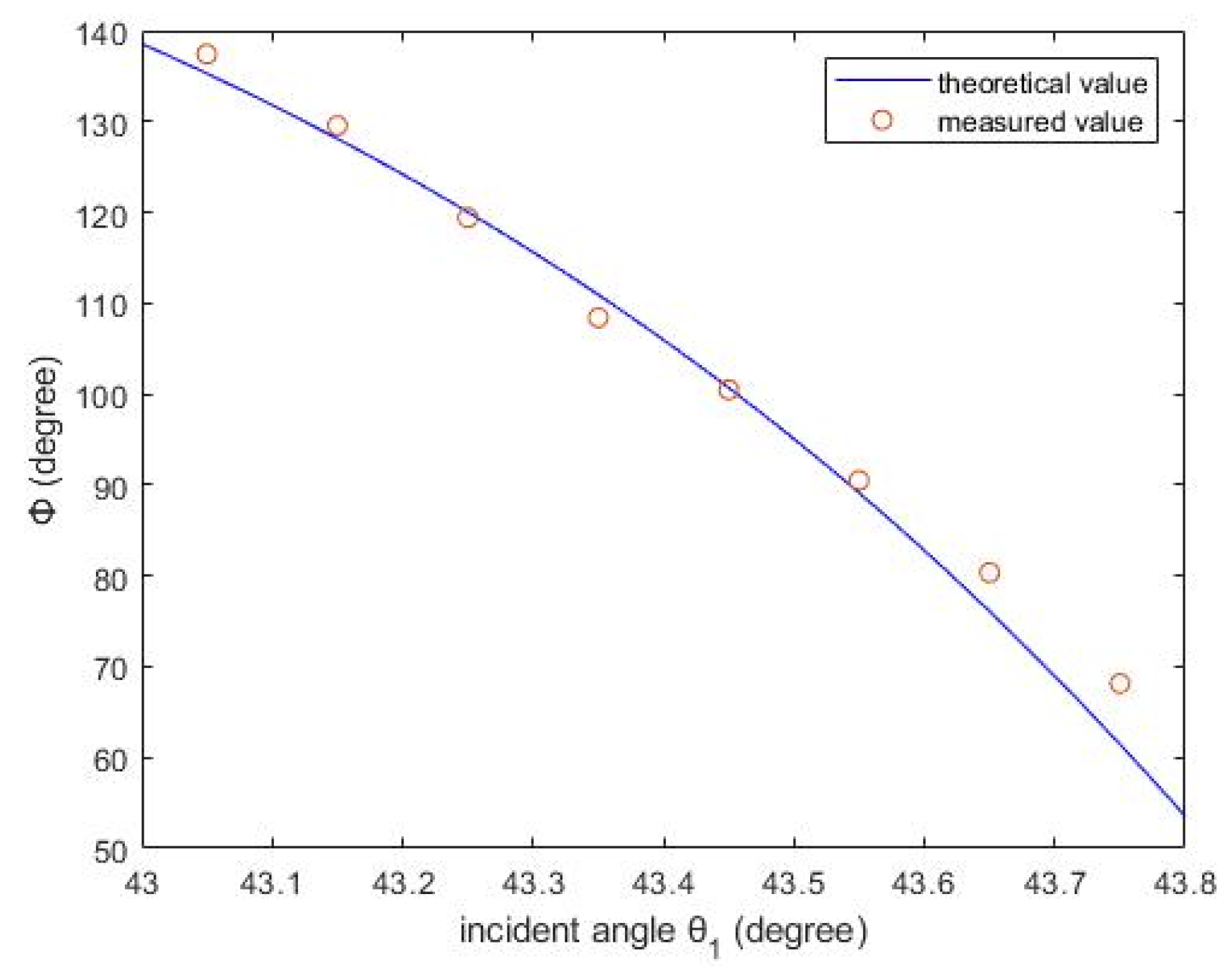
Figure 8.
The standard deviation of phase measurement.
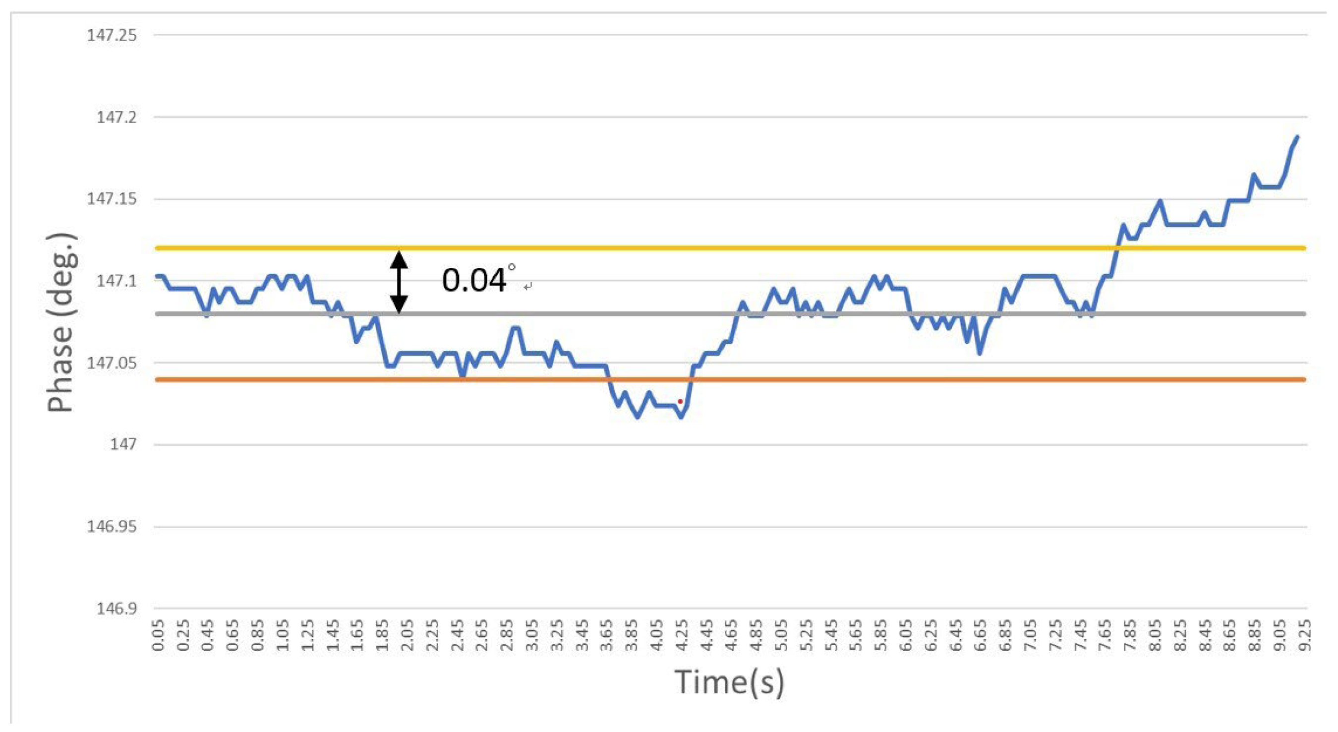

Table 1.
The standard deviation of phase measurement under a general heterodyne light source.
| Zeeman Laser | Mach-Zehnder AOM structure | EOM architecture | Our structure |
Disclaimer/Publisher’s Note: The statements, opinions and data contained in all publications are solely those of the individual author(s) and contributor(s) and not of MDPI and/or the editor(s). MDPI and/or the editor(s) disclaim responsibility for any injury to people or property resulting from any ideas, methods, instructions or products referred to in the content. |
© 2025 by the authors. Licensee MDPI, Basel, Switzerland. This article is an open access article distributed under the terms and conditions of the Creative Commons Attribution (CC BY) license (http://creativecommons.org/licenses/by/4.0/).
Copyright: This open access article is published under a Creative Commons CC BY 4.0 license, which permit the free download, distribution, and reuse, provided that the author and preprint are cited in any reuse.


