
Submitted:
20 May 2025
Posted:
22 May 2025
You are already at the latest version
Abstract
Heterodyne interferometry is widely used in science, industry, research, and development. It is mainly applied, but not limited to, displacement measurement, phase difference imaging, vibration measurement, surface quality control, metrology, and lithography. The phase shift between the reference and test beam signals provides information about the path length measurement. Using commercial heterodyne interferometer platforms for real-time applications leads to high costs and a lack of flexibility. To advance in the production of modular and low-cost interferometer systems, we applied a lock-in amplifier (LIA) technique to process heterodyne interferometer signals implemented with a field-programmable gate array (FPGA), providing a trade-off between high resolution and wide bandwidth. The developed method reaches sub-nanometric resolution when tested on simulations and synthetic signals; however, a nanometric resolution is ensured in a real-world test. The actual interferometer has a fundamental optical resolution of L/2, without resorting to the interpolation method. The LIA-FPGA system provides L/45 higher resolution than could be obtained with the fringe counting method, meaning 14~nm with a helium-neon laser of 632.9913774~nm wavelength. In addition, the LIA-FPGA system produces a high-rate measurement at 5200 samples per second, enabling its use in real-time high-speed controllers essential for existing and forefront sophisticated applications. Modular characteristics allow low-cost integration of multiple axes in a single embedded system based on an FPGA.
Keywords:
FPGA
; heterodyne interferometer
; hardware signal processing
; nanometer measurement
1. Introduction
The heterodyne interferometer (HI) is the most popular displacement measurement interferometry method, it is extremely noticeable when combined with an advanced field-programmable gate array (FPGA) architecture. The HI is a powerful tool widely used in many research areas, such as metrology [1,2], microscopy [3,4,5], or advanced manufacturing [6], to name a few.
The HI technique is based on two separated beams with orthogonal polarization. The difference between the fixed reference beam and the dynamic one is the frequency defied as a carrier frequency (beat), typically 2.7 MHz for the commercial He-Ne heterodyne laser heads. The frequency shift caused by the movement follows the Doppler phenomena and principles. When the mirror goes farther the frequency decreases and when the mirror goes near the frequency increases. At higher frequencies in the interferometer, less time is needed to keep its resolution in the measure. The separated optical beams produce the electrical output for the reference and the measurement signals. The optical path length is equivalent to the integral of the index of refraction and the variation in the displacement of the moving mirror (measurement arm). The phase angle between the reference and measurement signals determines the changes in the position or displacement of the test beam.
On one hand, there are many research focused on vibration measurement [7,8,9,10]. Chang et al. presented an heterodyne interferometer method to obtain vibration amplitude within nanometer resolution [7]. Zhou et al. developed a digital technique to improve vibration measurement resolution compared to sine approximation method [9]. Amorosi et al. present an accelerometer design that uses interferometry to measure low-frequency signals [10]. On the other hand, distance measurement using HI is a common application [11].
The lock-in amplifier (LIA) is one of the most precise and reliable methods to measure the amplitude and phase of a single-frequency signal accurately. Galaviz-Aguilar et al. [12] review many state-of-the-art works where LIA based on a phase-sensitive detector (PSD) is applied. Chen et al. [11] present a high-resolution application of the LIA using an HI to measure triaxial, movement getting sub-nanometric resolution. Chang et al. [13] proposed an analog LIA method applied to displace measurement heterodyne laser interferometry, obtaining high-resolution sub-nanometer measurements. The main drawback of this proposal is the signal attenuation when the interpolation stages are increased. In addition, the hardware processing technology used is insufficient to reach high-performance applications.
This work presents a new signal processing technique and its real-time FPGA implementation to obtain nanometer resolution with a heterodyne interferometer system. The proposed technique includes the signal processing algorithm, the custom hardware development, and the digital processing architecture. The rest of the paper is organized as follows: the phase measurement method is explained, then the proposed method is evaluated in simulation, the next section shows the digital signal architecture details, next conducted experimental tests are shown under various conditions comparing the whole system with a first certificate standard of heterodyne interferometer of the same nature, and finally, some conclusions are drawn based on the obtained results.
2. Phase Measurement
The proposed method is based on the lock-in amplifier principle [12], where a reference quadrature signal is mixed with the input and then low-pass filtered. In this way real and imaginary parts are obtained, thus amplitude and phase can be calculated in the input signal. The heterodyne interferometer head delivers two signals: reference and measurement. The reference signal comes from the interferometer reference optical path and the measurement signal comes from the moving mirror optical path. Since the motion of the mirror produces a Doppler effect in the measurement signal an interference pattern is produced between the reference and measurement signals. The proposed method uses the reference signal to measure with high resolution the phase of the measurement signal, then the phase is processed to get the displacement of the moving mirror.
The quadrature signal required by the lock-in method is generated from the reference signal by obtaining its derivative. Figure 1 illustrates the proposed method that, inputs measurement (MEA) signal and reference (REF) signal, both signals are band-pass filtered (BPF) to reduce their harmonic components.
The laser head input signals have a limited bandwidth sensibility thus the BPF is adjusted to this bandwidth to reduce the noise in subsequent calculations. Then the lock-in is applied to the measurement and quadrature signals by: first mixing (multiplying), second downsampling, and finally low-pass filtering (LPF). Taking input signals defined as:
By differentiating (1) we obtain:
then defining the quadrature reference signals as:
where (6) applies an amplitude compensation constant to normalize the signal respect to the reference defined in (5).
The lock-in method described in [12] was modified by introducing a downsampling operation between the mixing and the filtering steps, this is done to improve the filter response in the desired frequency band, and it also simplifies the real-time implementation. Then, the filtered signals are used to calculate the phase between reference and measurement signals by applying the function. Since the calculated phase angle is related to the frequency difference in the heterodyne interference due to the Doppler effect, the displacement is proportional to the phase based on the laser wavelength. The phase angle obtained with the lock-in method must be unwrapped since the function is range constrained to [-,]. To perform this operation the angle slope is calculated, and then the angle shifts are constrained to less than , further to accumulate the result, obtaining a continuous phase angle. In the following we call the proposed method lock-in downsampled phase detector (LDPD).
3. Simulation Test
The proposed method was tested on simulation with two different scenarios, synthetic signals and real signals. The synthetic signals were used to demonstrate the method function and real signals were used to measure resolution and stability.
3.1. Synthetic Signal Scenario
Following the structure depicted in Figure 1, some simulations were implemented in GNU Octave®, setting a reference signal of 2.7 MHz sampling at 60 MSps, and using a 632.9913774 nm wavelength. For the measurement signal three test with ideal conditions were performed, having zero, positive, and negative frequencies shifts.
The zero-frequency shift uses the same frequency for both input signals with a relative phase angle of rad.
Figure 2a shows the synthetic reference and measurement signals having a rad phase displacement. In contrast, Figure 2b shows the phase calculation () from the lock-in components (Ax and Ay), where the calculated angle remains constant at -0.7787 rad.
For the negative frequency shift at measurement, the signal below the reference frequency by 200 kHz was generated, and then both signals were fed to the LDPD. Figure 3a shows the synthetic signals where the phase shift produced by the frequency difference is evident.
Figure 3b shows the phase calculation result, where the phase change is evident with a negative slope, and the lock-in components show the phase lag that indicates a negative phase displacement.
For the positive frequency shift at measurement, the signal exceeding the reference frequency by 500 kHz was generated and then processed with the LDPD. Figure 4a shows a noticeable frequency difference. Since phase calculation in Figure 4b exhibited a positive slope and the lock-in components present a leading of Ay over Ax, in contrast to the seen in Figure 3b.
Those simulation results indicate the proper phase calculation by the LDPD method in three frequency conditions. An additional test was performed to measure phase resolution, generating synthetic signals of the same frequency with zero-phase shift. In this way, the maximum resolution by the LDPD method is computed. Figure 5 shows the raw phase calculation, it is zero-centered with a standard deviation of rad or 0.110 nm. To increment the phase resolution a low-pass filter is applied, then the filtered phase is obtained getting a standard deviation of rad or 1.012 pm. The applied LPF is an 11th-order FIR-type to minimize the transport delay for real-time implementation.
The performed simulations show the LDPD method response in an ideal scenario (without noise). To demonstrate its robustness a test is conducted by adding white noise to reference and measurement signals. This simulation uses a sample of 500 s signals polluted with white noise at four signal-to-noise (SNR) levels: 60 dB, 50 dB, 40 dB, and 20 dB.
Results in Table 1 show that for 50 dB and 60 dB SNR the figures are slightly above those obtained in the ideal scenario. In contrast, the test for 40 dB and 20 dB performs poorly, giving an error 150 times and 1500 times larger respectively. These results show that to achieve good results the input signals should be above 50 dB of SNR.
3.2. Real Signals Scenario
Another performed simulation test for the LDPD method was to record real-world signals from a laser heterodyne head and quantify its response. Figure 6 shows a real-world signal of 120 s recorded at 60 MSps using a 10-bit flash ADC. The ADC resolution was selected based on the results in Table 1 where a 10-bit ADC has a 60 dB SNR.
Figure 6b presents details of the first 5 s, where reference and measurement signals are clearly defined. Both signals have a square-type waveform with a slight overshoot. In this case, the measurement frequency is fading producing a negative change in the relative phase, indicating that the mirror is moving farther.
Since simulations in the previous section have perfect sinusoidal waveforms, some real-world signals were tested to identify potential problems related to SNR constraint and harmonic content. Figure 7a shows real-world signal fragments where phase change is evident along with its squared waveform and some noise spikes.
The first step in the LDPD is to apply a filter to get the fundamental frequency in the interest range between 2.4 MHz and 3.0 MHz removing most of the harmonic distortion and high-frequency noise. Figure 7b shows the filtered signals where most of the noise and the harmonic distortion have been removed getting smooth sinusoidal waveforms. The phase measurement result is shown in Figure 7c where lock-in components and phase were plotted. The computed phase starts at rad, then it moves to rad decreasing near to 0 rad; having a smooth slope in the 10 us interval.
Simulations using synthetic and real signals show that the LDPD method can calculate the phase accurately. Under ideal conditions, a 1 pm resolution is achieved, and considering noise (60 dB SNR), a 15 pm resolution is obtained. However, those figures do not consider noises coming from the acquisition system or numeric representations; those issues are addressed in the experimental section.
4. Digital Processing Architecture
The LDPD method was specifically designed to be implemented on FPGA executing it in real-time. The parallel computing ability of FPGAs is essential to achieve real-time performance in phase extraction.
Figure 8 details the main processing blocks in implementing the LDPD method. There are three main blocks: the acquisition system, the digital processing system, and the user interface.
Acquisition System
Since the heterodyne laser system generates the electrical signals, the first developed block was the analog-to-digital interface to acquire the signals properly. This block contains the signal conditioning, the anti-alias filter, and the fast analog-to-digital converter (ADC). The signal conditioner is based on a differential amplifier of high impedance that adjusts the signal amplitude for the ADC. The anti-alias filter is an essential component that rejects all frequency components above the interest band, meaning above 3.3 MHz. Finally, the ADC digitalizes the analog signals synchronously to avoid any phase jitter.
A proprietary acquisition system was developed to ensure the SNR quality in every analog stage, considering the 60 dB limit calculated in the simulations.
Digital Processing
The main block developed was the digital architecture for the LDPD on FPGA, this block executes all operations in real-time to complete the phase extraction and displacement measurement. Figure 8 details the principal operational blocks, by taking the digitalized reference and measurement signals. The first step is to synchronize the inputs and perform the reference derivative by a differential filter defined as:
where is the k-th input sample, is the k-th derivative signal output, and is the filter gain. The value for is defined as:
where is the sampling frequency and is the nominal reference frequency, in this implementation the value corresponds to 1.7684.
The next step is applying a band-pass filter that rejects all harmonic components beyond the interest frequency band. This task is performed by a finite-impulse response (FIR) filter of 11th order. By using a Bartlet window, the FIR filter was implemented using a pipeline architecture divided into 4 stages as depicted in Figure 9. Having a standard FIR formulae:
where is the i-th shifted input, is the output, are the filter coefficients, and n the filter order.
First, a delay stage that shifts the input every clock cycle. Second, a multiply stage where window coefficients are applied to the shifted input. Third, an accumulation stage that sums up the products. Finally, a saturation stage that corrects the numerical format. The accumulation stage is structured using a balanced binary tree balancing the transport delay chains in the FPGA logic. Every stage in the structure is registered to increase the clock frequency slack at the expense of latency increase. The input filter in Figure 8 is applied independently to each signal in parallel.
The next step is implementing the lock-in module, where parallel multipliers are used for mixing. Then downsampling is applied to the mixed products at a ratio of 9 to 1 with a linear interpolation. The saturation module adjusts the numerical format to avoid calculation overflow and prevent biasing in rounding. Then the low-pass filter extracts the signal quadrature components, implementing two 11th-order Bartlet FIR filters using the structure depicted in Figure 9. Finally, the phase calculation is performed by two parallel vectoring CORDIC units that take interleaved samples to speed up the calculation, then the results are merged into a single output. Since the CORDIC function takes 18 clock cycles it is necessary to split the calculation into two units to achieve real-time performance. The previous downsampling step provides 9 cycles for each sample, allowing a coherent clock domain in the lock-in module.
Once the lock-in module calculates the phase shift between input signals, it is necessary to unwrap the phase to estimate the mirror displacement. The differentiating unit in the unwrap module calculates the angle slope, which is proportional to the Doppler frequency shift hence the mirror velocity. To minimize the effect of angle discontinuities, the phase unwrapping method locates the changes larger than and compensates them by adding or subtracting . The unwrapped signal is low-pass filtered to remove high-frequency noise and downsampled to minimize drifting effects. The last step is accumulating the downsampled velocity to get the displacement value and scale the result based on the laser wavelength. The displacement gain is given by:
where represents the laser wavelength.
Then the position (POS) and velocity (VEL) values are connected to the FPGA internal system bus where an embedded microprocessor sends them to a host computer via a USB interface.
All modules inside the FPGA were developed in VHDL from scratch, and all operations were performed using fixed-point representation. The numeral representation in each operation was selected based on its SNR performance, which always keeps above 60 dB. Most operations use a numeral format of (3.13), meaning 3 bits for integers and 13 bits for fractions, which gives a 78 dB of SNR.
User Interface
The last stage of Figure 8 depicts the user interface that allows the user to control the measurement system. In this approach, a console application was implemented using C programming language that can be invoked by platform-specific applications providing the graphical user interface (GUI). The GUI was developed in GNU Octave® version 9.2, to display graphically the real-time measurements done by the FPGA system. The C program uses the libusb-1.0 library to control the FPGA device communication, then the data are transferred to the GUI in a JSON format.
5. Experimental Results and Discussion
The experiments conducted to test the performance of the proposed system were implemented in two scenarios: by using synthetic signals from a function generator comparing it with the laser system without movement and by integrating the full optics equipment compared against a national reference position standard.
5.1. FPGA Implementation System
The proposed system was implemented using a custom-designed FPGA board and a custom data-acquisition system that receives the interferometer output signals for reference (REF) and measurement (MEA), sampled at 60 MSps with 10-bit resolution, shown in Figure 10a.
The FPGA system is based on an AMD Spartan-7 XC7S50FTGB196-1 device, the HDL implementation was done in VHDL using v2022.2.1 (64-bits) on a Linux-Ubuntu 24.04.2 LTS. The FPGA system runs at 120 MHz using its internal phase-locked-loop (PLL) fed by a 48 MHz external clock source.
Figure 10b displays the FPGA resource utilization by the entire system implementation including the interferometry application, the USB communication interface, the embedded microcontroller, and the auxiliary units for memory management and system boot. The system uses 77% of the DSP resources and only 35.6% of the available LUTs leaving enough room to include future functionalities.
5.2. Zero-Motion Scenario
In this scenario, the electronic boards and the FPGA signal processing architecture were tested in a controlled environment to fully characterize its accuracy and intrinsic noise. The function generator produces the reference and measurement signals that the FPGA system captures measuring the phase change. The generated signals were set as if there was no displacement, having zero-phase and zero-frequency variation. In this way, the output reading only is produced by the electrical noise and quantization noise in the computing system, giving the maximum resolution of the digital processing system.
Figure 11a shows the output phase and its corresponding displacement measurement for the synthetic signals and Figure 11b the real-world signals using the heterodyne interferometer Agilent 5519A laser head and its optics. Figure 11 shows that the real-world signal contains higher noise than the function generator, as expected; but in both cases having resolutions below 0.5 nm.
Statistical analysis was performed to estimate the actual performance of the measurement equipment. For the function generator test 50 capture cycles were taken with a duration of 250 s; in addition, 20 capture cycles of the real-world signal on an isolated environment using the heterodyne laser head were taken also.
Figure 12 shows the statistical results analysis, where mean values and standard deviation values for both tests are displayed. The mean values for both signal sources have similar behavior, where function generator signals have a median closer to zero than the real-world signal but both moves in the same range; however, the real-world signal has larger data dispersion. Although the standard deviation of the function generator is lower than the real-world signal, presumably the real-world signal has larger noise, it is in accordance. The function generator test gets a median for the mean value of 0.53 pm while the real-world signal has -7.37 pm; and for the standard deviation, the median figure for the function generator is 24.57 pm while for the real-world signal is 53.55 pm. Those values indicate that in the best conditions, the maximum resolution achievable is up to 54 pm using the current laser head and optics while 25 pm corresponds to the intrinsic noise due to the electronics, and signal processing algorithm.
5.3. Evaluation by Calibration Testing Using First Standard
This scenario was an experimental test that used a moving objective that continuously was tracked by two interferometry systems: a reference displacement system and the LIFIUAQ. Figure 13 shows the experimental setup, composed of two laser heterodyne head interferometers Agilent 5519A, a beam splitter, the moving mirror, the LIFIUAQ system and the host PC to execute the user interface. The motion mechanism is integrated by a stepper motor and a belt and pinion system; using an open-loop control system. In addition, no ambient compensation was applied to the measurements.
The reference system is a national standard of displacement located at Centro Nacional de Metrología (CENAM) which is the national metrology institute in Mexico, this system is properly calibrated as a primary standard. In this test, the developed system measurement is compared against the reference system to calculate the absolute error in the distance measurement while the mirror is moving forward and backward in the rail.
The test consists of moving the mirror along the 5.5 m length rail, making stops every 500 mm taking 12 steps to make a full forward path, and then the process is repeated in the backward direction. The mirror halts by 15 s in every 500 mm step to allow the system to settle. In this test, the motion system is not connected to interferometers on a closed loop, so the displacement system processes every sample by averaging the stop position within 13 s window after the motion has stopped. Figure 14 shows the position and speed of a single test covering the forward and backward paths.
Since, the motion mechanism is independent of the interferometry equipment, the measurement reports the difference between the intended stop position and the measurement by the interferometric system. In Figure 14 the initial position is close to zero (-27.074 nm) and the final position (10.58 m) has some deviation mainly due to the mechanical backlash of the cart on the rail. However, the measurements are compared against the CENAM reference, not to the mechanical system.
In the Table 2 shows the results of a single forward pass comparing measurements between the CENAM reference and the LIFIUAQ equipment.
The fifth column shows the error between the LIFIUAQ measurement and the CENAM reference, where the maximum deviation error is 754.84 nm at the 2500 mm step. The last column shows the effective resolution in the measurement for every stop in the test, where the average resolution value is 13.88 nm.
To demonstrate the high-speed capture capacity of the LIFIUAQ, Figure 15a shows the 12 transient behavior of the motion system at every stop. In Figure 15a(i) an inner box of the 500 mm transient is plotted alone to appreciate the accuracy of the capture, where the vibration is clearly appreciated in the range of micrometers.
The transient captures shown in Figure 15a are similar for all steps, having an underdamped shape. This transient period was discarded when computing the values in Table 2, taking just the last 13 seconds of the stop. As depicted in Figure 15b(i) the movable mirror continues its motion 12 seconds after the motor stops, due to mechanical backslash. To compute the effective resolution in the position measurement, the residual motion was discarded by applying a moving average filter to subtract the central tendency, obtaining only the variation in position. The effective resolution was computed with the root mean square of the moving average filter output.
In Figure 15b(ii) a superposition of all position measurements is plotted to visualize the variation range. The total range is within ±100 nm boundary, while the mean standard deviation of all signals is 13.88 nm. Those figures are on the same scale as those shown in Figure 12, obtained in the zero-motion test. Then, the reported error in Table 2 is caused by the residual motion in the computing window; however, the proposed system accurately tracks the behavior in every stop with high resolution.
The LIFIUAQ system provides in real-time position and speed measurement, as shown in Figure 14 with a maximum sampling rate of 5208 Sps making it suitable for closed-loop control applications. The developed method can track a moving object at resolution of 14 nm without any environmental factor compensation. Giving final resolution of which surpases the obtained by standard techniques of fringe counts [15]. Thereafter, some works achieve sub-nanometer resolution such [9] and [11] both requires large integration periods not able to provide real-time performance.
Deng and Peng [14] proposed an FPGA structure applied to interferometer signals with a lock-in approach, having a high-resolution measurement of 0.074 nm. However, they only test its system in a simulated environment with a signal generator, discarding most of the noise in a real environment. Some noise was added to test their system performance but this is far from real conditions since most interferometer signals have heavy harmonic content. In addition, they use a commercial FPGA Labview platform without providing actual details of the system’s performance. Our method and implementation deal with real signals it is implemented in a low-cost FPGA suitable for real-time applications. The work by Vera-Salas et al. [16] presents a measurement technique that achieves 69.5 nm resolution within the range of 20 m, but their method is very sensitive to noise and changes in the input signal phase producing cumulative error.
6. Conclusions
In this paper, we presented a real-time LIA-FPGA method optimized for measuring displacement at high speed with a heterodyne interferometer reaching nanometric resolution. The proposed digital processing method is suitable for obtaining sub-nanometer resolution, as shown in simulations with synthetic signals. Based on the LIA-FPGA system, we compared the commercial heterodyne interferometer with the certified interferometer maintained by CENAM as the first standard using the nominal values for wavelength and beat frequency from the manufacturer’s datasheet. Reaching a resolution of 13.88 nm at 5208 Sps, with high-speed motion tracking within large ranges up to 5500 mm displacements. Further environmental calibrations are required to increase the resolution of the measurement.
Author Contributions
Conceptualization, L. Morales-Velazquez and I. Serroukh; methodology, L. Morales-Velazquez; investigation, L. Morales-Velazquez, I. Serroukh, R. Pichardo-Vega. and E. Galan-Uribe; writing—original draft preparation, L. Morales-Velazquez and I. Serroukh; All authors have read and agreed to the published version of the manuscript.
Funding
This research was funded by U.S. Department of Energy, Office of Science, Office of Basic Energy Sciences (DE-AC02-76SF00515).
Acknowledgments
The authors would like to thank the Centro Nacional de Metrologia (CENAM) for providing the use of its facilities for the experimental conduct. Additionally, we would like to thank Dr. Piero Pianetta and Dr. Christopher Tassone, the use of the Stanford Synchrotron Radiation Lightsource, SLAC National Accelerator Laboratory.
Conflicts of Interest
The authors declare no conflicts of interest.
References
- Blumröder, U., Köchert, P., Fröhlich, T., Ortlepp, I., Kissinger, T., & Manske, E. (2025). An ultrastable metrology laser for traceable length metrology in nanopositioning machines - Towards a 1012 uncertainty level. Measurement: Sensors, 25, 101520. [CrossRef]
- Zhou, Y., Liu, J., Li, H., Li, Z., Li, S., & Lai, T. (2025). High-precision displacement sensor in advanced manufacturing: Principle and application. Measurement, 242, 115988. [CrossRef]
- Wu, Y., Wirthmann, E., Klöpzig, U., & Hausotte, T. (2021). Development of a Metrological Atomic Force Microscope System with Improved Signal Quality. Engineering Proceedings, 6(1), 49. [CrossRef]
- Oshio, T., Nakatani, N., Sakai, Y., Suzuki, N., & Kataoka, T. (1992). Atomic force microscope detection system using an optical fiber heterodyne interferometer free from external disturbances. Ultramicroscopy, 42–44, 310–314. [CrossRef]
- Holler, M., Raabe, J., Diaz, A., Guizar-Sicairos, M., Quitmann, C., Menzel, A., & Bunk, O. (2012). An instrument for 3D x-ray nano-imaging. Review of Scientific Instruments, 83 (7), 073.
- Nguyen, T. D., Duong, Q. A., Higuchi, M., Vu, T. T., Wei, D., & Aketagawa, M. (2020). 19-picometer mechanical step displacement measurement using heterodyne interferometer with phase-locked loop and piezoelectric driving flexure-stage. Sensors and Actuators A: Physical, 304, 111880. [CrossRef]
- Chang, X., Yang, Y., Lu, J., Hong, Y., Jia, Y., Zeng, Y., & Hu, X. Vibration amplitude range enhancement method for a heterodyne interferometer. Optics Communications, 2020, 466, 125630. [CrossRef]
- Zhou, J., He, W., & Yu, Y. (2023). Fringe-to-pulse counting demodulation of a laser interferometer for primary vibration calibration. Measurement, 221, 113490. [CrossRef]
- Zhou, J., Yu, Y., & He, W. (2024). A quadrature demodulation method with digital subdivision and averaging for a heterodyne interferometer. Optics and Lasers in Engineering, 182, 108495. [CrossRef]
- Amorosi, A., Amez-Droz, L., Zeoli, M., Thibaut, B., Teloi, M., Lakkis, M. H., Sider, A., Di Fronzo, C., & Collette, C. (2025). On broadening techniques for a high-resolution optical accelerometers. Sensors and Actuators A: Physical, 116540. [CrossRef]
- Chen, X., Huang, P., Zhu, L., & Zhu, Z. (2025). Enhanced heterodyne grating interferometer for simultaneously measuring tri-axial linear motions. IEEE Transactions on Instrumentation and Measurement, 1(1), 1–1. [CrossRef]
- Galaviz-Aguilar, J. A., Vargas-Rosales, C., Falcone, F., & Aguilar-Avelar, C. (2025). Field-Programmable Gate Array (FPGA)-Based Lock-In Amplifier System with Signal Enhancement: A Comprehensive Review on the Design for Advanced Measurement Applications. Sensors, 25(2), 584. [CrossRef]
- Chang, C.-P., Chang, S.-C., Wang, Y.-C., & He, P.-Y. (2023). A Novel Analog Interpolation Method for Heterodyne Laser Interferometer. Micromachines, 14(3), 696. [CrossRef]
- Deng, W., & Peng, X. (2022). A high precision phase extraction method in heterodyne interferometer based on FPGA. Journal of Physics: Conference Series, 2387, 1, 012002. IOP Publishing. [CrossRef]
- Donges, A., Noll, R. (2015). Laser Interferometry. In: Laser Measurement Technology. Springer Series in Optical Sciences, vol 188. Springer, Berlin, Heidelberg. [CrossRef]
- Vera-Salas, L. A., Moreno-Tapia, S. V., Garcia-Perez, A., Romero-Troncoso, R. J., Osornio-Rios, R. A., Serroukh, I., & Cabal-Yepez, E. (2011). FPGA-based smart sensor for online displacement measurements using a heterodyne interferometer. Sensors, 11 (8), 7710–7723. [CrossRef]
Figure 1.
Proposed method for displacement measurement base on lock-in technique.
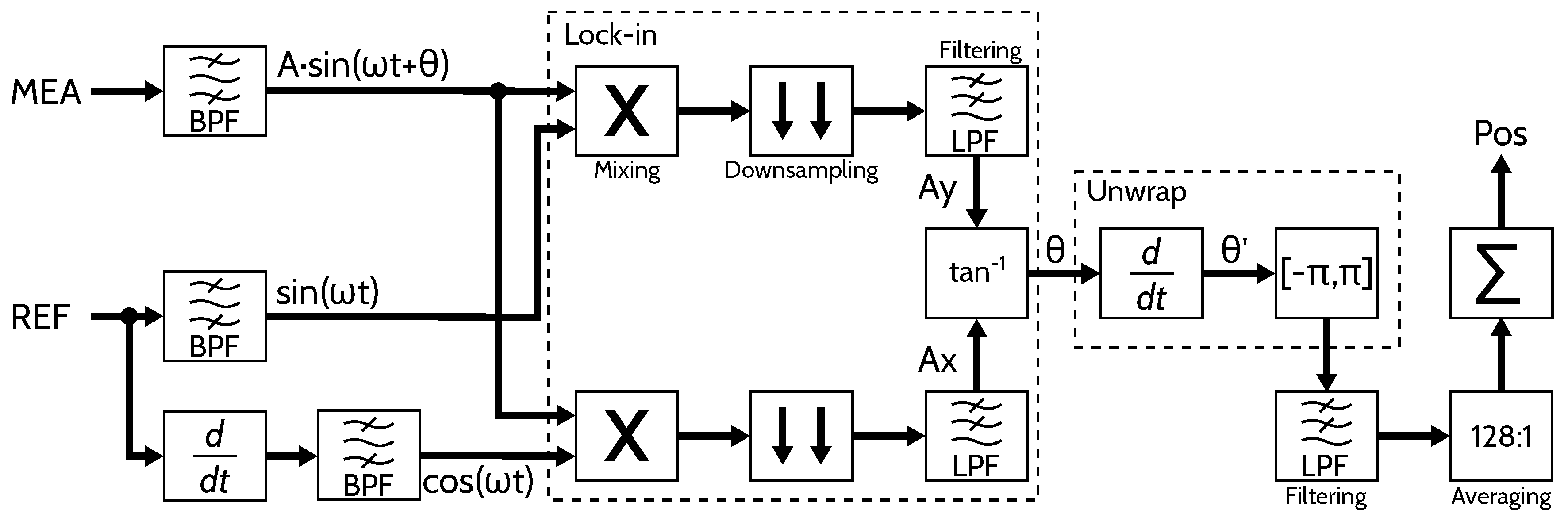
Figure 2.
Method simulation with reference and measurement signals at 2.7 MHz, a) input signals coming from laser head and b) filtered and resulting angle ().
Figure 2.
Method simulation with reference and measurement signals at 2.7 MHz, a) input signals coming from laser head and b) filtered and resulting angle ().
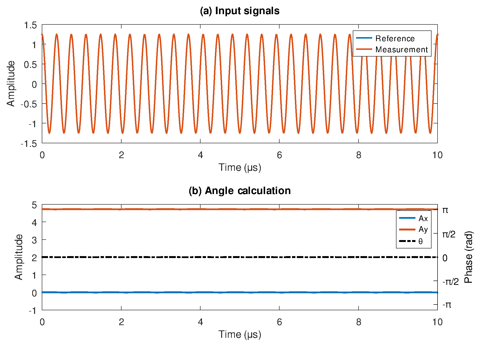
Figure 3.
Simulation with a reference signal at 2.7 MHz and a measurement signal 200KHz below, a) input signals coming from laser head and b) filtered and resulting angle ().
Figure 3.
Simulation with a reference signal at 2.7 MHz and a measurement signal 200KHz below, a) input signals coming from laser head and b) filtered and resulting angle ().
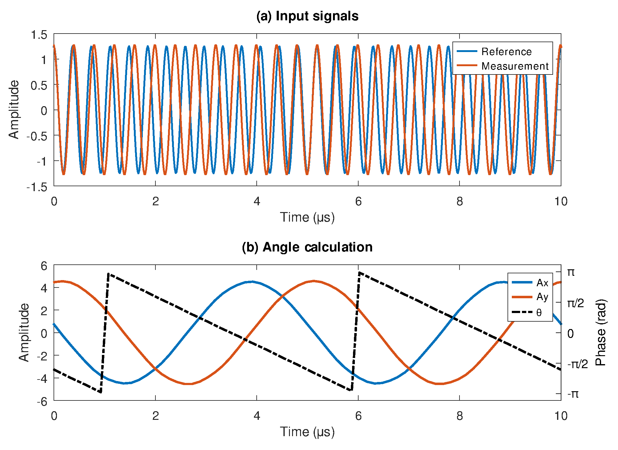
Figure 4.
Simulation with a reference signal at 2.7 MHz and a measurement signal 500KHz above, a) input signals coming from laser head and b) filtered and resulting angle ().
Figure 4.
Simulation with a reference signal at 2.7 MHz and a measurement signal 500KHz above, a) input signals coming from laser head and b) filtered and resulting angle ().
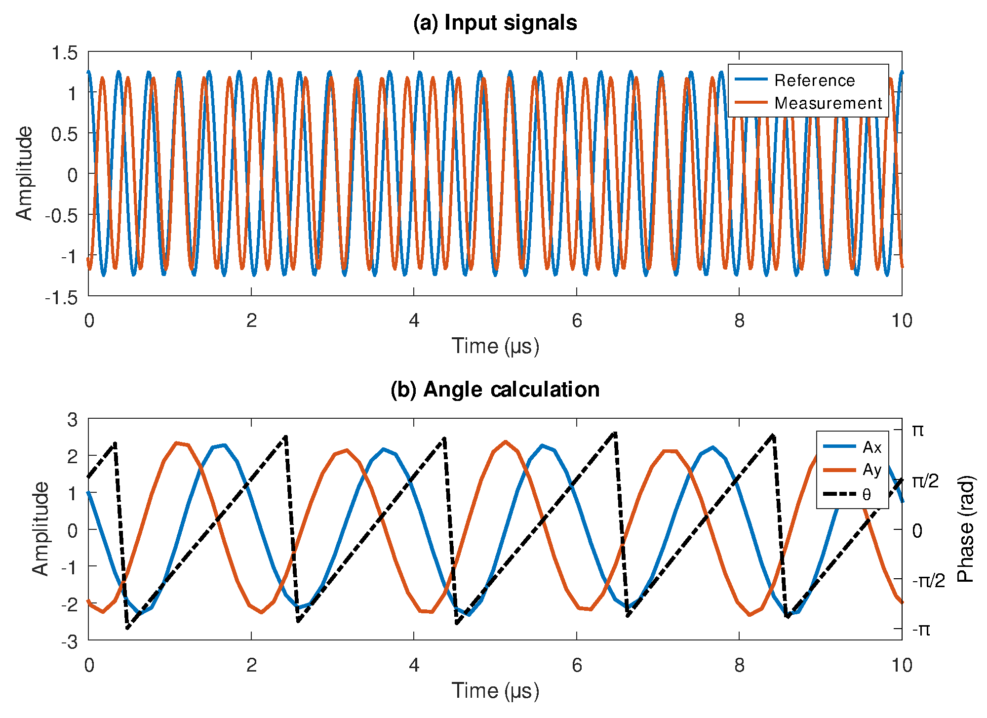
Figure 5.
Raw and filtered phase obtained by the lock-in in a zero-motion interferometer signal.

Figure 6.
Real-world signals from a heterodyne laser head, a) full captured signals and b) 5 s detail.
Figure 6.
Real-world signals from a heterodyne laser head, a) full captured signals and b) 5 s detail.
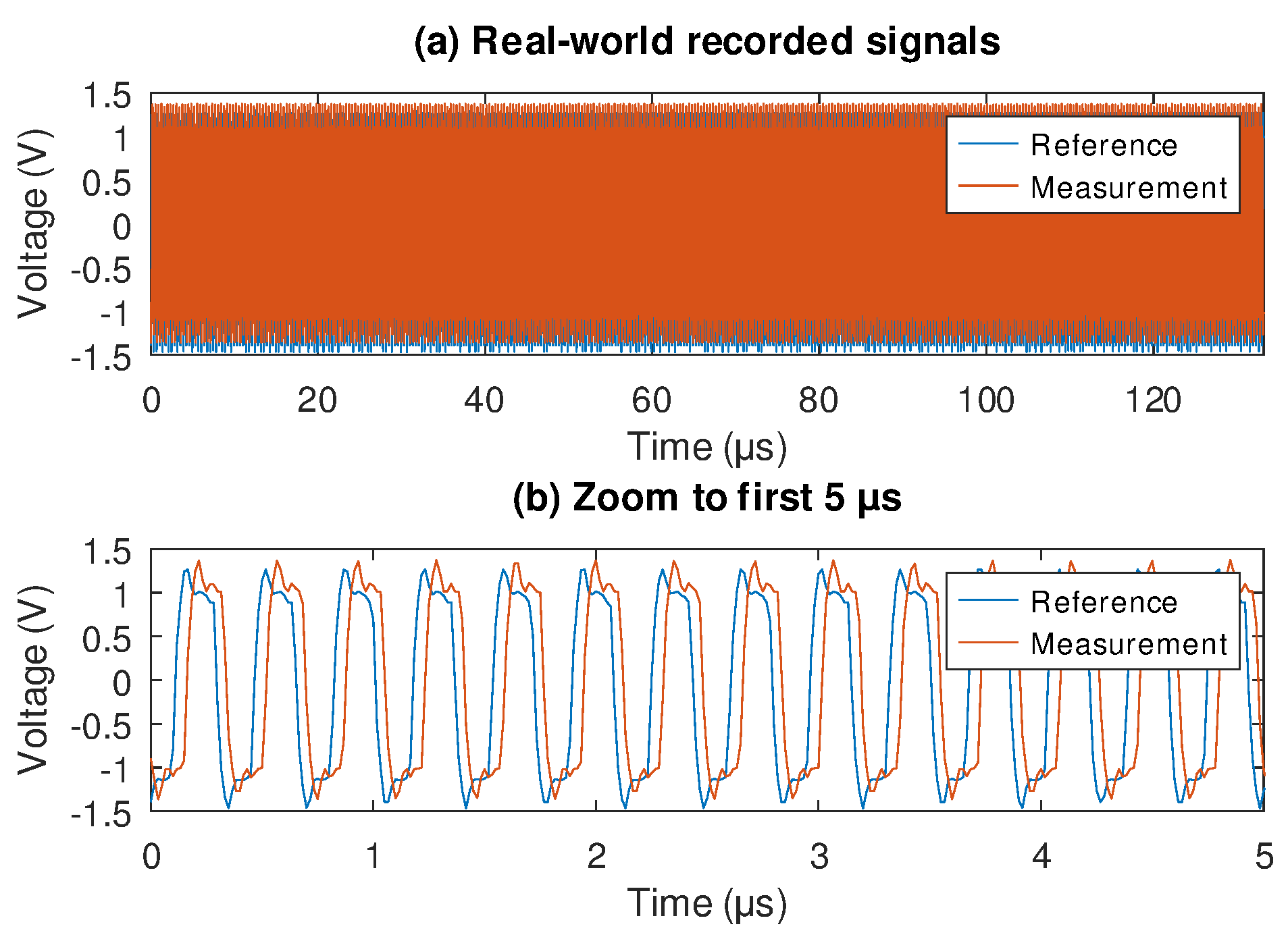
Figure 7.
Phase measurement in real-world signals, a) original signals, b) filtered input signals, and c) phase result obtained with the LDPD method.
Figure 7.
Phase measurement in real-world signals, a) original signals, b) filtered input signals, and c) phase result obtained with the LDPD method.
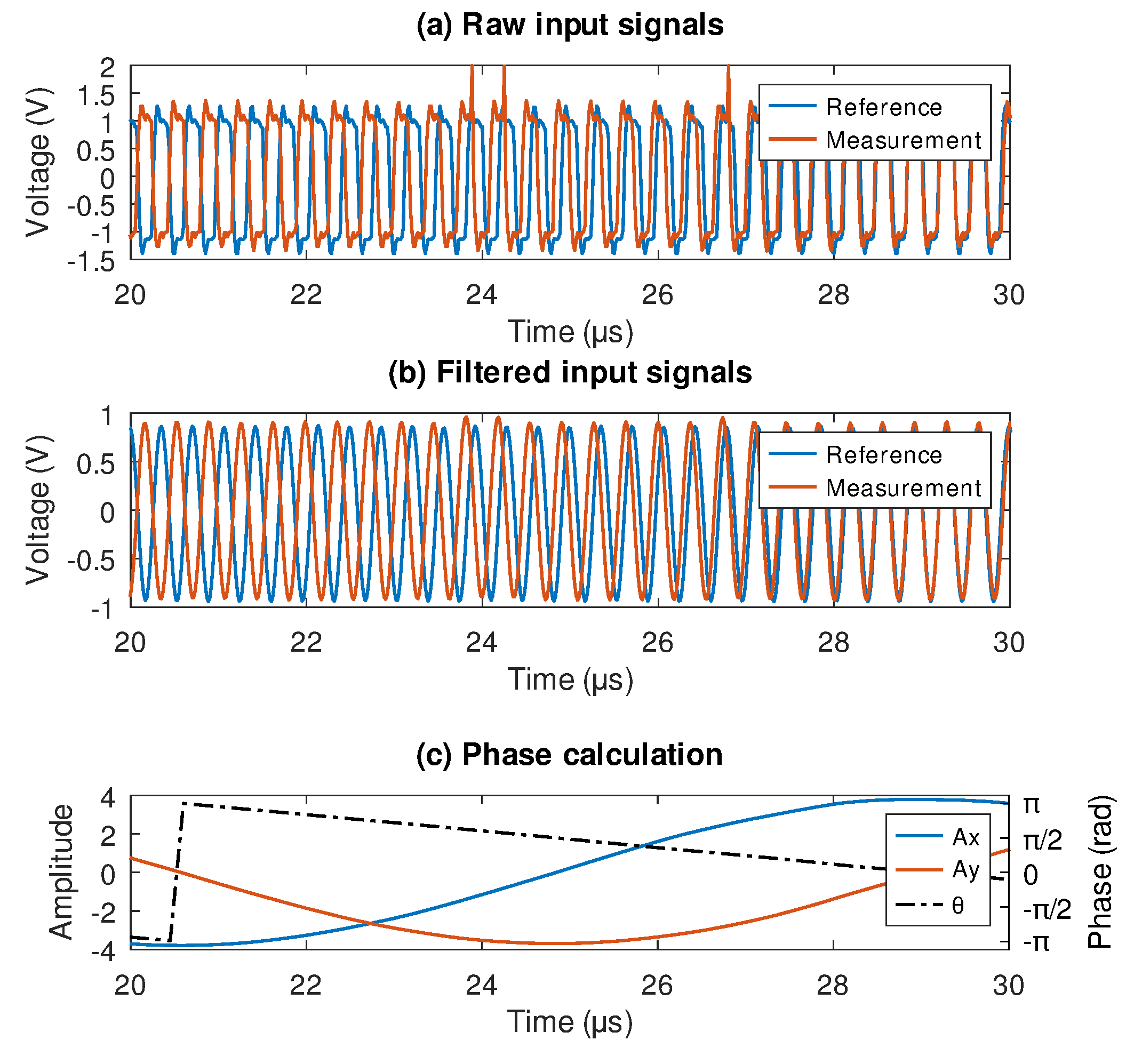
Figure 8.
Block diagram for the LDPD method hardware implementation based on FPGA.
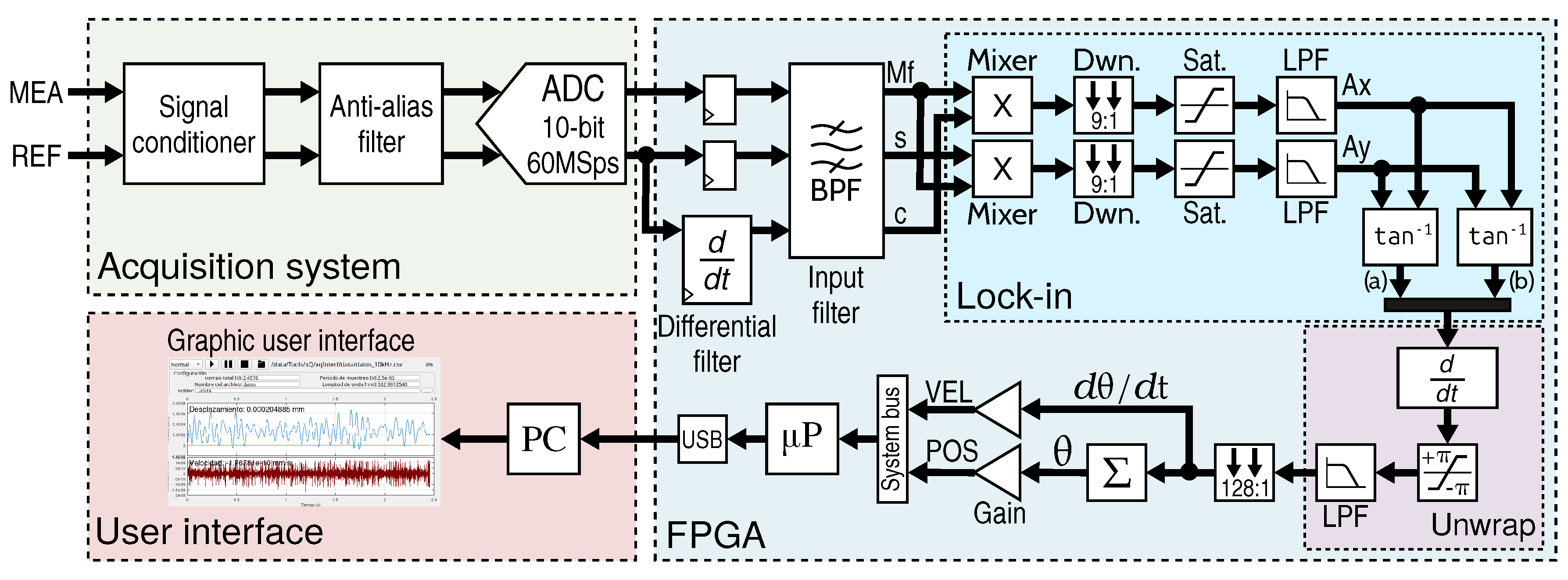
Figure 9.
Parallel FIR filter structure used to implement BPF and LPF filters.
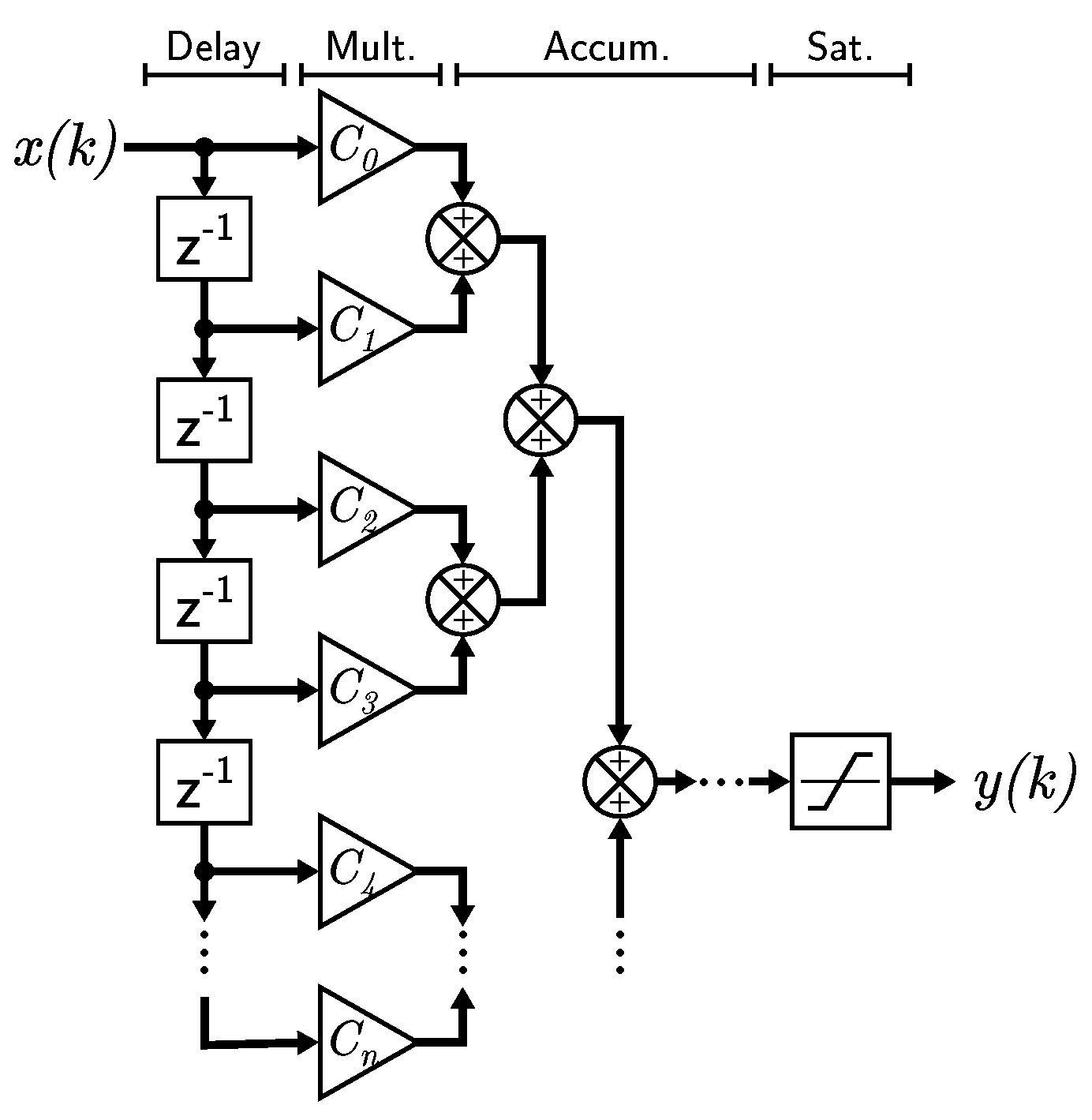
Figure 10.
Developed FPGA board and FPGA resource use: (a) Custom-designed FPGA board and acquisition system (LIFIUAQ). (b) FPGA resource utilization as reported by the AMD Vivado Post-Implementation tool.
Figure 10.
Developed FPGA board and FPGA resource use: (a) Custom-designed FPGA board and acquisition system (LIFIUAQ). (b) FPGA resource utilization as reported by the AMD Vivado Post-Implementation tool.
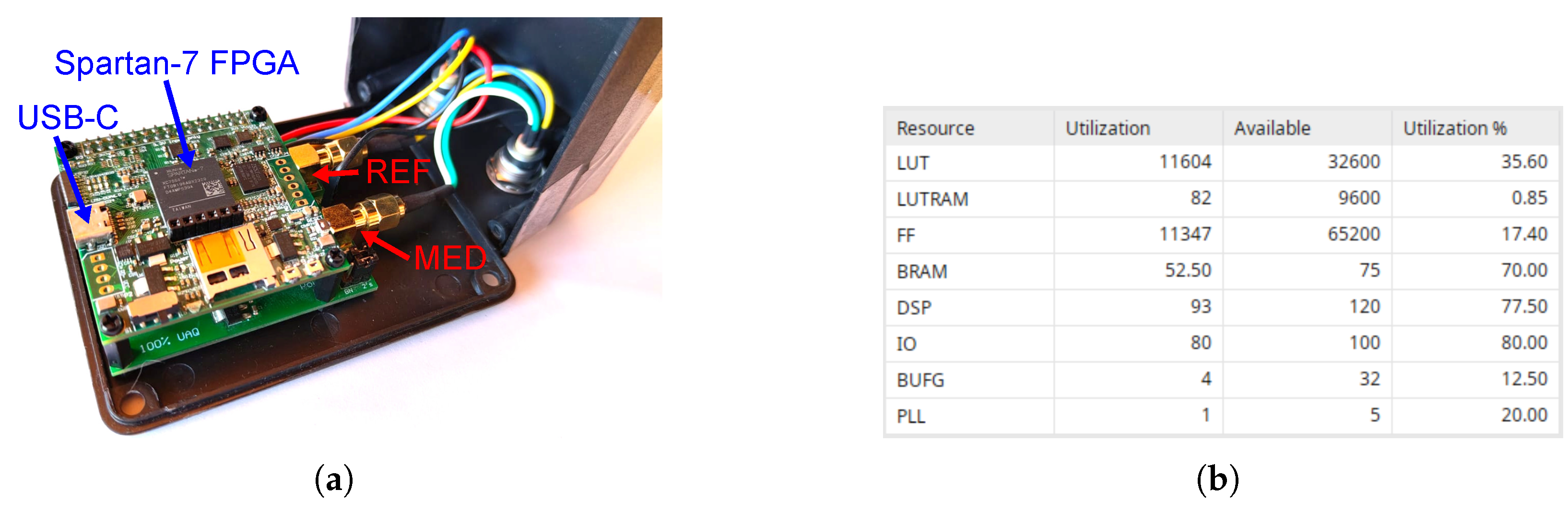
Figure 11.
Zero movement test a) using a function generator and b) from the heterodyne laser head.
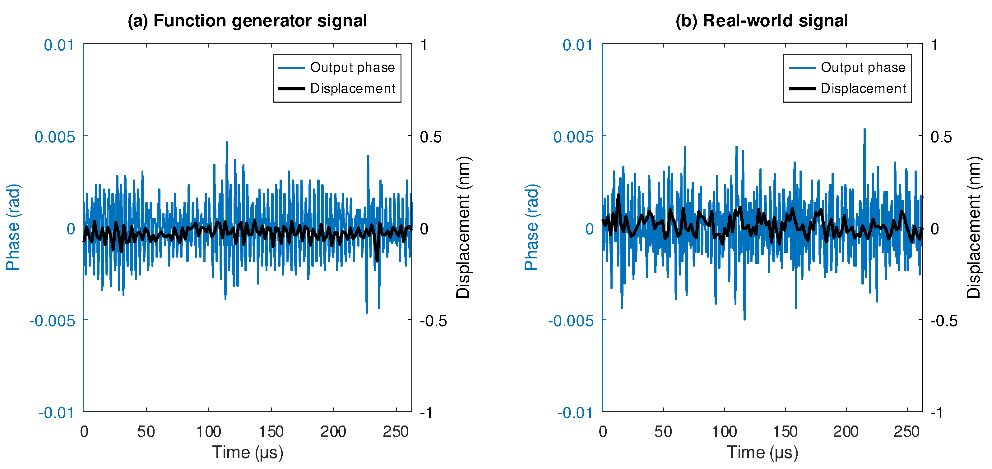
Figure 12.
Statistical comparison between function generator and real-wold tests.
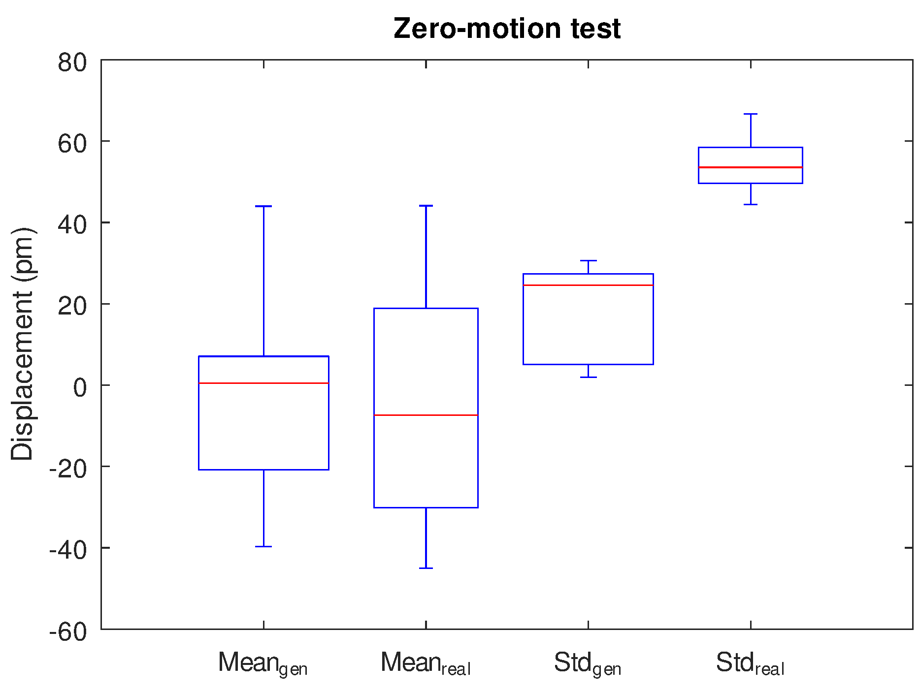
Figure 13.
Experimental setup for the moving target test, showing the principal components: laser heads, moving mirror, beam splitter, FPGA processing system (LIFIUAQ), and host PC.
Figure 13.
Experimental setup for the moving target test, showing the principal components: laser heads, moving mirror, beam splitter, FPGA processing system (LIFIUAQ), and host PC.
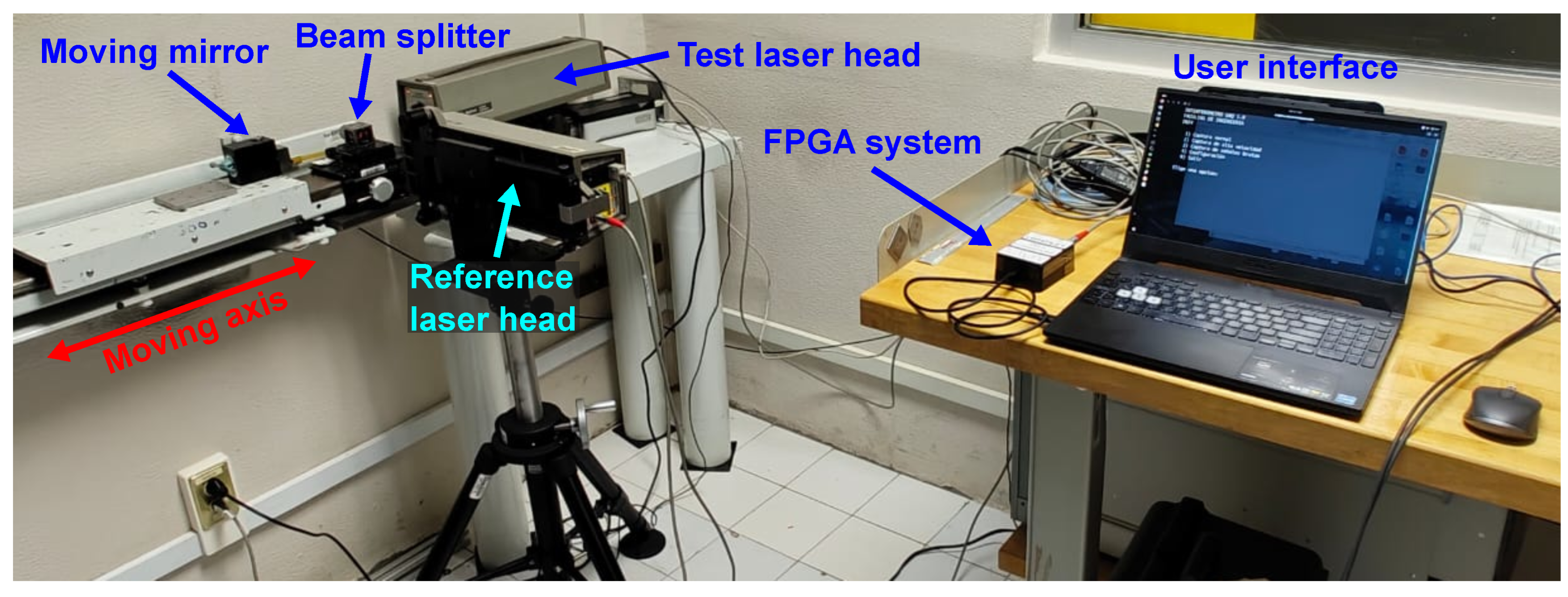
Figure 14.
Forward and backward path for the in-motion scenario test.
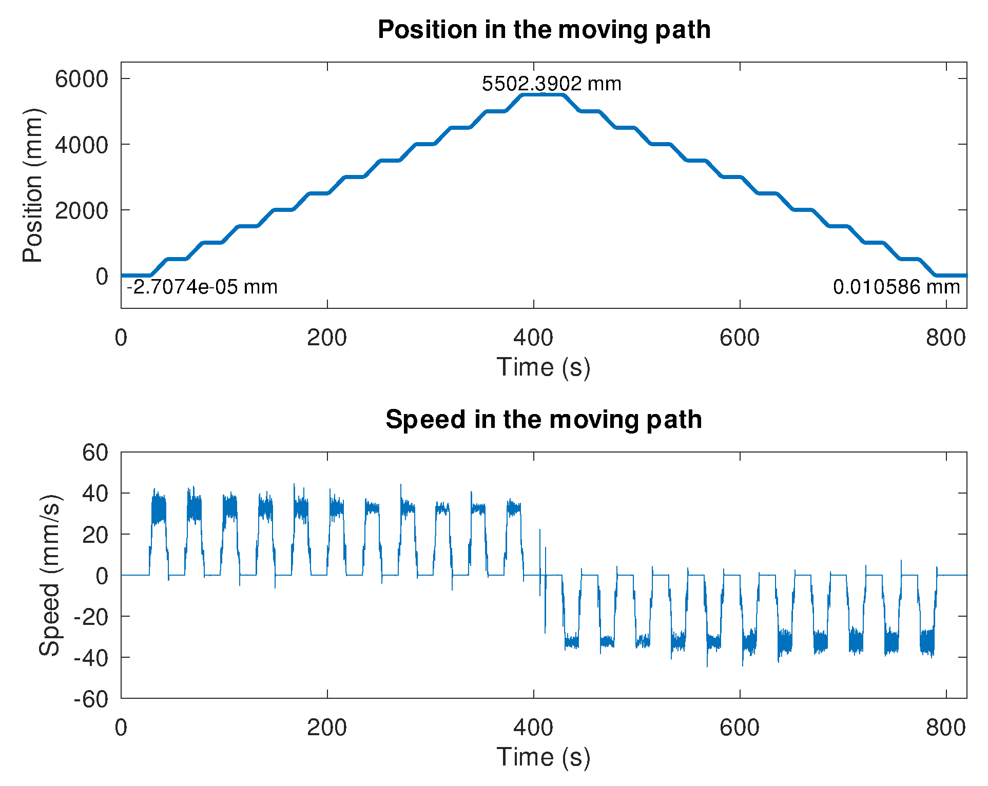
Figure 15.
Transient and steady state responses: (a) Transient capture on every motion step. (b)7-second window at the end of the motion step stop.
Figure 15.
Transient and steady state responses: (a) Transient capture on every motion step. (b)7-second window at the end of the motion step stop.
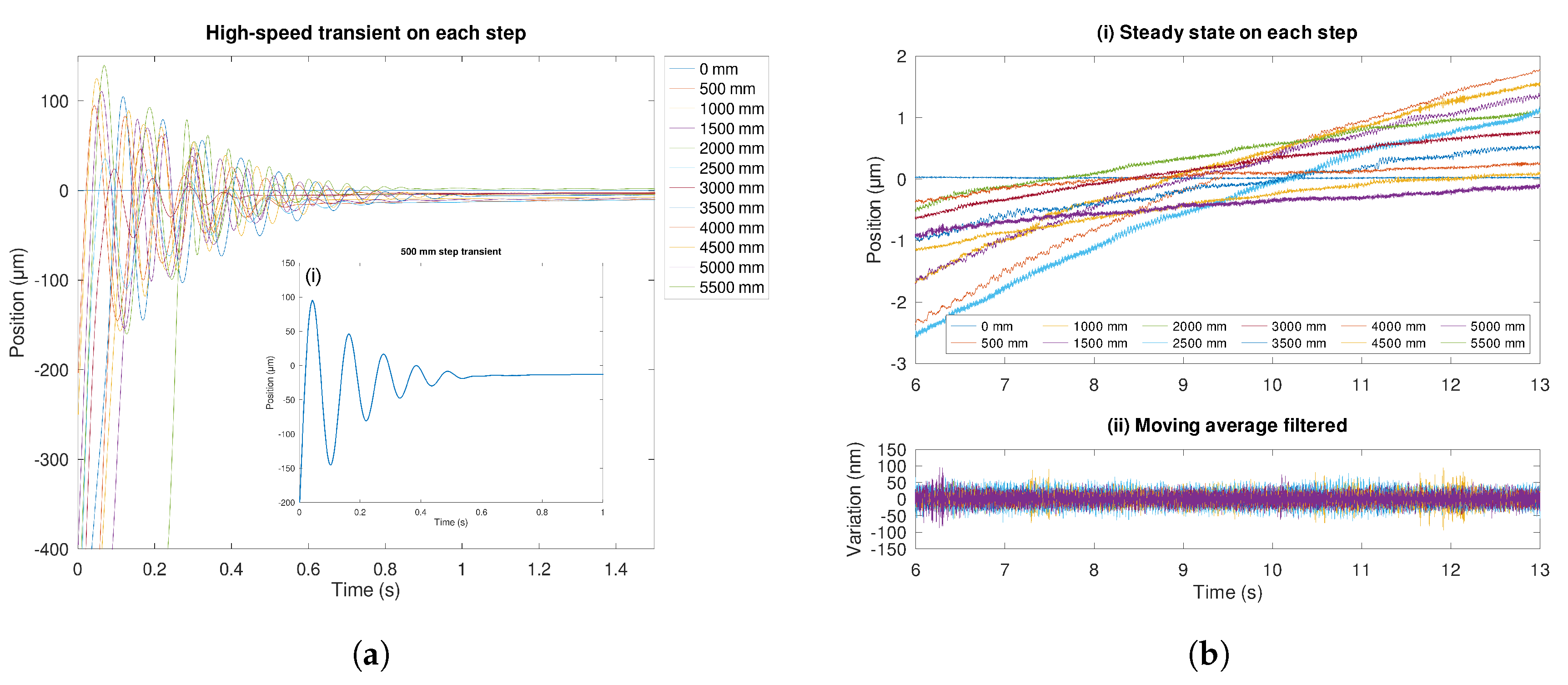

Table 1.
White noise simulation results.
| SNR | Phase (rad) | Displacement (nm) | ||
| Mean | Std. Dev. | Mean | Std. Dev. | |
| w/o N. | 0.003 | 0.010 | 0.382 | 0.001 |
| 60 dB | 0.012 | 0.150 | 1.279 | 0.015 |
| 50 dB | 0.019 | 0.490 | 1.984 | 0.049 |
| 40 dB | -0.149 | 1.549 | -0.015 | 0.156 |
| 20 dB | 0.704 | 15.615 | 0.071 | 1.573 |
Table 2.
Measurement comparison between reference system and proposed system.
| Stop | Step position (mm) | CENAM measure (m) | LIFIUAQ measure (m) | Error (nm) | Resolution (nm) |
|---|---|---|---|---|---|
| 1 | 0 | -0.03 | -0.01 | 22.08 | 7.08 |
| 2 | 500 | 214.11 | 213.75 | 357.74 | 10.03 |
| 3 | 1000 | 253.36 | 253.27 | 90.19 | 20.71 |
| 4 | 1500 | 402.81 | 402.63 | 177.60 | 17.06 |
| 5 | 2000 | 500.44 | 500.72 | -280.55 | 14.45 |
| 6 | 2500 | 566.83 | 566.08 | 745.84 | 26.63 |
| 7 | 3000 | 702.42 | 702.48 | -63.20 | 14.39 |
| 8 | 3500 | 753.93 | 753.67 | 250.18 | 15.04 |
| 9 | 4000 | 903.25 | 903.22 | 26.82 | 11.97 |
| 10 | 4500 | 989.49 | 988.98 | 508.15 | 15.42 |
| 11 | 5000 | 1206.71 | 1206.20 | 507.72 | 19.90 |
| 12 | 5500 | 2392.45 | 2393.00 | -559.41 | 13.97 |
Disclaimer/Publisher’s Note: The statements, opinions and data contained in all publications are solely those of the individual author(s) and contributor(s) and not of MDPI and/or the editor(s). MDPI and/or the editor(s) disclaim responsibility for any injury to people or property resulting from any ideas, methods, instructions or products referred to in the content. |
© 2025 by the authors. Licensee MDPI, Basel, Switzerland. This article is an open access article distributed under the terms and conditions of the Creative Commons Attribution (CC BY) license (http://creativecommons.org/licenses/by/4.0/).
Copyright: This open access article is published under a Creative Commons CC BY 4.0 license, which permit the free download, distribution, and reuse, provided that the author and preprint are cited in any reuse.


