Submitted:
09 February 2025
Posted:
10 February 2025
Read the latest preprint version here
Abstract
Starting from earthquake fault dynamic equations, a correspondence between earthquake occurrence statistics in a seismic region before a major earthquake and the statistics of solutions to a nonlinear eigenvalue problem whose eigenfunctions characterize the seismic velocity model of the region is presented. Modelling the eigenvalue solution statistics with a 2D Coulomb gas statistical physics model, previously reported deviation of seismic activation earthquake occurence statistics from Gutenberg-Richter statistics in time intervals preceding a major earthquake is derived. It is also explained how statistical physics modelling predicts a finite dimensional nonlinear dynamic system describes rupture nucleation in the seismic activation region, and how this prediction can be tested experimentally.
Keywords:
seismic activation
; statistical physics
; geodynamics
; signal processing
1. Introduction
An increase in the number of intermediate sized earthquakes () in a seismic region preceding the occurrence of an earthquake with magnitude , referred to as seismic activation, has been observed to occur Bowman et al. (1998). For example, seismic activation was observed in a geographic region spanning for a period of time between 1991 and 1999 preceding the magnitude 7.6 Chi-Chi earthquake Chen (2003). Figure 1 shows a schematic plot of the cumulative distribution of earthquakes of different magnitudes in a region undergoing seismic activation in two different time intervals of equal duration preceding occurrence of a major () earthquake at time . In this figure, is a real time parameter, and is the characteristic time of major earthquake recurrence assuming an earthquake of similar magnitude occurred in the same region at Rundle et al. (2001); Vallianatos and Sammnds (2004). Importantly, the cumulative distribution of earthquakes in a time interval of fixed width increasingly deviates away from a Gutenberg-Richter linear log-magnitude plot as the end of the time interval approaches .
As a means of predicting the time at which a major earthquake preceded by seismic activation occurs, it has been hypothesized that the average seismic moment of earthquakes occuring in intervals of time preceding a major earthquake obeys an inverse power of remaining time to failure law:
and that as a result, the cumulative Benioff strain , defined as:
where is the seismic moment of the earthquake in the region starting from a time preceding the major earthquake, and is the number of earthquakes occurring in the region up to time , satisfies Tzanis et al. (2000):
Notably, the exponent selection of in equation (2) is not necessary to derive formula (3) with a different arithmetic relation between and , but appears to have been commonly selected by previous researchers based on resulting predictions of major earthquake occurrence time when formula (3) is fit to real seismic data Vallianatos and Chatzopoulos (2018). It is also noted that when a fit to real seismic data is performed, a value is typical Bowman et al. (1998).
A mathematical model of seismic activation based on damage mechanics of earthquake faults has been put forth to derive equation (3) with a value Ben-Zion and Lyakhovsky (2002). In this derivation, the occurrence of seismic activation earthquakes progressively decreases the average shear modulus of fault material in the seismic region where subsequent seismic activation earthquakes occur, and the result is determined by a Boltzman kinetic type description of how ruptured faults of different lengths at different positional locations grow and join together Tzanis and Vallianatos (2003).
In addition to the damage mechanics model of seismic activation, an empirical model of seismic activation using statistical physics known as the Critical Point (CP) model has been put forth to derive equation (3) with a value Rundle et al. (2001). In this derivation, the inverse power of remaining time to failure law:
is asserted based on identifying the mean rupture length of earthquakes occuring at time with the correlation length of a statistical physical system described by Ginzburg-Landau mean field theory with a temperature parameter depending on , whereby:
and relation (4) follows from the scaling relation which holds when the fault material shear modulus is constant in the seismic activation region Rundle et al. (2003). Importantly, previous work has not explained why it is physically reasonable to describe statistics of seismic activation with thermal equilibrium statistical physics formalism, or what predictions other than time of major earthquake occurrence are possible with such models Newman et al. (1995). Therefore, the objective of this article is to advance the detailed mathematical description of the correspondence between nonlinear differential equation modelling and statistical physics modelling of seismic activation in a way that advances testing of model predictions against real seismic measurements.
The outline of the article is as follows. Section 2 introduces a sine-Gordon equation modelling earthquake fault dynamics during seismic activation and explains how inverse scattering theory of this equation implies a relation between solutions to a nonlinear eigenvalue problem whose eigenfunctions characterize the seismic velocity model of the region and statistical physics. Section 3 explains how statistics of the eigenvalue solutions are related to earthquake occurrence statistics, and how describing these statistics with a 2D Coulomb gas statistical physics model accounts for deviation of earthquake occurrence statistics from Gutenberg-Richter statistics before a major earthquake. Section 4 concludes by commenting on how statistical physical modelling implies the phase space dimension of a nonlinear dynamical system characterizing rupture nucleation in the seismic activation region is finite, and how this implication can be tested against real seismic measurements.
2. Methods
2.1. 1D Fault Dynamics Inverse Scattering Theory
In 1+1 spacetime dimensions, the differential equation:
has been used to model migration of earthquake hypocentres along earthquake faults in seismic regions over periods of time during which multiple earthquakes occur Bykov (2001). In this equation, is real time, z coordinates a direction of earthquake hypocenter migration along an earthquake fault, is the local displacement of elastic material across the earthquake fault, is the local inertial force acting on the fault material, is the local elastic restoring force acting on the fault material, and and are local frictional force acting on the fault material attributed to periodic contact of the material with tectonic plates on either side of the fault. If the earthquake fault material has constant height h and shear modulus along the fault, a soliton (2 kink) solution to equation (6) can be interpreted to describe growth of an interval where earthquake rupture has occurred along the z-axis, which in this 1 dimensional model is identified with the both the direction of hypocentre migration and the direction of all earthquake slip vectors Carlson et al. (1994).
Restricting focus to the case , with rescaling of , z, and , each of the constants A, B, and D in equation (5) can be set to 1. With this rescaling, and definition of the matrices:
for an arbitary complex number , the equation:
is equivalent to equation (5) Khan (2020). Introduction of the matrix operator also permits introduction of the associated seismic wave scattering problem:
in which is an auxillary parameter, and oscillatory dependence of the incoming and outgoing scattered waves on a scattering time parameter t has been implicitly assumed in the definitions of and . According to the inverse scattering method, the importance of the operator is that it determines real time evolution of scattering data determined by the operator .
Upon definition of scattering problem (10), the inverse scattering method proceeds by determining an infinite set of its left and right scattering (i.e. Jost) solutions and , indexed by complex wave numbers , with asymptotics Aktosun et al. (2010):
and:
Next, using equation (9), real time evolution of the Jost functions is calculated in terms of -variation of the reflection coefficients and a finite set of complex numbers associated with complex wave numbers of bound state solutions to linear system (10). Finally, the real time evolved sine-Gordon equation solution is determined by applying an inverse scattering transform to the real time evolved scattering data as indicated in Figure 2. Note that according to 1D scattering theory, scattering bound states are in correspondence with zeroes of the function , while resonant scattering states are in correspondence with zeros of the reflection coefficients and at fixed values of . Also note that in general the bound and resonant state values have non-zero imaginary components, and are located symmetrically with respect to the imaginary axis in the complex -plane.
To clarify the physical relation between scattering data used by the inverse scattering method and seismic activation physics, consider the simpler 1D scattering problem in which a scattering potential function is compactly supported along the z-axis, and the operator:
has infinitely many resonant state eigenfunctions satisfying the elastic wave equation:
and finitely many bound state eigenfunctions with negative real eigenvalues . In this situation, the Jost eigenfunctions of operator (16) define a spectral kernel whose determinant equates to the potential V, which in a 1D scattering context implies the Jost functions define the velocity model of the 1D elastic wave equation Dyson (1976). Based on this established mathematical result, it is conjectured that the scattering potential function also equates to a determinant of an operator defined by Jost functions of scattering problem (10).
To clarify the physical relation between inverse scattering theory bound states and seismic activation it is noted that a solution to the linear seismic wave equation:
in which the auxillary seismic wave scattering time parameter t is introduced and tracks scattering potential changes associated with seismic activation, and for which and are compactly supported, has a resonant scattering expansion of the form Bindel and Zworski (2007):
in the limit . In this expansion, bound state eigenfunctions determine characteristic length scales at which unstable growth of fault material displacement may occur across the earthquake fault. Based on this interpretation, it is hereby suggested that inverse scattering thery bound states describe patterns of stress distribution in unruptured material as fault ruptures grow and nucleate.
For example, if is a potential well of depth which is independent of , nonzero for , and zero elsewhere, there exist finitely many bound state eigenfunctions which decay exponentially with increasing :
for a discrete set of spatial decay constants:
whose inverse values determine characteristic length scales at which unstable growth of fault material displacement may occur across the earthquake fault. Figure 3 shows a plot of resonant and bound state frequency locations for three situations in which is a square well potential of increasing width and fixed height.
2.2. 3D Fault Dynamics to Statistical Physics
To generalize the previous discussion of inverse scattering theory in 1 spatial dimension to 3 spatial dimensions, suppose a major earthquake hypocentre resides in an elastic half space in such a way that the elastic parameters of the half space are constant outside a sphere of diamater centred at the hypocentre. Moreover, suppose that with appropriate definition of a perfectly matched layer at the sphere’s boundary, dependent on complex frequency, elastic scattering resonant frequencies at time are determined by solution to a nonlinear eigenvalue problem whose solutions satisfy an equation Bindel (2006):
With this supposition, the complex resonant frequency set constitutes a 3D generalization of inverse scattering data that depends on , and whose real time evolution is necessarily in correspondence with real time evolution of the half space elastic parameters.
Importantly, the discussion in the previous paragraph suggests that rather than being a set of continuously changing values, the resonant frequency set is discontinuously updated with occurrence of each seismic activation earthquake, whereby a frequency is removed from the set and other frequencies in the set are affected by alteration of the fault rupture pattern, as illustrated in Figure 4 Lei and Sornette (2022). For this reason, rather than describing the resonant frequency set deterministically, it is now put forth that this set be described probabilistically by defining a resonant frequency probability density that depends on time. More specifically, it is suggested that the resonant frequency condition be interpreted as an eigenvalue condition on a matrix selected from a -dependent ensemble of random matrices. From this point of view, varying the real time parameter varies the statistical distribution of the random matrices, and in accordance with original statistical physics models of seismic activation, these random matrix models may be related by renormalization group flow Saleur et al. (1996).
3. Results
To relate the discussion in the previous chapter to seismic activation earthquake occurrence statistics, first define and as the corner frequency and rupture length of the largest seismic activation earthquake occurring before time . From this definition, the observed scaling relation between earthquake corner frequency and seismic moment :
together with the scaling relation:
imply Aki (1967):
Next, suppose that the eigenfunction of a solution to defines a lithospheric stress distribution preceding a seismic activation earthquake of rupture length , and that the probability of this earthquake occurring the time interval is proportional to , where is the quality factor of the lithospheric resonance at frequency . Then, if is the density of nonlinear eigenvalue solutions in the interval , the number of earthquakes with corner frequency less than or equal to occurring during the time interval is:
To specify the mathematical form of the integral in equation (25), recall that the Gutenberg-Richter law implies the total number of earthquakes of Richter magnitude in the interval occurring in the seismic activation region in the time interval is proportional to:
which according to the relation:
between Richter magnitude and seismic moment satisfies:
Therefore, assuming the Gutenberg-Richter law is valid, it follows that:
To account for modification to the Gutenberg-Richter law in time intervals preceding a major earthquake using statistical physics, it is now conjectured that for earthquake corner frequencies:
the quantity describes the density of a 2D Coulomb gas in the vicinity of a test charge located at , whereby Goldenfeld (1992):
for equal to the lowest corner frequency of a seismic activation earthquake preceding the major earthquake. With this conjecture, equation (25), modified to account for occurrence of an earthquake at corner frequency , implies:
which in turn implies the logarithm:
when plotted against Richter magnitude for , can have either of the cumulative distribution curve shapes shown in Figure 1 for different time intervals, depending on the value of .
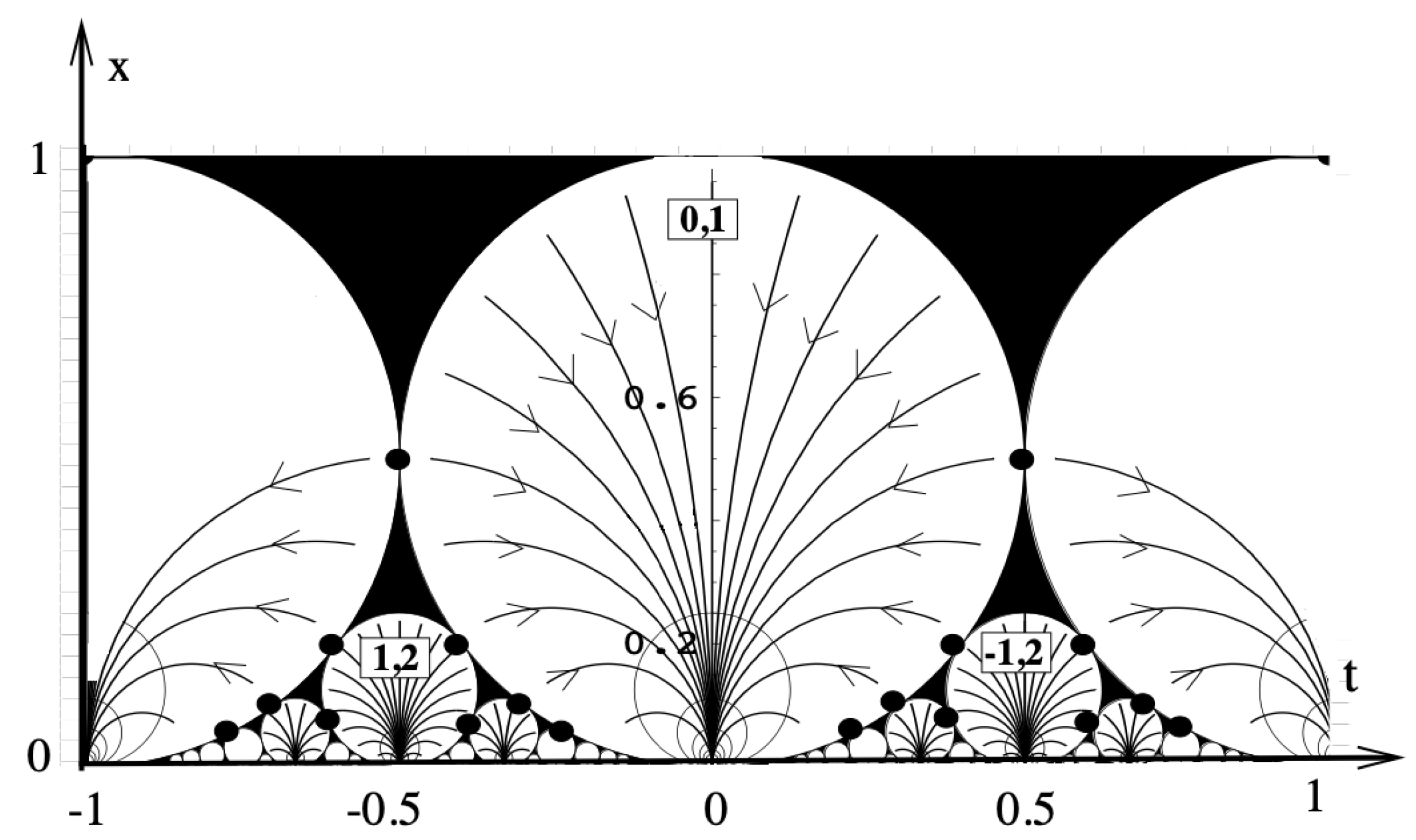
Having conjectured 2D Coulomb gas statistical physics are relevant to accounting for deviation of earthquake occurrence statistics from Gutenberg-Richter statistics during seismic activation, it is now further conjectured, in accordance with previous statistical physics models of seismic activation, that , where is a parameter in a -dependent 2D sine Gordon statistical physics model whose parameters at different values of are related by renormalization group flow Balog et al. (2018); Carpentier (1999). With this additional conjecture, an increase in the value of as accounts for increasing steepness of the cumulative distribution curve shown in Figure 1. A phase diagram of a 2D sine Gordon model with a renormalization group flow indicated by arrows is shown in Figure 5. In this diagram, different vaues of the flow coordinate `t’ equate to at different values of in such a way that is the horizontal coordinate of a point of tangency between two of the Ford circles. It is noted that this phase diagram corresponds to the description of a more general 2D sine Gordon statistical physics model defined by a field theory with fields Dubrovin and Yang; (2020) Varchenko (1990); Zabrodin (2010).
4. Discussion
Previous work has identified predicting the time of occurrence of major earthquakes as a possible application of statistical physics models of seismic activation, but this application has not yet been realized Bowman et al. (1998). In more recent times, earthquake early warning algorithms such as FinDer and Virtual Seismologist have been developed which can in principle use previous earthquake occurrence statistics as input, and most recently, artificial intelligence algorithms such as QuakeGPT have been developed for predicting the occurrence of major earthquakes using seismic event records created with stochastic simulators as training data Böse et al. (2023); Rundle et al. (2024). Therefore, a practical applied science goal for the statistical physics model presented in this article appears to be improving the predictive performance of one or more of these existing earthquake early warning algorithms by appropriately modifying their earthquake occurrence statistical inputs, acknowledging that preliminary tests of the model’s validity against real seismic data must be passed before achieving this application objective can be considered a realistic possibility.
From a geophysical testing point of view, if it is true that the growth of unstable stress modes within the Earth during seismic activation are determined by statistical physics renormalization group flow mathematics, and, as a result, a nonlinear dynamical system of phase space dimension N characterizes the nucleation of shear stress in a seismic region preceding a major earthquake, a geophysical signal processing technique known as singular spectrum analysis should apply to determine this phase space dimension Broomhead and King (1986). Therefore, it is suggested that coda wave interferometry measurements of relative changes in seismic surface wave and/or body wave velocity be performed between pairs of seismic stations in a seismic region over a duration of time during which seismic activation is known to have occurred, and used as input to a time domain multichannel singular spectrum analysis algorithm Merrill et al. (2023). The number of channels of this algorithm would equate to the number of station pairs, and the number of singular values output by the algorithm in different time windows preceding occurrence of a major earthquake should provide some indication of a finite value for N if the statistical physics model of seismic activation is correct in principle. With reference to previous geophysical application of singular spectrum analysis, performed in the frequency domain, the signal processing algorithm suggested here is different in that it should be carried out in the time domain rather than the frequency domain Sacchi (2009).
In conclusion, work towards improving current earthquake early warning systems can proceed in two directions. Firstly, as an initial check on whether or not the statistical physics modelling approach presented here could be of practical utility, work can be done to determine whether or not changes of the Earth’s elastic velocity model preceding major earthquakes, as determined by coda wave interferometry, can be processed to extract an integer identifiable as the phase space dimension of a nonlinear dynamical system. Secondly, work can be done to elaborate upon the statistical physics mathematical model of seismic activation presented in this article to determine other tests of its scientific validity and potential for practical application.
Acknowledgments
Thanks to my family for their support throughout completion of this research. Thanks to Dr. Girish Nivarti and Professor Richard Froese for their willingness to entertain discussions about the content of the article. The author declares they have no conflicts of interest.
References
- Akemann G, Mielke A, Pβler (2021) Spacing distribution in the 2D Coulomb gas: Surmise and symmetry classes of non-Hermitian random matrices at non-integer β.
- Aki K, 1967. Scaling law of seismic spectrum, J. geophys. Res., 72, 1217–1231. [CrossRef]
- Aktosun T, Demontis F, F Van der Mee C. Exact solutions to the sine-Gordon equation. Journal of Mathematical Physics. 51(12). [CrossRef]
- Balog I, Carpentier D, Fedorenko AA. Disorder-driven quantum transition in relativistic semimetals: functional renormalization via the porous medium equation. Physical review letters. 2018 121(16):166402. [CrossRef] [PubMed]
- Ben-Zion Y, Lyakhovsky V (2002) Accelerated seismic release and related aspects of seismicity patterns on earthquake faults. Earthquake processes: Physical modelling, numerical simulation and data analysis Part II :2385–2412.
- Bindel DS. Structured and parameter-dependent eigensolvers for simulation-based design of resonant MEMS (Doctoral dissertation, University of California, Berkeley).
- Bindel D, Zworski M. Symmetry of bound and antibound states in the semiclassical limit. Letters in Mathematical Physics. 2007 Aug;81:107–17. [CrossRef]
- Böse M, Andrews J, Hartog R, Felizardo C. Performance and next-generation development of the finite-fault rupture detector (FinDer) within the United States West Coast ShakeAlert warning system. Bulletin of the Seismological Society of America. 2023 Apr 1;113(2):648–63. [CrossRef]
- Bowman D, Ouillon G, Sammis C, Sornette A, Sornette D (1998) An observational test of the critical earthquake concept. Journal of Geophysical Research: Solid Earth 103(B10):24359–24372. [CrossRef]
- Broomhead D S, King G P (1986) Extracting qualitative dynamics from experimental data. Physica D: Nonlinear Phenomena 20(2-3):217–236. [CrossRef]
- Bykov V G (2001) Solitary waves on a crustal fault. Volcanology and Seismology 22(6):651–661.
- Carlson J M, Langer J S, Shaw B E (1994) Dynamics of earthquake faults. Reviews of Modern Physics 66(2):657. [CrossRef]
- Carpentier D (1999) Renormalization of modular invariant Coulomb gas and sine-Gordon theories, and the quantum Hall flow diagram. Journal of Physics A: Mathematical and General 32(21):3865. [CrossRef]
- Chen CC. Accelerating seismicity of moderate-size earthquakes before the 1999 Chi-Chi, Taiwan, earthquake: Testing time-prediction of the self-organizing spinodal model of earthquakes. Geophysical Journal International. 2003 155(1):F1-5. [CrossRef]
- Dubrovin B, Yang D (2020) Matrix resolvent and the discrete KdV hierarchy. Communications in Mathematical Physics 377:1823–1852. [CrossRef]
- Dyatlov S, Zworski M (2019) Mathematical theory of scattering resonances, volume 200. American Mathematical Soc.
- Dyson FJ. Fredholm determinants and inverse scattering problems. Communications in Mathematical Physics 47(2):171-83. [CrossRef]
- Dyson FJ, Mehta ML (1963) Statistical theory of the energy levels of complex systems. iv. Journal of Mathematical Physics 4(5):701–712. [CrossRef]
- Goldenfeld N. Lectures on phase transitions and the renormalization group. CRC Press; 2018.
- Hofstetter E, Schreiber M (1993) Statistical properties of the eigenvalue spectrum of the three-dimensional Anderson Hamiltonian. Physical Review B 48(23):16979. [CrossRef]
- Ito R, Kaneko Y (2023). Physical Mechanism for a Temporal Decrease of the Gutenberg-Richter b-Value Prior to a Large Earthquake. Journal of Geophysical Research: Solid Earth 128(12):e2023JB027413. [CrossRef]
- John S. Localization of light. Physics Today. 1991 May 1;44(5):32–40. [CrossRef]
- Khan BA, Chatterjee S, Sekh GA, Talukdar B (2020) Integrable systems: From the inverse spectral transform to zero curvature condition. arXiv preprint arXiv:2012.03456.
- Lei Q, Sornette D (2022) Anderson localization and reentrant delocalization of tensorial elastic waves in two-dimensional fractured media. Europhys. Letters 136(3): 1–7.
- Markos P (2006) Numerical analysis of the Anderson localization. arXiv preprint cond-mat/0609580.
- Merrill RJ, Bostock MG, Peacock SM, Chapman DS (2023) Optimal multichannel stretch factors for estimating changes in seismic velocity: Application to the 2012 Mw 7.8 Haida Gwaii earthquake. Bulletin of the Seismological Society of America 113(3):1077–1090. [CrossRef]
- Newman WI, Turcotte DL, Gabrielov AM (1995) Log-periodic behavior of a hierarchical failure model with applications to precursory seismic activation. Physical Review E 52(5):4827. [CrossRef] [PubMed]
- Rundle JB, Klein W, Turcotte DL, Malamud BD (2001) Precursory seismic activation and critical-point phenomena. Microscopic and Macroscopic Simulation: Towards Predictive Modelling of the Earthquake Process 2165–2182.
- Rundle JB, Turcotte DL, Shcherbakov R, Klein W, Sammis C (2003) Statistical physics approach to understanding the multiscale dynamics of earthquake fault systems. Reviews of Geophysics 41(4). [CrossRef]
- Rundle JB, Fox G, Donnellan A, Ludwig IG (2024) Nowcasting Earthquakes with QuakeGPT: Methods and First Results. arXiv e-prints. 2024 Jun:arXiv-2406.
- Sacchi M (2009) FX singular spectrum analysis. Cspg Cseg Cwls Convention 392–395.
- Saleur H, Sammis C, Sornette D (1996) Renormalization group theory of earthquakes. Nonlinear Processes in Geophysics 3(2):102–109. [CrossRef]
- Soerensen M, Schneider T (1991) Level-spacing statistics for the Anderson model in one and two dimensions. Physik B Condensed Matter 82(1):115–119. [CrossRef]
- Sornette D (1989) Acoustic waves in random media: II Coherent effects and strong disorder regime, Acustica 67(4):251–265.
- Tzanis A, Vallianatos F (2003) Distributed power-law seismicity changes and crustal deformation in the SW Hellenic ARC. Natural Hazards and Earth System Sciences 3(3/4):179–195. [CrossRef]
- Tzanis A, Vallianatos F, Makropoulos K (2000) Seismic and electrical precursors to the 17-1-1983, M7 Kefallinia earthquake, Greece: Signatures of a SOC system. Physics and Chemistry of the Earth, Part A: Solid Earth and Geodesy 25(3):281–7. [CrossRef]
- Vallianatos F, Chatzopoulos G (2018) A complexity view into the physics of the accelerating seismic release hypothesis: Theoretical principles. Entropy 20(10):754. [CrossRef] [PubMed]
- Vallianatos F, Sammonds P (2004) Evidence of non-extensive statistical physics of the lithospheric instability approaching the 2004 Sumatran–Andaman and 2011 Honshu mega-earthquakes. Tectonophysics 590:52–8. [CrossRef]
- Varchenko A (1990) Multidimensional hypergeometric functions in conformal field theory, algebraic K-theory, algebraic geometry. In Proceedings of the International Congress of Mathematicians 1:281–300.
- Wu RS, Aki K (1985) Scattering characteristics of elastic waves by an elastic heterogeneity. Geophysics 50(4):582–95. [CrossRef]
- Wu RS, Aki K (1988) Multiple scattering and energy transfer of seismic waves—Separation of scattering effect from intrinsic attenuation II. Application of the theory to Hindu Kush region. Scattering and Attenuations of Seismic Waves, Part I:49–80.
- Zabolotskaya EA, Ilinskii YA, Hay TA, Hamilton MF. Green’s functions for a volume source in an elastic half-space. The Journal of the Acoustical Society of America 131(3):1831–42. [CrossRef] [PubMed]
- Zabrodin A (2010) Canonical and grand canonical partition functions of Dyson gases as tau-functions of integrable hierarchies and their fermionic realization. Complex Analysis and Operator Theory 4:497–514. [CrossRef]
Figure 1.
Plot of the cumulative distribution of earthquakes of different magnitudes in a seismic zone in two different time intervals of equal width preceding occurrence of a major earthquake at Rundle et al. (2001); Vallianatos and Sammnds (2004).
Figure 1.
Plot of the cumulative distribution of earthquakes of different magnitudes in a seismic zone in two different time intervals of equal width preceding occurrence of a major earthquake at Rundle et al. (2001); Vallianatos and Sammnds (2004).

Figure 2.
Schematic diagram of inverse scattering method applied to solve the sine-Gordon equation Aktosun et al. (2010). Real time evolution of the scattering data determines a solution to the sine-Gordon equation upon application of an inverse scattering transform.
Figure 2.
Schematic diagram of inverse scattering method applied to solve the sine-Gordon equation Aktosun et al. (2010). Real time evolution of the scattering data determines a solution to the sine-Gordon equation upon application of an inverse scattering transform.
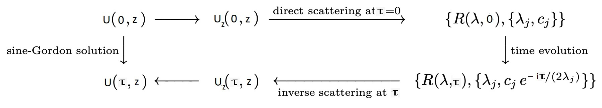
Figure 3.
Plots of resonant frequency and bound state frequency locations for 3 square well potentials of increasing width.
Figure 3.
Plots of resonant frequency and bound state frequency locations for 3 square well potentials of increasing width.
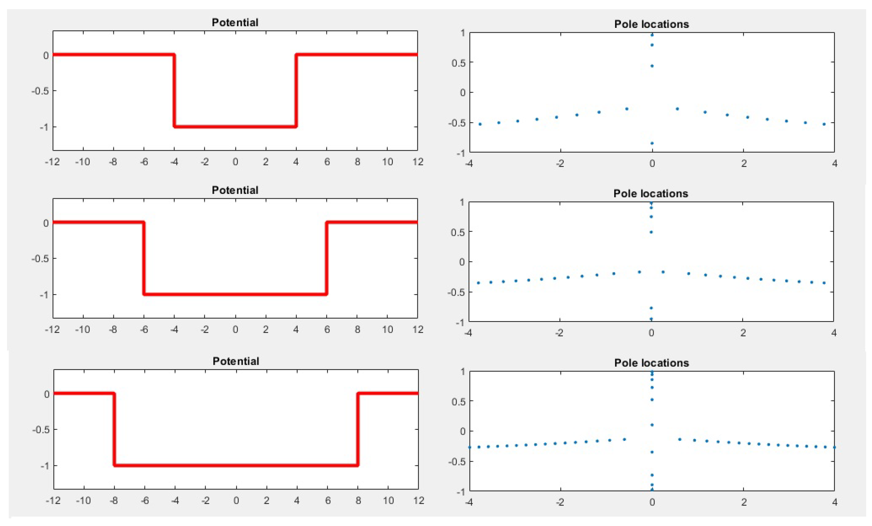
Figure 4.
Schematic illustration of seismic activation in a 2D geometry at four different times in which each black line represents an earthquake fault along which rupture has already occured, and the red line represents an earthquake fault along which shear stress is increasing prior to rupture Lei and Sornette (2022).
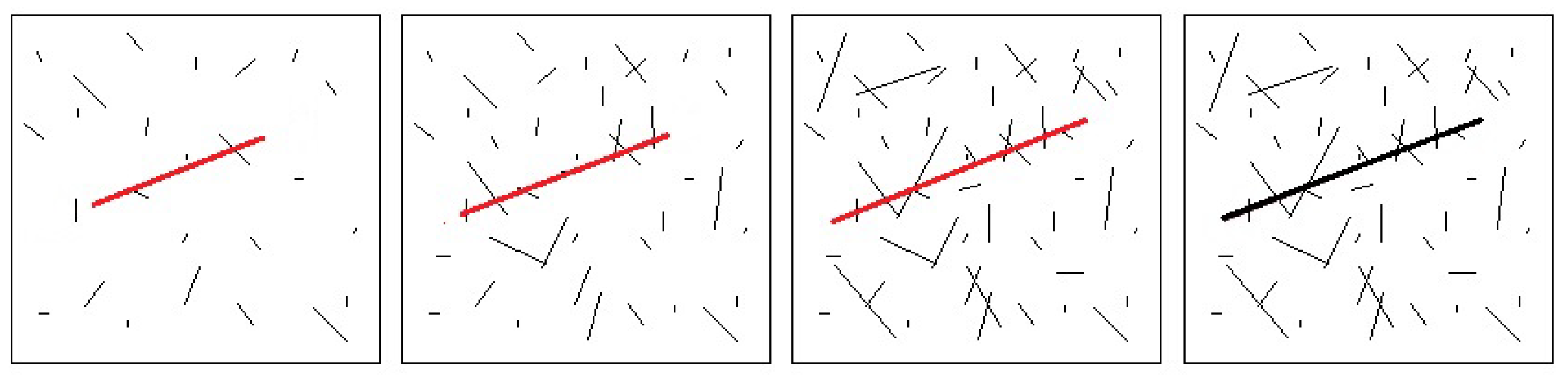
Figure 5.
Phase diagram of 2D sine Gordon statistical physics model with renormalization group flow indicated by arrows and KT critical points identified by circle tangencies Carpentier (1999).
Figure 5.
Phase diagram of 2D sine Gordon statistical physics model with renormalization group flow indicated by arrows and KT critical points identified by circle tangencies Carpentier (1999).
Disclaimer/Publisher’s Note: The statements, opinions and data contained in all publications are solely those of the individual author(s) and contributor(s) and not of MDPI and/or the editor(s). MDPI and/or the editor(s) disclaim responsibility for any injury to people or property resulting from any ideas, methods, instructions or products referred to in the content. |
© 2025 by the authors. Licensee MDPI, Basel, Switzerland. This article is an open access article distributed under the terms and conditions of the Creative Commons Attribution (CC BY) license (http://creativecommons.org/licenses/by/4.0/).
Copyright: This open access article is published under a Creative Commons CC BY 4.0 license, which permit the free download, distribution, and reuse, provided that the author and preprint are cited in any reuse.


