Submitted:
19 May 2025
Posted:
20 May 2025
You are already at the latest version
Abstract
Since 2001, after decades of a steady rate of magnitude ≥3 earthquakes in theUnited States, the annual number of earthquakes has increased exponentially fromapproximately 20 events per year in 2001 to up to 188 events per year in 2011.This increase is suspected to be human-induced. Modern physics tools, such asBayesian Data Analysis, can elucidate processes that trigger seismicity, both an-thropogenic and otherwise. This study introduces analytical methods and examinesanthropogenic processes, such as wastewater and CO2 injections, which can triggerseismicity. Statistical modeling of fluid injection and extraction has been enabledusing Bayesian inference. The San Andreas Fault (SAF) and nearby lake fillings(e.g., Salton Sea) are analyzed as a complex system of interest. Results confirm thatBayesian inference improves fault parameter estimation, aiding short-term seismicforecasting. Implementing physics-informed data assimilation technologies discussedherein is recommended as a policy strategy.
Keywords:
Bayesian
; Geophysical Data Analysis
; Seismicity
; Data Assimilation
; Anthropogenic Seismicity
; Complex Systems
; Carbon Capture & Storage
1. Introduction
Anthropogenic activities induce seismicity, adding to the complexities geophysicists face in understanding the physical processes causing earthquakes.In the case of seismicity caused by carbon capture and storage (CCS), such quakes can threaten the integrity of seals, undermining costly CCS operations. Deformation of Earth’s crust, which translates into earthquakes, involves many-body problems, leading to the emergence of a complex system. As an alternative approach to earthquake mechanics, Turcotte and Malamud have proposed that the tools of complexity rooted in statistical physics are capable of describing faults as a self-organizing complex system [1]. The San Andreas Fault (SAF) is an example of such a complex system in seismology, extending approximately 750 miles across central California (Figure 1). Radiocarbon dating methods performed on this fault reveal the history of at least 10 episodes of large earthquakes on average every 132 years, ranging from the year 671 to January 9 1857 (with an estimated magnitude of 8.25) [2]. The PDF, the empirical fit, and the CDF for these events are plotted and shown in Figure 2.
The absence of large earthquake episodes since 1857 is explained by the theory that fault-zone materials do not heal after deformation and lack the strength needed for more destructive movements [4]. Analyzing tectonic fault behavior is a central problem in geophysics and seismology [5,6,7]. Probabilistic hazard assessments require data assimilation and careful geophysical data analysis, extending beyond complexity tools alone. Modern computational approaches, such as Markov Chain Monte Carlo (MCMC) and Bayesian inference, rooted in statistical physics, are used in this study to analyze fault behaviors under external factors like hydrologic loads and anthropogenic activities (e.g., wastewater disposal and CO2-induced seismicity), which are known to trigger earthquakes [8], to guide better policy recommendations.
1.1. The Carbonate-Silicate Cycle
1.1.1. Earth
Walker et al. (1981) argued that atmospheric CO2 levels on Earth are controlled by the carbonate–silicate geochemical cycle over geological timescales (Gyr) [9]. Silicate weathering also impacts the Earth’s climate and carbon cycle [10], which is a key process for removing anthropogenic fossil fuel emissions over the next 10–100 kyr without human intervention [11,12,13,14]. The Earth has been through numerous extreme events. From Geomagnetic reversals to super-volcanic eruptions. These events are rare, but have shaped Earth’s history profoundly. As an example, a geomagnetic reversal timeline is plotted in Figure 3.
1.1.2. Mars
On Mars, the carbonate-silicate cycle is less understood due to limited experimental verification, which requires space missions for exploration (e.g., NASA’s Mariner 9 and Viking Missions). Nevertheless, the carbonate-silicate cycle, driven by an (H2, CO2) greenhouse gas, is proposed as the primary mechanism for Mars’ warming, with cycles lasting up to 10 Myr, followed by extended glaciation periods [15].
2. Bayesian Fault Analysis: SAF
Markov chain Monte Carlo (MCMC) has been widely used in Earth and Environmental sciences [16,17,18,19] and even in Cosmology and Materials Science [20,21,22]. Liu et al. [23] demonstrated that Bayesian inference can be applied to inverse modeling of contaminants, air quality, and source retrieval. For example, after the Soviet Union’s Cosmos-954 satellite crashed in Canada on January 24, 1978, enriched uranium levels in rain samples from Fayetteville, Arkansas, rose significantly [24].
This author will use Bayesian Inference and MCMC to determine fault parameters from geophysical data, given a geophysical model, improving our understanding of fault mechanisms which lead to seismicity (for instance to study the relative motion of the American and Pacific plates across the SAF system, as shown in Figure 1). The model is validated against collected data, and the corresponding root mean square errors (RMSEs) are calculated.
2.1. The Inverse Problem: Why MCMC?
An inverse problem in science is the process (or processes) of calculating from a set of observations the causal factor(s) that produce(s) those observations [25].
That is to arrive at model parameters (The M Matrix), given data (The d Matrix). The complexity of this task increases with the model complexity and uncertainty. Meaning regular fitting methods would fail to produce satisfactory model parameters. Also, simple fittings do not use prior knowledge 1 whereas MCMC as a tool in Bayesian Inference updates beliefs about model parameters based on data [25,26].
Unlike frequentist approaches, which treat errors as measurement flaws, the Bayesian approach views errors as a feature, aligning with the philosophy behind data assimilation applications.
2.2. Single Fault Model
The velocity function describing fault slip is given by [27]:
Where is the fault slip rate, D is the locking depth, is the fault location, and x is the spatial coordinate.
The validity of this model when applied to the SAF, will be examined using Bayesian Inference and will be compared to the values reported in the literature. Smaller earthquakes are explained by the theory that fault-zone materials do not heal after deformation, lacking the strength for more destructive movements [4].
2.3. Data
2.4. Gaussian Processes: GPs
A Gaussian Processes-based model was fitted to the creep rate data (Figure 6).
2.5. Line Of Sight Velocities (LOS)
The Line Of Sight (LOS) velocity data [28] is assumed to have a variance of 1.
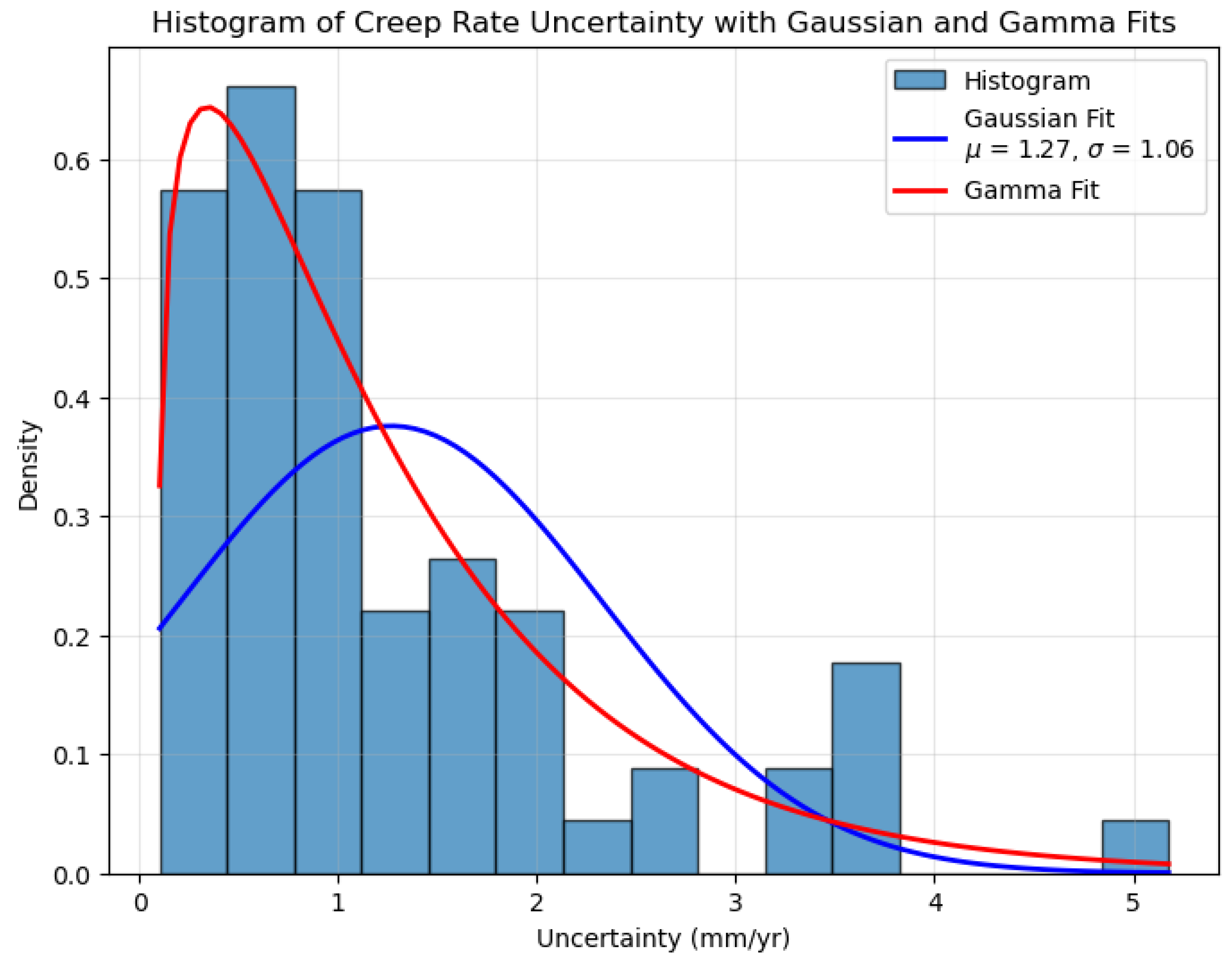
Creep rate uncertainty as suggested in [3] is 1.2 ± 1 (mm/year). The distribution of this uncertainty in measurement of the creep rate is shown in Figure 7. The data is loaded from a file (available in the GitHub repository for this project), assuming a two column structure separated by commas. First column is assumed to be the x(positions) and the second is the velocities . We also assume that the observational errors follow a Normal distribution, , where and , with respect to the model equation in Equation 3.
Figure 7.
Creep rate uncertainty distribution for the SAF based on high-resolution GPS and InSAR data from Ref. [3]. A Gaussian fit yields a mean of 1.27 mm/year, but heavy tails suggest a Gamma fit may be more appropriate, with a representative value of mm/year.
Figure 7.
Creep rate uncertainty distribution for the SAF based on high-resolution GPS and InSAR data from Ref. [3]. A Gaussian fit yields a mean of 1.27 mm/year, but heavy tails suggest a Gamma fit may be more appropriate, with a representative value of mm/year.
2.6. Two-Fault
The volocities are additive (superposition of two single-faults).
2.7. Defining Log-Likelihood and Log-Prior
We want to know how well the model fits the data.
When taking the Log-Likelihhood, the product becomes a sum. Given , it simplifies to
Where A is a constant throughout the MCMC process.
2.8. Bayesian Context
In Bayesian Context, the Posterior distribution of the parameters given the data , which is our goal, is given as:
is the likelihood (How probable the observed data is under specific parameter values). is our initial beliefs about the parameters. is the Evidence, which is a normalizing constant, which can be ignored in MCMC since we are sampling ratios. So in order to find the posterior, we need to compute the likelihood, which determines how well a given set of parameters explains the data y.
2.9. Log-Prior, Single Fault
We have a uniform prior, where is a constant if within bounds, and if not, zero. So log prior would be 0 if valid and if not. The purpose of this is to constrain parameter ranges. For instance, and D both range between 0 and 80 while ranges from -50 to 50.
2.10. Random Walk Metropolis Sampler : Markov Chain Monte Carlo (MCMC)
This algorithm implements the Metropolis-Hastings MCMC algorithm. Starting at an initial guess, we propose a new point with S being the step scale. We then compute the log-posterior by taking the log of eq. 7, we arrive at:
The outputs are chain of samples, log-posterior values and acceptance rate.
2.11. Applying MCMC: Single Fault Model Analysis
The mean and STD of , D, are our posterior stats. The posterior distribution and correlations are plotted in Figure 8.
The MCMC model run over 30,000 samples burn-in of 5,000, step size 1.0:
2.12. Posterior Samples VS Data
Plot of the posterior samples vs Data is shown in Figure 11.
2.13. RMSE and the Two-Fault Model
The RMSE is defined as
where are the observations of the velocity, are the standard deviations of the model errors and is the velocity at location , using parameters . The RMSE for single-fault model is approximately . This is not disastrous, but not ideal either. To improve this, we consider a modified version of this model, namely "Two-Fault" model and see if we can arrive at a better RMSE.
Single Fault Model Parameters are displayed in Table 1.
2.14. The Two-Fault Model
In this model, instead of one fault, we consider two faults. We start by two-fault velocity, generalizing equation 3. , arriving at
The MCMC analysis is similar to that of single-fault model. The Two Fault Model Parameters are calculated and shown in Table 2.
Figure 9.
Triangle corner plot of two-fault model Parameters, obtained using the two-fault velocity model. The velocities are in (mm/year), Depth and x are in (km).
Figure 9.
Triangle corner plot of two-fault model Parameters, obtained using the two-fault velocity model. The velocities are in (mm/year), Depth and x are in (km).
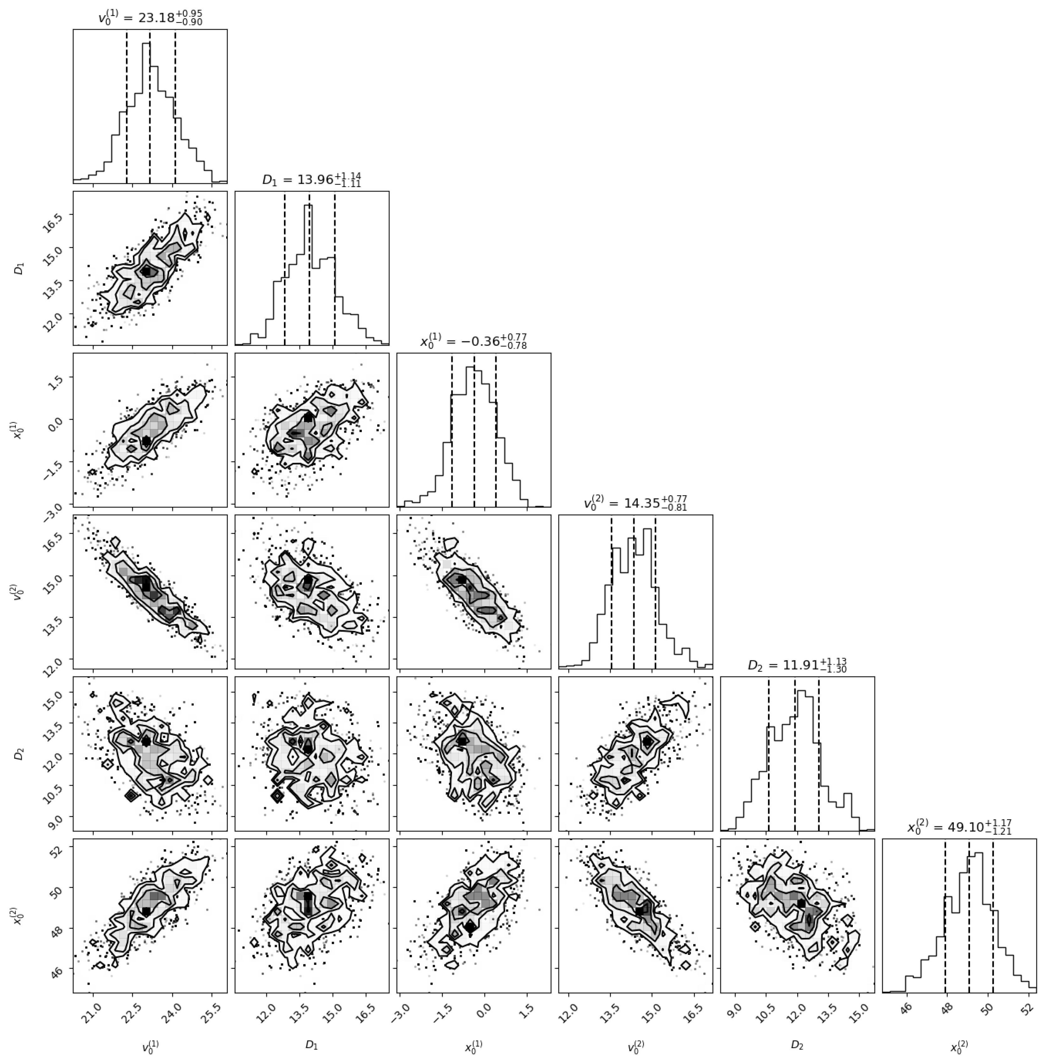
It is noteworthy that there is a negative correlation between the two velocities and and these are exclusively shown in Figure 10.
For model validation, posterior samples are directly compared to experimental data. The error bars are not graphically displayed since they are relatively small and the points in Figure 11 overlap in representing the data and the corresponding uncertainty.
Figure 11.
Posterior Samples VS Experimental Data for the geophysical single-fault model. The model fits well, but it is not ideal, given a relatively large RMSE of 1.4.
Figure 11.
Posterior Samples VS Experimental Data for the geophysical single-fault model. The model fits well, but it is not ideal, given a relatively large RMSE of 1.4.
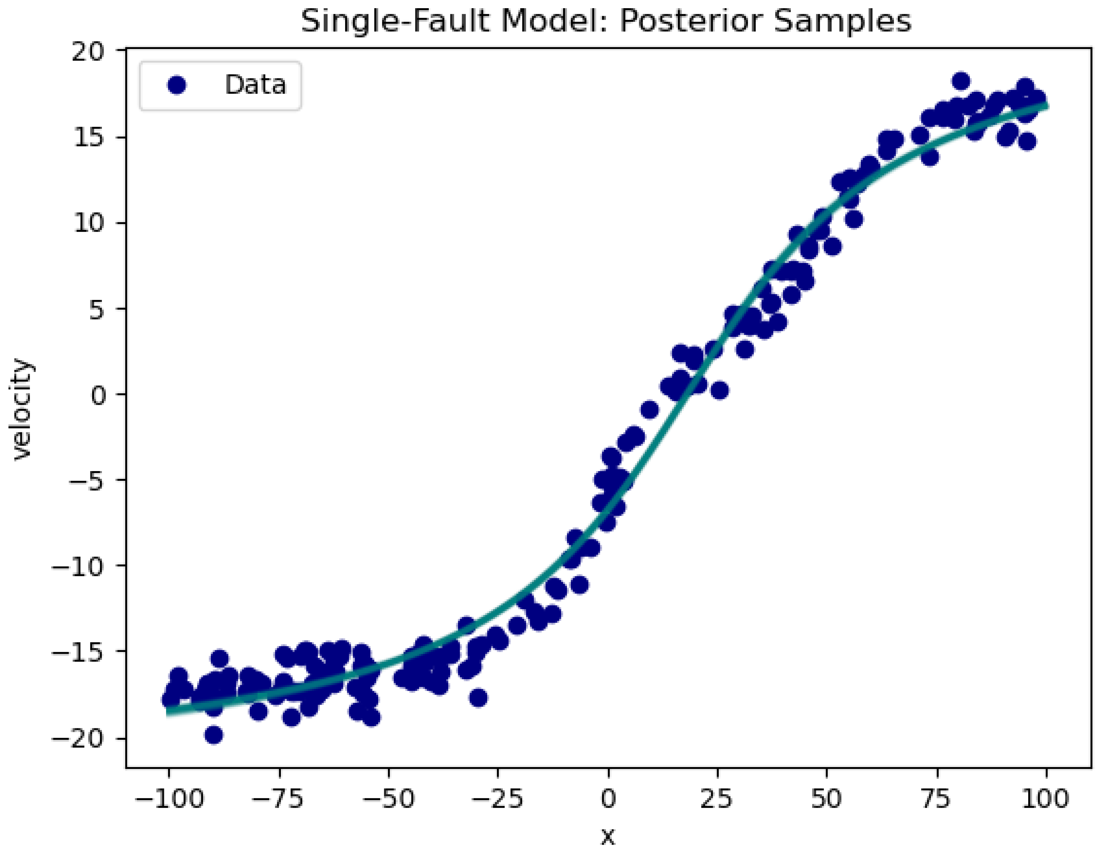
Although not very far from 1, the value of 1.4 for the RMSE is not ideal. Particularly around the origin (see Figure 11), the deviation of data from model become more obvious.
Figure 12.
Two Fault Model Posterior VS Experimental Data. The RMSE is ≈ 1. The model fits data within expected uncertainty.
Figure 12.
Two Fault Model Posterior VS Experimental Data. The RMSE is ≈ 1. The model fits data within expected uncertainty.
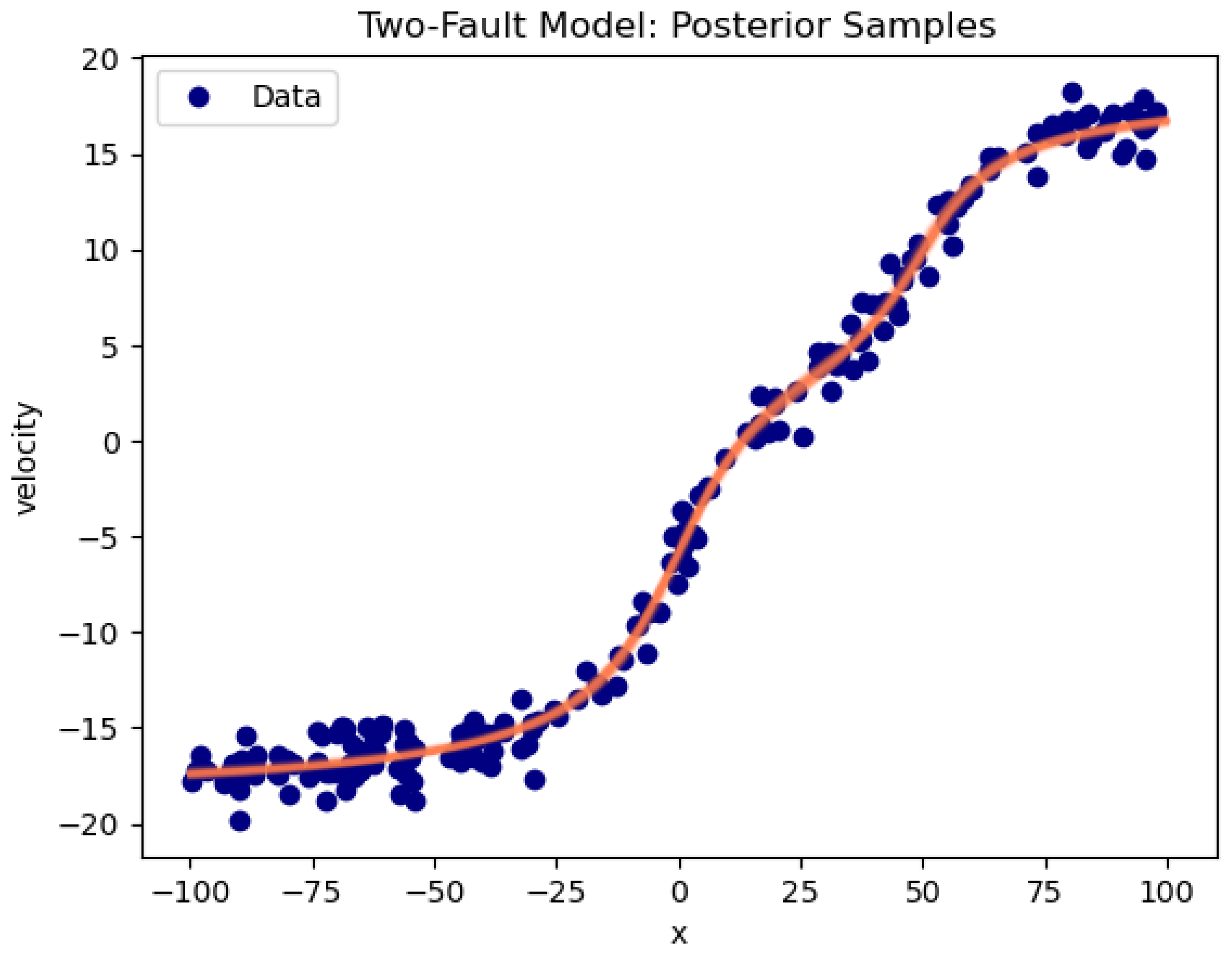
Figure 13.
Two-Fault Model RMSE distribution, which is centered around value of 1. This is expected, given the background noise of around 1 mm/year.
Figure 13.
Two-Fault Model RMSE distribution, which is centered around value of 1. This is expected, given the background noise of around 1 mm/year.
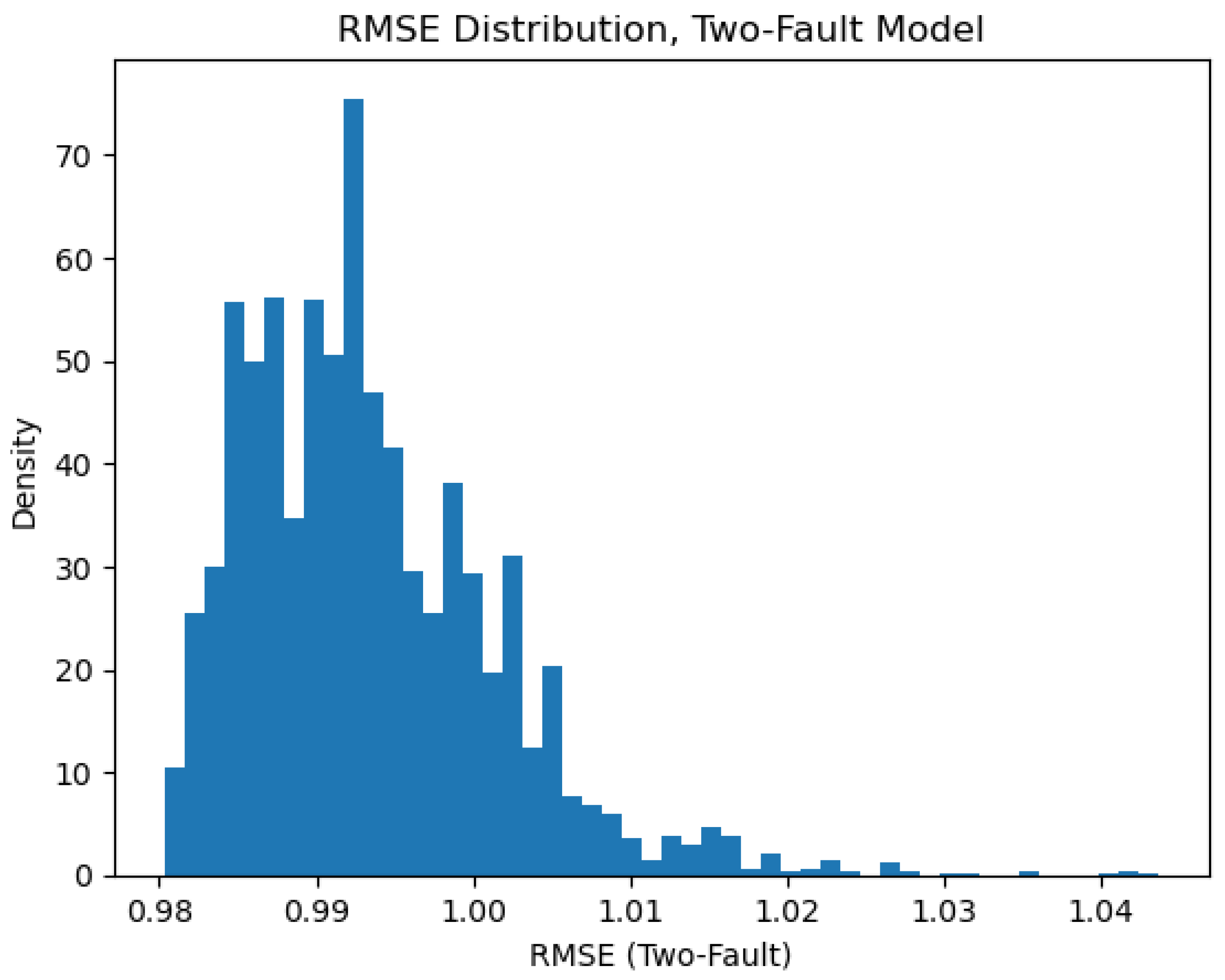
Heavy tails in the RMSE usually hint at unexpected noise, systemic error or even model inadequacy.
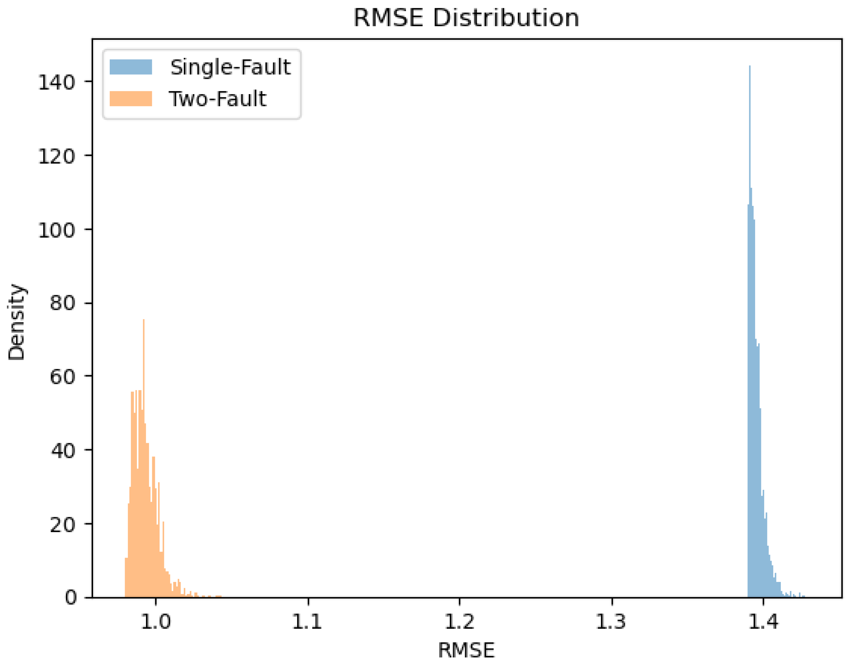
Figure 14.
Two Fault Model RMSE distribution ≈ 1 (Left) VS Single Fault RMSE ≈ 1.4 (Right). This RMSE compares closely to the background noise level, further strengthening the two-fault hypothesis.
Figure 14.
Two Fault Model RMSE distribution ≈ 1 (Left) VS Single Fault RMSE ≈ 1.4 (Right). This RMSE compares closely to the background noise level, further strengthening the two-fault hypothesis.
2.15. Fault Analysis: Discussion
Markov Chain Monte Carlo is a powerful method for Data Analysis. In this study, it was used as a tool in Inverse Problem, fitting model parameters to data. This geophysical model elegantly fit to data of 200 points. Using a single-fault model, the parameters were obtained, however with a RMSE of 1.4, which was not ideal. Therefore a Two-fault model was examined, arriving at a RMSE of 1. Given the expected variance as seen in figure (7), this RMSE is in a good agreement with the data. The ration of this RMSE to the STD is given in eq. 11.
These parameters and their error bars are plotted and presented in Figure 15.
The RMSE is already improved to the level of background noise and this can be easily seen comparing Figure 7 and Figure 14.
Having achieved a reasonable RMSE, one can further explore ways to reduce RMSE, given a predictive model. One can use Kalman Gain to smooth such data:
Here, is the Kalman Gain itself, is the prior estimate cov. matrix of the current state, H is the observation matrix and is the measurement noise cov. matrix. The non-linear Kalman Filter (Unscented Kalman Filter)is used for systems with non-linearity.
This method, applied to the two-fault model, reduces the RMSE even further (RMSE ≈ 0.9). A comparison is shown in Figure 16.
and all RMSE distributions have been plotted in Figure 17.
This suggests that the SAF does not act in isolation and is influenced by other fault systems such as San Jacinto fault (SJF) in southern California, which can contribute to the velocity field. The (14 ± 1) is consistent with the the SJF velocity rate of (11 ± 4) mm/yr reported by Rockwell et al. [30].
3. Anthropogenic Seismicity
Under load, soil deforms gradually at a variable rate, a phenomenon known as consolidation, mathematically formulated by Biot in 1940 [31]. Hill et. al.[32] argue that stress perturbations in the order of 0.5 MPa are sufficient to trigger seismicity. These perturbations are dominated by pore pressure changes. They furthermore correlated the past 6 major earthquake events on the SAF with high-stands of the ancient Lake Cahuilla, which its remnant is known today as the Salton Sea (shown in Figure 18). Using Finite Element Methods (FEM) to arrive at such correlations, their model seems to be applicable to other regions where hydrologic loading is associated with seismicity, anthropogenic or not.
3.1. Seismic Risk Threshold
Higher pressures of fluid introductions are usually carried out over shorter periods of time and lower pressures are carried out over a larger period of time. In other words, there is a tradeoff. When examined as a complex system, this resembles a path which constraints the system’s evolution in which soil consolidation undergoes dissipation.
A breakdown of these operations and their corresponding share of caused anthropogenic seismicity can be found in Figure 19.
3.2. Oil and Gas Operations
3.3. CCS & Wastewater
CO2 injection stimulates plate tectonics due to mechanical pressure exerted by the injected fluids. In the past few years, as part of broader mitigation efforts, has been injected into the earth. It is postulated that the injected stays underground for decades. The pressure excreted by this gas can however threaten the integrity of the seals at injection sites. This requires further analysis on the operations as well as more simulations which could shed light on anthropogenic seismicity caused by geological injections. Zoback et. al. argue that in order to reduce the risk of seismicity from such operations, the (pressure), as shown in my uncertainty relationship (??), should be limited. Increasing pressure can also trigger an earthquake and as a result, threaten the integrity of the CCS seals. A map of areas in the United States with active or potential CCS operations is shown in Figure 20.
3.4. Geothermal: The Brawley seismic zone (BSZ)
The Brawley seismic zone encompasses Salton Sea and the surronding area and is home to Geothermal operations, most notably the Imperial Valley Geothermal Project. It has a MW of geothermal capacity. It also provides a high level of battery-grade lithium for electric vehicles (currently at ∼ 75,000 tons) [39]. Despite the strategic advantages, it has also introduced background level seismicity to the region, particularly at the North Brawley Geothermal Field (NBGF) and at the Salton Sea Geothermal Field (SSGF) [40]. .
3.5. Policy Error: The 1906 San Francisco Earthquake
In 1905, the Colorado River flooded the Salton Sink due to a failed irrigation project, forming the Salton Sea. In 1906, San Francisco experienced a magnitude 7.9 earthquake, leaving over 3,000 casualties. Supported by paleo-seismic data, major SAF earthquakes are shown to be modulated by ancient lake-fillings [32].
4. Sea Level Rise
Sea level rise (SLR), estimated at mm/year globally [41], increases water loads, inducing pressure changes that can trigger seismicity. Figure 21 illustrates the correlation between rising CO2 levels, sea level, and temperature anomalies from 1959 to 2020, highlighting the SLR [42,43,44].
The mechanism can be explained by the pore pressure in a poroelastic medium, induced by hydrologic loads from sea level rise, satisfies the following diffusion equation derived from Biot’s theory of poroelasticity, which is a diffusion PDE:
This equation basically shows the relationship between pressure change as well as temporal and spatial diffusion. p is the fluid pressure, M is the Biot modulus, is the Hydraulic conductivity, with k being permeability and the fluid viscosity. is the Biot-Willis coefficient, is the Volumetric strain where u is the solid displacement vector. is the Laplacian operator.
4.1. Relation to Seismicity
The pore pressure p alters the effective stress on faults, following Terzaghi’s principle:
where is the effective normal stress. An increase in p reduces , which may trigger fault failure under the Coulomb failure criterion:
where is Critical shear stress, is Friction coefficient.
For SLR, the slow loading rate () induces small over large , resembling low-pressure, long-timescale processes (e.g., CO2 injection in CCS). The product indicates that cumulative pore pressure changes can still meet or exceed , potentially triggering seismicity in critically stressed fault systems.
4.2. Seismicity Triggering
The pore pressure p from Equation (13) reduces the effective normal stress on faults, following Terzaghi’s principle:
where is the effective stress. A decrease in brings faults closer to failure under the Coulomb criterion:
where is the critical shear stress, is the friction coefficient, and C is cohesion.
5. Online Forecasting Models
Broccardo et al. [46] developed a Bayesian model based on a nonhomogeneous Poisson process (NHPP) to forecast induced seismicity. A successful decision-making criterion emerging from such model, would benefit the communities. Such forecasting models can also be used in other areas of anthropogenic activities known to cause seismicity.
The probability of observing seismic events in the time window , given the observed data up to time (t), , or simply , is:
represents the predictive probability of observing seismic events in a future time window , given observed data . Here, is the number of events in the time window of interest, is the time dependent seismicity rate which depends on model parameters and is the expectation value of the number of events in that interval. The first term is the Poisson probability of observing events, given the rate.
The posterior distribution updates the knowledge about , using , and the integral over takes into account the uncertainties by averaging.
6. Discussions & Policy Recommendations
Bayesian Inference certainly helps us better understand anthropogenic risks. Modern analysis tools such as the MCMC are therefore certainly useful in shedding light on contemporary problems in Earth Science and particularly inverse problems in geophysics.
Bayesian inference cannot compensate for missing data or poorly designed experiments. No data analysis tool can generate information absent from the data. That said, Bayesian inference could be used to better arrange for experimental setups to hunt for information that otherwise could not be captured [47]. This approach can even further improve geophysics experiments which could contribute to the understanding of Earth and planetary processes and anthropogenic risk factors in seismicity. Given the complexity of the issue of induced seismicity, effective data assimilation and analysis as well as up to date analysis tools and technologies are required to minimize the impact of activities which would cause anthropogenic seismicity. Several guidelines, such as the ETH Zürich “Good-Practice Guide for Managing Induced Seismicity in Deep Geothermal Energy Projects in Switzerland” [48], exist. These should be updated to incorporate new physics-informed methods discussed herein.
Acknowledgments
The author is thankful to Corey J. Gabriel and Matthew Weingarten for fruitful discussions.
References
- Turcotte, D.L.; Malamud, B.D. Earthquakes as a complex system. In International Geophysics; Elsevier, 2002; Vol. 81, pp. 209–cp1.
- Sieh, K.; Stuiver, M.; Brillinger, D. A more precise chronology of earthquakes produced by the San Andreas fault in southern California. Journal of Geophysical Research: Solid Earth 1989, 94, 603–623. [Google Scholar] [CrossRef]
- Tong, X.; Sandwell, D.; Smith-Konter, B. High-resolution interseismic velocity data along the San Andreas Fault from GPS and InSAR. Journal of Geophysical Research: Solid Earth 2013, 118, 369–389. [Google Scholar] [CrossRef]
- Carpenter, B.; Marone, C.; Saffer, D. Weakness of the San Andreas Fault revealed by samples from the active fault zone. Nature Geoscience 2011, 4, 251–254. [Google Scholar] [CrossRef]
- Collettini, C.; Niemeijer, A.; Viti, C.; Marone, C. Fault zone fabric and fault weakness. Nature 2009, 462, 907–910. [Google Scholar] [CrossRef]
- Moore, D.E.; Rymer, M.J. Talc-bearing serpentinite and the creeping section of the San Andreas Fault. Nature 2007, 448, 795–797. [Google Scholar] [CrossRef] [PubMed]
- Scholz, C.H. Evidence for a strong San Andreas Fault. Geology 2000, 28, 163–166. [Google Scholar] [CrossRef]
- Vilarrasa, V.; Carrera, J.; Olivella, S.; Rutqvist, J.; Laloui, L. Induced seismicity in geologic carbon storage. Solid Earth 2019, 10, 871–892. [Google Scholar] [CrossRef]
- Walker, J.C.; Hays, P.; Kasting, J.F. A negative feedback mechanism for the long-term stabilization of Earth’s surface temperature. Journal of Geophysical Research: Oceans 1981, 86, 9776–9782. [Google Scholar] [CrossRef]
- Penman, D.E.; Caves Rugenstein, J.K.; Ibarra, D.E.; Winnick, M.J. Silicate weathering as a feedback and forcing in Earth’s climate and carbon cycle. Earth-Science Reviews 2020, 209, 103298. [Google Scholar] [CrossRef]
- Archer, D. Fate of fossil fuel CO2 in geologic time. Journal of geophysical research: Oceans 2005, 110. [Google Scholar] [CrossRef]
- Archer, D.; Eby, M.; Brovkin, V.; Ridgwell, A.; Cao, L.; Mikolajewicz, U.; Caldeira, K.; Matsumoto, K.; Munhoven, G.; Montenegro, A.; et al. Atmospheric lifetime of fossil fuel carbon dioxide. Annual review of earth and planetary sciences 2009, 37, 117–134. [Google Scholar] [CrossRef]
- Colbourn, G.; Ridgwell, A.; Lenton, T. The time scale of the silicate weathering negative feedback on atmospheric CO2. Global Biogeochemical Cycles 2015, 29, 583–596. [Google Scholar] [CrossRef]
- Meissner, K.J.; McNeil, B.I.; Eby, M.; Wiebe, E.C. The importance of the terrestrial weathering feedback for multimillennial coral reef habitat recovery. Global Biogeochemical Cycles 2012, 26. [Google Scholar] [CrossRef]
- Batalha, N.E.; Kopparapu, R.K.; Haqq-Misra, J.; Kasting, J.F. Climate cycling on early Mars caused by the carbonate–silicate cycle. Earth and Planetary Science Letters 2016, 455, 7–13. [Google Scholar] [CrossRef]
- Laine, M. Adaptive MCMC methods with applications in environmental and geophysical models; Finnish Meteorological Institute, 2008.
- Malinverno, A. Parsimonious Bayesian Markov chain Monte Carlo inversion in a nonlinear geophysical problem. Geophysical Journal International 2002, 151, 675–688. [Google Scholar] [CrossRef]
- Menke, W. Geophysical data analysis: Discrete inverse theory; Academic Press, 2018.
- Sambridge, M.; Mosegaard, K. Monte Carlo methods in geophysical inverse problems. Reviews of Geophysics 2002, 40, 3–1. [Google Scholar] [CrossRef]
- Trotta, R. Bayes in the sky: Bayesian inference and model selection in cosmology. Contemporary Physics 2008, 49, 71–104. [Google Scholar] [CrossRef]
- Rahemi, R. Variation in electron work function with temperature and its effect on the Young’s modulus of metals. Scripta materialia 2015, 99, 41–44. [Google Scholar] [CrossRef]
- Chang, J.; Nikolaev, P.; Carpena-Núñez, J.; Rao, R.; Decker, K.; Islam, A.E.; Kim, J.; Pitt, M.A.; Myung, J.I.; Maruyama, B. Efficient closed-loop maximization of carbon nanotube growth rate using Bayesian optimization. Scientific reports 2020, 10, 9040. [Google Scholar] [CrossRef]
- Uncertainty quantification of pollutant source retrieval: comparison of Bayesian methods with application to the Chernobyl and Fukushima Daiichi accidental releases of radionuclides 2017. 143, 2886–2901.
- Sakuragi, Y.; Meason, J.L.; Kuroda, P.K. Uranium and plutonium isotopes in the atmosphere. Journal of Geophysical Research 1983, 88, 3718–3724. [Google Scholar] [CrossRef]
- Menke, W. Geophysical data analysis: Discrete inverse theory; Academic Press, 2018.
- Li, A. Topics In Data Science: Data Analysis In Physics Lectures; Halıcıoğlu Data Science Institute: La Jolla, California, 2025. [Google Scholar]
- Savage, J.C.; Burford, R.O. Geodetic determination of relative plate motion in central California. Journal of Geophysical Research 1973, 78, 832–845. [Google Scholar] [CrossRef]
- IGPP. Instituge Of Geophysics and Planatary Physics; 2024.
- MORZFELD, M. Geophysical Data Analysis SIOG223- Class Notes; 2024.
- Rockwell, T.K.; Dawson, T.E.; Young Ben-Horin, J.; Seitz, G. A 21-event, 4,000-year history of surface ruptures in the Anza seismic gap, San Jacinto Fault, and implications for long-term earthquake production on a major plate boundary fault. Pure and Applied Geophysics 2015, 172, 1143–1165. [Google Scholar] [CrossRef]
- Biot, M.A. General theory of three-dimensional consolidation. Journal of applied physics 1941, 12, 155–164. [Google Scholar] [CrossRef]
- Hill, R.G.; Weingarten, M.; Rockwell, T.K.; Fialko, Y. Major southern San Andreas earthquakes modulated by lake-filling events. Nature 2023, 618, 761–766. [Google Scholar] [CrossRef] [PubMed]
- Human-Induced Earthquake Database (HiQuake). Induced Earthquakes, 2025. Accessed: 2025-04-27.
- Talwani, P. On the nature of reservoir-induced seismicity. Pure and applied Geophysics 1997, 150, 473–492. [Google Scholar] [CrossRef]
- Deng, F.; Dixon, T.H.; Xie, S. Surface deformation and induced seismicity due to fluid injection and oil and gas extraction in western Texas. Journal of Geophysical Research: Solid Earth 2020, 125, e2019JB018962. [Google Scholar] [CrossRef]
- Argus, D.F.; Heflin, M.B.; Peltzer, G.; Crampé, F.; Webb, F.H. Interseismic strain accumulation and anthropogenic motion in metropolitan Los Angeles. Journal of Geophysical Research: Solid Earth 2005, 110. [Google Scholar] [CrossRef]
- Office of the Governor of California. California Moves to Prevent New Oil Drilling Near Communities, Expand Health Protections, 2021. Accessed: 2025-05-12.
- of the Interior, U.D. National Assessment of Geologic Carbon Dioxide Storage Resources-Data. Technical report, 2013.
- Los Angeles Times. Lithium will fuel the clean energy boom. This company may have a breakthrough. Los Angeles Times.
- Llenos, A.L.; Michael, A.J. Characterizing potentially induced earthquake rate changes in the Brawley seismic zone, southern California. Bulletin of the Seismological Society of America 2016, 106, 2045–2062. [Google Scholar] [CrossRef]
- Melini, D.; Piersanti, A. Impact of global seismicity on sea level change assessment. Journal of Geophysical Research: Solid Earth 2006, 111. [Google Scholar] [CrossRef]
- Keeling, C.D.; Piper, S.C.; Bacastow, R.B.; Wahlen, M.; Whorf, T.P.; Heimann, M.; Meijer, H.A. Exchanges of atmospheric CO2 and 13CO2 with the terrestrial biosphere and oceans from 1978 to 2000. I. Global aspects. SIO Reference Series 01-06, Scripps Institution of Oceanography, San Diego, 2001.
- Church, J.A.; White, N.J.; Konikow, L.F.; Domingues, C.M.; Cogley, J.G.; Rignot, E.; Gregory, J.M.; van den Broeke, M.R.; Monaghan, A.J.; Velicogna, I. Revisiting the Earth’s sea-level and energy budgets from 1961 to 2008. Geophysical Research Letters 2011, 38. [Google Scholar] [CrossRef]
- Met Office Hadley Centre and Climatic Research Unit. HadCRUT5: Global historical surface temperature anomalies dataset, 2025. Version HadCRUT.5.0.2.0, Accessed: 2025-04-27.
- University of Hawaii Sea Level Center. UHSLC – University of Hawaii Sea Level Center, 2025. Accessed: 2025-04-27.
- Broccardo, M.; Mignan, A.; Wiemer, S.; Stojadinovic, B.; Giardini, D. Hierarchical Bayesian modeling of fluid-induced seismicity. Geophysical Research Letters 2017, 44, 11–357. [Google Scholar] [CrossRef]
- Von Toussaint, U. Bayesian inference in physics. Reviews of Modern Physics 2011, 83, 943–999. [Google Scholar] [CrossRef]
- Kraft, T.; Roth, P.; Ritz, V.; Antunes, V.; Toledo Zambrano, T.A.; Wiemer, S. Good-Practice Guide for Managing Induced Seismicity in Deep Geothermal Energy Projects in Switzerland. Technical report, ETH Zurich, 2025.
| 1 | Prior Knowledge, or simply the prior: Initial probability distribution assigned to a parameter or hypothesis before observing new data |
Figure 1.
Creep rate data heatmap across the SAF, extending roughly 750 miles between (, ) and (, ). InSAR and GPS dataset from Ref. [3]. The creep rate peaks between and , with a maximum of mm/year at (, ).
Figure 1.
Creep rate data heatmap across the SAF, extending roughly 750 miles between (, ) and (, ). InSAR and GPS dataset from Ref. [3]. The creep rate peaks between and , with a maximum of mm/year at (, ).
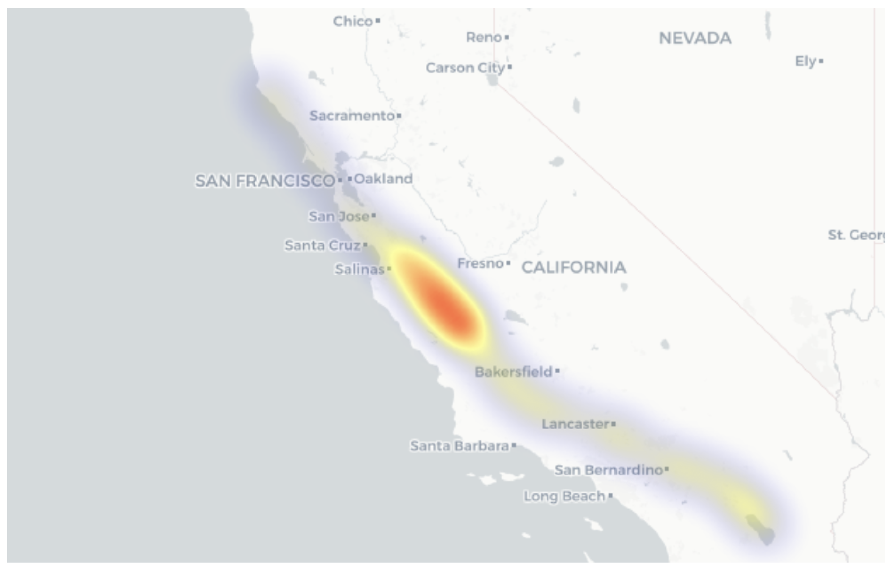
Figure 2.
PDF (Probability Density Function) and CDF (Cumulative Density Function) for large earthquake events associated with the SAF, using the datasets from Ref. [2]. The reduction in probability is explained using the theory that the fault-zone material do not heal after each de-formation and they lack strength needed to cause more destructive movements [4].
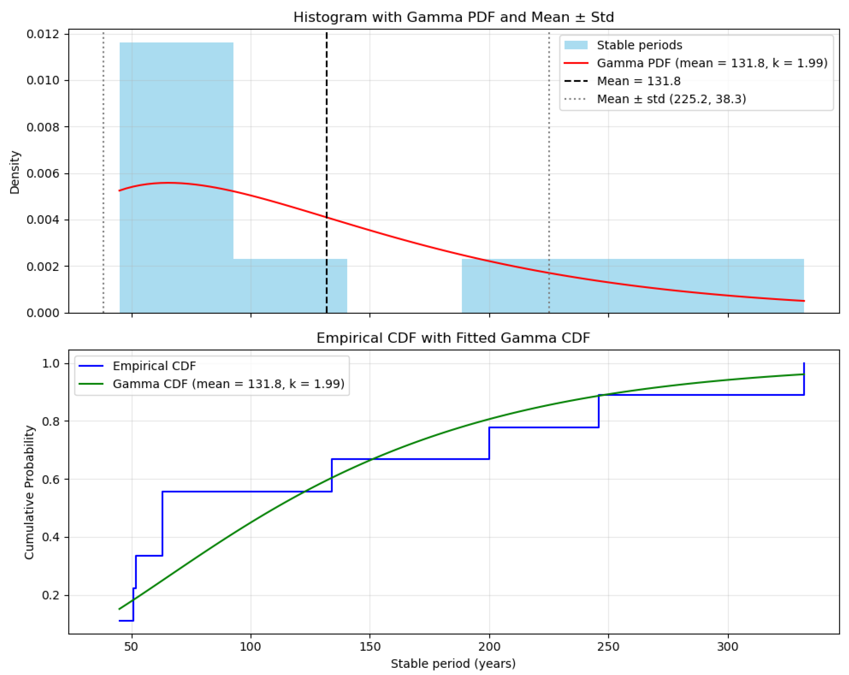
Figure 3.
Geomagnetic reversal timeline. The last reversal happened around 0.78 MYrs ago, with the probability of reversals decreasing with time.
Figure 3.
Geomagnetic reversal timeline. The last reversal happened around 0.78 MYrs ago, with the probability of reversals decreasing with time.
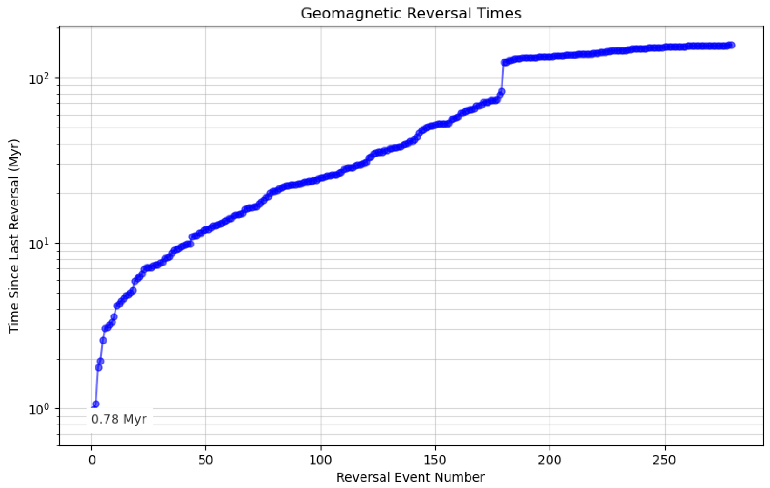
Figure 4.
Creep rate versus location visualized in a Cartopy projection. Raw datasets from Ref. [3]. The creep rate peaks between and , with a maximum of mm/year at (, ).
Figure 4.
Creep rate versus location visualized in a Cartopy projection. Raw datasets from Ref. [3]. The creep rate peaks between and , with a maximum of mm/year at (, ).
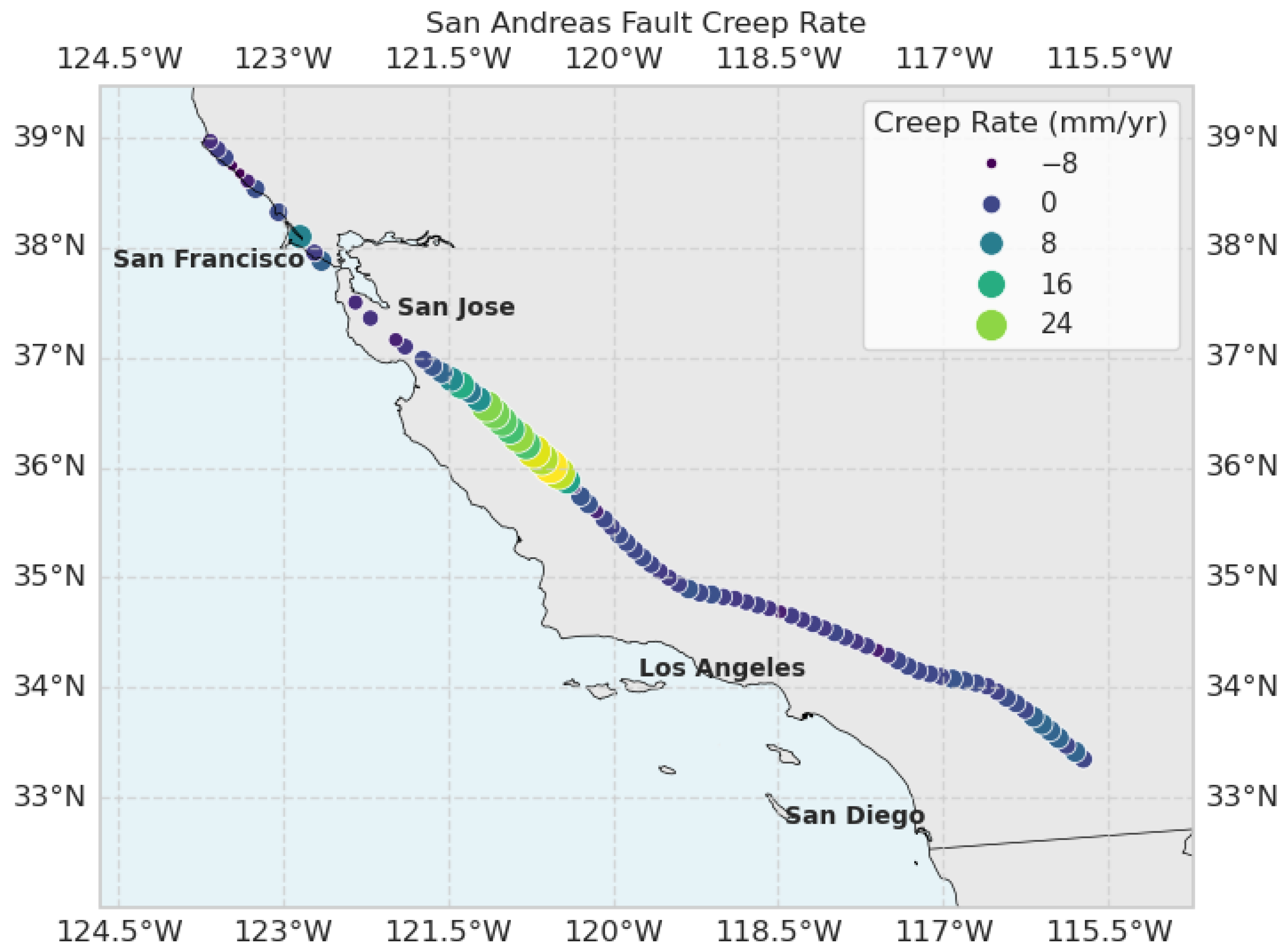
Figure 5.
Creep rate vs Latitude and the corresponding uncertainties. Distributions of the uncertainties are plotted and shown in Figure 7. Higher latitudes show a greater rate of uncertainty in creep rate.
Figure 5.
Creep rate vs Latitude and the corresponding uncertainties. Distributions of the uncertainties are plotted and shown in Figure 7. Higher latitudes show a greater rate of uncertainty in creep rate.
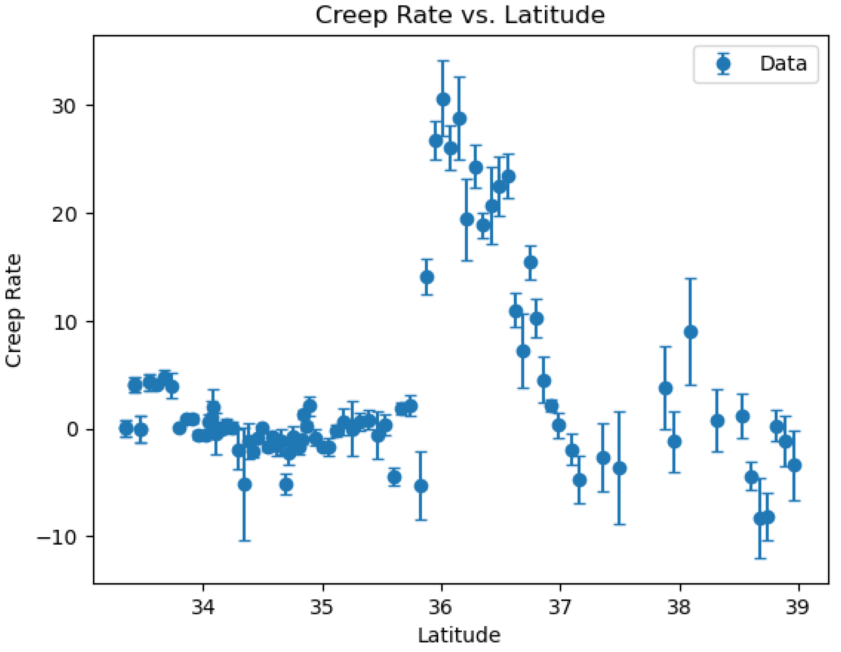
Figure 6.
Creep rate model with Gaussian process regression targeting creep rate and its uncertainties. Higher creep rate uncertainties result in greater model uncertainty. Experimental improvements could enhance the predictive model.
Figure 6.
Creep rate model with Gaussian process regression targeting creep rate and its uncertainties. Higher creep rate uncertainties result in greater model uncertainty. Experimental improvements could enhance the predictive model.
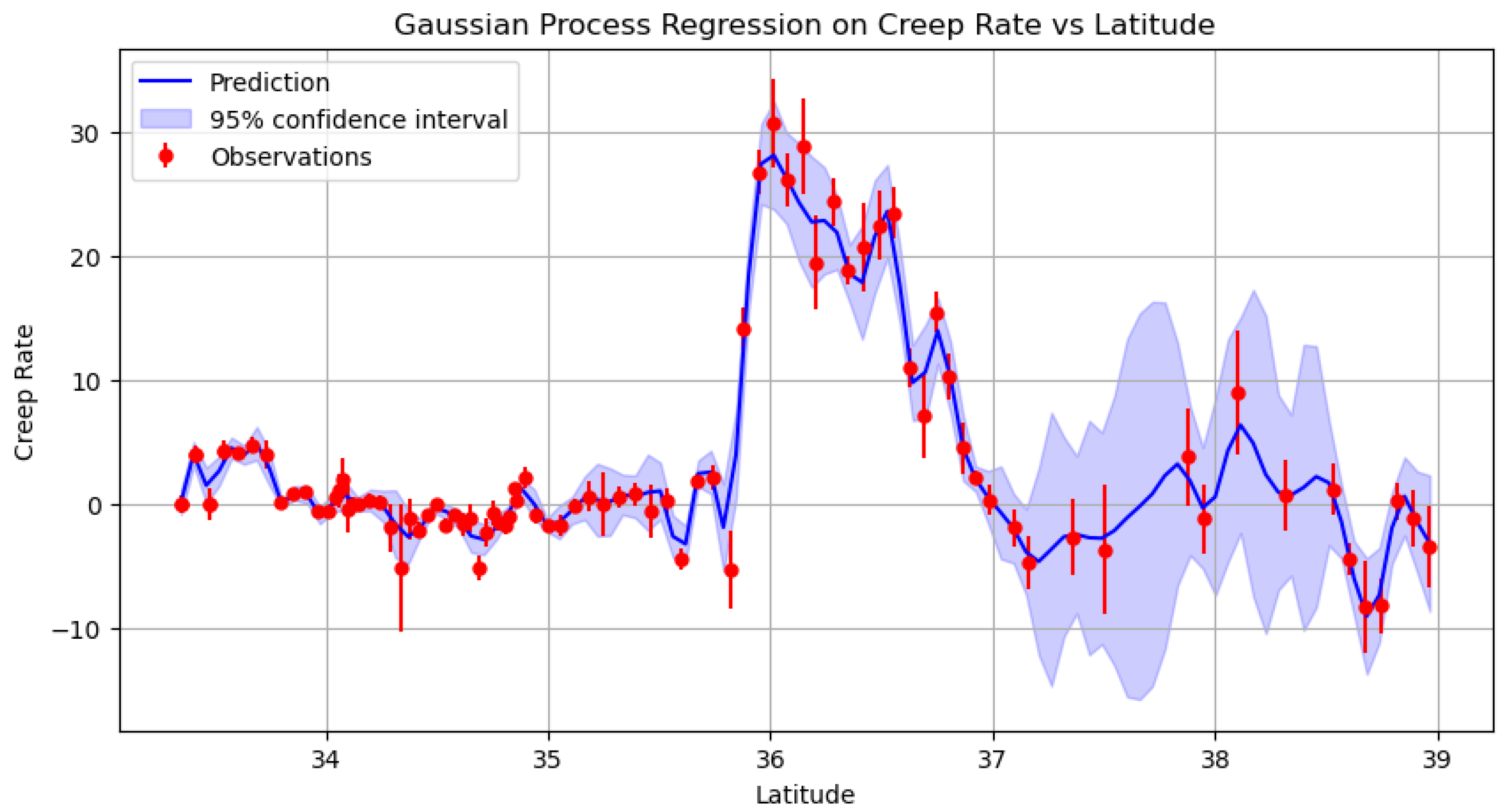
Figure 8.
Posterior distribution and correlations for the single-fault model. The plot includes data and 100 random posterior model curves. Single-fault acceptance rate: 11%. Posterior means: [45.53, 36.05, 18.34]; standard deviations: [0.61, 1.13, 0.35]. Velocities are in mm/year; depth and x are in km.
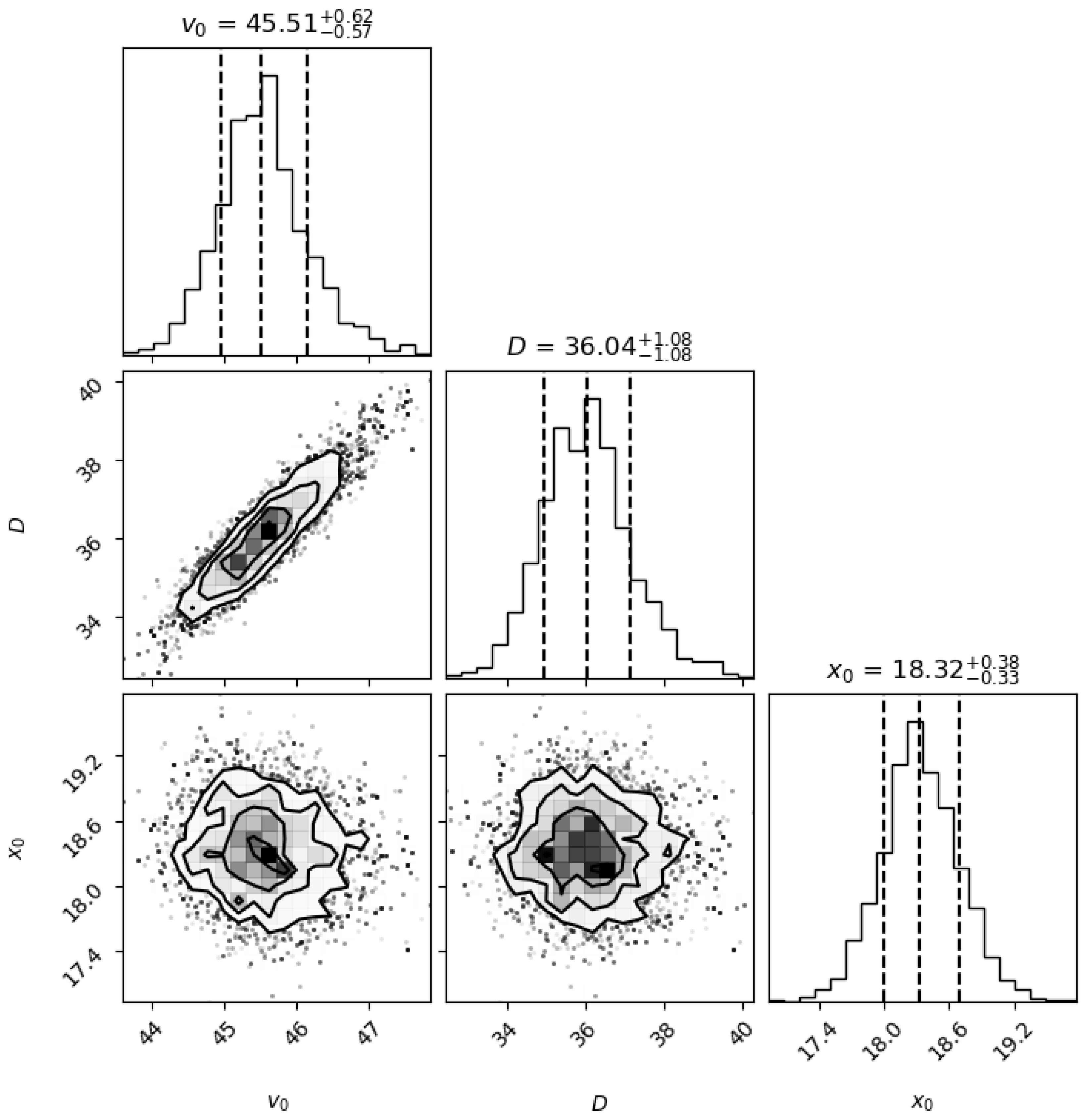
Figure 10.
The negative correlation between the two velocities and are shown here. This suggests that the velocity directions are opposite.
Figure 10.
The negative correlation between the two velocities and are shown here. This suggests that the velocity directions are opposite.
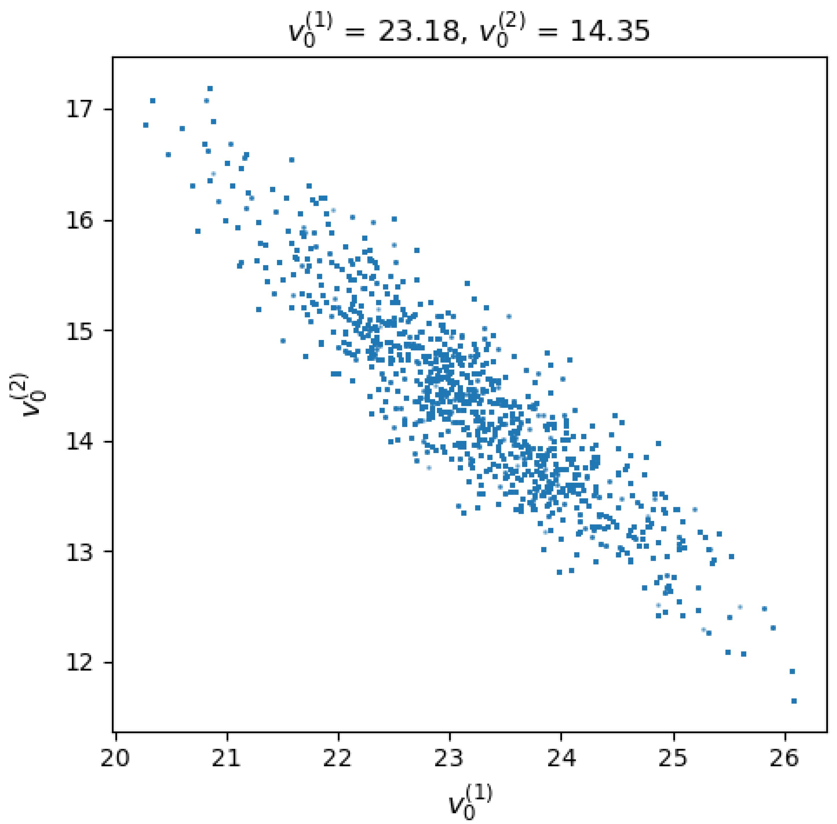
Figure 15.
Model Parameter Values and their corresponding uncertainties, within 95 % Confidence Interval. The two-fault model is more appropriate, given the likelihood of San Jacinto Fault as a candidate for the influencing system.
Figure 15.
Model Parameter Values and their corresponding uncertainties, within 95 % Confidence Interval. The two-fault model is more appropriate, given the likelihood of San Jacinto Fault as a candidate for the influencing system.
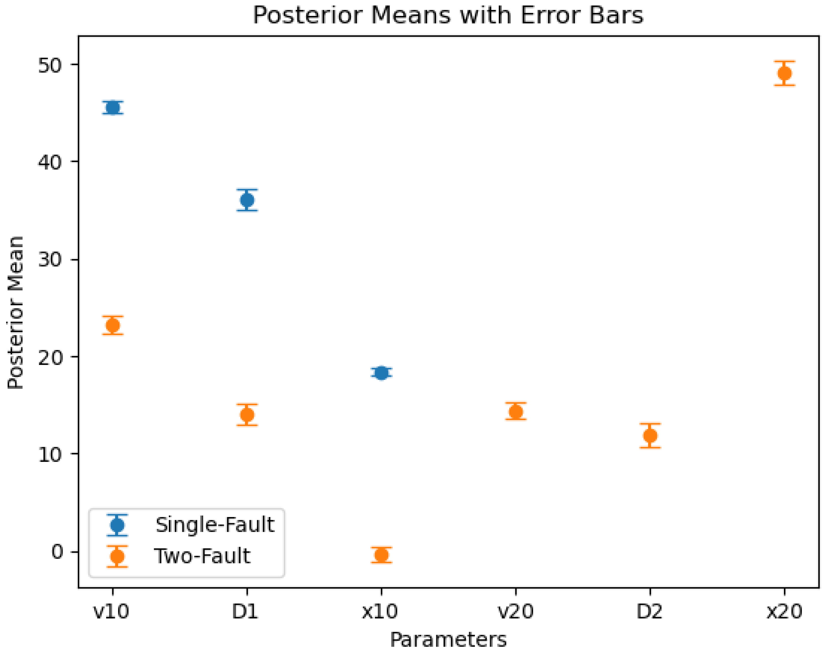
Figure 16.
Noise reduction using Unscented Kalman Filter assuming a non-linear mechanism. The RMSE was further reduced.
Figure 16.
Noise reduction using Unscented Kalman Filter assuming a non-linear mechanism. The RMSE was further reduced.
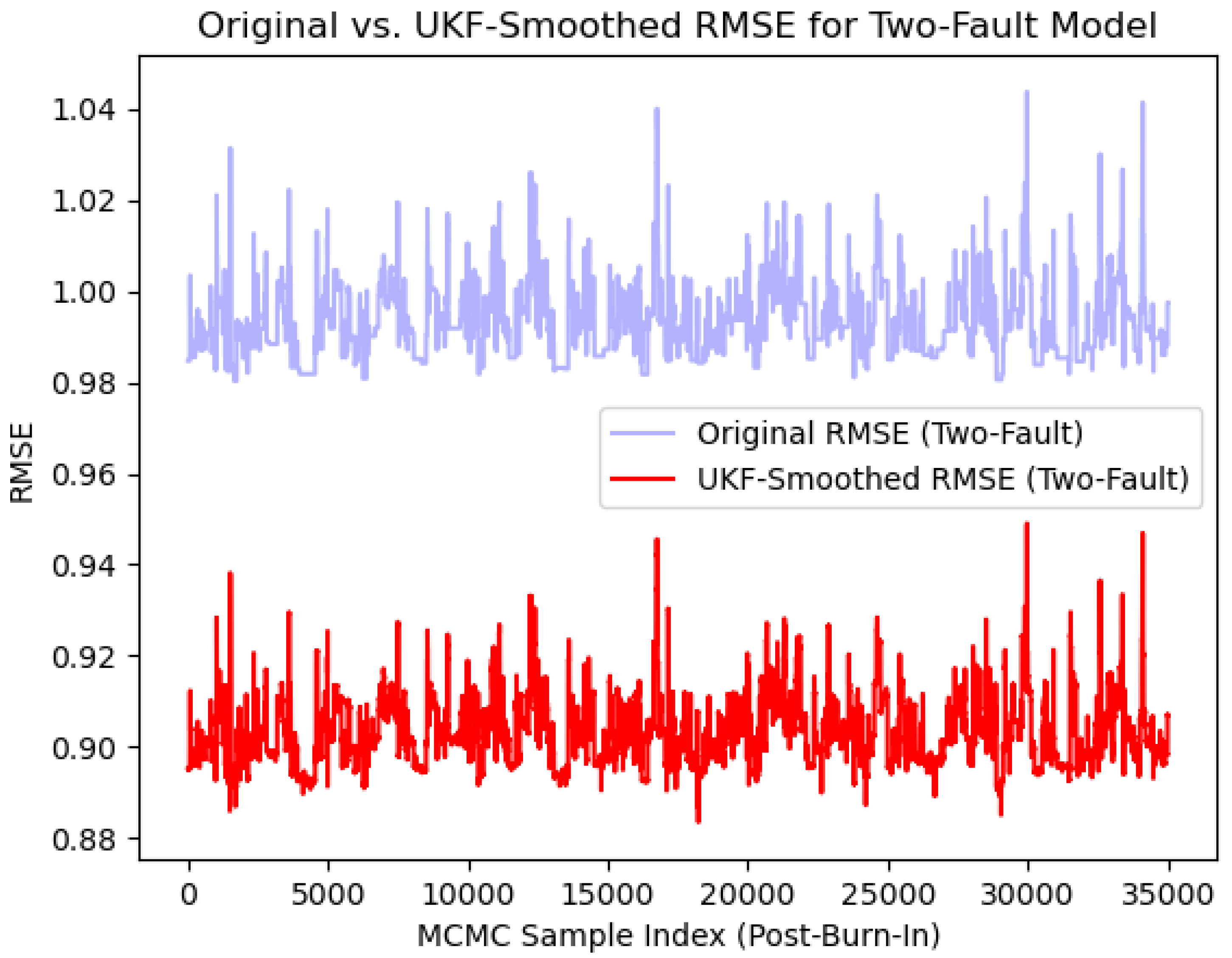
Figure 17.
The RMSE ≈ 1.4 for a single fault model was reduced to RMSE ≈ 1 using a two-fault model and was further reduced using an unscented Kalman filter to RMSE ≈ 0.9. Reducing the RMSE further might result in over-fitting.
Figure 17.
The RMSE ≈ 1.4 for a single fault model was reduced to RMSE ≈ 1 using a two-fault model and was further reduced using an unscented Kalman filter to RMSE ≈ 0.9. Reducing the RMSE further might result in over-fitting.
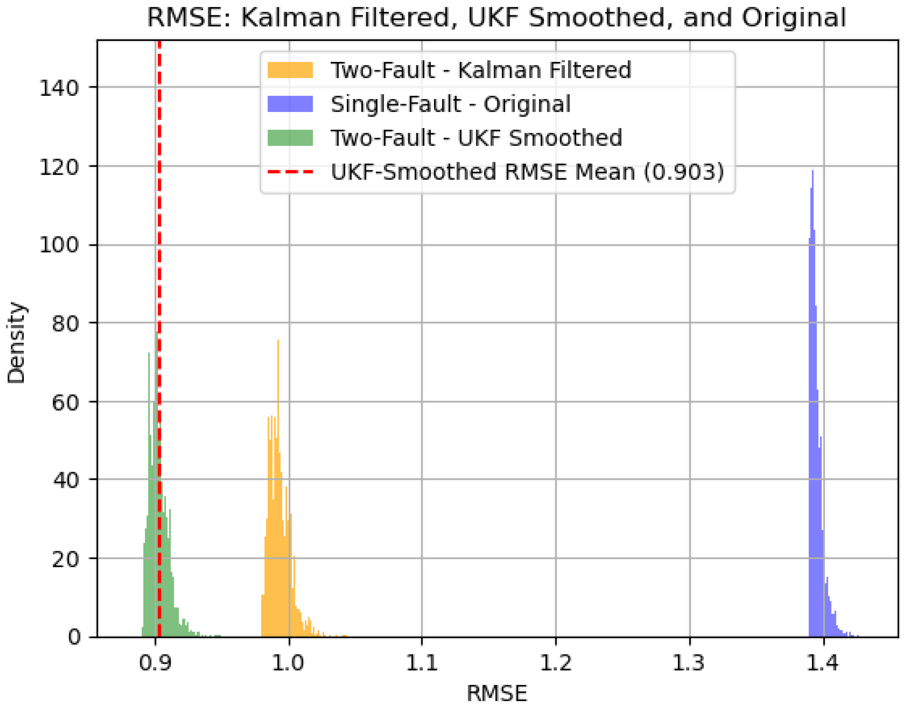
Figure 18.
Location of the Salton Sea relative to the southern end of the SAF (see Figure 1). The shadowed area north of the lake represents the SAF. The Salton Sea formed in 1905 due to flooding from a failed irrigation project.
Figure 18.
Location of the Salton Sea relative to the southern end of the SAF (see Figure 1). The shadowed area north of the lake represents the SAF. The Salton Sea formed in 1905 due to flooding from a failed irrigation project.
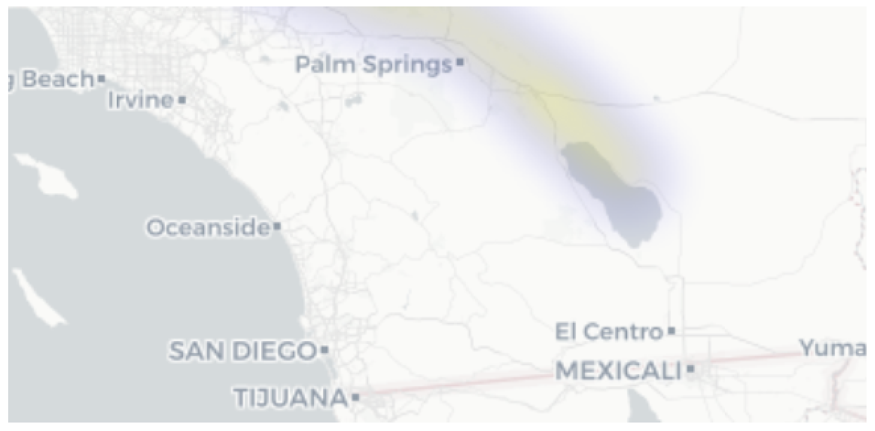
Figure 19.
The share and recorded causes of anthropogenic earthquakes.Raw data can be found in Human Induced Earthquake Database (Hiquake) [33]. Oil and Gas operations amount to ∼ 43% of seismic events induced by humans.
Figure 19.
The share and recorded causes of anthropogenic earthquakes.Raw data can be found in Human Induced Earthquake Database (Hiquake) [33]. Oil and Gas operations amount to ∼ 43% of seismic events induced by humans.
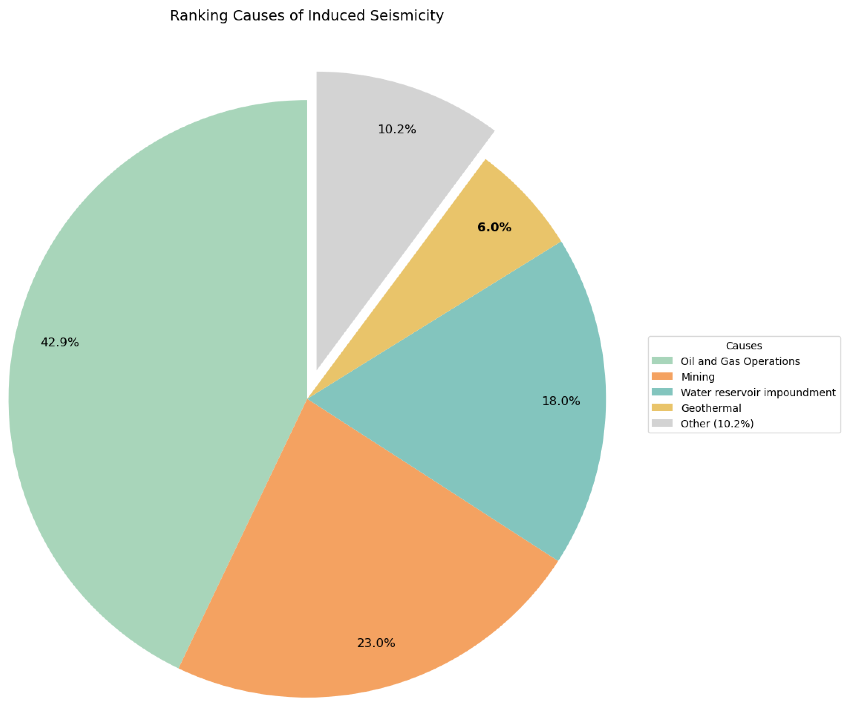
Figure 20.
Map of active or potential CCS operations in the United States, with Oklahoma particularly vulnerable. CO2 pipelines and induced seismicity pose risks to communities and seal integrity. Adapted from [38].
Figure 20.
Map of active or potential CCS operations in the United States, with Oklahoma particularly vulnerable. CO2 pipelines and induced seismicity pose risks to communities and seal integrity. Adapted from [38].
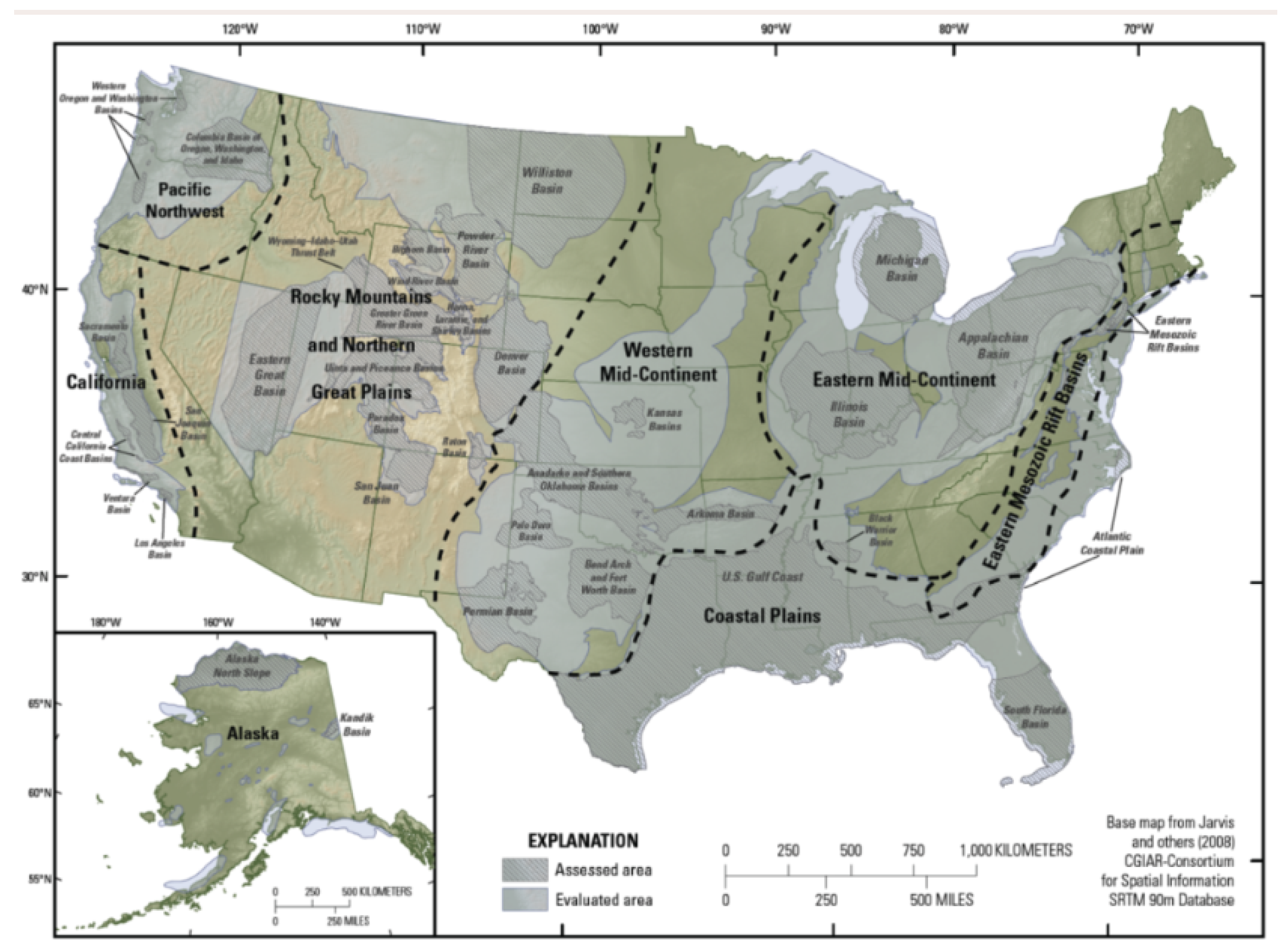
Figure 21.
The correlation between variables of concern on Earth, over a few decades (1959-2020) with each data point corresponding to one year, with as a hue, increasing every year. Higher concentrations (Filtered annual data from Keeling et. al. [42]) are correlated with higher Sea Levels (As reported by Church 2011 and University Of Hawaii Sea Level Center) [43,45] and higher temperature anomalies (Data from: Met Office H. C. [44]).
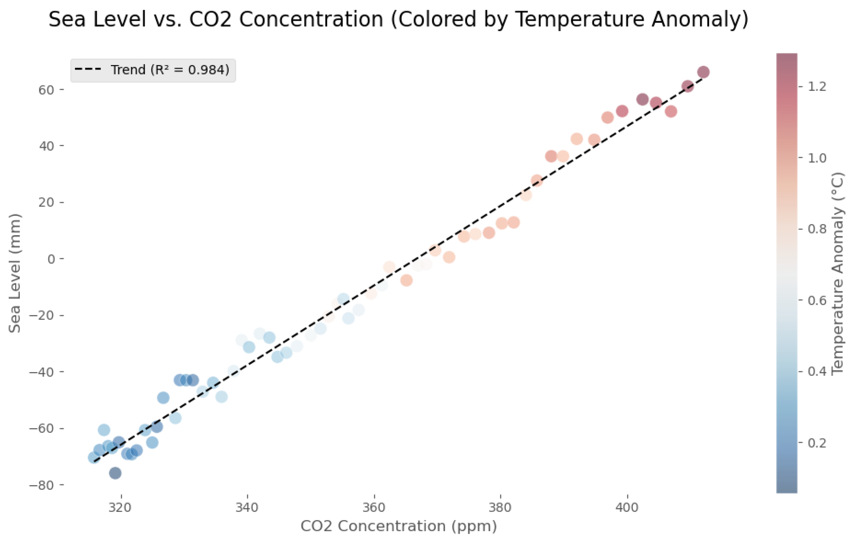

Table 1.
Single-fault model parameters with uncertainties. Velocities are in mm/year; depth and x are in km.
Table 1.
Single-fault model parameters with uncertainties. Velocities are in mm/year; depth and x are in km.
| 45.5 ± 0.6 | |
| 18.3 ± 0.4 | |
| D | 36 ± 1.1 |
Table 2.
Two-fault model parameters with uncertainties. Velocities are in mm/year; depth and x are in km.
Table 2.
Two-fault model parameters with uncertainties. Velocities are in mm/year; depth and x are in km.
| 23 ± 1 | |
| 14 ± 1 | |
| - | 0.4 ± 0.8 |
| 49 ± 1 | |
| 14 ± 1 | |
| 12 ± 1 |
Disclaimer/Publisher’s Note: The statements, opinions and data contained in all publications are solely those of the individual author(s) and contributor(s) and not of MDPI and/or the editor(s). MDPI and/or the editor(s) disclaim responsibility for any injury to people or property resulting from any ideas, methods, instructions or products referred to in the content. |
© 2025 by the authors. Licensee MDPI, Basel, Switzerland. This article is an open access article distributed under the terms and conditions of the Creative Commons Attribution (CC BY) license (http://creativecommons.org/licenses/by/4.0/).
Copyright: This open access article is published under a Creative Commons CC BY 4.0 license, which permit the free download, distribution, and reuse, provided that the author and preprint are cited in any reuse.


