
Submitted:
06 October 2025
Posted:
07 October 2025
You are already at the latest version
Abstract
Utilizing an asperity model, this research thoroughly simulates 3D seismic wave propagation to assess the 2016 Kumamoto earthquake. The research employs finite difference methods (FDM) to solve the 3D wave propagation equations incorporating realistic subsurface geological data and slip distributions from the Kumamoto active fault system. The simulation domain covers a 15 km × 12 km subsection of the fault plane, discretized into 250 m³ grid cells, resulting in a 48 × 60 mesh for numerical computation. The model utilized 800 iterative cycles to generate complete ground velocity time histories for an 8 second duration at numerous receiver locations. The results show that the x-direction component has the highest amplitude at station KMMH16, with seismic activity beginning around 3.5 seconds and rising around 5.9 seconds. The timing and intensity of the shaking differed greatly from one location to another primarily based on how far each site was from the fault and the direction in which it was located. This study advances our knowledge of earthquake source mechanics and helps to improve seismic hazard assessment and mitigation techniques by offering crucial insights into the intricacies of seismic wave propagation across heterogeneous media. The study clarifies the complex process of seismic waves propagating across various mediums which advances our knowledge of earthquake dynamics and enhances seismic risk assessment and mitigation strategies.
Keywords:
seismic wave propagation
; finite difference method
; asperity model
; Kumamoto earthquake
; ground motion simulation
; 3D numerical modeling
1. Introduction
The forecasting of seismic events and the simulation of ground vibrations remain substantial obstacles in the areas of geophysics and seismology. The catastrophic impacts of significant seismic events, exemplified by the 2016 Kumamoto earthquake in Japan, underscore the paramount importance of deciphering the mechanisms behind seismic wave propagation to advance hazard mitigation and risk evaluation strategies (Asano & Iwata, 2016; Kubo et al., 2016). Initiated on April 14, 2016, the Kumamoto earthquake sequence yielded invaluable datasets for examining intricate fault rupture dynamics and their consequent ground shaking patterns (Yoshida et al., 2016).
The numerical simulation of seismic wave propagation has been revolutionized in recent decades due to remarkable improvements in computational resources and advances in complex modeling techniques (Moczo et al., 2007; Kristek & Moczo, 2003). Among numerical techniques, the finite difference method (FDM) has become a predominant tool for simulating elastic wave behavior in complex geological environments (Virieux, 1986; Graves, 1996). Renowned for its computational efficacy and adaptability in addressing subsurface heterogeneity, this approach is especially well-suited for large-scale earthquake simulations (Olsen, 2000; Pitarka, 1999).The integration of asperity models into earthquake source characterization has gained substantial attention following their initial conceptualization by Kanamori (1981) and later enhancements by Somerville et al. (1999). These asperities refer to localized zones of concentrated stress on fault planes that significantly influence the release of seismic energy during rupture episodes (Madariaga, 1976; Das & Aki, 1977). Precise characterization of the spatial distribution and properties of asperities is essential for reliable ground motion estimation and informed seismic hazard analysis (Irikura & Miyake, 2001; Miyake et al., 2003).
The 2016 Kumamoto earthquake served as a pivotal case for analyzing intricate fault systems and their associated rupture dynamics. The magnitude 7.0 principal earthquake, which fractured the Futagawa fault network, was subsequently followed by a comprehensive succession of secondary tremors that illuminated the fault system’s intricate structural configuration (Shirahama et al., 2016). Documented seismic oscillations demonstrated substantial geographic heterogeneity in vibration magnitude, emphasizing the pivotal influence of localized geological characteristics and seismic source attributes in governing seismic wave transmission dynamics (Kawase et al., 2017).Prior research has confirmed the efficacy of three-dimensional numerical simulations in replicating observed ground motions from significant earthquakes. For instance, Graves & Pitarka (2010) accurately reproduced ground shaking from the 1994 Northridge event using a 3D finite-difference method, and Taborda & Bielak (2011) performed large-scale simulations of the 2008 Chino Hills earthquake. These investigations laid the groundwork for high-fidelity earthquake modeling and affirmed the reliability of numerical techniques in forecasting ground motion attributes. The incorporation of realistic geological structures into seismic wave simulations has demonstrated a significant improvement in the precision of strong ground motion forecasts (Olsen & Archuleta, 1996; Frankel & Vidale, 1992). Subsurface velocity configurations, especially sedimentary basins and sharp velocity gradients are known to amplify seismic waves and prolong strong shaking (Graves & Wald, 2001; Day et al., 2005). The Kumamoto area’s geologically complex environment—marked by intersecting fault networks and a heterogeneous crustal structure—offers an exemplary setting to examine these phenomena in detail.
Boundary conditions play a crucial role in numerical wave propagation simulations. The Clayton & Engquist (1977) absorbing boundary condition has been widely adopted to minimize artificial reflections from model boundaries. Subsequent developments, including perfectly matched layers (PML) by Berenger (1994) and improved absorbing conditions by Higdon (1987), have further enhanced the accuracy of numerical simulations by effectively suppressing spurious reflections. The verification of computational models against empirical ground motion observations is fundamental for affirming the reliability of simulation methodologies. Investigations by Aagaard et al. (2008) and Taborda et al. (2016) have underscored the necessity of rigorous validation incorporating diverse strong-motion metrics, including peak ground acceleration, velocity, and spectral characteristics. Such validation efforts are crucial for advancing the state-of-the-art in earthquake simulation and ensuring the reliability of predictions for engineering applications. Progress in high-performance computing has facilitated the development of increasingly sophisticated earthquake simulations, achieving unprecedented levels of spatial and temporal detail (Cui et al., 2010; Ichimura et al., 2014). These technological advancements have created novel opportunities for intricate analyses of seismic source mechanisms and their resultant ground shaking. Leveraging these developments, the current investigation provides critical insights into the 2016 Kumamoto event through a comprehensive three-dimensional numerical modeling framework.
2. Description of the Issue
The objective in this assignment is to calculate earthquake waveforms using an asperity model of an active fault. This involves defining the asperity area and specifying the slip distribution along the x and y directions. We will then apply the 3D wave propagation equation, along with relevant initial and boundary conditions, to simulate the resultant earthquake waveform in three dimensions (x, y, and z). Data pertaining to the rupture and soil profile of the Kumamoto earthquake (April 14, 2016) will be utilized. Successful completion of this assignment will deepen our insight into earthquake propagation mechanisms within the Earth’s crust and the influence of geological stratification and asperity zones on seismic waveform characteristics, which is critical for improving earthquake forecasting and impact reduction efforts.
2.1. Wave Propagation in 3-D
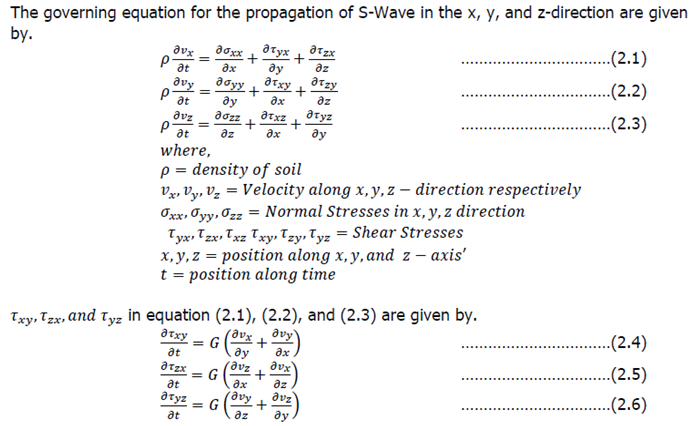
where,
𝐺 = 𝑆ℎ𝑒𝑎𝑟 𝑀𝑜𝑑𝑢𝑙𝑢𝑠 𝑜𝑓 𝑠𝑜𝑖𝑙
To understand and simulate the propagation of S-waves, we need to solve equations (2.1) to (2.6). To solve these differential equations, we will employ the Finite Difference Method (FDM) using Fortran Program. This method involves discretizing the soil system in both space (along the x, y, z-axis) and time (along the t-axis). By doing so, we transform the continuous domain into a grid of discrete points, making the equations solvable using numerical methods. This approach allows us to approximate the behavior of S-waves in the soil system over time.
By utilizing Equations (2.1) and (2.6), and applying initial and Boundary Condition, we can calculate the Velocity and Shear Stress at all (x, y, z, t) grid points.
2.2. Initial Condition
At the onset (t=0), the values of Shear Stress and Velocity at all points along the x, y, and z-axis are set to zero. This represents a state of equilibrium before the propagation of the earthquake wave begins.
2.3. Boundary Condition
When solving the differential equations that govern wave propagation, it’s impractical to model the entire Earth. Instead, we focus on a specific section of the physical domain. However, this approach can lead to disturbances in the calculated results due to reflections from the artificial boundary. To mitigate this, we utilize an absorbing boundary condition, as proposed by Clayton and Engquest in 1977.
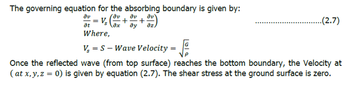
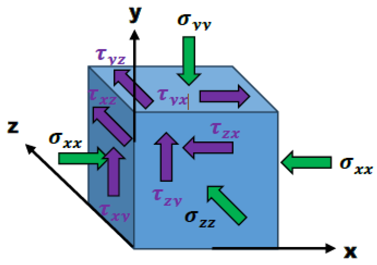
Figure 1.
Discrete 3D-Block of earth crust showing stresses.
3. Subsurface Data
The soil profile data relevant to the Kumamoto Active Fault, presented in Table 1, will be utilized for this assignment. Although the complete dataset includes parameters like Depth, P-wave Velocity, S-wave Velocity, and Density, this study will specifically focus on Soil Depth, S-wave Velocity, and Density. These three parameters are crucial for accurately simulating seismic wave propagation through the soil.
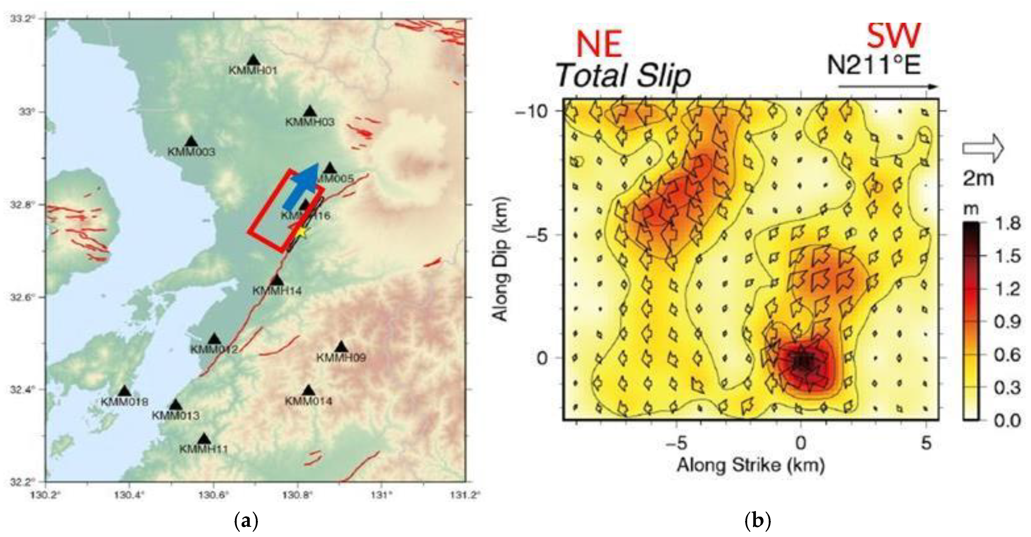
4. Kumamoto’s Active Geological Fault
The Kumamoto Active Fault stretches approximately 30 km in a SW-NE direction, extending approximately 21 km deep. During the 2016 Kumamoto Earthquake, it exhibited significant displacement, with a maximum slip of ~1.8 meters. Figures 2 (a& b) depict the fault’s orientation and the relative movement between the NW and SE blocks, using color scales and arrows to indicate slip magnitude and direction. For this assignment, an asperity area must be modeled, with prescribed x-direction (fault-parallel) and y-direction (vertical) movements mirroring the observed slip patterns. This simulation aims to enhance understanding of fault dynamics during seismic events.
Figure 2.
a) Active Fault in Kumamoto; b) Movement of NW block relative to SE block.
5. Slip Data
While the full fault measures 30 km × 21 km, computational constraints limit our study to a 15 km (length) × 12 km (depth) subsection in figure. This region is discretized into 250 m³ grid cells, yielding a 48 × 60 mesh for numerical simulation
Slip data –X
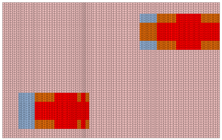
Slip Data –Y
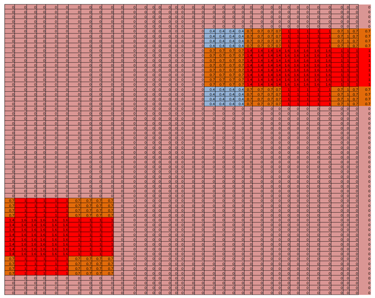
We focus on a particular high-stress zone (asperity) of the fault, shown in Figure 3’s 3D diagram, and determine how much it moves horizontally (x) and vertically (y). Figure 4 uses colors to show these movements, while another illustration displays the combined overall slip.
The slip data regions have been roughly delineated, as illustrated in the figure above. For simplicity, the data has been grouped into seven categories based on slip magnitude, as specified. The slip direction is indicated by a positive Y-component (downward) near the top asperity and a negative Y-component (upward) around the hypocenter. The slip data was successfully recreated in Microsoft Excel, with X-axis and Y-axis values stored in separate sheets. This structure mirrors the ‘rupt.data’ file format, where datasets correspond to dip divisions and series represent strike divisions. To align with the required trend, the Excel data was then converted into a .txt file.
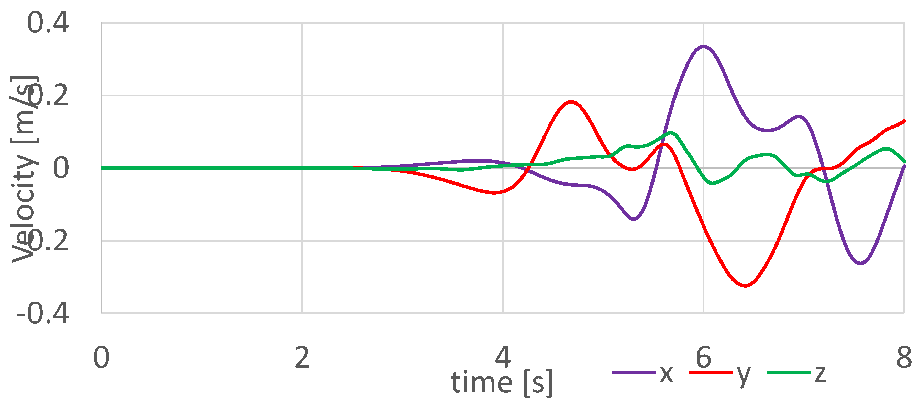
6. Computed Ground Motion at Location KMMH16
The Excel file was utilized to create a waveform representation at KMMH16. This waveform illustrates the ground velocity responses in the Vx (purple), Vy (red), and Vz (green) directions, corresponding to the three columns of the ‘KMMH16.data’ file. The calculations were performed over a total duration of 8 seconds, comprising 800 simulation loops.
Upon analyzing the graph, it becomes evident that the location begins to experience seismic activity at approximately 3.5 seconds, with notable shaking intensifying around 5.9 seconds. Among the three components, the x-direction (Vx) exhibits the largest amplitude, indicating that the strongest ground motion at KMMH16 occurs along the x-axis.
Figure 5.
Waveform at KMMH16 (calculated by my data with the help of slipx and slip y data).
7. Calculated Waveform at different points
We have also calculated the waveform at 4 other different points. The position of these points is depicted in Table 2. Point-1 and Point-2 lie in one line along z-axis, Point-2,3,4 lie in another line along x-axis, and Point-4,5 lie in one line along y-axis. These points were selected to compare the waveform in different directions.
Figure 6 presents the waveforms computed at Points 1 and 2, which are positioned along the z-axis. Point 1 is situated farther from the fault plane in the z-direction. An interesting observation from the figure is that the waveforms at both points commence simultaneously at approximately 3 seconds. However, the amplitude at Point 1, which is farther from the fault plane, is noticeably lower than that at Point 2, which is closer to the fault plane.
Figure 7 illustrates the waveforms computed at Points 2, 3, and 4, all of which are aligned along the x-axis. Point 2 is positioned to the left of Point A, while Point 4 is to the right. The waveform depicted in the figure reveals a shift in the initiation of the waveform from left to right. Specifically, the waveform at Point 2 begins at 3 seconds, and as we move in the positive x-direction, the waveform at Point 4 initiates at around 4.2 seconds. While comparing the amplitudes, it decreases initially as we move towards Point A, followed by an increase.
Figure 8 displays the waveforms computed at Points 4 and 5, which are arranged along the y-axis. The figure indicates that the waveform initiates first at depth. Furthermore, the amplitude of the waveform exhibits an increasing trend towards the ground surface.
Conclusions
This study successfully implemented a 3D finite difference numerical model to simulate seismic wave propagation from the 2016 Kumamoto earthquake based on an asperity model of the fault rupture. The combination of a defined, non-uniform slip pattern (across both the fault’s length and depth) with a detailed, layered subsurface model for the Kumamoto area enabled a physically realistic numerical representation of powerful seismic waves. The implementation of starting parameters (structural balance) and Clayton-Engquist energy-absorbing boundary constraints guaranteed a robust and precise computational result. The analysis of computed waveforms at multiple points in the domain yielded significant insights into wave propagation phenomena:
- Wave Initiation and Amplitude with Distance (Z-axis): Waveforms initiated simultaneously at different depths, confirming the source origin, but amplitudes notably decreased with increasing distance from the fault plane, illustrating geometric spreading and inelastic attenuation.
- Directivity and Propagation (X-axis): A clear time-shift in the initiation of shaking was observed along the strike direction, a characteristic signature of rupture directivity, where energy is focused in the direction of rupture propagation.
- Site Effects and Amplification (Y-axis): The increase in waveform amplitude towards the ground surface (Point 5 vs. Point 4) highlights the effect of impedance contrasts in the soil layers, leading to seismic amplification, a critical factor in seismic hazard assessment.
The simulation at the specific location KMMH16 correctly identified the x-component (Vx) as the most dominant, aligning with expectations from the fault’s mechanism and orientation. The timing of the wave arrival (~3.5 s) and the peak shaking (~5.9 s) were also realistically captured. This approach provides a valuable framework for understanding earthquake dynamics and improving seismic risk mitigation strategies.
Recommendation
While this model provides a robust foundation, several advancements could enhance its realism and predictive power:
- Higher Resolution Simulation: Employing a finer computational grid (e.g., <100 m cells) would better resolve the high-frequency content of seismic waves and allow for a more detailed representation of slip heterogeneity and complex near-surface geology.
- Incorporation of Full Wavefield: Extending the model to simulate both P-waves and S-waves by using the full elastic wave equation would provide a more complete picture of the ground motion, particularly for near-field observations.
- Non-Linear Soil Behavior: For strong shaking near the source, soils behave non-linearly. Implementing constitutive models that account for this non-linear response and potential liquefaction would greatly improve accuracy in predicting extreme ground motions.
- Validation with Real Data: To ensure the model’s accuracy, the logical next step is to validate it against empirical records. This would involve a direct, quantitative comparison between the simulated ground motions such as those for station KMMH16 and the actual seismograms from the Kumamoto event. Such a comparison is essential for confirming the current parameters and identifying specific aspects of the model that could be refined.
- Dynamic Rupture Modeling: A significant advancement would be to transition from a kinematic model which assumes a fixed slip distribution, to a dynamic rupture approach. In a dynamic model, the earthquake’s breakage evolves naturally based on physical principles like friction and stress transfer. This shift is crucial for developing a more fundamental and comprehensive picture of how an earthquake starts and spreads.
- Broadband Simulation: Combining a low-frequency finite difference simulation with a high-frequency stochastic approach could efficiently generate broadband seismograms (0-10 Hz+) necessary for engineering applications.
- 3D Basin Effects: Modeling a more complex 3D sedimentary basin structure, rather than a 1D soil profile, to capture basin-edge effects and guided waves that can significantly amplify and prolong shaking.
References
- Aagaard, B. T., Hall, J. F., & Heaton, T. H. (2008). Characterization of near-source ground motions with earthquake simulations. Earthquake Spectra, 17(2), 177-207. [CrossRef]
- Asano, K., & Iwata, T. (2016). Source rupture processes of the foreshock and mainshock in the 2016 Kumamoto earthquake sequence estimated from the kinematic waveform inversion of strong motion data. Earth, Planets and Space, 68, 147. [CrossRef]
- Berenger, J. P. (1994). A perfectly matched layer for the absorption of electromagnetic waves. Journal of Computational Physics, 114(2), 185-200. [CrossRef]
- Clayton, R., & Engquist, B. (1977). Absorbing boundary conditions for acoustic and elastic wave equations. Bulletin of the Seismological Society of America, 67(6), 1529-1540. [CrossRef]
- Cui, Y., Olsen, K. B., Jordan, T. H., Lee, K., Zhou, J., Small, P., ... & Maechling, P. J. (2010). Scalable earthquake simulation on petascale supercomputers. Proceedings of the 2010 ACM/IEEE International Conference for High Performance Computing, 1-20.
- Das, S., & Aki, K. (1977). A numerical study of two-dimensional spontaneous rupture propagation. Geophysical Journal International, 50(3), 643-668. [CrossRef]
- Day, S. M., Graves, R. W., Bielak, J., Dreger, D., Larsen, S., Olsen, K. B., ... & Ramirez-Guzman, L. (2005). Model for basin effects on long-period response spectra in southern California. Earthquake Spectra, 21(2), 257-277.
- Frankel, A., & Vidale, J. (1992). A three-dimensional simulation of seismic waves in the Santa Clara Valley, California, from a Loma Prieta aftershock. Bulletin of the Seismological Society of America, 82(5), 2045-2074.
- Graves, R. W. (1996). Simulating seismic wave propagation in 3D elastic media using staggered-grid finite differences. Bulletin of the Seismological Society of America, 86(4), 1091-1106. [CrossRef]
- Graves, R., & Pitarka, A. (2010). Broadband ground-motion simulation using a hybrid approach. Bulletin of the Seismological Society of America, 100(5A), 2095-2123. [CrossRef]
- Graves, R. W., & Wald, D. J. (2001). Resolution analysis of finite fault source inversion using one-and three-dimensional Green’s functions: 1. Strong motions. Journal of Geophysical Research, 106(B5), 8745-8766.
- Higdon, R. L. (1987). Numerical absorbing boundary conditions for the wave equation. Mathematics of Computation, 49(179), 65-90.
- Ichimura, T., Fujita, K., Tanaka, S., Hori, M., Lalith, M., Shizawa, Y., & Kobayashi, H. (2014). Physics-based urban earthquake simulation enhanced by 10.7 BlnDOF × 30 K time-step unstructured FE non-linear seismic wave simulation. Proceedings of the International Conference for High Performance Computing, 15-26.
- Irikura, K., & Miyake, H. (2001). Prediction of strong ground motions for scenario earthquakes. Journal of Geography, 110(6), 849-875. [CrossRef]
- Kanamori, H. (1981). The nature of seismicity patterns before large earthquakes. Earthquake Prediction, 4, 1-19.
- Kawase, H., Matsuo, H., Nagashima, F., & Baoyintu, B. (2017). The cause of heavy damage concentration in downtown Mashiki inferred from observed data and field survey of the 2016 Kumamoto earthquake. Earth, Planets and Space, 69, 3. [CrossRef]
- Kristek, J., & Moczo, P. (2003). Seismic-wave propagation in viscoelastic media with material discontinuities: a 3D fourth-order staggered-grid finite-difference modeling. Bulletin of the Seismological Society of America, 93(5), 2273-2280.
- Kubo, H., Suzuki, W., Aoi, S., & Sekiguchi, H. (2016). Source rupture processes of the 2016 Kumamoto, Japan, earthquakes estimated from strongmotion waveforms. Earth, Planets and Space, 68, 161. [CrossRef]
- Madariaga, R. (1976). Dynamics of an expanding circular fault. Bulletin of the Seismological Society of America, 66(3), 639-666. [CrossRef]
- Miyake, H., Iwata, T., & Irikura, K. (2003). Source characterization for broadband ground-motion simulation: Kinematic heterogeneous source model and strong motion generation area. Bulletin of the Seismological Society of America, 93(6), 2531-2545.
- Moczo, P., Robertsson, J. O., & Eisner, L. (2007). The finite-difference time-domain method for modeling of seismic wave propagation. Advances in Wave Propagation in Heterogeneous Earth, 48, 421-516.
- Olsen, K. B. (2000). Site amplification in the Los Angeles basin from three-dimensional modeling of ground motion. Bulletin of the Seismological Society of America, 90(6B), S77-S94. [CrossRef]
- Olsen, K. B., & Archuleta, R. J. (1996). Three-dimensional simulation of earthquakes on the Los Angeles fault system. Bulletin of the Seismological Society of America, 86(3), 575-596. [CrossRef]
- Pitarka, A. (1999). 3D elastic finite-difference modeling of seismic motion using staggered grids with nonuniform spacing. Bulletin of the Seismological Society of America, 89(1), 54-68. [CrossRef]
- Shirahama, Y., Yoshida, M., Sueta, Y., Goto, H., Kapitulčinová, D., Nakata, T., ... & Chiba, T. (2016). Characteristics of the surface ruptures associated with the 2016 Kumamoto earthquake sequence, central Kyushu, Japan. Earth, Planets and Space, 68, 191.
- Somerville, P., Irikura, K., Graves, R., Sawada, S., Wald, D., Abrahamson, N., ... & Kramer, S. (1999). Characterizing crustal earthquake slip models for the prediction of strong ground motion. Seismological Research Letters, 70(1), 59-80. [CrossRef]
- Taborda, R., & Bielak, J. (2011). Large-scale earthquake simulation: computational seismology and complex engineering systems. Computing in Science & Engineering, 13(4), 14-26. [CrossRef]
- Taborda, R., Azizzadeh--Roodpish, S., Khoshnevis, N., & Cheng, K. (2016). Evaluation of the southern California seismic velocity models through simulation of recorded earthquakes. Geophysical Journal International, 205(3), 1342-1364. [CrossRef]
- Virieux, J. (1986). P-SV wave propagation in heterogeneous media: Velocity--stress finite--difference method. Geophysics, 51(4), 889-901. [CrossRef]
- Yoshida, S., Koketsu, K., Shibazaki, B., Sagiya, T., Kato, T., & Yoshida, Y. (2016). Joint inversion of near- and far-field waveforms and geodetic data for the rupture process of the 1995 Kobe earthquake. Journal of Physics of the Earth, 44(4), 437-454. [CrossRef]
Figure 3.
Fault Plane in 3D View.
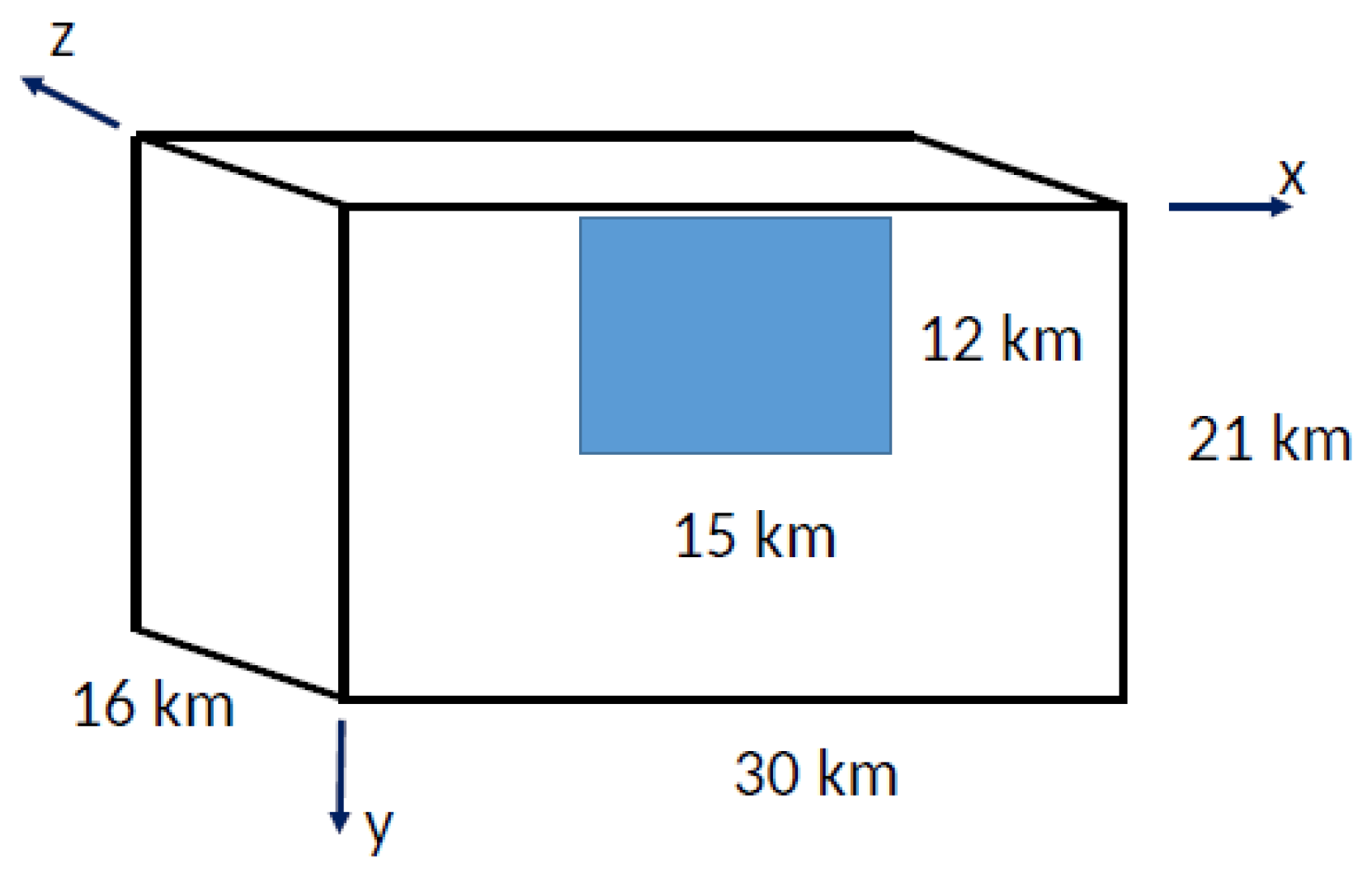
Figure 4.
Slip in X, and Y-direction.
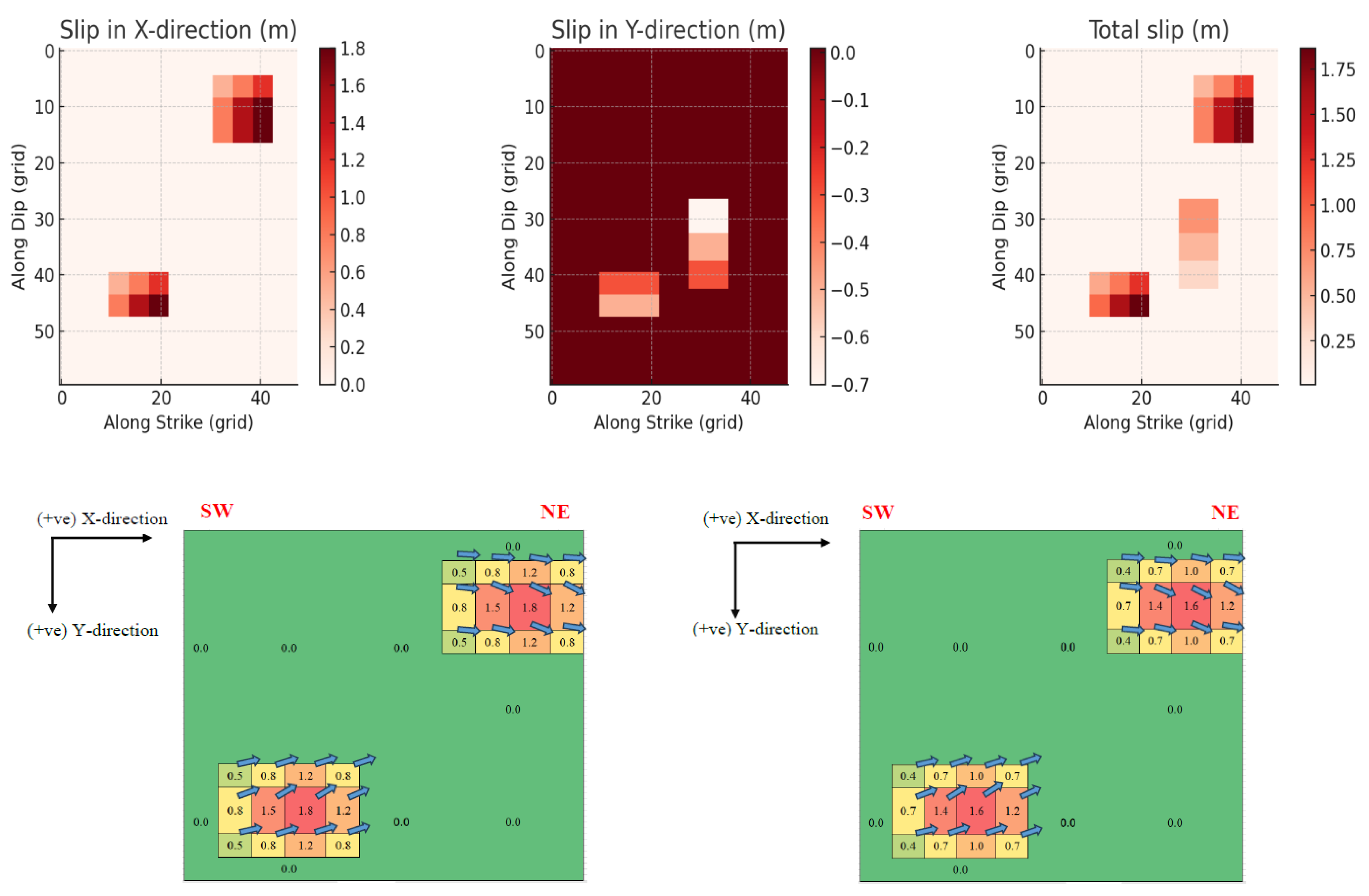
Figure 6.
Waveform at Point-1, and Point-2 Along Z-Axis with same X and Y Position.
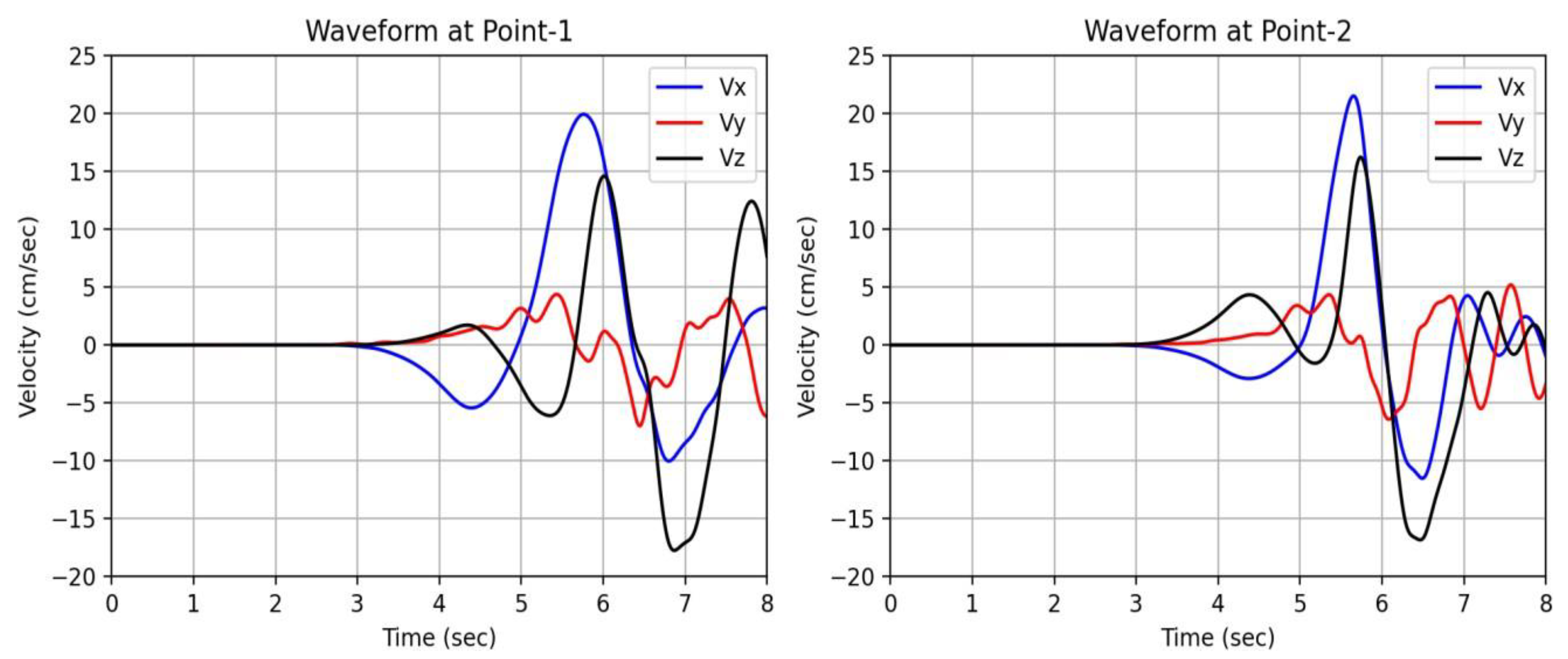
Figure 7.
Waveform at Point 2, 3, 4 along X-axis with same Y and Z Position.
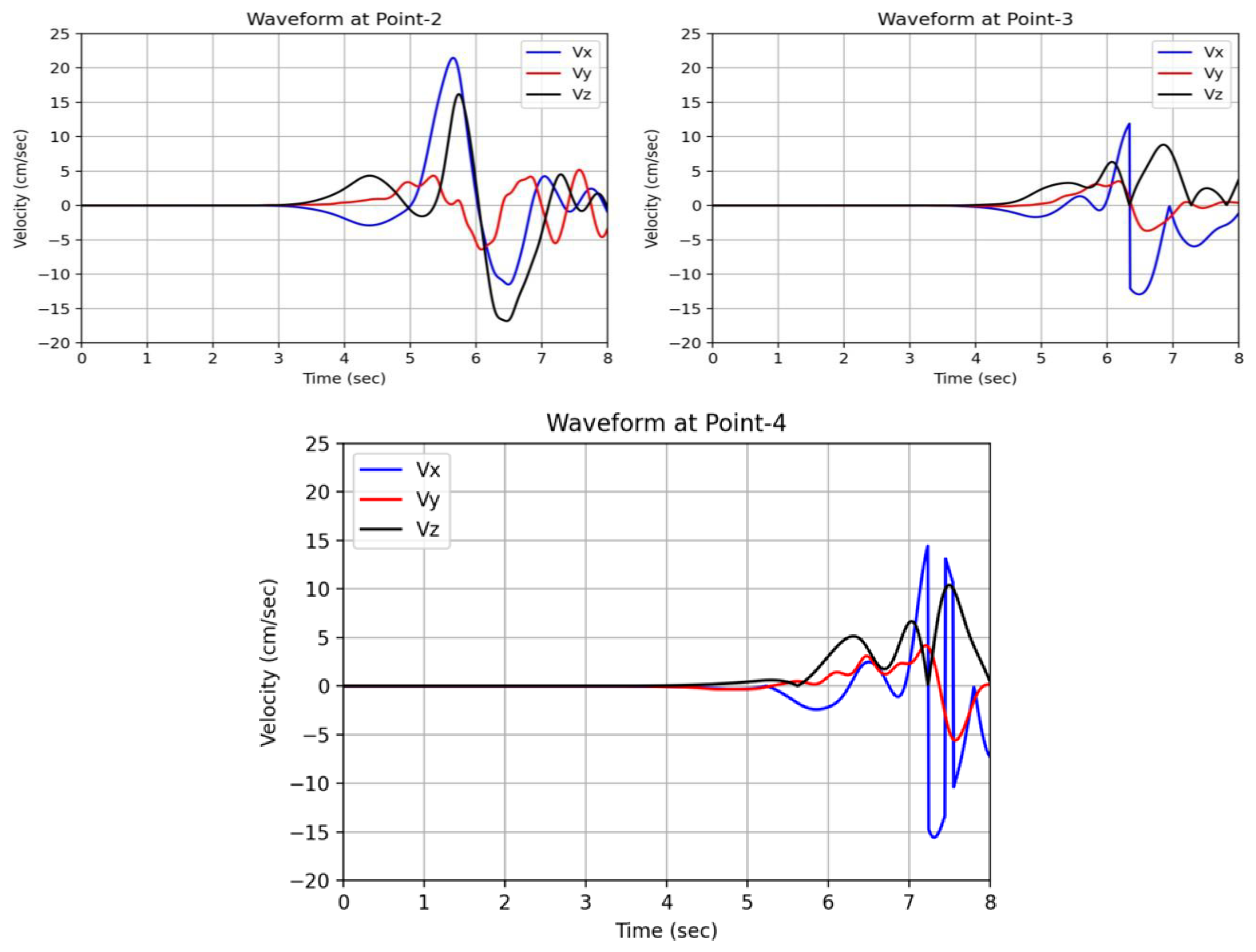
Figure 8.
Waveform at Point 4, and 5 along Y-axis with same X and Z Position.
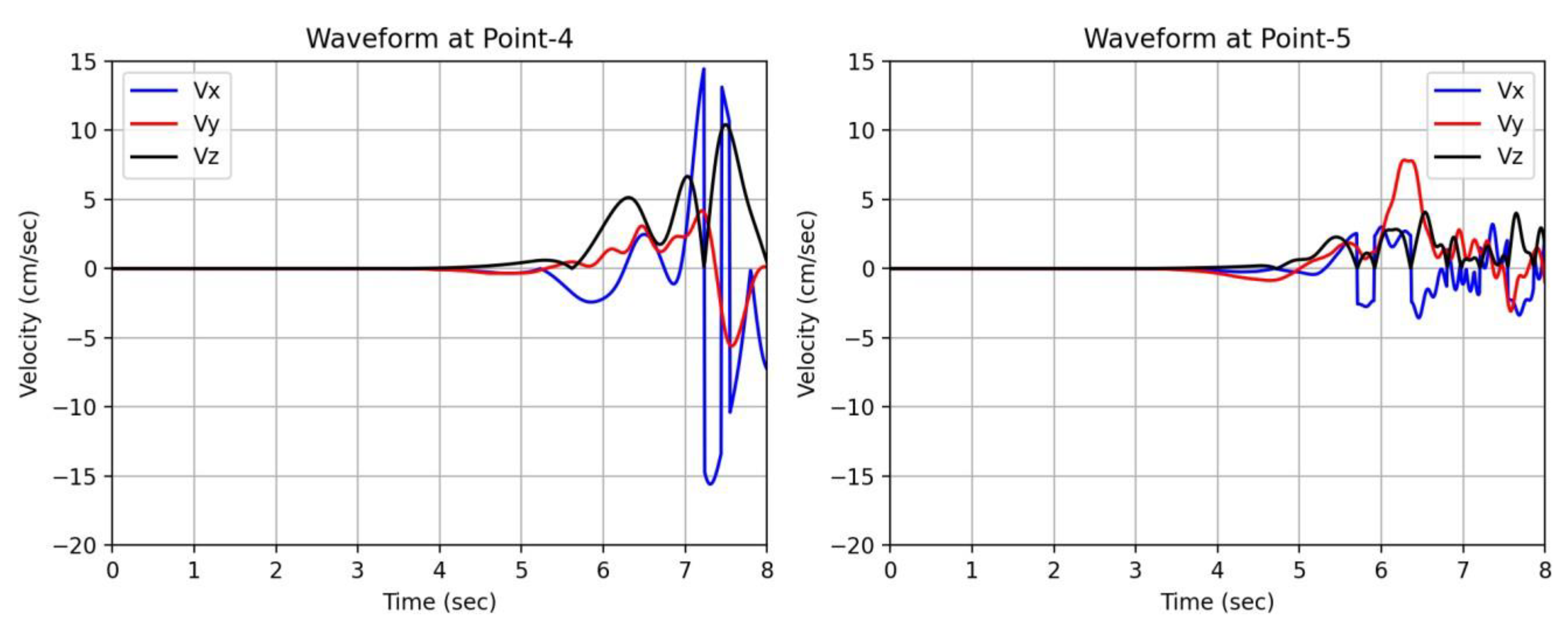

Table 1.
Caption.
| Depth (m) | P-Velocity (m/s) | S-Velocity (m/s) | Density (kg/m3) |
| 0-500 | 2000 | 600 | 2000 |
| 500-800 | 2500 | 1100 | 2150 |
| 800-1500 | 3600 | 2100 | 2350 |
| 1500-5000 | 5300 | 3100 | 2600 |
| 5000-30000 | 5800 | 3400 | 2700 |
| >30000 | 6400 | 3800 | 2800 |
Table 2.
Point Details.
|
Point Name |
Grid Position relative to point A | Spatial Location Relative to A | Remarks | ||||
| X (cell) | Y (cell) | Z (cell) | X (m) | Y (m) | Z (m) | ||
| Point-A | 0 | 0 | 0 | 0 | 0 | 0 | Reference |
| Point-1 | -15 | -2 | 10 | -3250 | -500 | 2500 | |
| Point-2 | -15 | -2 | 5 | -3250 | -500 | 1250 | KMMH16 |
| Point-3 | -1 | -2 | 5 | -250 | -500 | 1250 | |
| Point-4 | 13 | -2 | 5 | 3000 | -500 | 1250 | |
| Point-5 | 13 | -10 | 5 | 3000 | -2500 | 1250 | |
Disclaimer/Publisher’s Note: The statements, opinions and data contained in all publications are solely those of the individual author(s) and contributor(s) and not of MDPI and/or the editor(s). MDPI and/or the editor(s) disclaim responsibility for any injury to people or property resulting from any ideas, methods, instructions or products referred to in the content. |
© 2025 by the authors. Licensee MDPI, Basel, Switzerland. This article is an open access article distributed under the terms and conditions of the Creative Commons Attribution (CC BY) license (http://creativecommons.org/licenses/by/4.0/).
Copyright: This open access article is published under a Creative Commons CC BY 4.0 license, which permit the free download, distribution, and reuse, provided that the author and preprint are cited in any reuse.


