
Submitted:
23 January 2025
Posted:
24 January 2025
You are already at the latest version
Abstract
This study presents a comprehensive analysis of site effects in the highly seismic area of L'Aquila in central Italy, which has been conducted within the framework of a seismic microzonation project funded by the Abruzzo Region's Department of Government of the Territory and Environmental Policies. The project was aimed at best practice on the management of urban and land territory for seismic risk mitigation. Through the integration of detailed geophysical and geotechnical data with numerical modeling, we provide an accurate assessment of local seismic amplification. Two-dimensional numerical simulations using the LSR 2D code were performed on many representative geological sections to compute amplification factors for various period ranges. This case study allowed us to outline some key considerations for best practices in local seismic response analysis and seismic microzonation studies in Italy. Given the prevalence of 2D basin edge, buried morphology and topographic effects in Plio-Quaternary geologically complex intermontane basins in central Italy, as demonstrated in the LAB case study, use of two-dimensional models is suggested. In order to validate the numerical models and their associated spectra and AFs, is also suggested to compare transfer functions with HVSR microtremor measurements at control points along the studied sections.
Keywords:
site effects
; seismic amplification
; seismic microzonation
; 1D and 2D numerical modeling
; Plio-Quaternary sedimentary basin
; L'Aquila
; central Italy
1. Introduction
In Italy, Level 3 analysis involves a detailed representation of the local seismic response using a strictly quantitative technique to assess local seismic impacts. This technique relies on laboratory and site investigations, as well as the processing of analytical and/or numerical data. It is now well-known that, at a local site scale, the seismostratigraphic and topographic effect can induce the seismic wave amplification [Borcherdt 1970; Kramer 1996]. These phenomena are known as local seismic effects. It is easy to see how these effects have a significant impact on infrastructures and buildings [Bisch et al. 2012¸ CS.LL.PP. 2018]. Therefore, they need to be assessed for the best practice of seismic risk mitigation [SM Working Group 2008; Ansal et al. 2010; Aversa and Crespellani 2016]. Their evaluation is typically obtained through numerical simulations of seismic wave propagation and the estimation of the amplification factors (AFs) [Pergalani et al. 2020]. For a given period interval (e.g., 0.1 – 0.5 s), AF is the ratio between the average spectral acceleration (averaged over the period interval itself) measured at the ground surface and that measured on outcropping seismic bedrock, given the same seismic input. Modeling requires, as input, the geometry of the seismo-layers and their geotechnical and geophysical properties [Ciancimino et al. 2019]. These primarily include the depth of the seismic bedrock, the dip of the seismostratigraphic boundaries, Vs, and the dynamic behavior of each seismo-layer.
Investigating these local effects becomes especially challenging when the subsoil model and the dynamic properties of the seismo-layers are complex and deviate from typical patterns, such as not in the simplest case of flat, parallel layers where Vs increases with depth [Bard and Bouchon 1985; Lanzo and Silvestri 1999; Smerzini et al. 2011; Giallini et al. 2024].
The intermontane plains of central Italy, subject to a high seismicity, as evidenced by the 2009 L'Aquila earthquake (Mw 6.3) and 2016-17 central Italy seismic sequence (Mw 6.0 and 6.5), exhibit particularly complex geometries and geophysical and geotechnical characteristics [MS-AQ Working Group 2010; Evangelista et al. 2011; Lanzo et al. 2011; Monaco and Amoroso 2016¸ Alleanza et al. 2024]. These can be schematized as follows: (i) thin shallow seismo-layers with strong seismic impedance contrasts; (ii) sub-vertical or strongly inclined geological boundaries between different lithologies such as faults or erosion surfaces; (iii) inversions of seismo-layer velocities with depth; (iv) at least two or more seismic impedance contrasts at different depths; (v) buried paleomorphology of deep and shallow paleo-valleys; (vi) positive topographies such as ridges and hills; (vii) channelling of seismic waves within fault rocks; (viii) regolith of outcropping rock with Vs < 800 m/s; (ix) infilling basin deposits that instead show Vs > 800 m/s.
Therefore, for proper prevention and management of urban areas of central Italy, the study of local seismic effects plays a significant role, to the extent that numerous pilot projects on seismic microzonation and the study of local seismic effects have been carried out.
One of these was carried out in the areas of L'Aquila Municipality, following the near-source event of April 6th, 2009 [Chiarabba et al. 2009]. A portion of the results of this seismic microzonation project is presented in this work. It is focused on two western (Preturo-Sassa) and eastern (Bazzano-Monticchio) pilot areas of L'Aquila Municipality (Figure 1 and Figure 2).
This seismic microzonation project, aimed at best practice on the management of urban and land territory for seismic risk mitigation, was funded by the Abruzzo Region's Department of Government of the Territory and Environmental Policies - Civil Protection Risk Prevention Service.
The pilot areas of about 7 km2 are geologically situated within the L'Aquila intermontane basin, characterized by thick accumulations of coarse- and fine-grained sediments deposited during the Plio-Quaternary primarily in lacustrine, slope, and fluvial settings [Nocentini et al. 2017].
In compliance with the Italian Civil Protection Department's guidelines [SM Working Group 2008], the seismic microzonation project concluded with the production of numerical maps in which the AFs are reported. The AFs were calculated via 1D and 2D numerical simulations of local seismic response on fifteen 3500-5000 m long geological sections representative of the pilot areas. They were specifically elaborated within the seismic microzonation project via many borehole data. Furthermore, the geophysical and geotechnical properties of the seismo-layers represented in them were assigned based on many in-situ and lab investigations. Three-dimensional local seismic response simulations were not performed due to the complexity and inherent uncertainties associated with reconstructing the 3D subsurface structure. Additionally, the substantial computational demands required for modeling such large areas made this approach infeasible. The 2D modelling and the comparison between AFs and the related spectra obtained with 1D and 2D modelling permitted also to recognize several of the above-mentioned local seismic effects. In some cases, these could be reasonably predicted (e.g., the presence of thin shallow seismo-layers with strong seismic impedance contrasts), in other cases not (e.g., buried paleomorphology of deep paleo-valleys). Among the aims of the seismic microzonation project, we find proposals for warnings for the best practices of numerical simulations to estimate AFs used in seismic microzonation maps.
The results presented herein offer twofold utility, serving both speculative and practical purposes. On the one hand, the studied area provides an excellent natural laboratory exhibiting a complex geological and seismostratigraphic setting. Extensive field surveys and geophysical investigations, coupled with numerical simulations, have enabled a detailed reconstruction of the subsurface characteristics and local seismic response, so providing interesting insights into the factors controlling site-specific seismic amplification. On the other hand, this study provides a detailed reconstruction of ground stratigraphic and geotechnical features, as well as of the local seismic response, over several sections in the area, serving as valuable tools for seismic risk mitigation and future studies in this area.
2. Geological Background
The Plio-Quaternary extensional tectonic regime in central Italy, characterized by SW-dipping normal faults, has shaped the landscape, forming graben structures and intermontane basins such as the L'Aquila Basin [Faure Walker et al. 2021]. This latter has been filled with various detrital deposits since the Upper Pliocene (3.6 million years) to the present [Cavinato and De Celles 1999; Nocentini et al. 2017]. The ongoing activity of these faults poses a significant seismic hazard to the region, with the potential for moderate to strong earthquakes (awaited maximum magnitudes of up to 6.5-7) [Devoti et al. 2010; Pondrelli et al. 2006; Galadini and Galli 2000].
The L'Aquila Basin sedimentary record begins in the upper Piacenzian (3.0–2.6 Myr) with the deposition of breccias and conglomerates: Colle Cantaro–Cave Formation in the Preturo–Sassa area and Valle Orsa Formation and Valle Valiano Formation in Bazzano–Monticchio area (all1). These units were followed, via an unconformity boundary above all in the Preturo–Sassa area, by Calabrian (1.8–0.8 Myr) alluvial floodplain silts and sands (Madonna della Strada Synthem, all2). A significant hiatus, marked by an unconformity, separates all2 from the overlying Middle Pleistocene (0.8–0.12 Myr) alluvial fan and plain deposits of the Fosso Genzano Synthem composed by gravels and sands (at1).
The L'Aquila historic center is situated on a hill composed of late Middle Pleistocene (0.3–0.12 Myr) calcareous breccias (Colle Macchione-L’Aquila Synthem, dbf). These breccias overlie the older units all2 and at1 and the Meso–Cenozoic substratum [Sciortino et al. 2024a; 2024b]. The surrounding L'Aquila Basin landscape is lastly characterized by recent slope (fal) and colluvial (col) deposits, as well as the alluvial deposits of the Aterno River and its tributaries such as the Raio Stream (all3).
In the cross-sections reported in Figure 3 the geological relationships of the main units are shown. The Plio-Quaternary L’Aquila basin-cover units are ant, fra, col, at1, all3 S, all3 G, all2, and all1. The units UAP and UAM refer to the terrigenous bedrock; the unit CCD to the carbonate bedrock.
The above-mentioned units of the Preturo-Sassa and Bazzano-Monticchio areas are summarized in Table 1 [Tallini et al., 2024]. The unit codes adopted in the modeling sections are based on the Abruzzo Seismic Microzonation Working Group (2012).
3. Materials and Methods
3.1. Geotechnical and Geophysical Database
A database was set up for storing and managing borehole, geotechnical and geophysical data, and seismic microzonation numerical maps via (i) QGIS (version 3.30.3-‘s-Hertogenbosch) and (ii) the plugin “mzs-tools” by CNR-IGAG (https://github.com/CNR-IGAG/mzs-tools, accessed on 15 November 2024) [Cosentino et al. 2022]. The stored investigations were carried out for the anti-seismic urban reconstruction activities following the April 6, L’Aquila earthquake. Furthermore, ad hoc investigations (above all 2D microtremor arrays, boreholes, static cone penetration tests, ERTs) were performed within the activities of the seismic microzonation project. They were placed in significative sites of the pilot areas for investigating the subsoil model and the coseismic instabilities [Tallini et al. 2024].
Several borehole logs, geotechnical and geophysical surveys, were stored in the QGIS database (Table 2). As an example, in Figure 4 and Figure 5 the investigations and the resonance frequency map obtained through the QGIS database are shown. The maps highilights the high density of data used within the seismic microzonation project. In the Sassa area, crossed by section A-A', numerous microtremor measurements have highlighted resonance frequency values between 2 and 4 Hz.
3.2. Geological Sections
Seven and eight 3500-5000 m-long geological sections were elaborated at fine scale (1:5000) in the Preturo-Sassa and Bazzano-Monticchio pilot areas, respectively and 1D and 2D simulations were conducted on them. The sections were designed to intersect the significant geological features within the pilot areas, such as fault lines, terrace scarps, landslides, and anthropic deposits and most microzones. The microzone is defined as a geologically homogeneous zone susceptible to local amplification or/and to coseimic instabilities at fine - 1:5000 scale [SM Working Group 2008]). Additionally, the sections were placed near the geophysical investigation sites, primarily microtremor measurements and down-hole tests, as well as boreholes, to enhance the accuracy of the subsoil model. The sections start and end at least 400 m outside their extremes located into the seismic bedrock for minimizing in the simulations the edge effects caused by the lateral dispersion of seismic energy [Tallini et al. 2024]. The seismic bedrock is defined by the Italian technical standards for construction [CS.LL.PP. 2018] as having the shear wave velocity Vs > 800 m/s. Furthermore, to validate simulations of possible 2D phenomena arising from seismic directionality, orthogonal sections have been elaborated and 2D simulated [Lanzo and Silvestri 1999].
In this paper we discuss in detail five of these sections (sections A-A’, B-B’, C-C’ in Figure 1, and D-D’, E-E’ in Figure 2), as they provide compelling examples of local seismic effects related to 2D subsurface conditions. Sections A-A’, B-B’, C-C’, and D-D’ exhibit both conditions well approximated by one-dimensional stratigraphy and scenarios where the influence of two-dimensional subsurface geometry (2D effects) is significant. They also point out how distinct sites with identical stratigraphy but varying seismic layer thicknesses can exhibit differing amplification factors. Section E-E’, conversely, presents a noteworthy case where seismic amplification, albeit moderate, is observed on outcropping bedrock.
3.3. Geotechnical and Geophysical Characteristics of the Units
The geophysical and geotechnical parameters of the units listed in Table 3 and used for numerical simulations represent average values derived from extensive on-site investigations conducted across the L'Aquila Basin area [e.g., MS-AQ Working Group 2010; Monaco et al. 2012; de Magistris et al. 2013] or stored in the QGIS database (Table 3).
Examples of results of cross-hole prospections conducted by previous studies [Del Monaco et al. 2013; Chiaradonna et al. 2024] in representative locations of the study areas (cross-hole A and B in Figure 1 and Figure 2, respectively) are illustrated in Figure 6, in terms of shear wave velocities Vs measured for the main seismo-layers. Finally, in the two studied areas no cases of inversion of seismo-layer velocities with depth were found.
3.4. Seismic Input
The Italian technical standards for construction, [CS.LL.PP. 2018] recommends using seven appropriately selected natural accelerograms as input signals for numerical simulations. This involved running each 1D and 2D simulation seven times, once for each accelerogram, and subsequently averaging the resulting seven spectra to obtain the final output. In accordance with the mentioned technical standards, seven natural accelerograms were selected from the online REXELite database (https://itaca.mi.ingv.it/ItacaNet_40/#/rexel, accessed on November 15, 2024) [Sgobba et al. 2019] using a spectrum matching approach. REXELite is a simplified version of the Rexel database [Iervolino et al. 2009].
The seven seismic events were selected based on the following criteria: (i) magnitude (Mw or Ml) between 5.5 and 7; (ii) extensional fault focal mechanism; (iii) epicentral distance of 0-30 km, and (iv) recording site on seismic bedrock.
The seven inputs are acceptable for the simulations if the average value, calculated for each frequency or period, is compatible with a target spectrum. Following the Italian regulation [CS.LL.PP. 2018], the upper and lower tolerance between the average value and the target spectrum is equal to 30% and 10%, respectively, in the 0.1-1.1 second period range. The target response spectrum used for L’Aquila (latitude: 42.377; longitude: 13.310) is associated with a reference earthquake having a 475-year return period on seismic bedrock (Vs > 800 m/s), assuming horizontal topography and 5% damping. This spectrum is automatically calculated by REXELite when querying the database.
3.5. Approach to Simulation of Real Soil Behavior
Soils subjected to cyclical loading exhibit nonlinear elastic dissipative behavior, manifested as hysteresis loops in the shear stress (τ) versus shear strain (γ) plane. This nonlinear elastic behavior cannot be neglected in earthquake related strain conditions and can be effectively represented using a Kelvin-Voigt viscoelastic model [Kramer 1996; Yoshida 2015]. Numerical analyses addressing soil nonlinearity typically employ one of two approaches [Kramer 1996; Yoshida 2015]: (1) the equivalent linear method or (2) the incremental nonlinear method. The equivalent linear method involves a sequence of linear analyses, where soil nonlinearity is approximated using the secant shear modulus (G), defined as the ratio τ/γ for an opportunely chosen γ value, and the damping ratio (D), which is proportional to the area enclosed by the hysteresis loop (i.e., to the energy loss at each loop).
Conversely, the incremental nonlinear method entails a step-by-step time-domain integration of the motion equations based on a nonlinear Kelvin-Voigt soil constitutive model. This approach, however, presents certain limitations. For instance, established linear analysis techniques, such as the superposition principle, transfer functions, and Fourier analysis, become inapplicable. Moreover, solving nonlinear differential equations is inherently more complex than solving linear ones. Numerical solutions of these nonlinear equations can frequently encounter convergence issues, necessitating numerous iterations. Consequently, a fully nonlinear treatment introduces greater algorithmic complexity and often a substantial computational demand, making codes implementing this approach more difficult to develop, validate, and maintain, resulting in increased costs. To mitigate these challenges, many simulation codes adopt the equivalent linear approach. This method involves integrating the dynamic motion equations (in the time or frequency domain), driven by an input accelerogram representing the target earthquake, using initial estimates for the elastic moduli (usually, the maximum value, denoted by G0, deduced by in situ Vs measurements) and damping ratios [Kramer 1996]. This integration yields the maximum strain (γMax) at each point within the model. Subsequently, effective strain values (γeff = α γMax), where α is a magnitude-dependent coefficient typically ranging from 0.6 to 0.7) are used to update G and D based on experimental curves describing the nonlinear relationship between shear modulus G, damping ratio D, and strain γ. These updated G and D values are then compared with the previous iteration's estimates. The iterative process continues until the relative differences between successive G and D values fall below a predefined tolerance, at which point the solution is considered converged.
3.6. Numerical Simulation: Code Utilized, Discretization and Boundary Conditions
To balance analysis accuracy and computational efficiency, while considering nonlinear soil behavior, local seismic effects, and the complex geology of L'Aquila Basin, a 2D equivalent linear model was adopted.
While the equivalent linear approach uses simplifications in the calculation, it significantly reduces the complexity of modeling wave propagation in heterogeneous, nonlinear media, enabling efficient and cost-effective software solutions.
Therefore, for the AFs evaluation, the LSR 2D code was utilized to assess the amplification factors (https://www.stacec.com/lsr-2d_pp92.aspx, accessed on 15 November 2024) [STACEC, 2021]. LSR 2D performs 2D equivalent linear modeling using the finite element method in the time domain, total stress, and Kelvin-Voigt model [Kuhlemeyer and Lysmer 1973].
Furthermore, in the conducted 2D analysis using an equivalent linear and concentrated masses approach, the subsoil model was discretized into a mesh composed of triangular or preferably quadrangular elements. In this case study, an adaptive mesh generation approach was used to optimize computational resources by focusing on control points relevant to the desired output results. The mesh step would rise from higher values at the seismic bedrock (about 4 meters) to smaller values (about 1 meter) closer to the control points. An example of the developed mesh is illustrated in Figure 8.
LSR 2D demands as input, for each seismo-layer, the volume weight, the shear modulus, the damping at low strain, the Poisson’s ratio, the G/G0 vs. γ and D vs. γ curves and lastly the constant α for the calculation of the shear deformation value starting from the maximum one of γ (t) (usually equal to 0.65).
LSR 2D furnishes as output the maximum accelerations at all nodes, the maximum tangential stresses and strains in each element the acceleration time histories at selected nodes for the vertical and horizontal components.
The finite element model thus assembled is subjected to boundary conditions consisting of the application of the input seismic signal (Sect. 3.4) to the base nodes and free-field conditions to the lateral boundary nodes. At the base, the input seismic motion is applied simultaneously to all base nodes as vertically propagating shear waves (in-plane motion). To account for energy dissipation through radiation damping at the model base, linear viscous dampers are incorporated.
Free-field conditions are implemented on the lateral boundaries by coupling viscous dampers between the model's lateral boundary nodes and nodes of appropriate one-dimensional soil columns (free-field columns) capable of representing free-field motion. The coordinates of the model's lateral boundary nodes and the free-field column nodes can coincide. For these boundary conditions to be applicable, the model's lateral boundaries must be vertical. The velocity components of the lateral column nodes at each time step are obtained through a one-dimensional lumped-mass numerical solution of the wave propagation equation. This solution is computed in parallel with the solution of the main model. In other words, for each time integration step, the velocity components of the free-field columns are first calculated via the 1D solution and subsequently converted into loads applied to the main 2D model.
4. Results
The subsoil model for the pilot areas was elaborated by integrating detailed geological information and borehole data (among which several reach the seismic bedrock) with single-station microtremor measurements [Nocentini et al. 2017] and 2D passive microtremor array measurements [Tallini et al. 2024]. This enabled us to estimate the shear wave velocity (Vs) profile for this area and to conjecture also the seismic bedrock depth.
Figure 9, Figure 10, Figure 11, Figure 12 and Figure 13 show the outcomes of 1D and 2D numerical simulations carried out on the sections whose locations are reported in Figure 1 and Figure 2.
The AFs were computed using the LSR 2D code along the sections, spaced every 30-50 meters. For each section, three calculation points were defined within a zone ranging from approximately 70 to 120 meters in width.
Along the sections, the class values of the AFs for the period range of 0.1 to 0.5 seconds were reported taking into account this is evaluated the most critical of the three required intervals (0.1-0.5 s, 0.04-0.8 s, and 0.7-1.1 s) as defined by Italian construction standards [CS.LL.PP. 2018] (Figure 9, Figure 10, Figure 11, Figure 12 and Figure 13).
The red, green, and blue curves refer to AFs in the period ranges of 0.1–0.5 s, 0.04–0.8 s, and 0.7–1.1 s, respectively. The diamond symbol refers to AFs computed using 1D simulation for comparative analysis with the results of 2D simulations.
5. Discussion
The investigated area, showing a complex underground structure and stratigraphy, represents a valuable case study which provides interesting insights into the factors controlling site-specific seismic amplification. Below we discuss some sections, together with seismic response simulation results, which offer illustrative examples (Figure 9, Figure 10, Figure 11, Figure 12 and Figure 13).
While amplification factors (AFs) provide a concise summary of local site response, they do not fully capture the complexities of the associated seismic spectra. For instance, two spectra may exhibit identical AFs within a specific period range (e.g., 0.1-0.5 s) but have significantly different peak values, as illustrated in Figure 14, which shows a detail of spectra related to progressive distances (PD) of 1040 and 1263 m in the section A’-A (Figure 9). This is because the AF represents an average amplification over the considered frequency range. Consequently, a comprehensive site-specific seismic response analysis is essential for engineering design, and reliance solely on seismic microzonation data is insufficient. Nevertheless, a combined analysis of AFs across different period ranges can provide a valuable initial assessment of the amplification characteristics, indicating the frequency distribution of amplified ground motion. Based on this assessment, a more detailed site-specific seismic response analysis can be planned.
In section A’-A (Figure 9), a comparison of AFs at PD 311 m and PD 1494 m reveals the influence of all2 layer thickness on the spectral shape. The all2 layer is located in between shallow all3 and the deep located all1, and it shows different thickness. The greater all2 layer thickness, at PD 1494 m with respect to PD 311 m, results in a broader frequency response with lower amplifications at high and mid frequencies (red and green lines) together with higher amplification at low frequencies (blue line). Additionally, at both PDs, the highest AFs are observed at mid frequencies, which can be attributed to impedance contrasts at depths greater than 30 m. Furthermore, 2D effects, induced by both lateral surface, deep-seated variations and buried morphology, are observed at several points within this section. Figure 15a compares the 1D and 2D response spectra at PD 162 m in section A'-A, where a lateral variation in surface lithology within the flat plain is present. The transition from an outcropping all2 layer (Vs ≈ 450 m/s) to an outcropping all3 layer (Vs ≈ 250 m/s) induces 2D effects, as evidenced by the differences between the 1D and 2D spectra and their corresponding AFs. Conversely, at PDs 481 m and 1145 m within the same section (Figure 15b,c), the observed differences in the 1D and 2D spectra are attributable to lateral variations in deep-seated structures, such as variable thickness of the all2 layer and the presence of a steeply inclined bedrock and/or buried morphology.
Figure 10 points out an inverse relationship between high-frequency AF values (red line) and the depth of the shallowest impedance contrast. As we move towards the Raio Stream thalweg, the decreasing thickness of the upper layer due to the presence of an alluvial terrace edge (ATE) leads to an increase in AF values. This is evident in the transition from lower AFs (1.7) in the left section side to higher AFs (2.3) in the right side.
The seismic response estimated for the shallow valley in Figure 11, is predominantly 1D, with minimal 2D effects. The close agreement between the 1D and 2D AFs indicates that 1D modeling adequately captures the seismic response, except for regions near the valley edges where subtle 2D effects may arise due to the gradual transition to the rocky substrate. The 1D AF values at the valley center exhibit greater amplification at middle (green line) and lower frequencies (blue line) and are primarily influenced by the impedance contrast between all2 and all1.
Figure 12 illustrates a pronounced 2D basin edge effect near the southwestern edge of the valley. At PD 856 m of section D-D’, the 2D AF values significantly exceed the 1D AF values and the related 1D and 2D spectra appear substantially different (Figure 16a), indicating a strong influence of the valley boundary. For comparison, Figure 16b,c illustrate, in the same section, two cases in which 1D and 2D spectra exhibit modest differences (PD 635 m) or are identical (PD 20 m). This trend is observed in various sections within the Bazzano-Monticchio area, where 2D effects are more prominent in the Aterno River plain.
Figure 13 suggests a potential topographic effect on a slope where the terrigenous rocky substratum outcrops. The higher 2D AF value of 1.3 (which although being modest is not negligible) compared to the expected value of 1.0 indicates local amplification due to topographic irregularities.
To validate our numerical simulations of local site response, we compared the results with microtremor analysis using the Horizontal to Vertical Spectral Ratio (HVSR) technique [Nakamura 1989, 2019]. The HVSR method provides a proxy for the dominant resonant frequencies of a site by analyzing the Fourier spectra of the horizontal and vertical components of ground motion associated with microtremors or seismic events. Figure 17 shows a comparison between the transfer function calculated from a 1D simulation at PD 1494 m in section A'-A and the HVSR plot for a nearby site (066049-P183 in Figure 5). The transfer function exhibits a primary peak at approximately 1.5 Hz, followed by a secondary peak at around 3.5 Hz. The HVSR plot clearly shows a primary peak at 2 Hz, with a more complex pattern above this frequency, possibly indicating overlapping secondary peaks. The overall shape of the HVSR plot is similar to the transfer function, with a slight rightward shift of the primary peak. This shift can be attributed to the lower deformation levels associated with HVSR waves compared to those assumed in numerical simulations of local site response. The significant deformations hypothesized in these simulations lead to reductions in elastic moduli and shear wave velocities, consequently lowering resonant frequencies [Lanzo and Silvestri 1999]. Since HVSR analysis provides a direct, albeit approximate, measure of site resonant frequencies, the compatibility between HVSR results and numerical simulation results confirms the reliability of the subsurface model used in the simulations.
Several key considerations emerge for best practices in local seismic response analysis and seismic microzonation studies in Italy. AFs provide a valuable tool for urban planning by assigning an AF value to each microzone, so pointing out for them the extent of amplification [SM Working Group 2008]. Conversely, site-specific engineering design requires detailed seismic response analyses at the site scale, by using response spectra, because sites characterized by the same AF may show different spectrum shape (Figure 14). Furthermore, for microzones showing high AF values, numerical simulation is preferable to simplified method allowed by the Italian technical standards for construction [CS.LL.PP. 2018]. Given the prevalence of 2D basin edge effects in Plio-Quaternary geologically complex intermontane basins in central Italy, as demonstrated in the L'Aquila Basin case study (Figure 9, Figure 12, Figure 15 and Figure 16), if the stratigraphy of the site under investigation is not confidently known to be horizontally layered, then 2D simulation models are recommended. Furthermore, our analysis has revealed topographic effects, even in areas with moderate rocky slopes (Figure 13). In such cases, 2D simulations are also advisable. Finally, to validate the numerical models and their associated spectra and AFs, it is recommended to compare transfer functions with HVSR microtremor measurements at control points along the simulated section. Figure 17 illustrates a comparison between the transfer function obtained for the Progressive Distance 1494 m of section A-A’ and the HVSR plot. Here we use the results from 1D simulation, as this site is in the middle of the valley and subsoil exhibits a horizontally layered structure.
6. Conclusions
We illustrate a detailed analysis of site effects in the highly seismic region of L'Aquila (central Italy) characterized by recent and significant seismicity, such as the 2009 L'Aquila earthquake (Mw 6.3) and the 2016 Central Italy seismic sequence (Mw 6.0 and 6.5). An accurate evaluation of local seismic amplification was assessed by integrating detailed geophysical and geotechnical data with numerical modelling. Amplification factors for different period ranges were estimated through 2D numerical simulations using the LSR 2D code on many (n. 15) 3500-5000 m long geological sections. Five of these sections have been illustrated and discussed in this paper.
Several key considerations emerge for best practices in local seismic response analysis and seismic microzonation studies in Italy. While AFs provide valuable tools for urban planning, site-specific engineering design always requires detailed seismic local response analyses, as sites characterized by the same AF may show substantially different spectrum shape. Furthermore, given the prevalence of 2D effects in Plio-Quaternary geologically complex intermontane basins in central Italy, as evidenced by the L'Aquila Basin case study, 2D simulation models are generally preferable against 1D ones. In several cases, we found that the local seismic response is significantly affected by structures located at depths greater than 30 m. Finally, to validate the utilized numerical models and their associated spectra and AFs, it is suggested to compare transfer functions with HVSR microtremor measurements at control points along the studied sections.
Author Contributions
Conceptualization, M.T., E.M., V.G.; methodology, M.T., E.M., V.G.; software, E.M., V.G.; validation, M.T., E.M., V.G.; investigation, M.T., E.M., V.G.; resources, M.T.; data curation, M.T., E.M., V.G.; writing—original draft preparation, M.T., E.M., V.G.; writing—review and editing, M.T., E.M., V.G.; visualization, M.T., E.M., V.G.; supervision, M.T.; funding acquisition, M.T. All authors have read and agreed to the published version of the manuscript.
Funding
This study is part of the 3rd level Seismic Microzonation project activities carried out on pilot areas located within L’Aquila Municipality territory funded by the Abruzzo Region (Department of Government of the Territory and Environmental Policies – Risk Prevention Service of Civil Protection) (CUP: C15C18000120001). The research leading to these results has also received funding from the Italian Ministry of Economic Development (MiSE) under the project “SICURA—CASA INTELLIGENTE DELLE TECNOLOGIE PER LA SICUREZZA”, Grant Id: C19C20000520004.
Institutional Review Board Statement
Not applicable.
Informed Consent Statement
Not applicable.
Data Availability Statement
The QGIS project (subsoil database and numerical maps, etc.) and the numerical modelling data are available on demand to the Laboratory of Applied Geology (LAGEA) of L’Aquila University (Italy) (https://www.univaq.it/include/utilities/blob.php?table=laboratorio&id=486&item=scheda).
Acknowledgments
We would like to thank (i) Maria Basi (Abruzzo region, Italy) for the administrative and technical support within the activities carried out in the project funded by the Abruzzo Region (see above); (ii) Floriana Pergalani and Massimo Compagnoni for their valuable suggestions on the selection of the seismic input; (iii) Monia Coltella and Pino Cosentino for their useful suggestions in preparing the QGIS project. The research described in this paper has been developed in the framework of the research project National Centre for HPC, Big Data and Quantum Computing - PNRR Project, funded by the European Union - Next Generation EU.
Conflicts of Interest
The authors declare no conflict of interest.
References
- Borcherdt, R.D. Effects of local geology on ground motion near San Francisco Bay. Bulletin of the Seismological Society of America 1970, 60, 29–61. [Google Scholar]
- Kramer, S.L. Geotechnical Earthquake Engineering; Pearson Education India: Chennai, India, 1996. [Google Scholar]
- Yoshida, N. Seismic Ground Response Analysis; Springer: Berlin/Heidelberg, Germany, 2015; Volume 36, ISBN 978-94-017-9460-2. [Google Scholar]
- Bisch, P.; Carvalho, E.; Degee, H.; Fajfar, P.; Fardis, M.; Franchin, P.; Kreslin, M.; Pecker, A.; Pinto, P.; Plumier, A.; et al. Eurocode 8: Seismic Design of Buildings Worked Examples; Publications Office of the European Union: Luxembourg, 2012; Available online: http://www.jrc.ec.europa.eu/ (accessed on 15 November 2024).
- CS.LL.PP. Aggiornamento delle Norme Tecniche per le Costruzioni [Improvement of Technical Standards for Construction]. Gazzetta Ufficiale della Repubblica Italiana 2018; p. 42. Available online: https://www.gazzettaufficiale.it/eli/id/2018/2/20/18A00716/sg (accessed on 15 November 2024).
- SM Working Group. Guidelines for Seismic Microzonation, Conference of Regions and Autonomous Provinces of Italy; Civil Protection Department: Rome, Italy, 2008; pp. 1–124. Available online: https://www.centromicrozonazionesismica.it/documents/18/GuidelinesForSeismicMicrozonation.pdf (accessed on 15 November 2024).
- Ansal, A.; Kurtuluş, A.; Tönük, G. Seismic microzonation and earthquake damage scenarios for urban areas. Soil Dyn Earthq Eng 2010, 30, 1319–1328. [Google Scholar] [CrossRef]
- Aversa, S.; Crespellani, T. Seismic Microzonation: an essential tool for urban planning in seismic areas. UPLanD J Urban Plann Landsc Environ Des 2016, 1, 121–152. [Google Scholar] [CrossRef]
- Pergalani, F.; Pagliaroli, A.; Bourdeau, C.; Compagnoni, M.; Lenti, L.; Lualdi, M.; Madiai, C.; Martino, S.; Razzano, R.; Varone, C.; Verrubbi, V. Seismic microzoning map: approaches, results and applications after the 2016-2017 Central Italy seismic sequence. Bulletin of Earthquake Engineering 2020, 18, 5595–5629. [Google Scholar] [CrossRef]
- Ciancimino, A.; Foti, S.; Alleanza, G.A.; Amoroso, S.; Bardotti, R.; Biondi, G.; Cascone, E.; Castelli, F.; d’Onofrio, A.; Lanzo, G.; Lentini, V.; Madiai, C.; Vessia, G. Dynamic characterization of soils in Central Italy through laboratory testing. Bulletin of Earthquake Engineering 2019, 18, 5503–5531. [Google Scholar] [CrossRef]
- Bard, P.Y.; Bouchon, M. The two dimensional resonance of sediment filled valleys. Bull Seism Soc Am 1985, 75, 519–541. [Google Scholar] [CrossRef]
- Lanzo, G.; Silvestri, F. Risposta Sismica Locale: Teoria ed Esperienze; Hevelius Edizioni: Benevento, Italy, 1999; pp. 1–159. [Google Scholar]
- Smerzini, C.; Paolucci, R.; Stupazzini, M. Comparison of 3D, 2D and 1D numerical approaches to predict long period earthquake ground motion in the Gubbio plain, Central Italy. Bull. Earthq. Eng. 2011, 9, 2007–2029. [Google Scholar] [CrossRef]
- Giallini, S.; Sirianni, P.; Pagliaroli, A.; Pizzi, A.; Mancini, M.; Kaiser, A.; Bourguignon, S.; Bruce, Z.; Wotherspoon, L.; Moscatelli, M. Reconstruction of a subsoil model for local seismic response evaluation through experimental and numerical methods: The case of the Wellington CBD, New Zealand. Engineering Geology 2024, 330, 107413. [Google Scholar] [CrossRef]
- MS-AQ Working Group. Seismic Microzonation for the Reconstruction of L’Aquila. 2010. Available online: https://www.protezionecivile.gov.it/it/pubblicazione/microzonazione-sismica-la-ricostruzione-dellarea-aquilana/ (accessed on 15 November 2024).
- Evangelista, L.; Landolfi, L.; d’Onofrio, A.; Silvestri, F. The influence of the 3D morphology and cavity network on the seismic response of Castelnuovo hill to the 2009 Abruzzo earthquake. Bull. Earthq. Eng. 2016, 14, 3363–3387. [Google Scholar] [CrossRef]
- Lanzo, G.; Silvestri, F.; Costanzo, A.; d’Onofrio, A.; Martelli, L.; Pagliaroli, A.; Sica, S.; Simonelli, A. Site response studies and seismic microzoning in the Middle Aterno valley (L’Aquila, Central Italy). Bull Earthq Eng 2011, 9, 1417–1442. [Google Scholar] [CrossRef]
- Monaco, P.; Amoroso, S. Site effects from the building scale to the seismic microzonation scale: examples from the experience of L’Aquila. Procedia Engineering 2016, 158, 517–522. [Google Scholar] [CrossRef]
- Alleanza, G.A.; d’Onofrio, A.; Silvestri, F. Definition and validation of a valley amplification factor for seismic linear response of 2D homogeneous alluvial basins. Bulletin of Earthquake Engineering 2024, 22, 5475–5514. [Google Scholar] [CrossRef]
- Chiarabba, C.; Amato, A.; Anselmi, M.; Baccheschi, P.; Bianchi, I.; Cattaneo, M.; Cecere, G.; Chiaraluce, L.; Ciaccio, M.G.; De Gori, P.; et al. The 2009 L’Aquila (central Italy) MW6.3 earthquake: Main shock and aftershocks. Geophys. Res. Lett. 2009, 6, 18308. [Google Scholar] [CrossRef]
- Nocentini, M.; Asti, R.; Cosentino, D.; Durante, F.; Gliozzi, E.; Macerola, L.; Tallini, M. Plio-Quaternary geology of L’Aquila–Scoppito Basin (Central Italy). J. Maps 2017, 13, 563–574. [Google Scholar] [CrossRef]
- Faure Walker, J.; Boncio, P.; Pace, B.; Roberts, G.; Benedetti, L.; Scotti, O.; Visini, F.; Peruzza, L. Fault2SHA Central Apennines database and structuring active fault data for seismic hazard assessment. Sci. Data 2021, 8, 87. [Google Scholar] [CrossRef] [PubMed]
- Cavinato, G.P.; De Celles, P.G. ; Extensional basins in the tectonically bimodal central Apennines fold-thrust belt, Italy: response to corner flow above a subducting slab in retrograde motion. Geology 1999, 27, 955–958. [Google Scholar] [CrossRef]
- Devoti, R.; Pietrantonio, G.; Pisani, A.; Riguzzi, F.; Serpelloni, E. Present day kinematics of Italy. J. Virtual Explor. 2010, 36, 2. [Google Scholar] [CrossRef]
- Pondrelli, S.; Salimbeni, S.; Ekstrom, G.; Morelli, A.; Gasperini, P.; Vannucci, G. The Italian CMT dataset from 1977 to the present. Phys. Earth Planet. Inter. 2006, 159, 286–303. [Google Scholar] [CrossRef]
- Galadini, F.; Galli, P. Active tectonics in the central Apennines (Italy) and input data for seismic hazard assessment. Nat. Hazards 2000, 22, 225–270. [Google Scholar] [CrossRef]
- Sciortino, A.; Marini, R.; Guerriero, V.; Mazzanti, P.; Spadi, M.; Tallini, M. Satellite A-DInSAR pattern recognition for seismic vulnerability mapping at city scale: insights from the L'Aquila (Italy) case study. GIScience & Remote Sensing 2024, 61, 1. [Google Scholar] [CrossRef]
- Sciortino, A.; Guerriero, V.; Marini, R.; Spadi, M.; Mazzanti, P.; Tallini, M. Geological and Hydrogeological Drivers of Seismic Deformation in L'Aquila, Italy: Insights from InSAR Analysis. Geomat. Nat. Hazards Risk 2024, 15. [Google Scholar] [CrossRef]
- Tallini, M.; Morana, E.; Guerriero, V.; Di Giulio, G.; Vassallo, M. Seismic Microzonation Mapping for Urban and Land Sustainable Planning in High Seismicity Areas (L’Aquila Municipality, Central Italy): The Contribution of 2D Modeling for the Evaluation of the Amplification Factors. Sustainability 2024, 16, 8401. [Google Scholar] [CrossRef]
- Abruzzo Seismic Microzonation Working Group. Standard di Rappresentazione Cartografica e Archiviazione Informatica. Specifiche Tecniche per la Redazione Degli Elaborati Cartografici ed Informatici Relativi al Primo Livello Delle Attività di Microzonazione Sismica [Standard of Cartographic Representation and Geodatabase Archiving. Technical Specifications for First Level Seismic Microzonation Mapping], ver. 1.2, L'Aquila. 2012. Available online: https://protezionecivile.regione.abruzzo.it/agenzia/files/rischio%20sismico/microzonazione/OPCM3907/LineeGuidaMS_v1_2_ONLINE2.pdf (accessed on 15 November 2024).
- APAT. Sheet 359 "L'Aquila". APAT-Servizio Geologico d'Italia e Regione Abruzzo-Servizio Difesa del Suolo, S.EL.CA.; 2006. Firenze. Available online: https://www.isprambiente.gov.it/Media/carg/359_LAQUILA/Foglio.html (accessed on 15 November 2024).
- APAT. Sheet 358 "Pescorocchiano". APAT-Servizio Geologico d'Italia, S.EL.CA.; 2008. Firenze. Available online: https://www.isprambiente.gov.it/Media/carg/358_PESCOROCCHIANO/Foglio.html (accessed on 15 November 2024).
- Cosentino, G.; Pennica, F.; Tarquini, E.; Stigliano, F.; Coltella, M. Manuale per l'utilizzo del plugin "MzS Tools" con Licenza Creative Commons Attribuzione 4.0 Internazionale 2022 [MzS Tools plugin user manual]. Available online: https://github.com/CNR-IGAG/mzs-tools (accessed on 15 November 2024).
- Iervolino, I.; Galasso, C.; Cosenza, E. REXEL: Computer aided record selection for code-based seismic structural analysis. Bull. Earthq. Eng. 2009, 8, 339–362. [Google Scholar] [CrossRef]
- Del Monaco, F.; Tallini, M.; De Rose, C.; Durante, F. HVNSR survey in historical downtown L'Aquila (central Italy): site resonance properties vs. subsoil model. Eng. Geol. 2013, 158, 34–47. [Google Scholar] [CrossRef]
- Chiaradonna, A.; Monaco, P.; Tallini, M. (2024) – Investigations and liquefaction assessment at the Pagliare di Sassa site (L’Aquila, central Italy). Proceedings of the 18° world conference in earthquake Engineering WCEE Milano, 30 June-5 July 2024 (www.wcee2024.it).
- Sgobba, S.; Puglia, R.; Pacor, F.; Luzi, L.; Russo, E.; Felicetta, C.; Lanzano, G.; D’Amico, M.; Baraschino, R.; Baltzopoulos, G.; et al. REXELweb: A tool for selection of ground-motion records from the Engineering Strong Motion database (ESM). In Earthquake Geotechnical Engineering for Protection and Development of Environment and Constructions; CRC Press: Boca Raton, FL, USA, 2019; pp. 4947–4953. [Google Scholar]
- STACEC (2021) LSR 2D (Local Seismic Response 2D), License to use LIC5229 - Enrico Morana, Department of Civil, Construction-Architectural and Environmental Engineering, University of L’Aquila, L’Aquila (Italy).
- Kuhlemeyer, R.L.; Lysmer, J. Finite element method accuracy for wave propagation problems. J. Soil Mech. Found. Eng. Div. ASCE 1973, 99, 421–427. [Google Scholar] [CrossRef]
- MS-AQ Working Group. Seismic Microzonation for the Reconstruction of L'Aquila. 2010. Available online: https://www.protezionecivile.gov.it/it/pubblicazione/microzonazione-sismica-la-ricostruzione-dellarea-aquilana/ (accessed on 15 November 2024).
- Monaco, P.; Totani, G.; Barla, G.; Cavallaro, A.; Costanzo, A.; d’Onofrio, A.; Evangelista, L.; Foti, S.; Grasso, S.; Lanzo, G.; Madiai, C.; Maraschini, M.; Marchetti, S.; Maugeri, M.; Pagliaroli, A.; Pallara, O.; Penna, A.; Saccenti, A.; Santucci de Magistris, F.; Scasserra, G.; Silvestri, F.; Simonelli, A.L.; Simoni, G.; Tommasi, P.; Vannucchi, G.; Verrucci, L. Geotechnical aspects of the L’Aquila earthquake. In Special Topics in Earthquake Geotechnical Engineering. Geotechnical, Geological and Earthquake Engineering; Sakr, M., Ansal, A., Eds.; Springer: Dordrecht, 2012; Volume 16, pp. 1–66. [Google Scholar] [CrossRef]
- de Magistris, F.S.; d’Onofrio, A.; Evangelista, L.; Foti, S.; Maraschini, M.; Monaco, P.; Amoroso, S.; Totani, G.; Lanzo, G.; Pagliaroli, A.; Madiai, C.; Simoni, G.; Silvestri, F. Geotechnical characterization of the Aterno valley for site response analyses. Rivista Italiana di Geotecnica 2013, 48, 20–40. [Google Scholar]
- Rollins, K.M.; Evans, M.D.; Diehl, N.B.; Daily, W.D., III. Shear modulus and damping relationships for gravels. J. Geotech. Geoenvironmental Eng. 1998, 124, 396–405. [Google Scholar] [CrossRef]
- Seed, H.B.; Wong, R.T.; Idriss, I.M.; Tokimatsu, K. Moduli and damping factors for dynamic analyses of cohesionless soils. J. Geotech. Eng. 1986, 112, 1016–1032. [Google Scholar] [CrossRef]
- Modoni, G.; Gazzellone, A. Simplified theoretical analysis of the seismic response of artificially compacted gravels. In Proceedings of the 5th International Conference on Recent Advances in Geotechnical Earthquake Engineering and Soil Dynamics, Paper No. 1.28a. San Diego, CA, USA, 26 May 2010. [Google Scholar]
- Nakamura, Y. A method for dynamic characteristics estimation of subsurface using microtremor on the ground surface. Railw. Tech. Res. Inst. Q. Rep. 1989, 30. [Google Scholar]
- Nakamura, Y. What is the Nakamura method? Seismol Res Lett. 2019, 90, 1437–1443. [Google Scholar] [CrossRef]
Figure 1.
The study area of Preturo – Sassa (western districts of L’Aquila Municipality). The yellow lines and dot refer to the sections A-A’, B-B’ and C-C’ on which numerical simulations were carried out. The Cross-hole A and CPTU investigations are reported in Section 3.3.
Figure 1.
The study area of Preturo – Sassa (western districts of L’Aquila Municipality). The yellow lines and dot refer to the sections A-A’, B-B’ and C-C’ on which numerical simulations were carried out. The Cross-hole A and CPTU investigations are reported in Section 3.3.
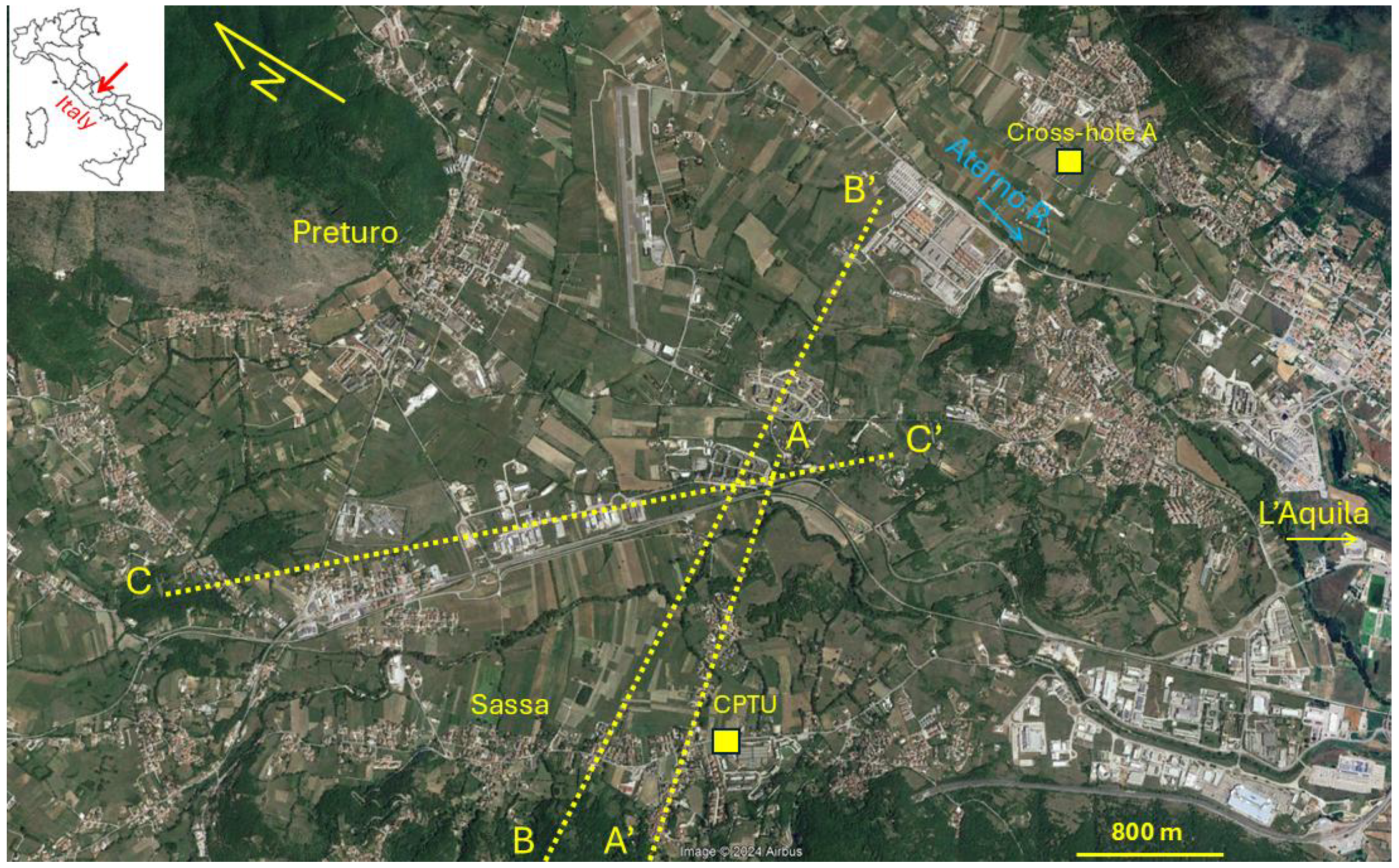
Figure 2.
The study area of Bazzano - Monticchio (eastern districts of L’Aquila Municipality). The yellow lines refer to the sections D-D’ and E-E’ on which numerical simulations were carried out. The Cross-hole B investigation is reported in Section 3.3.
Figure 2.
The study area of Bazzano - Monticchio (eastern districts of L’Aquila Municipality). The yellow lines refer to the sections D-D’ and E-E’ on which numerical simulations were carried out. The Cross-hole B investigation is reported in Section 3.3.
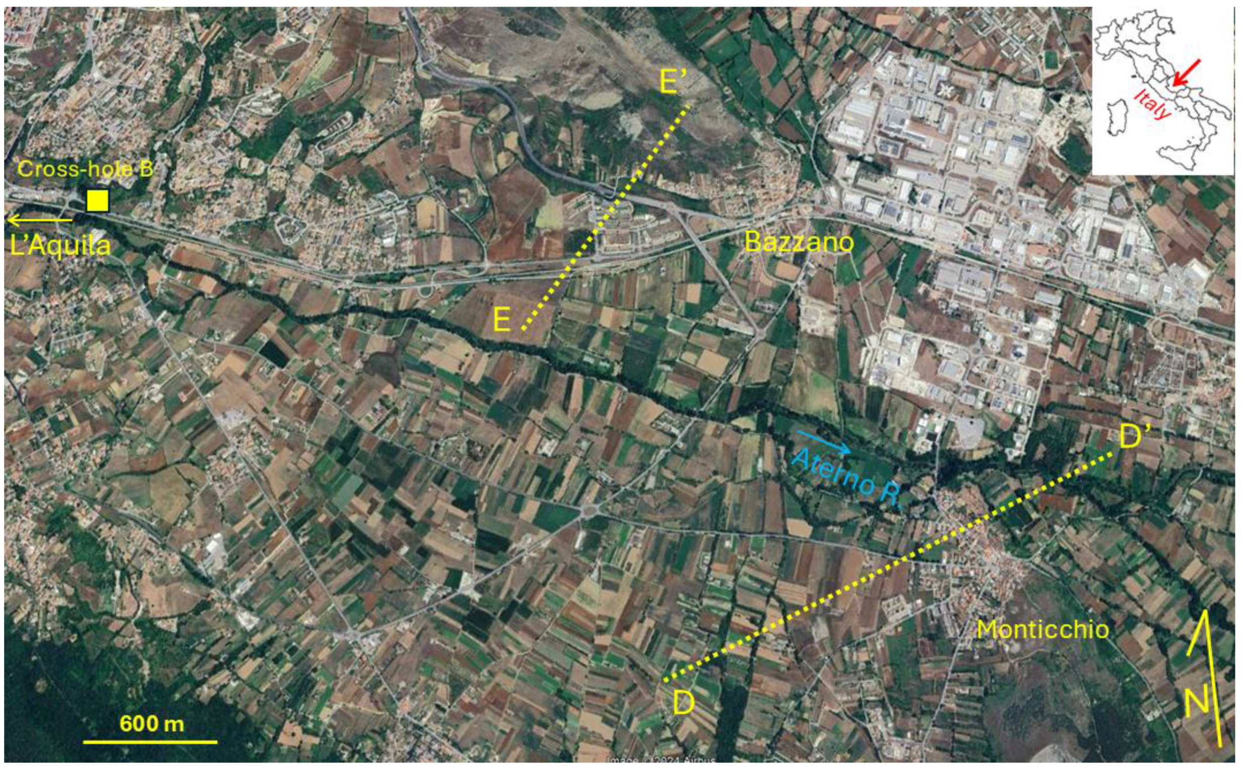
Figure 3.
In the geological sections, representative of the Preturo-Sassa (top) and Bazzano-Monticchio (bottom) areas, the geological relationships of the main units are shown. The Plio-Quaternary L’Aquila basin-cover units are ant, fra, col, at1, all3 S, all3 G, all2, and all1. The units UAP and UAM refer to the terrigenous bedrock; the unit CCD to the carbonate bedrock. For the location of the sections see Figure 1 and Figure 2; for the unit codes and the characteristics of the units see table 1 and 3.
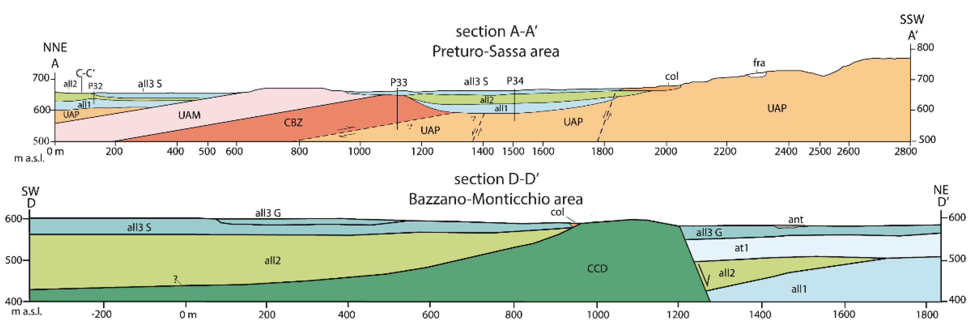
Figure 4.
Investigation map of Sassa pilot area. 1- CPTU; 2- superdeep DCPT; 3- SDMT; 4- down-hole; 5- continuous core borehole; 6- continuous core borehole intercepting the seismic bedrock; 7- trench; 8- microtremor measurement; 9- ERT; 10- MASW; 11- refraction seismics. The blue and red lines refer to the section traces and the boundary of the pilot urban areas studied in the seismic microzonation project. The investigation codes are also reported.
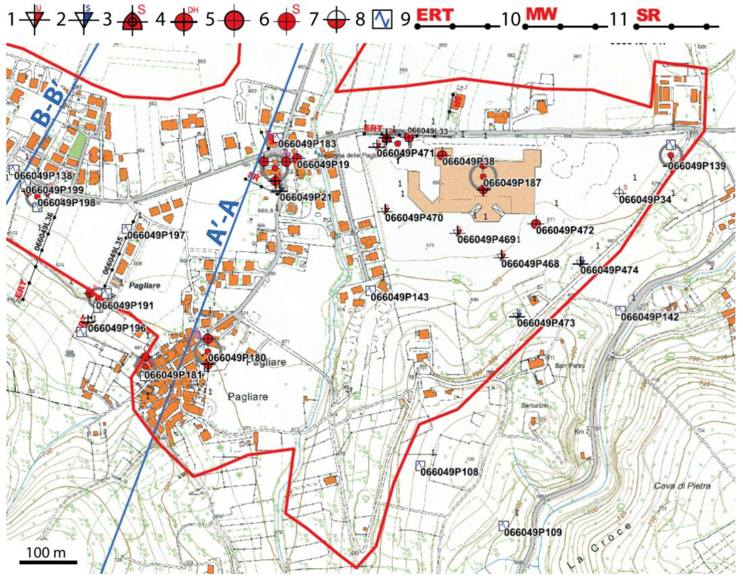
Figure 5.
Resonance frequency map of Sassa pilot area from microtremor measurements. A- amplitude f0 peak; RF: f0 resonance frequency (Hz). The f0 refers to the lowest value of resonance peak in the amplitude versus frequency plot of horizontal to vertical spectral ratio obtained with the microtremor measurement. The blue and red lines refer to the section traces and the boundary of the pilot urban areas studied in the seismic microzonation project. The microtremor measurement codes and the f0 values are also reported.
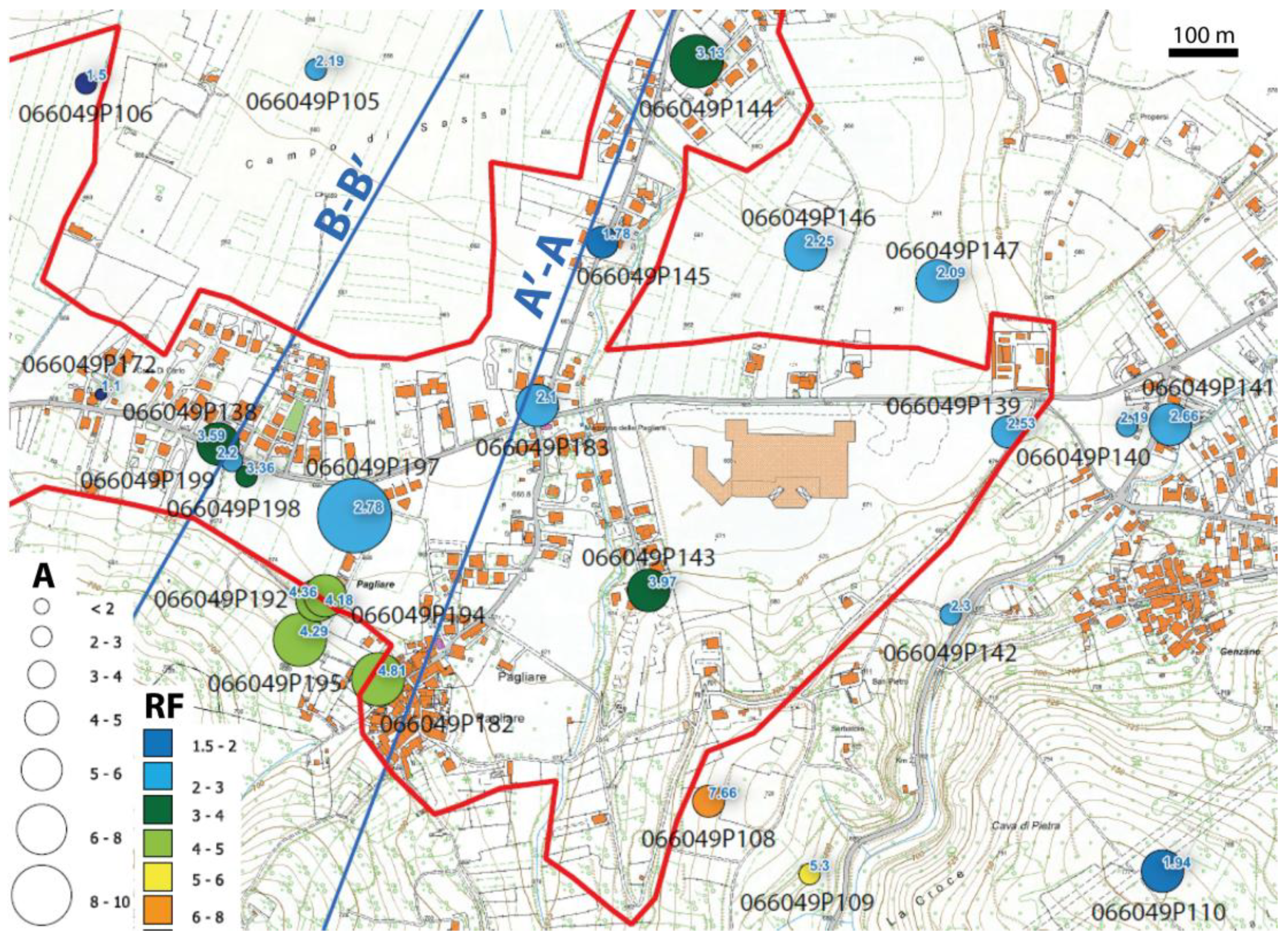
Figure 6.
Representative Vs versus depth investigations. The acronyms refer to the geological units reported in Table 4. The CPTU investigation was acquired into the all3 unit. For the location of the investigation sites see Figure 1 and Figure 2. Cross-hole A and Cross-hole B modified from Del Monaco et al. (2013) and CPTU modified from Chiaradonna et al. (2024).
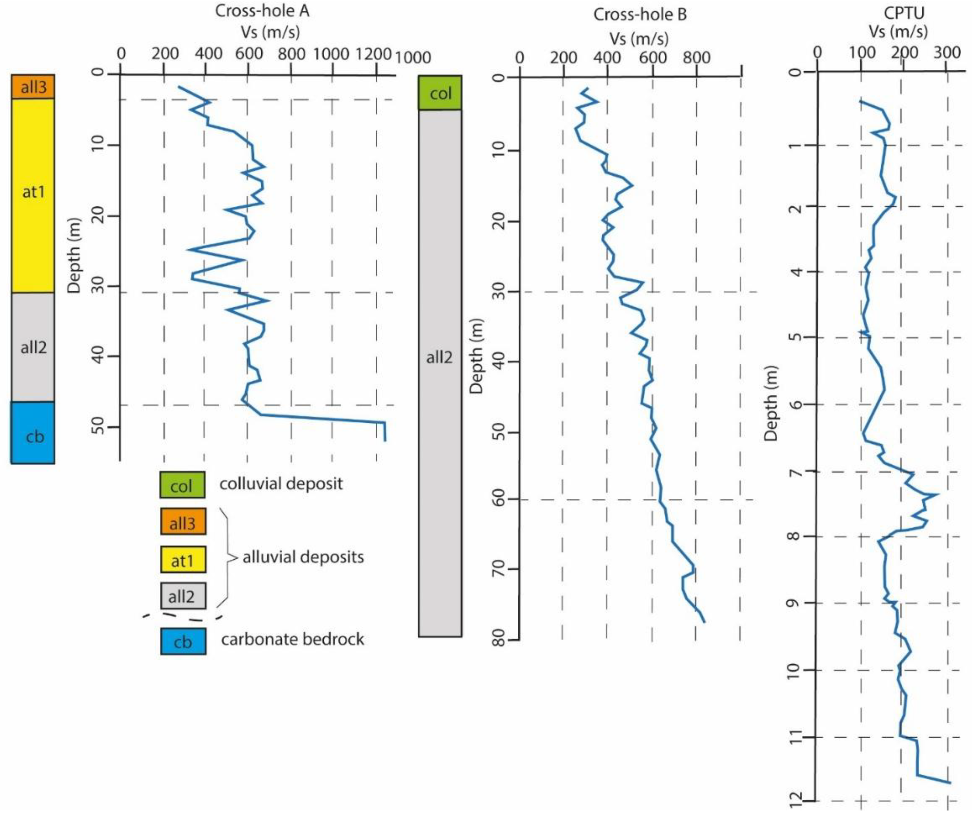
Figure 7.
Spectra of the seven natural accelerograms utilized as input for numerical simulations.
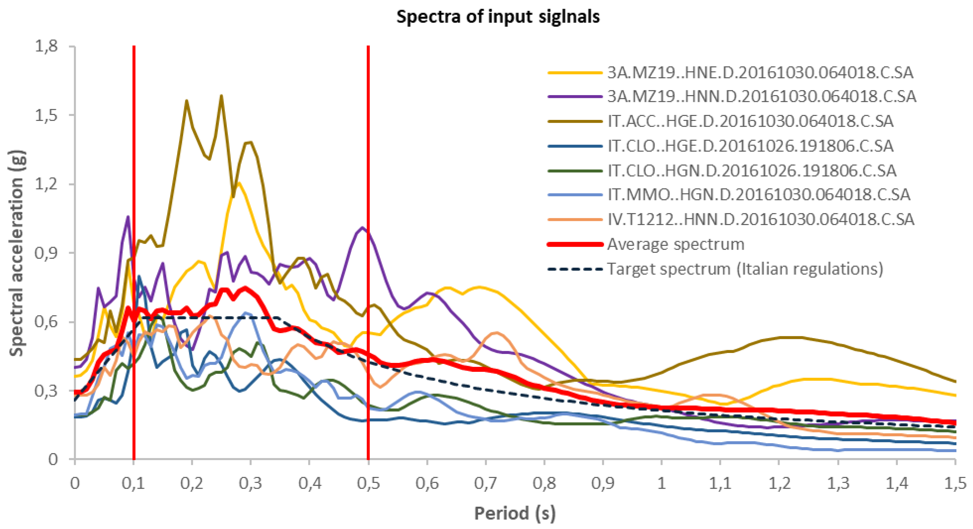
Figure 8.
As an example, the mesh by LSR 2D code is reported (section A-A’; progressive distances: 0-324 m).
Figure 8.
As an example, the mesh by LSR 2D code is reported (section A-A’; progressive distances: 0-324 m).
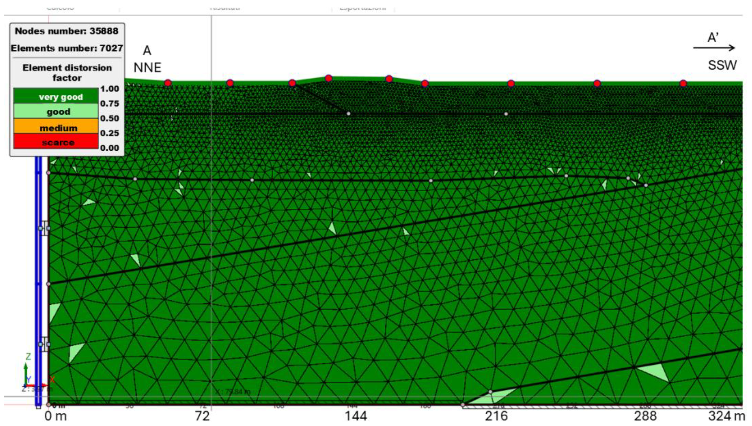
Figure 9.
Section A-A’ (for its location see Figure 1). The unit codes and the geophysical and geotechnical characteristics are reported in table 3. P32-33-34: boreholes. AF intervals: Class 1.0: AF < 1.05; Class 1.7: 1.65 ≤ AF > 1.85; Class 1.9: 1.85 ≤ AF > 2.05; Class 2.1: 2.05 ≤ AF > 2.25; Class 2.3: 2.25 ≤ AF > 2.45.
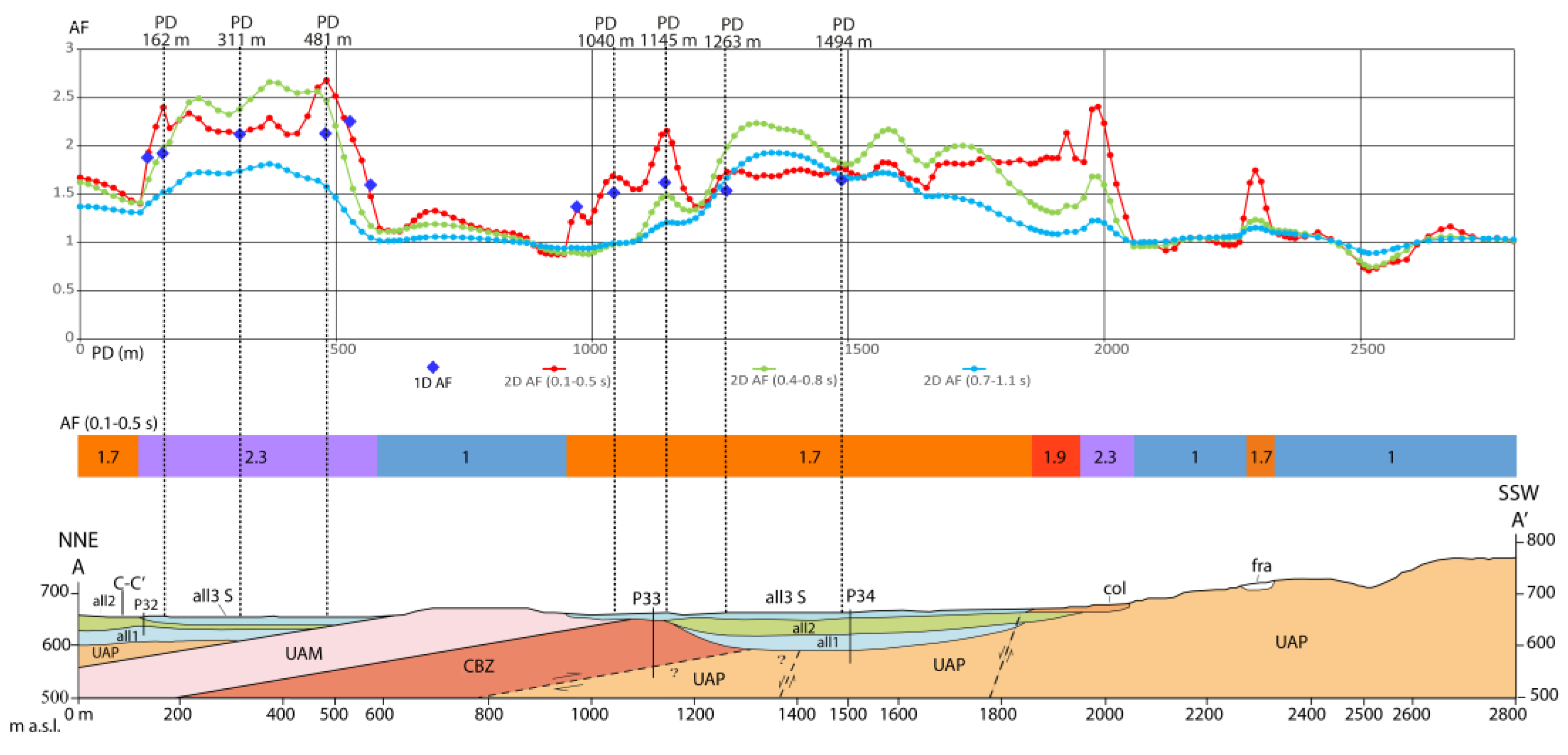
Figure 10.
Part of the section B-B’ (for the location of the whole section trace see Figure 1). The unit codes and the geophysical and geotechnical characteristics are reported in table 3. P20-32-33-34: boreholes. AF intervals: Class 1.5: 1.45 ≤ AF > 1.65; Class 1.7: 1.65 ≤ AF > 1.85; Class 2.3: 2.25 ≤ AF > 2.45.
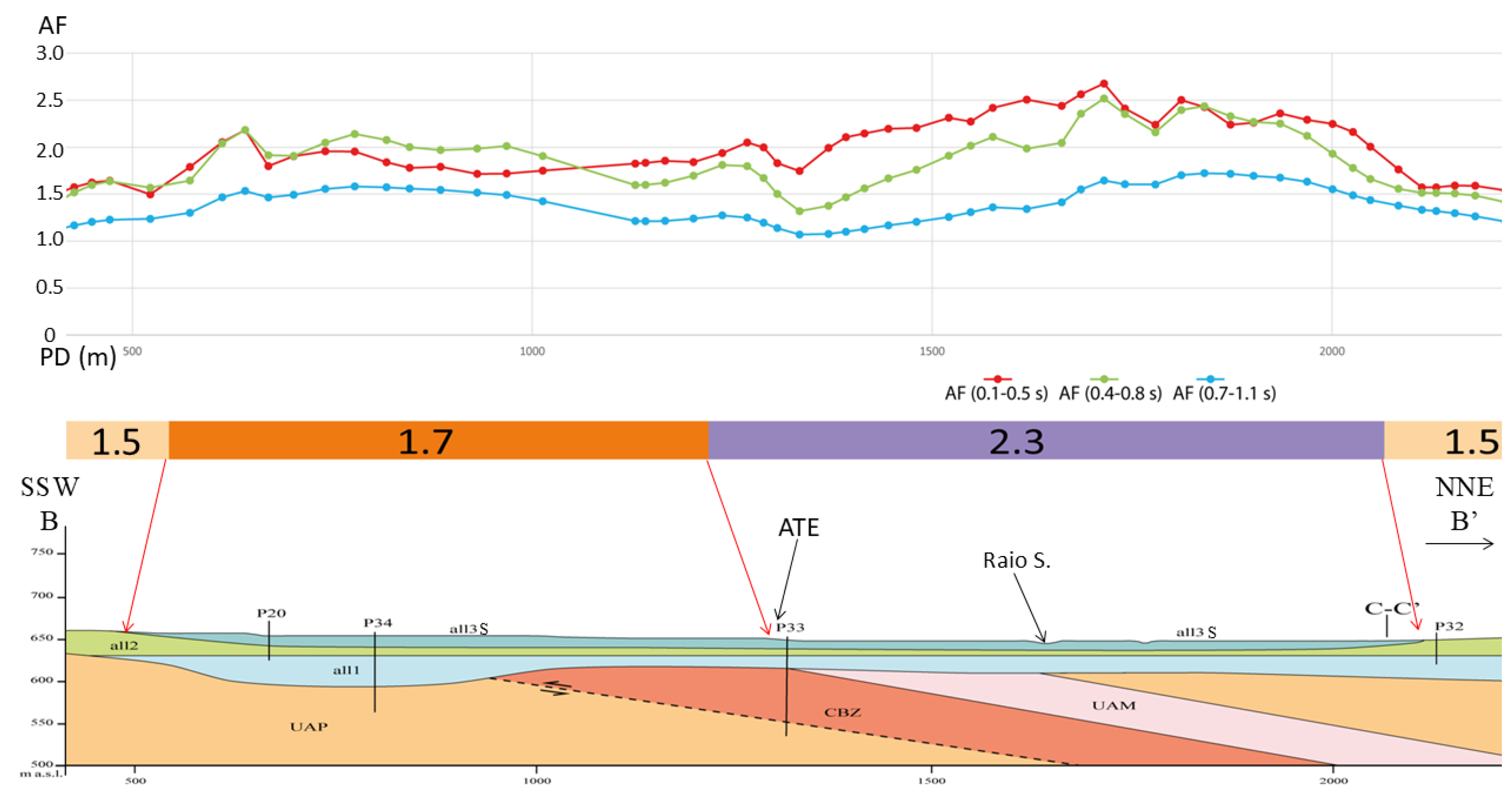
Figure 11.
One-dimensional seismic effect in the wide and shallow basin represented by the section C-C' (for its location see Figure 1) (H/L=70 m/1750 m=0.04, where H is its depth and L is its semi-width). The unit codes and the geophysical and geotechnical characteristics are reported in table 3. AF intervals: Class 1.1: 1.05 ≤ AF > 1.25; Class 1.3: 1.25 ≤ AF > 1.45; Class 1.5: 1.45 ≤ AF > 1.65.
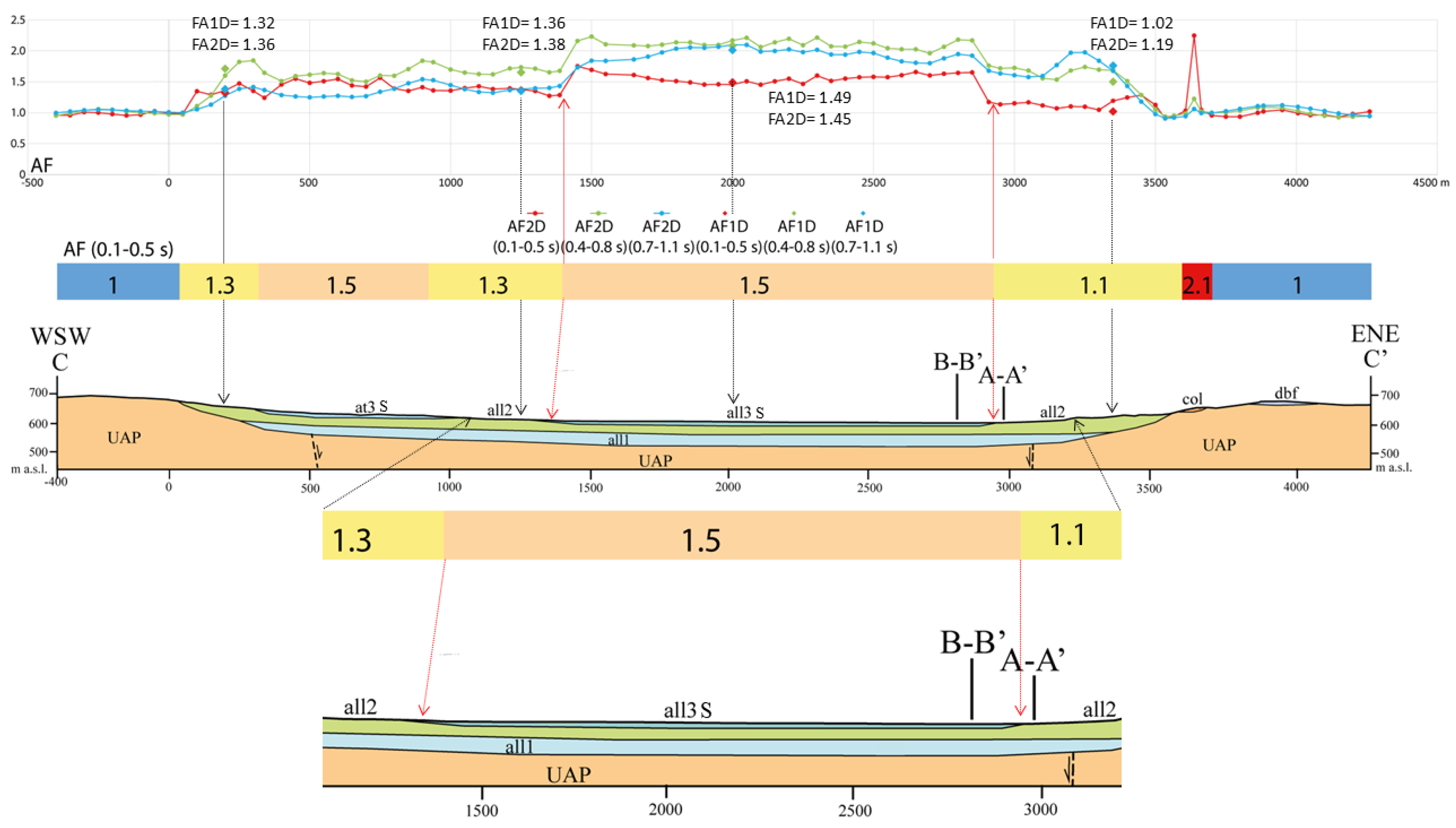
Figure 12.
Section D-D' (for its location see Figure 2); BE: basin edge. The unit codes and the geophysical and geotechnical characteristics are reported in table 3. AF intervals: Class 1.0: AF < 1.05; Class 1.1: 1.05 ≤ AF > 1.25; Class 1.3: 1.25 ≤ AF > 1.45; Class 1.5: 1.45 ≤ AF > 1.65; Class 1.9: 1.85 ≤ AF > 2.05.
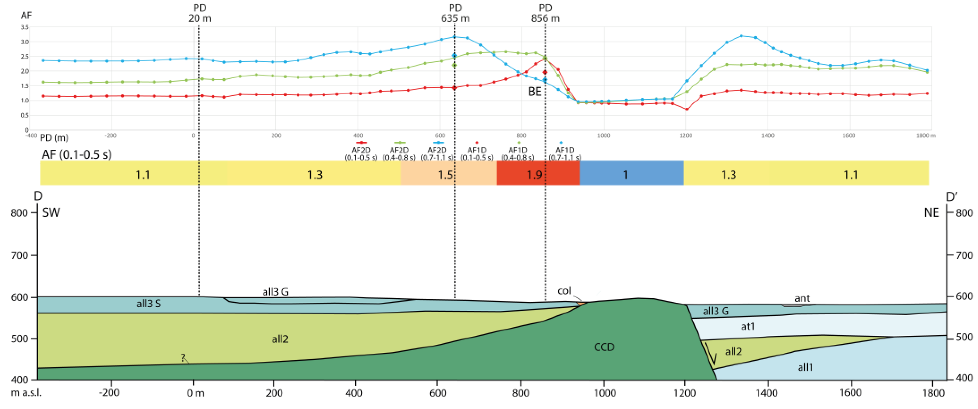
Figure 13.
Section E-E' (for its location see Figure 2); the two arrows show the outcrop area of the terrigenous rocky substratum. P335: borehole. The unit codes and the geophysical and geotechnical characteristics are reported in table 3. AF intervals: Class 1.0: AF < 1.05; Class 1.1: 1.05 ≤ AF > 1.25; Class 1.3: 1.25 ≤ AF > 1.45; Class 1.7: 1.65 ≤ AF > 1.85; Class 1.9: 1.85 ≤ AF > 2.05; Class 2.1: 2.05 ≤ AF > 2.25; Class 2.5: 2.45 ≤ AF > 3.05.
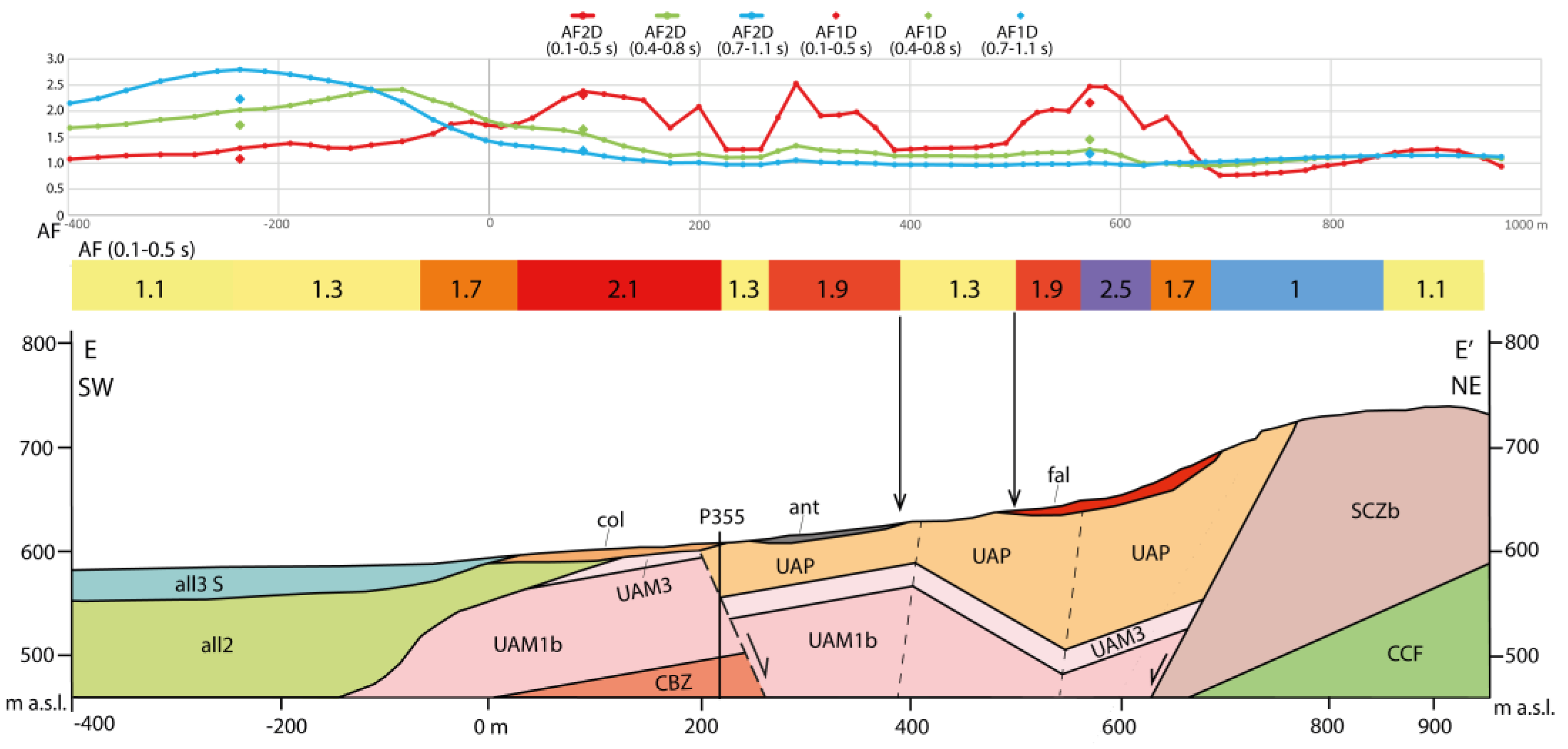
Figure 14.
Comparison of local site response spectra at PD 1040 and PD 1263 in section A’-A reveals distinct features. The AF is estimated by the ratio of the shaded area under the output spectrum to that under the input spectrum. While the spectrum at PD 1040 exhibits a significantly more pronounced peak compared to that at point 1263, the overall areas beneath the two spectra are remarkably similar. Consequently, the calculated amplification factors (AFs) for both points are quite close. The red dotted line denotes the spectrum obtained through the simplified procedure provided by the Italian regulation [CS.LL.PP. 2018].
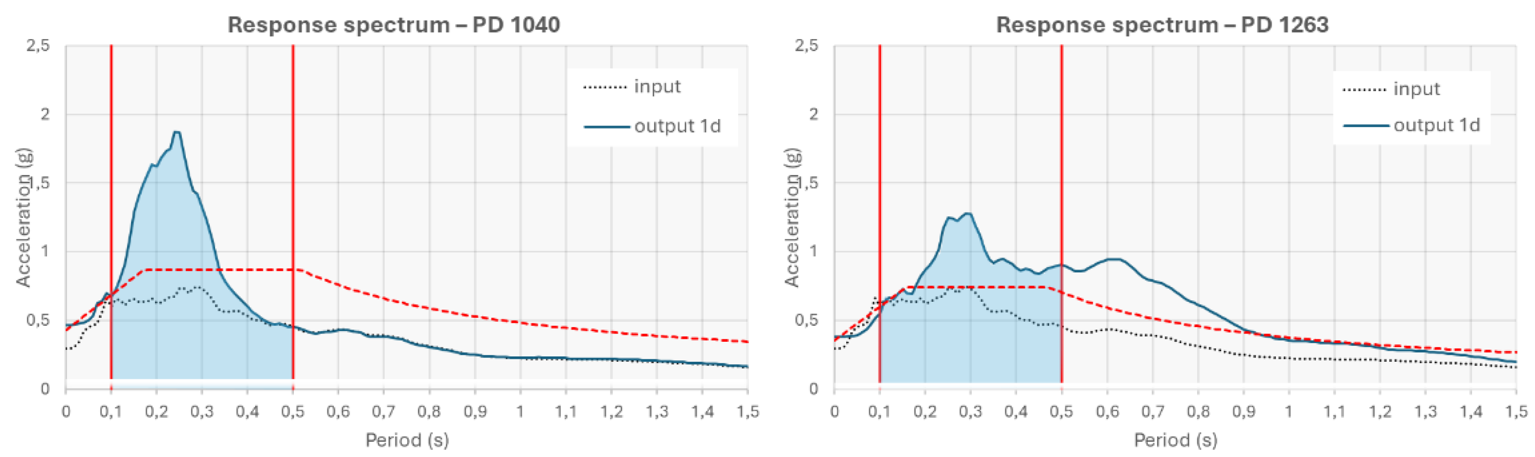
Figure 15.
Response spectra from 1D and 2D simulations in section A’-A at (a) PD 162 m, (b) PD 481 m and (c) PD 1145 m. In these sites 1D and 2D spectra differ as a consequence of 2D site effects. The red dotted line denotes the spectrum obtained through the simplified procedure provided by the Italian regulation [CS.LL.PP. 2018].
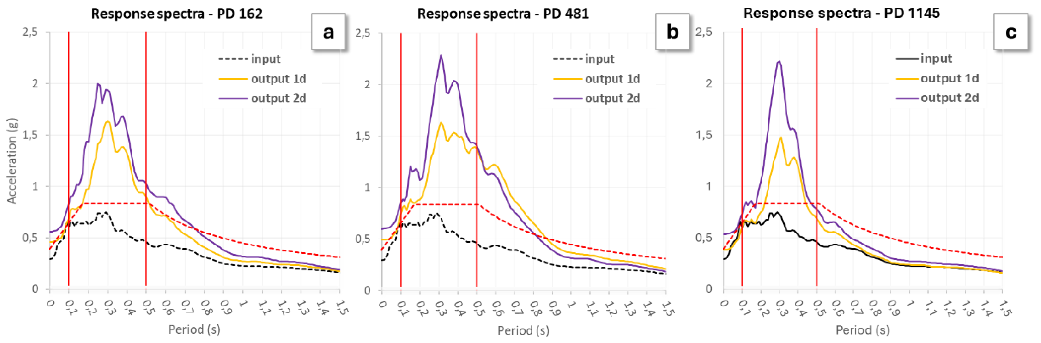
Figure 16.
Response spectra from 1D and 2D simulations in section D-D’ at (a) PD 856 m, (b) PD 635 m and (c) PD 20 m. The occurrence of 2D site effects at PD 856 m is pointed out by the substantial difference between 1D and 2D response spectra, whereas at PD 635 m and 20 m differences are modest or absent. The red dotted line denotes the spectrum obtained through the simplified procedure provided by the Italian regulation [CS.LL.PP. 2018].
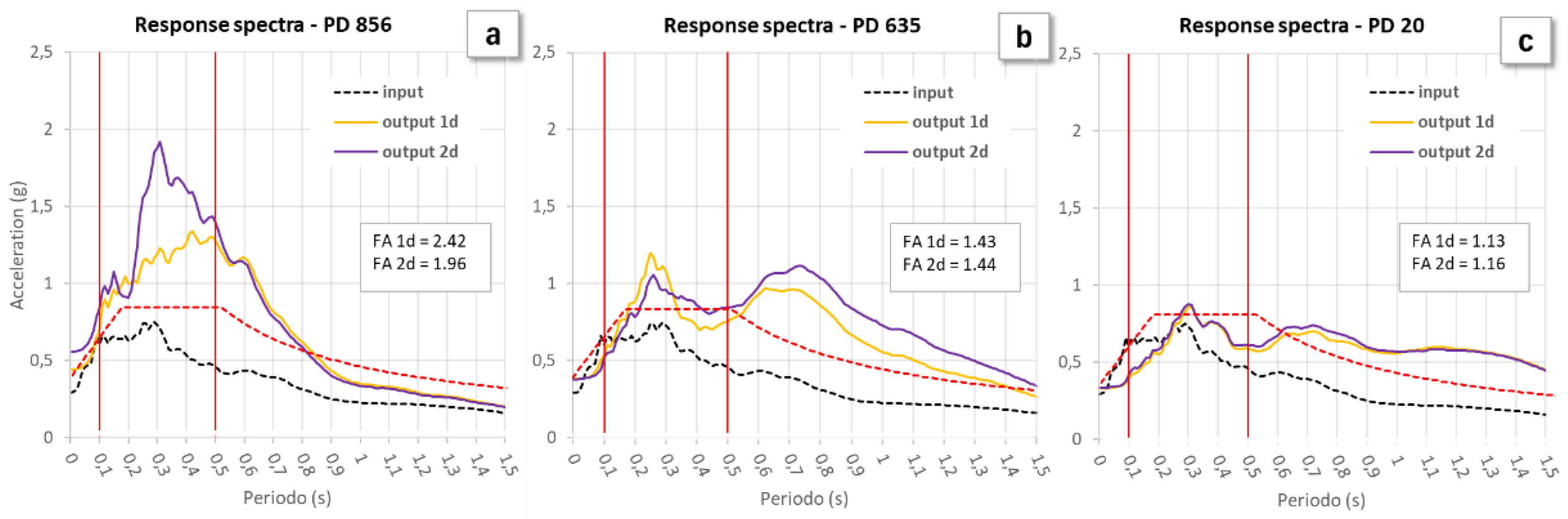
Figure 17.
Comparison between the 1D transfer function obtained for the Progressive Distance 1494 m of section A-A’ (top) and the HVSR plot (bottom) of microtremor measurement acquired near the above-mentioned progressive (066049-P183 in Figure 5). The fair agreement between the resonance frequencies of microtremor and those obtained with the 1D transfer function corroborates the reliability of the subsoil model.
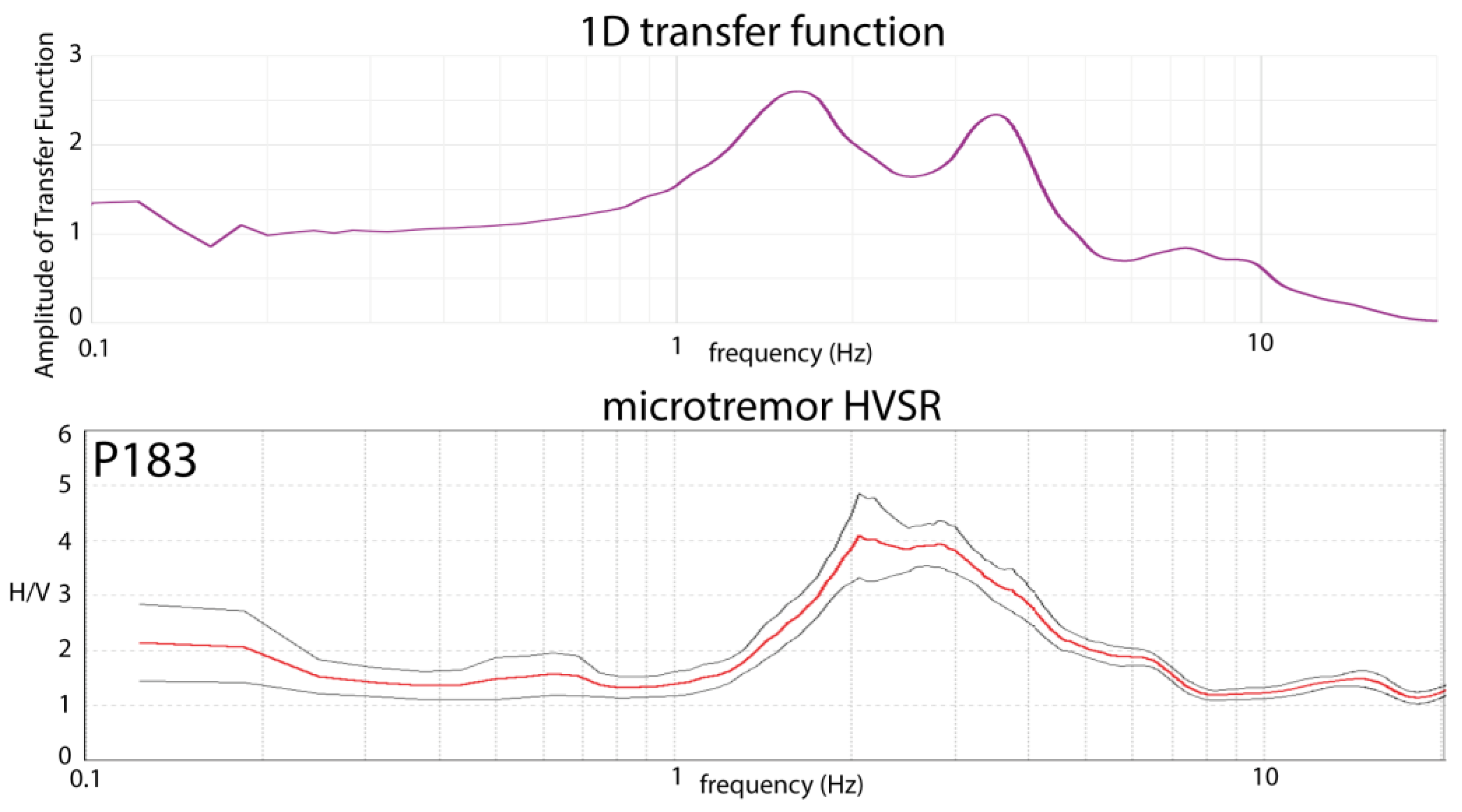

Table 1.
Synthem/Formation and the depositional environment of the L'Aquila Basin units.
| Unit Code (1) | Synthem/Formation (2) | Depositional environment |
|---|---|---|
| ant | - | anthropic deposit |
| fra | Aterno Synthem | landslide deposit |
| fal | Aterno Synthem | slope deposit |
| all3 | Aterno Synthem | fluvial deposit |
| col | Aterno Synthem | Colluvium |
| at3 | Ponte Peschio Synthem | terraced fluvial deposit |
| at2 | Fosso Vetoio Synthem | terraced fluvial deposit |
| dbf | Colle Macchione–L’Aquila Synthem | rock avalanche–debris flow deposit |
| at1 | Fosso Genzano Synthem | terraced fluvial deposit |
| ver | San Marco Formation (Preturo–Sassa area) |
slope deposit San Marco Formation (Preturo–Sassa area) |
| all2 | Madonna della Strada Formation | fluvial deposit |
| all1 | Colle Cantaro-Cave Formation (Preturo–Sassa area) | fluvial deposit (Preturo–Sassa area) |
| all1 | Valle Orsa Formation (Bazzano–Monticchio area) |
fluvial (Gilbert-type fan delta) deposit Valle Orsa Formation (Bazzano–Monticchio area) |
| Ver | Valle Valiano Formation (Bazzano–Monticchio area) |
slope deposit Valle Valiano Formation (Bazzano–Monticchio area) |
| UAP, UAM, UAM3, UAM1b | terrigenous substratum | Upper Miocene siliciclastic foredeep turbidites and hemipelagic pelite |
| CBZ SCZ, and many other codes | carbonate substratum | Mezo-Cenozoic carbonate rocks (ramp, slope-to-basin, and reef environment) |
(1) unit code acronym by Abruzzo Seismic Microzonation Working Group (2012). (2) Plio-Quaternary basin cover units by Nocentini et al. 2017; units of Mezo-Cenozoic substratum by APAT (2006; 2008).
Table 2.
The main investigations and their number of obtained data stored in the QGIS database (total investigations: 527).
Table 2.
The main investigations and their number of obtained data stored in the QGIS database (total investigations: 527).
| Investigation type | Number of obtained data |
| Borehole | 148 |
| dynamic cone penetration test | 13 |
| static cone penetration test | 11 |
| down-hole | 24 |
| MASW | 29 |
| refraction seismics | 5 |
| microtremor measurements | 289 |
| 2D microtremor array | 4 |
| ERT | 4 |
Table 3.
Geophysical and geotechnical characteristics of the units used in all the numerical simulations. The unit weight (kN/m3) of the whole units ranges from 19 to 22 except for anthropic unit (ant) which is 17 kN/m3. The Poisson’s Ratio (ν) of the whole units is 0.2 except for the landslide deposit (fra) and slope deposit (fal) which is 0.4.
| Unit code (+) |
Unit weight (kN/m3) |
Ν | Vs (m/s) |
G/G0 and D versus γ curve |
| Ant | 17 | 0.2 | 250 | gravel (medium) Rollins et al. (1998) |
| Fra | 20 | 0.4 | 300 | gravel (medium) Rollins et al. (1998) |
| Fal | 20 | 0.4 | 300 | gravel (medium) Rollins et al. (1998) |
| all3 S all3 G |
19 | 0.2 | sand (S): 250 gravel (G): 300 |
sand: sand (upper-lower) Seed et al. (1986) gravel: gravel (medium) Rollins et al. (1998) |
| Col | 19 | 0.2 | 250 | sand (upper-lower) Seed et al. (1986) |
| at3 | 19 | 0.2 | 400 | gravel (medium) Rollins et al. (1998) |
| at2 | 19 | 0.2 | 400 | gravel (medium) Rollins et al. (1998) |
| Dbf | 20 | 0.2 | 800 | Modoni and Gazzellone (2010) |
| at1 | 21 | 0.2 | 500 | gravel (medium) Rollins et al. (1998) |
| Ver | 21 | 0.2 | 1200 | elastic linear (damping: 0.5%) |
| all2 (Preturo-Sassa area) | 19 | 0.2 | 450 | sample S3 C3 Cese Preturo (clayey silt) (Working Group MS-AQ, 2010) |
| all2 (Bazzano-Monticchio area) |
19 | 0.2 | 450 (0-30 m) 600 (30-60 m) 700 (60-120 m) 750 (110-160 m) 800 (> 160 m) |
sample S3 C3 Cese Preturo (clayey silt) (Working Group MS-AQ, 2010) |
| all1 | 20 | 0.2 | 800 | gravel (medium) Rollins et al. (1998) |
| terrigenous rocks: UAP, UAM, UAM3, UAM1b | 22 | 0.2 | 800 | elastic linear (damping: 0.5%) |
| carbonate rocks: SCZ, CBZ, etc. | 22 | 0.2 | 1250 | elastic linear (damping: 0.5%) |
unit code acronym by Abruzzo Seismic Microzonation Working Group (2012).
Table 4.
The seven seismic input accelerograms selected by REXELite database (Iervolino et al., 2009) for this study. Seismic network: 3A: Centro di microzonazione sismica Network 2016 Central Italy seismic sequence; IT: Italian Strong Motion Network (RAN) (DPC); IV: Italian National Seismic Network (INGV). Station code: MZ19: Pasciano cemetery – INGV; ACC: Accumoli; CLO: Castelluccio di Norcia; MMO: Montemonaco; T1212: Avendita. The factor scale is 1 for all the selected events. Orientation: the code consists of three alphanumeric characters. The first two characters provide information about the type of sensor and its calibration; the third last letter refers to the recorded direction (N: North; E: East); for all the seven events the horizontal component was selected.
| Seismic network | Station code | Event time | Magnitude (Mw) | Usable bandwidth (Hz) | Orientation | Response spectrum |
|---|---|---|---|---|---|---|
| 3A | MZ19 | 2016-10-30 06:40:18 | 6.5 | 69.96 | HNE |  |
| 3A | MZ19 | 2016-10-30 06:40:18 | 6.5 | 69.96 | HNN |  |
| IT | ACC | 2016-10-30 06:40:18 | 6.5 | 29.94 | HE |  |
| IT | CLO | 2016-10-26 19:18:06 | 5.9 | 39.93 | HE |  |
| IT | CLO | 2016-10-26 19:18:06 | 5.9 | 39.93 | HGN |  |
| IT | MMO | 2016-10-30 06:40:18 | 6.5 | 59.95 | HGN |  |
| IV | T1212 | 2016-10-30 06:40:18 | 6.5 | 49.96 | HNN |  |
Disclaimer/Publisher’s Note: The statements, opinions and data contained in all publications are solely those of the individual author(s) and contributor(s) and not of MDPI and/or the editor(s). MDPI and/or the editor(s) disclaim responsibility for any injury to people or property resulting from any ideas, methods, instructions or products referred to in the content. |
© 2025 by the authors. Licensee MDPI, Basel, Switzerland. This article is an open access article distributed under the terms and conditions of the Creative Commons Attribution (CC BY) license (http://creativecommons.org/licenses/by/4.0/).
Copyright: This open access article is published under a Creative Commons CC BY 4.0 license, which permit the free download, distribution, and reuse, provided that the author and preprint are cited in any reuse.


