
Submitted:
09 May 2025
Posted:
12 May 2025
You are already at the latest version
Abstract
Climate change in recent decades has made exceptional rainfall increasingly frequent, with the consequent risk of flooding of watercourses. Streams and rivers characterized by short flow times are subject to rapid and impressive floods; for this reason, the modeling of their beds is of fundamental importance for the execution of hydraulic calculations capable of predicting the flow rates and identifying the points where floods may occur. In the context of studies conducted on three watercourses in Calabria (Italy), different survey and restitution techniques were used (aerial Lidar, terrestrial laser scanner, GNSS, Photogrammetry). By integrating these methodologies, multi-resolution models were obtained, which constitute the basis of the hydraulic calculations performed. The representations of models and effects that hydraulic calculations have predicted in the event of exceptional rainfall (flow, speed, flooded areas and critical points in the banks) constitute useful tools for designing appropriate defense works and preparing evacuation plans in the event of an alarm, with the aim of mitigating hydrogeological risk.
Keywords:
Geomatics
; Lidar
; Terrestrial Laser Scanner
; Registration
; Modeling Wokflow
; River modeling
; Multiresolution
; 3D models
1. Introduction
According to the definition provided by [1], hydrogeological risk is associated with the natural water cycle and the geological structure of the land. While its primary causes stem from natural factors—such as the country’s climate and geomorphological features—human activities also play a significant role. In recent decades, these anthropogenic influences have increasingly impacted and, in many cases, exacerbated natural processes.
Among the physical factors that predispose the Italian territory (and in particular Calabria) to hydrogeological instability is its geological and geomorphological conformation, characterized by a complex orography and small hydrographic basins, which are therefore characterized by extremely rapid response times to precipitation. Localized and intense meteorological events combined with these characteristics of the territory can therefore give rise to violent phenomena characterized by very rapid kinematics (mudslides and flash floods).
Hydrogeological risk is also strongly influenced by anthropogenic factors. Population density, progressive urbanization, abandonment of mountain lands, illegal building, continuous deforestation, the use of agricultural techniques that do not respect the environment and the lack of maintenance of slopes and watercourses have certainly aggravated the instability and further highlighted the fragility of the Italian territory and increased exposure to such phenomena and therefore the risk itself. [2].
As stated by the Higher Institute for Environmental Protection and Research (ISPRA), 7,423 Italian municipalities—representing 93.9% of the total—are at risk of landslides and floods. Of these 1,701 have their territory classified as areas of medium hydraulic hazard P2, while 4,232 have in their territory both areas at high risk of landslides and medium risk of floods [3].
Bearing in mind the general objective of mitigating hydrogeological risk, watercourse modeling is essential to perform hydraulic calculations that allow forecasting flow rates and identifying points where floods could occur. This information, in fact, can be used to design appropriate defense works and evacuation plans in the event of an alarm.
For several decades, geomatic techniques have been used for the modeling of watercourses, often integrated with each other.
Among these, aerial photogrammetry has long been the main technique [4]. The increasing resolution of digital cameras and the growing computing power of computers, the use of techniques such as Structure from Motion (SfM) [5] have favored the diffusion of this technology for large scale and very large scale mapping, thanks to the possibility of obtaining accurate 3D models even with frames taken by commercial cameras. These techniques are used to study the surface motion of water also in the laboratory [6]. A well-established technique is drone photogrammetry [7]. Thanks to the possibility of orienting the camera through the gimbal system, it is also possible to perform surveys of vertical surfaces, undercuts and intrados of structures.
Significant progress has been made with the use of Light Detection and Ranging (LiDAR) technology, encompassing airborne, terrestrial (TLS), and unmanned aerial vehicle (UAV)-based methods [8].
Airborne LiDAR (ALS) is widely employed for extensive mapping of riverine topography and shallow water. It offers rapid data acquisition over large areas, producing Digital Terrain Models (DTMs) that are valuable for floodplain delineation and geomorphological studies [9]. The possibility of taking acquisitions from above allows the surveying of large surfaces in a short time, but at the same time constitutes a limitation of this technique, especially in correspondence with works of art (bridges). In such circumstances, elements which are fundamental for the execution of hydraulic calculations (like piers, bulkheads, pile caps, abutments) cannot be modelled. It is therefore necessary to carry out surveys of these elements using different techniques and to integrate them.
Terrestrial LiDAR (TLS), including mobile systems such as vehicle-mounted or vessel-mounted mobile systems, offers higher point densities and closer proximity to the riverbed, improving the accuracy of elevation models. This is particularly useful for detailed studies of riverbank morphology and sediment transport processes. Furthermore, the use of TLS allows the acquisition of engineering structures not visible from above [10]. If echosounders are installed on a vessel platform, the survey of bathymetry can be performed.
UAV-based LiDAR, has emerged as a versatile tool for river modeling. Equipped with lightweight LiDAR sensors, UAVs can access challenging terrains and capture high-resolution data with very high point densities [11]. This capability is crucial for mapping intricate features like undercut banks and submerged areas, which are often missed by ALS.
For large areas, the satellite based Synthetic Aperture Radar (SAR) is increasingly used, which allows for the verification of any subsidence phenomena over time [12].
It is almost always necessary to integrate several techniques that allow to obtain complete results thanks to their complementarity [13,14,15]. It is also necessary to consider the need for multi-resolution models, which allow a lower density of points in the areas with a more regular trend and a higher density in the areas where a greater detail is required for the execution of the calculations (for example, in the proximity of artefacts located in the riverbed).
A problem to be addressed is the integration of different geomatics techniques for riverbed surveying, with the aim to combining datasets of different resolutions [16]. In fact, the techniques described above provide complementary data but are inherently heterogeneous in terms of accuracy, scale and spatial density. Discrepancies in resolution often lead to issues such as data misalignment, interpolation artefacts and difficulties in error propagation analysis. In recent years, the integration of multi-source geospatial data has become a central focus in geomatics, particularly in applications involving high-resolution terrain modeling, environmental monitoring, and hydrological analysis.
Among the most effective methods used to face these issues are data fusion techniques, hierarchical surface modeling, and hybrid interpolation schemes. [17,18,19].
A multi-resolution model is obtained by combining multiple models created with different techniques; it is therefore necessary to address the issues related to registration. [20,21]. For this purpose, common points are used, often detected with total stations (TS) or, better, with the use of Global Satellite Navigation Systems (GNSS) receivers that allow georeferencing. As regards referencing, particular attention must be paid to elevations: in fact, orthometric elevations (referred to the geoid) of good precision are necessary for hydraulic calculations to provide reliable results. It is therefore necessary to use the most accurate geoid models available for the area under study [22].
The final output of surveys carried out with geomatic techniques consists of digital terrain model (DTM) and digital elevation model (DEM), which form the basis of hydraulic calculations carried out within a Geographic Information System (GIS) environment or through specialized software [23]. Hydraulic calculations for flood mapping use 1D and 2D modeling. While 2D models provide more accurate and detailed results, they require significantly greater computational resources. However, their use is becoming increasingly common due to advances in computing power [24].
The objective of this article is to present a multi-instrumental approach for hydrogeological hazard assessment, involving the development of heterogeneous models and their integration into a comprehensive multiresolution framework.
The data were acquired as a part of a Regional Operational Programme [25], conducted through a collaborative effort involving three universities and a research center in Italy.
The article is structured as follows: it begins with a description of the surveyed watercourses, the instruments used and techniques employed. This is followed by the presentation of the resulting products and the methods adopted for visualizing the outcomes of the hydraulic computations. The paper concludes with a discussion of the results and the final conclusions.
2. Materials and Methods
2.1. Areas of Study and Their Peculiarities
The study areas are the riverbeds of three watercourses located in the Calabria region, in southern Italy (Figure 1).
2.1.1. Crati River
The Crati river basin has a surface area of 2448.91 km2. With its length of 90 km and the average annual flow of about 36 m³/s, it is the main watercourse of Calabria and the third in southern Italy (Figure 2a). The river has a markedly torrential regime, alternating marked summer low water levels (minimum flow rate approximately 10 m³/s) with strong and sometimes disastrous winter floods (even over 3,000 m³/s). On November 24, 1959, the river flooded, causing extensive damage to homes, shops and department stores (Figure 2b). Characterized by steep slopes and a narrow bed in its first stretch, the river widens at the city of Cosenza, located at the confluence with the Busento river. In this stretch there are several bridges that have been the subject of surveys.
2.1.2. Corace River
The Corace River basin has a surface area of 294.50 km². With a length of 48 km and an average annual flow rate of approximately 4.4 m³/s, the river flows into the Ionian Sea after a course of 48 km (Figure 3a). Also this river has a markedly torrential regime, and several floods happened in the last decades (Figure 3b). In the section between 9 and 10 kilometers from the river mouth, numerous road crossings are present, featuring structures built within the riverbed.
2.1.3. The Fiumara Valanidi
A fiumara is a short watercourse, that remains completely dry for most of the year, due to the scarcity of rainfall. Their bed is very wide and pebbly, with the presence of numerous boulders, evidence of the strong erosive and transport action developed during periods of flooding. The fiumara Valanidi is located south of the city of Reggio Calabria. About 1.5 km from its mouth, it splits into two branches, both characterized by a wide and dry bed, due to the presence of numerous check dams upstream (Figure 4a). The two branches cross the state road E90 that runs along the Ionian Sea. In 1953, after a series of heavy rains, its floods inundated the surrounding area, causing several victims and extensive damage (Figure 4b).
2.2. Instruments Used for Data Acquisition
2.2.1. Aerial Photogrammetry
The aerial photogrammetric survey was performed by helicopter, which allowed the acquisition of shots with a flight height above the ground sufficiently constant even in the areas with a steep slope. The average flight height was 500 meters. The 40 MPixels camera used allowed obtaining orthophotos with a Ground Sampling Distance (GSD) of 20 cm.
2.2.2. Aerial Laser Scanner (ALS)
The ALS survey, realized simultaneously with the photogrammetric shots, was performed with a Riegl LMS-Q680i laser scanner. The point cloud obtained has a density of 4 points/m2. For georeferencing the point clouds, the helicopter was equipped with IMU and GNSS receiver; this equipment ensured an altitude precision of 15 cm.
2.2.3. Terrestrial Laser Scanner (TLS)
To increase the point density near the artifacts present in the riverbed, a RIEGL LMS 420 i vehicle-mounted laser scanner was used. The instrument has a range of 800 m and a precision of 1 cm.
2.2.4. GNSS
Several ground control points (GCP) were surveyed through a Leica Viva GS15 GNSS receiver. The acquisition was performed in rapid-static mode.
2.2.5. Total Station
For the surveying of particular points (vertices on the pier caps, pile caps, etc.), a Leica 1200+ total station was used, with angular precision of 1”, distance precision of +/- 1 mm +/- 1 mm/km and a range without prism of 1200 m.
2.3. Methodologies Adopted for the Integration of Data
To perform hydraulic calculations, a riverbed is represented with a 2.5D model, in which each pair of coordinates in the plan corresponds to a single height. In particular, DTM and DSM are used. The former are used to have the surface of the riverbed without vegetation, while the latter are useful especially in urban areas. The difference between DSM and DTM can provide information on the average height and density of vegetation present, useful for performing hydraulic calculations.
Several authors have proposed 3D modeling workflows that integrate multisensor and multiresolution data, using a combination of methods to produce point clouds and integrated 3D models [26]. In our case we adopted the pipeline represented in Figure 5 for a 2.5D multisensor and multiresolution modeling, based on the integration of different techniques, aimed at generating riverbed models.
As for the laser scanner data, typical procedures for processing point clouds were used. After eliminating outliers and thinning out excessively dense areas, hole filling was performed. In the case of river surveys, this operation is particularly delicate: the holes in the meshes obtained, generally caused by undercuts or the presence of elements that hide the undetected areas, are often due to the presence of water. Filling the holes, in this case, would lead to the creation of incorrect models, which would distort the results of hydraulic calculations.
The coarse georeferencing of the aerial surveying was obtained through IMU and GNSS receiver operating in kinematic mode. The acquisitions of the Continuously Operating Reference Stations (CORS) present in the surroundings of the three surveyed areas have been used. Subsequently, GCPs surveyed on the ground by GNSS or Total Station receivers were used.
The terrain model obtained from the aerial laser scanner was then appropriately verified. The point clouds acquired in adjacent strips have overlapping areas. To evaluate the accuracy of their alignment, after selecting the common area, the deviation between the overlapping meshes is calculated. Based on the trend of the deviations, the registration can be refined.
The possibility of discriminating the first and the last pulse was exploited. This opportunity allowed to obtain both the DSM and the DTM of the surveyed areas (Figure 6). The DTM is used for hydraulic calculations in the riverbed area, but the DSM plays a fundamental role, especially in urbanized areas, to be able to predict the effects of a flood. The difference between DSM and DTM, i.e. the difference between the first and the last pulse, can provide, in the riverbed areas, the average height of the vegetation and its density, which allow an accurate evaluation of the roughness.
The georeferencing of the land survey was obtained through a GNSS receiver operating in rapid-static mode. Also in this case, the acquisitions of the CORS present in the surrounding environment were used. The GCP points were surveyed and several tie points were selected. The GCPs were identified in order to serve for the georeferencing of the acquisitions. They coincide with fixed elements (vertices of bridge railings, riverbank parapets, road signs, etc.) easily identifiable in the point clouds obtained from aerial and terrestrial shots (Figure 7). Some points were identified inside the riverbeds or at the natural riverbanks, essentially on boulders or tree trunks present (Figure 8); these were used only for the georeferencing the point clouds acquired by the TLS, as the survey with ALS had been performed on a different date.
As regards the heights, the Quasi-Geoid ITALGEO05 was used, which covers the Italian territory [22].
The registration of the point clouds obtained from ALS and TLS was obtained by exploiting the GCPs and common features. Common surfaces—specifically horizontal and sub-vertical ones—were utilized during the process. Vertical surfaces help refine horizontal alignment, whereas horizontal surfaces are used to improve vertical registration (Figure 9). This last operation is particularly important, given that the points’ elevations play a fundamental role in hydraulic calculations. The orthometric heights of the models obtained by TLS were chosen as reference.
2.4. Integration of Datasets for Hydrological Modeling
From the point clouds acquired with the ALS for each river, a Triangulated Irregular Network (TIN) was obtained. To reduce computational load during hydrological simulations, a simplification step was applied to the TIN in relatively flat or homogeneous regions. A decimation algorithm, available in open-source tools [27], was used in these regular areas; this retained detail in complex terrain while significantly reducing the number of elements in the mesh. As for points acquired with TLS, the decimation is essential. While the points acquired with ALS are uniformly distributed (in our case 4 points/m2), in the case of TLS there is an excessive density in proximity to the instrument, which must be eliminated in order not to have an excessive calculation effort without having as a counterpart useful information for hydraulic calculations.
To construct a continuous and hydrologically accurate terrain model, we integrated the Triangulated Irregular Network (TIN) datasets acquired by ALS and TLS representing adjacent or overlapping regions of the study area. The integration aimed to eliminate discontinuities or mismatches that could adversely affect hydrological simulations such as flow routing or watershed delineation.
After preprocessing and registration, the procedure involved the following steps:
- -
- Shared edges and overlapping zones were identified. Duplicate or closely spaced vertices within these areas were removed or averaged, and edge snapping was applied to ensure seamless connectivity.
- -
- The merged point set was re-triangulated to form a new TIN structure using Delaunay triangulation. Special attention was given to preserving terrain features and ensuring topological correctness, particularly in areas critical for water flow such as ridges and depressions.
3. Results
3.1. Orthophoto
Orthophotos are a first product, easily obtainable through ALS acquisitions combined with aerial imagery. In our case they were used not only as documentation, but also to identify those structures designated as housing or production activities that insist on flood areas. This information is useful to determine exposure and vulnerability and, consequently, risk, i.e. the potential impact of a hazard, (Risk = Hazard x Exposure x Vulnerability). In our case the hazard is a flood with a return period of 200 or 500 years. In Figure 10, the production and residential settlements in the central stretch of the fiumara Valanidi are visible.
3.2. Meshing of ALS and TLS Point Clouds
The union of point clouds acquired from ALS and from TLS offers the possibility of exploring the area of interest for hydraulic calculations. It is an aid in identifying singularities (artifacts, abrupt variations in slope of the ground bed, etc.) in proximity of which it is necessary to refine the TIN.
Figure 11 shows a central section of the Corace River. TLS-acquired points are shown in green, while ALS-acquired points are displayed in blue. In panel (a), some retaining walls which surface was used for registration are highlighted with red ellipsles. The bridge deck shown in Figure 9, used for vertical alignment during registration, is highlighted in yellow. In both panels of the figure, the different density of the point clouds acquired by ALS and TLS is evident.
3.3. Multiresolution TIN
One of the most significant results obtained is the variable-resolution TIN, which was used for hydraulic calculations [24]. Figure 12 illustrates a section of the Corace River featuring a bridge (panel a); the TIN generated from ALS data, with 3D models of the bridge plinths and piers overlaid, derived from TLS and Total Station data (panel b); and the mesh refinement applied in the central area of the bridge (panel c).
3.4. 2.5D Views per Rappresentazione dei Risultati
These views are particularly useful for visualizing and interpreting the results of hydraulic calculations—such as water depth, flow velocity, and flood extent—as they enhance the understanding of spatial patterns and flow behavior. In this study, the visualizations were generated using the software ER Mapper ® [29]. Several thematic layers were represented, each illustrating different aspects of the hydraulic modeling results, including flow velocity, eta, and sediment deposition.
Figure 13 (a) displays the 2.5D model of the fiumara Valanidi, illustrating water velocity during a 500-year return period flood event. Velocity values are represented using a color scale, increasing from violet to red. Several flooding points are visible along the river corridor. Panel (b) provides a zoomed-in view of the central area; on the hydraulic left, a critical point is highlighted where the riverbanks are insufficient to contain the flow, resulting in overtopping and local flooding.
3.5. Representation of Results on the Regional Technical Map
Regarding the 2D maps, these were produced to visualize the modeling results over the base cartography of the study area. Figure 14 shows the Eta thematic layer displayed on a 1:5,000 scale technical map.
3.6. Representation on Orthophotos with Enhanced Detail
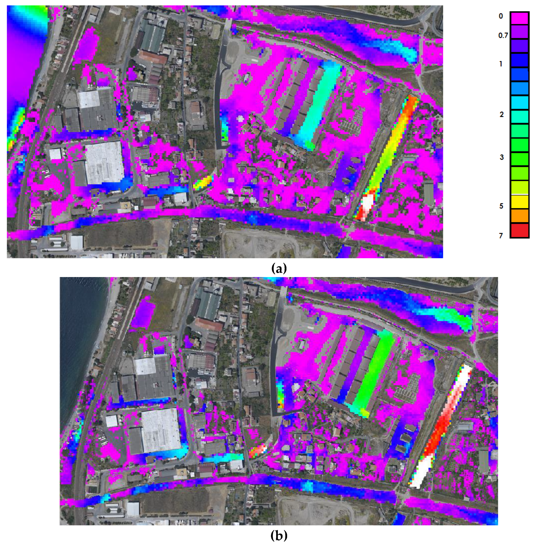
The final output consists of representing the thematic data on an orthophoto. This was initially achieved using an image with a Ground Sampling Distance (GSD) matching the resolution of the hydraulic model’s calculation grid. Specifically, Figure 15(a) illustrates the deposition theme overlaid on an orthophoto with a pixel size of 5 × 5 meters.
To enhance the detail of the representation, a higher-resolution orthophoto with a GSD of 1 meter was used. Although the hydraulic calculations were performed on a 5 × 5 m grid, the finer 1 × 1 m cells—corresponding to image pixels—were introduced purely for visualization purposes. The deposition values within each 5 × 5 m cell were redistributed over the 25 corresponding 1 × 1 m image pixels using the following equation:
where:
Di = D + (hm – hi)
D is the deposition value in the 5 x 5 m cell
Di is the deposition value in the ith 1 x 1 m cell
hm is the orthometric height of the 5 x 5 m cell
hi is the orthometric height of the 1 x 1 m cell
This method provides a smoother and more detailed visual representation, without altering the resolution of the original hydraulic computations. Negative values of Di are set to zero:
IF Di < 0 then Di=0
A further refinement was then performed, to account for the residual deposition R, calculated as follows:
This residual represents the difference between the total deposition assigned to the original 5 × 5 m cell and the sum of the interpolated values distributed among the 25 corresponding 1 × 1 m pixels. To preserve mass balance, the residual R was redistributed equally among the pixels where Di ≥ 0. Let n be the number of such pixels. A second approximation of the deposition value, Di,2, was then computed as:
IF Di≥0 then Di,2 = Di + R/n
Due to the relatively small magnitude of R/n, no further iterative corrections were considered necessary.
The procedure described above enabled a more realistic representation, in which features such as building walls, retaining structures, and artificial embankments are clearly highlighted. The benefits of this refined visualization go beyond aesthetics: the increased level of detail improves the identification of man-made elements within potentially flooded areas. In some cases, the enhanced resolution also makes it possible to reassess results initially derived using coarser calculation cells, potentially leading to significantly different values and highlighting the need for more refined hydraulic calculation. This is clearly illustrated in Figure 15B, where the artifacts are not only more distinctly highlighted, but also significant variations in the thematic values are evident. In particular, on the right side of the figure, the deposition values are noticeably higher in the trench area of the E90 road, located between the two final branches of the fiumara.
4. Discussion
In the context of hydrogeological risk mitigation, the integration of ALS and TLS point clouds represents a key step toward developing accurate and actionable terrain models. The successful meshing of these datasets relies heavily on robust registration techniques. In this case, a multi-instrumental approach was adopted, which is reflected in the integrated use of various point cloud registration techniques. These included the use of ground control points (GCPs), alignment based on sub-vertical and horizontal surfaces, and subsequent refinement through the Iterative Closest Point (ICP) algorithm. The peculiarity of the presented application lies in both its spatial extent—comprising two segments of approximately 10 km and one of 40 km—and in the diverse nature of the watercourses analyzed, ranging from a typical river to fiumara-type torrents.
The multi-instrumental approach also supported the targeted identification of areas to be modeled using TINs with varying levels of resolution. The final multiresolution TIN offers several advantages. It supports the detection of small-scale features—such as incipient erosion, structural discontinuities, or sediment accumulation zones—that may be overlooked in uniform-resolution models. Furthermore, the enhanced detail in high-risk zones allows for more accurate hydraulic simulations, which are essential for assessing flood paths, sediment dynamics, and the impact of protective infrastructure.
A particular methodology has been introduced to refine the representation of the “deposit” theme, moving from the resolution of the hydraulic calculation to that of the orthophotos. The refined orthophoto serves as a valuable tool in the broader effort to mitigate hydrogeological risk. By integrating thematic data—such as deposition values—into a high-resolution, georeferenced image, it becomes possible to more effectively visualize not only the spatial distribution of key parameters but also the interaction between natural processes and human-made features. The ability to identify structures such as check dams, embankments, road trenches, and retaining walls directly from the orthophoto enhances the interpretation of hydraulic modeling results. Specifically, the enhanced resolution enables the precise delimitation of vulnerable zones and existing infrastructure. From a planning and decision-making perspective, such a product supports more informed risk assessments. It enables civil protection authorities and engineers to better locate intervention priorities, calibrate hydraulic models more accurately, and even reconsider the placement or effectiveness of structural mitigation measures. Therefore, the orthophoto is not merely a background image, but an analytical tool that bridges hydraulic modeling and territorial planning, helping to translate technical results into practical actions aimed at reducing hydrogeological hazards.
Author Contributions
Conceptualization, S.A. and G.A.; methodology, S.A.; validation, S.A. and G.A.; formal analysis, G.A.; investigation, S.A.; data curation, S.A.; writing—original draft preparation, S.A.; writing—review and editing, S.A. and G.A.; visualization, S.A.; supervision, S.A.. All authors have read and agreed to the published version of the manuscript.
Funding
This work was supported in part by the European Union and the Region of Calabria in the funding project POR Calabria 2000–2006 Asse 1, Misura 1.4, Azione 1.4.c, ‘‘Studio e sperimentazione di metodologie e tecniche per la mitigazione del rischio idroge-ologico’’ Lotto 8 ‘‘Metodologie di individuazione delle aree soggette a rischio idraulico di esondazione” (scientific responsible prof. Francesco Macchione).
Data Availability Statement
The original contributions presented in this study are included in the article. Further inquiries can be directed to the corresponding author.
Conflicts of Interest
The authors declare no conflicts of interest.
References
- Civil Protection Department of Italy: on the right side of the figure. Available online: https://www.protezionecivile.gov.it/it/approfondimento/descrizione-del-rischio-meteo-idrogeologico-e-idraulico/ (accessed on 15-4-2025).
- Presidency of the Council of Ministers Italian Civil Protection Department: National risk assessment Overview of the potential major disasters in Italy: seismic, volcanic, tsunami, hydro-geological/hydraulic and extreme weather, droughts and forest fire risks updated: December 2018. Available on line: https://www.protezionecivile.gov.it/static/ 5cffeb32c9803b0bddce533947555cf1/ Documento_sulla_Valutazione_nazionale_dei_rischi.pdf (accessed on 15/04/2025).
- Higher Institute for Environmental Protection and Research (ISPRA) Hydrogeological instability in Italy: hazard and risk indicators 2021 Edition. ISPRA Reports 356/2021. Available on line: https://www.isprambiente.gov.it/files2022/pubblicazioni/rapporti/rapporto_dissesto_idrogeologico_italia_ispra_356_2021_finale_web.pdf (accessed on 15/04/2025).
- Pleterski, Ž.; Hočevar, M.; Bizjan, B.; Kolbl Repinc, S.; Rak, G. Measurements of Complex Free Water Surface Topography Using a Photogrammetric Method. Remote Sens. 2023, 15, 4774. [CrossRef]
- Javernick, L.; Brasington, J.; Caruso, B. Modeling the topography of shallow braided rivers using Structure-from-Motion photogrammetry. Geomorphology 2014, 213, 166–182.
- Artese S, Perrelli M, Tripepi G, Aristodemo F. Dynamic measurement of water waves in a wave channel based on low-cost photogrammetry: description of the system and first results. In: R3 in Geomatics: Research, Results and Review; Parente, C., Troisi, S., Vettore, A. Eds.; Springer Nature, Berlin, Germany, 2019, Vol. 1246, p. 198.
- Szostak, R.; Pietroń, M.; Wachniew, P.; Zimnoch, M.; Ćwiąkała, P. Estimation of Small-Stream Water Surface Elevation Using UAV Photogrammetry and Deep Learning. Remote Sens. 2024, 16, 1458. [CrossRef]
- Hohenthal, J., Alho, P., Hyyppä, J., & Hyyppä, H. Laser scanning applications in fluvial studies. Progress in Physical Geography 2011 35(6), 782-809. [CrossRef]
- Mandlburger, G., Pfennigbauer, M., Schwarz, R., and Pöppl, F. A decade of progress in topo-bathymetric laser scanning exemplified by the pielach river dataset. ISPRS Ann. Photogramm. Remote Sens. Spatial Inf. Sci. 2023, X-1/W1-2023, 1123–1130. [CrossRef]
- Artese S. The Survey of the San Francesco Bridge by Santiago Calatrava in Cosenza, Italy. ISPRS-International Archives of the Photogrammetry, Remote Sensing and Spatial Information Sciences. 2019, XLII-2/W9, 33-37.
- Barbero-García, I.; Guerrero-Sevilla, D.; Sánchez-Jiménez, D.; Marqués-Mateu, Á.; González-Aguilera, D. Aerial-Drone-Based Tool for Assessing Flood Risk Areas Due to Woody Debris Along River Basins. Drones 2025, 9, 191. [CrossRef]
- Artese G., Fiaschi S., Di Martire D., Tessitore S., Fabris M., Achilli V., Ahmed A., Borgstrom S., Calcaterra D., Ramondini M., Artese S., Floris M., Menin A., Monego M., Siniscalchi V. Monitoring of Land Subsidence in Ravenna Municipality Using Integrated SAR-GPS Techniques: Description and First Results. ISPRS - International Archives of the Photogrammetry, Remote Sensing and Spatial Information Sciences 2016, XLI-B7, 2016, pp.23-28, DOI 10.5194/isprs-archives-XLI-B7-23-2016.
- Backes, D., Smigaj, M., Schimka, M., Zahs, V., Grznárová, A., and Scaioni, M. River morphology monitoring of a small-scale alpine riverbed using drone photogrammetry and lidar. Int. Arch. Photogramm. Remote Sens. Spatial Inf. Sci. 2020, XLIII-B2-2020, 1017–1024. [CrossRef]
- Kotlarz, P., Siejka, M., & Mika, M. Assessment of the accuracy of DTM river bed model using classical surveying measurement and LiDAR: a case study in Poland. Survey Review 2019, 52(372), 246–252. [CrossRef]
- Artese, S., Perrelli, M., Rizzuti, F., Artese, F., Artese, G. The integration of a new sensor and geomatic techniques for monitoring the Roman bridge S. Angelo on the Savuto river (Scigliano, Italy). International Conference on Metrology for Archaeology and Cultural Heritage, IMEKO, Budapest, Hungary, 2022, pp. 191–195.
- Abrahart, R., See, L. M. Multi-model data fusion for river flow forecasting: An evaluation of six alternative methods based on two contrasting catchments Hydrology and Earth System Sciences 2002, 6(4). [CrossRef]
- Brodu, N., & Lague, D. 3D terrestrial lidar data classification of complex natural scenes using a multi-scale dimensionality criterion: Applications in geomorphology. ISPRS Journal of Photogrammetry and Remote Sensing 2012, 68, 121–134.
- Uciechowska-Grakowicz, A.; Herrera-Granados, O. Riverbed Mapping with the Usage of Deterministic and Geo-Statistical Interpolation Methods: The Odra River Case Study. Remote Sens. 2021, 13, 4236. [CrossRef]
- Passalacqua, P., Belmont, P., & Foufoula-Georgiou, E. Automatic geomorphic feature extraction from lidar in flat and engineered landscapes. Water Resources Research 2015, 51(3), 1794–1821.
- Pirotti, F., Guarnieri, A., Chiodini, S., and Bettanini, C. Automatic coarse co-registration of point clouds from diverse scan geometries: a test of detectors and descriptors, ISPRS Ann. Photogramm. Remote Sens. Spatial Inf. Sci. 2023, X-1/W1-2023, 581–587. [CrossRef]
- Xu, N., Qin, R., Song, S. Point cloud registration for LiDAR and photogrammetric data: A critical synthesis and performance analysis on classic and deep learning algorithms, ISPRS Open Journal of Photogrammetry and Remote Sensing 2023, Volume 8, 2023, 100032. [CrossRef]
- Barzaghi, R., Borghi, A., Carrion, D., Sona, G. Refining the estimate of the Italian quasi-geoid, Bollettino di Geodesia e Scienze affini 2007, 3, 145-160.
- Artiglieri, P., Curulli, G., Coscarella, F., Algieri Ferraro, D., Macchione, F. Performance of HEC-RAS v6.5 at basin scale for calculating the flow hydrograph: comparison with TUFLOW. Natural Hazards 2025, 121-3. [CrossRef]
- Costabile, P., Macchione, F., Natale, L., Petaccia, G. Flood mapping using LIDAR DEM. Limitations of the 1-D modeling highlighted by the 2-D approach. Nat Hazards 2015, 77, 181–204. [CrossRef]
- Macchione, F. (Scientific coordinator). Final reports of the POR Calabria 2000–2006 project “Methods for the Identification of Areas at Hydraulic Flood Risk” 2012, conducted in collaboration with CUDAM (University of Trento), the University of Pavia, and the National Institute of Oceanography and Experimental Geophysics – OGS (Trieste).
- Remondino, F., Rizzi, A. Reality-based 3D documentation of natural and cultural heritage sites—techniques, problems, and examples. Appl Geomat 2010, 2(3), 85–100, DOI 10.1007/s12518-010-0025-x.
- MeshLab. Available online: https://www.meshlab.net/ accessed on 10-02-2023.
- QGIS. Available online: https://qgis.org/ accessed on 10-02-2023.
- ER Mapper manual. Available online: https://www.planetek.it/media/download/er_mapper accessed on 10-02-2023.
Figure 1.
Southern Italy - the basins of the studied watercourses are circled in yellow.
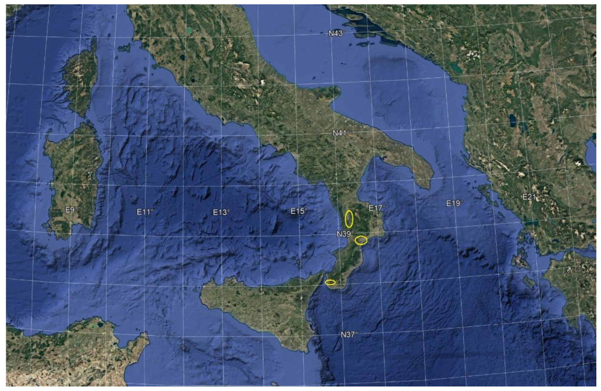
Figure 2.
(a) The course of the Crati river; (b) An image of the 1959 flood.
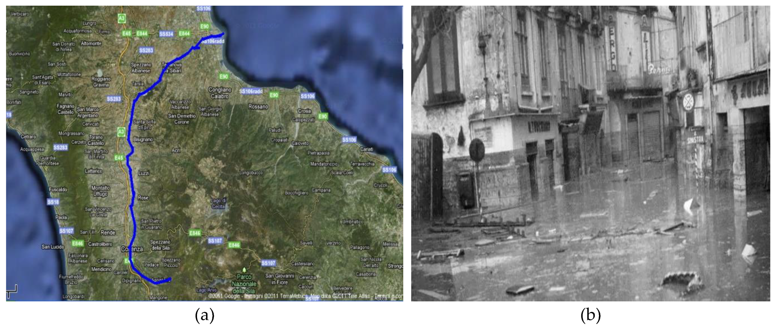
Figure 3.
(a) The course of the Corace river; (b) Bridge collapsed due to flood in 2010.
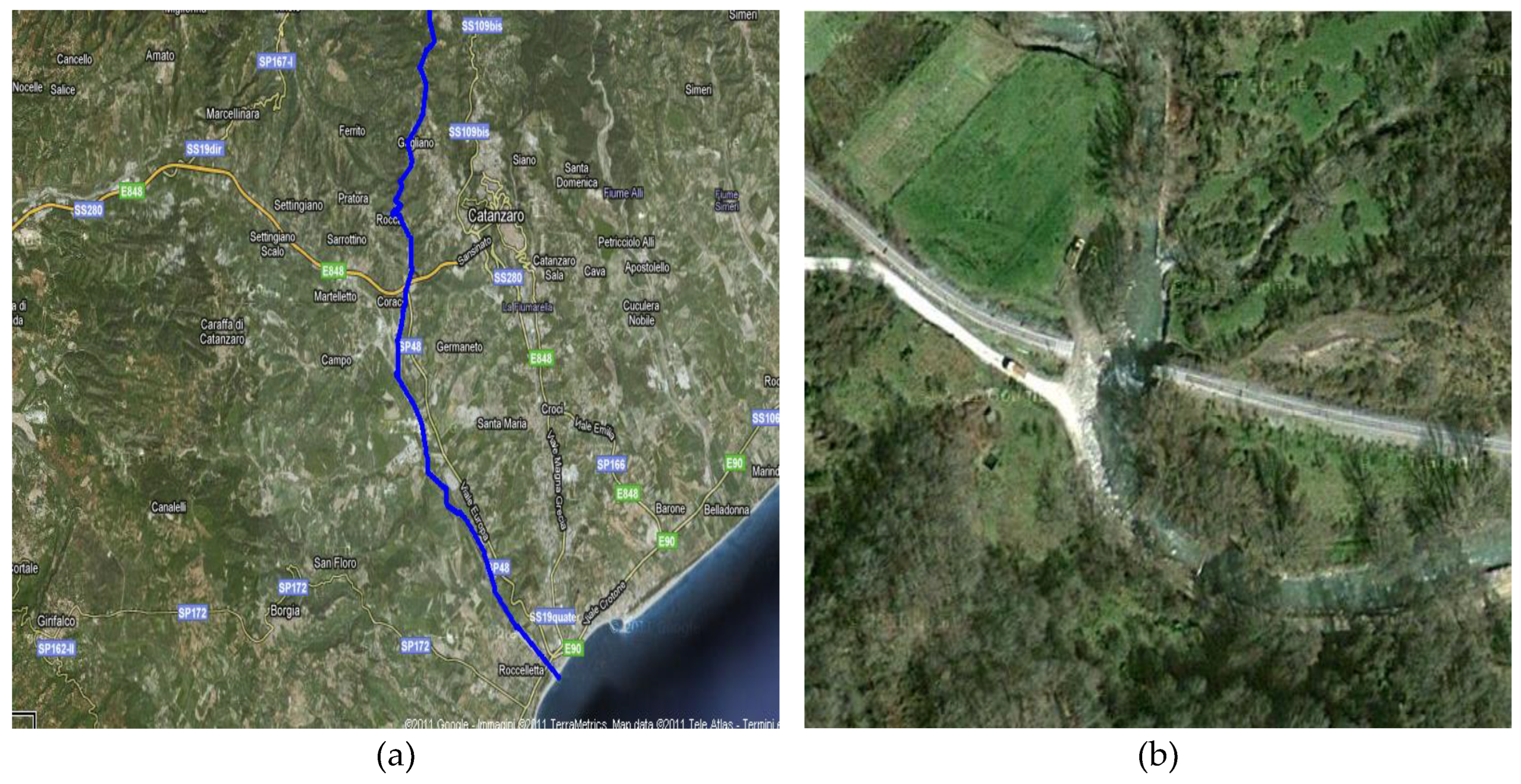
Figure 4.
(a) The course of the Valanidi stream; (b) Railway bridge collapsed due to 1953 flood.
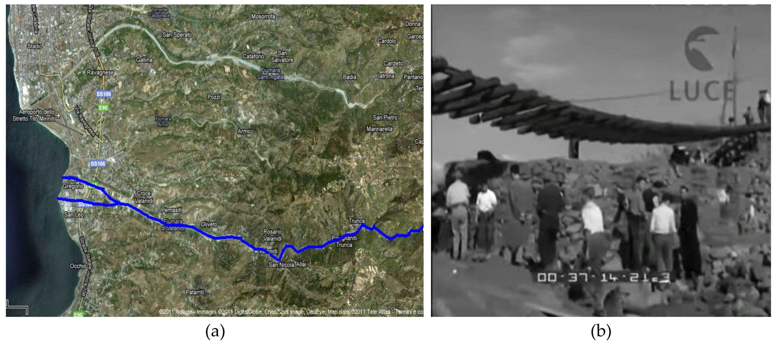
Figure 5.
The pipeline of the proposed modeling workflow.
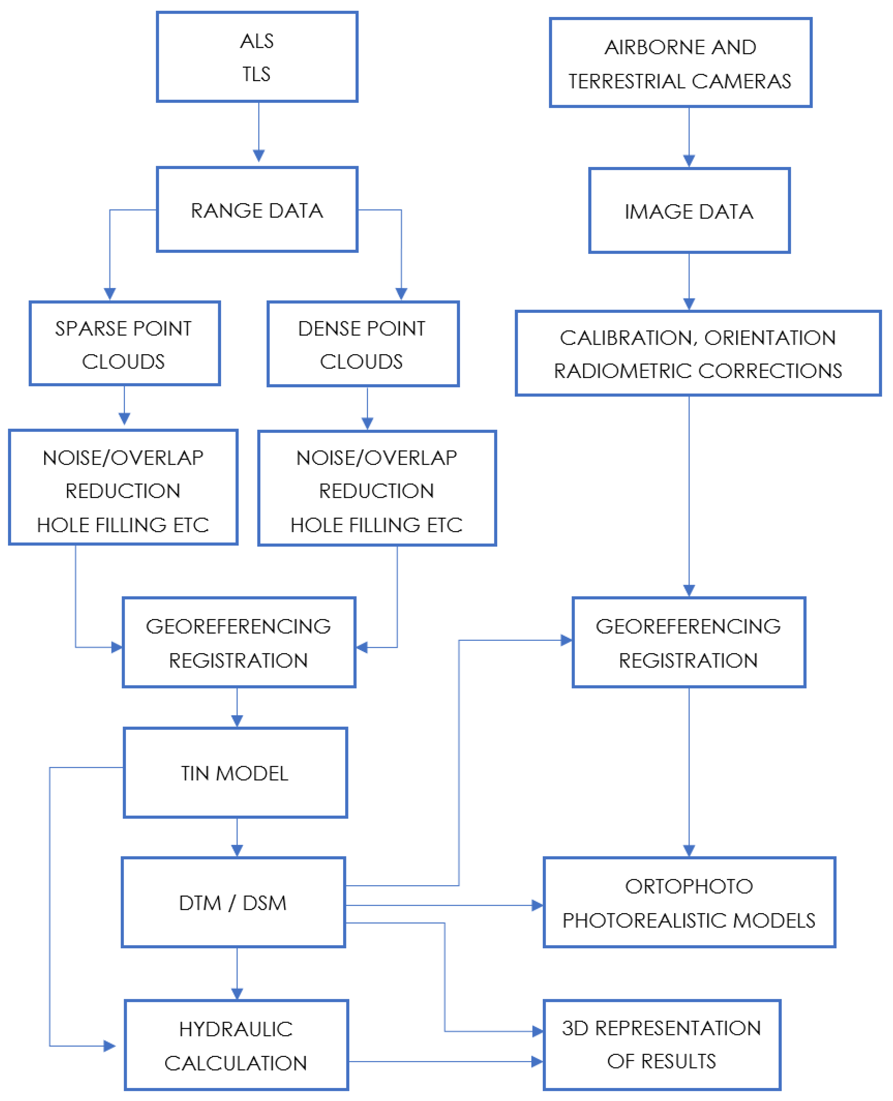
Figure 6.
(a) DSM of Crati river, at the confluence with the Busento river; (b) DTM section of the same area.
Figure 6.
(a) DSM of Crati river, at the confluence with the Busento river; (b) DTM section of the same area.
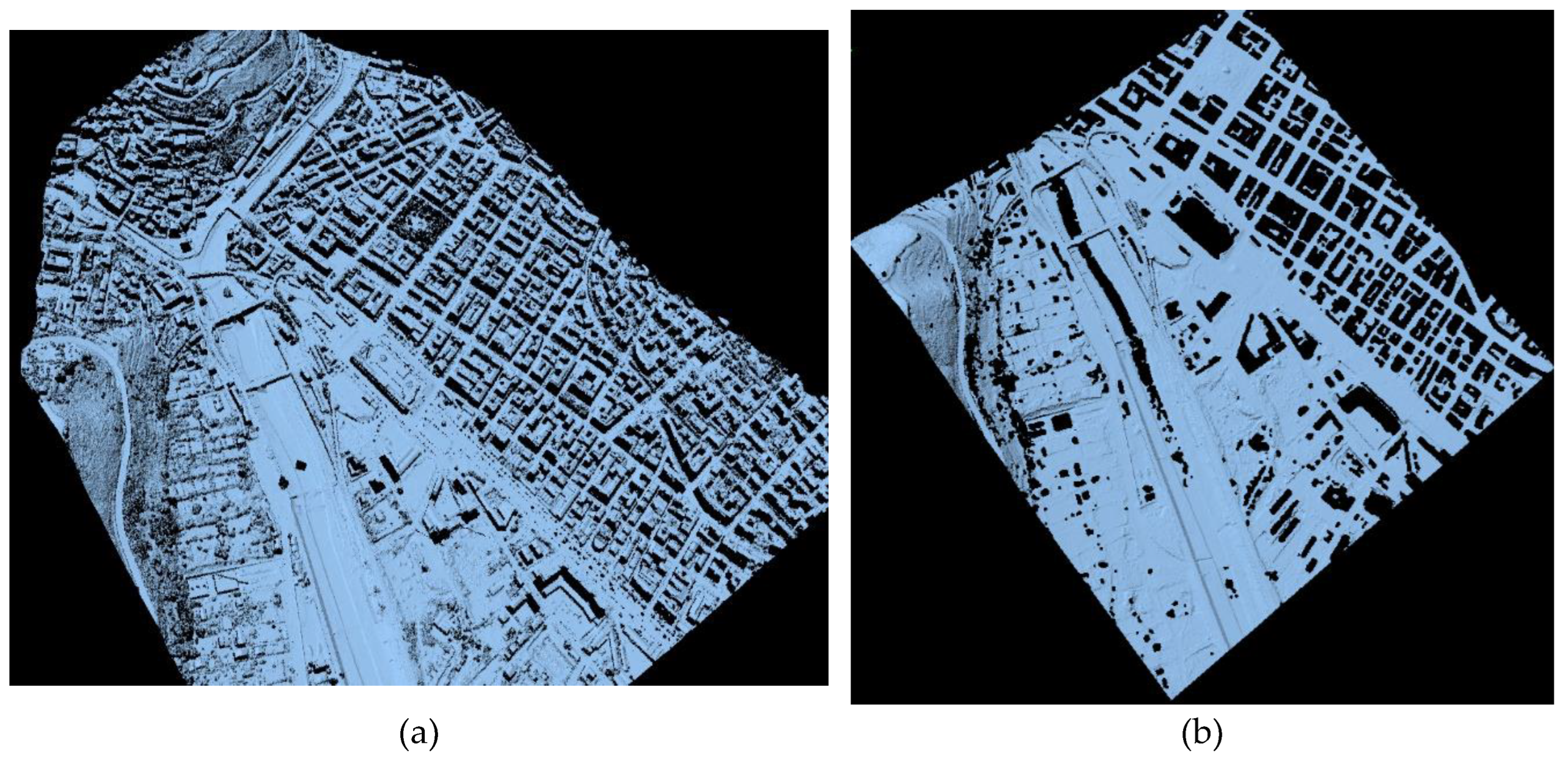
Figure 7.
(a) GCP on a riverbank parapet of Crati river; (b) GCP on a road sign near Corace river.
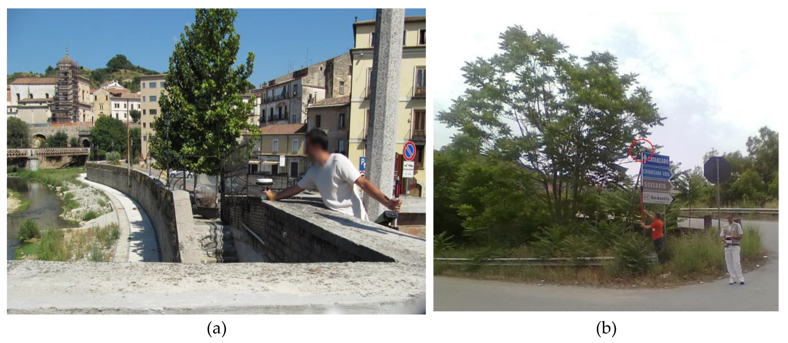
Figure 8.
(a) GCP on a log in the Corace riverbed; (b) The same GCP in the point cloud. The purple dots on the shore are those acquired via ALS, as are the dots visible in the shadow area under the vehicle hosting the TLS.
Figure 8.
(a) GCP on a log in the Corace riverbed; (b) The same GCP in the point cloud. The purple dots on the shore are those acquired via ALS, as are the dots visible in the shadow area under the vehicle hosting the TLS.
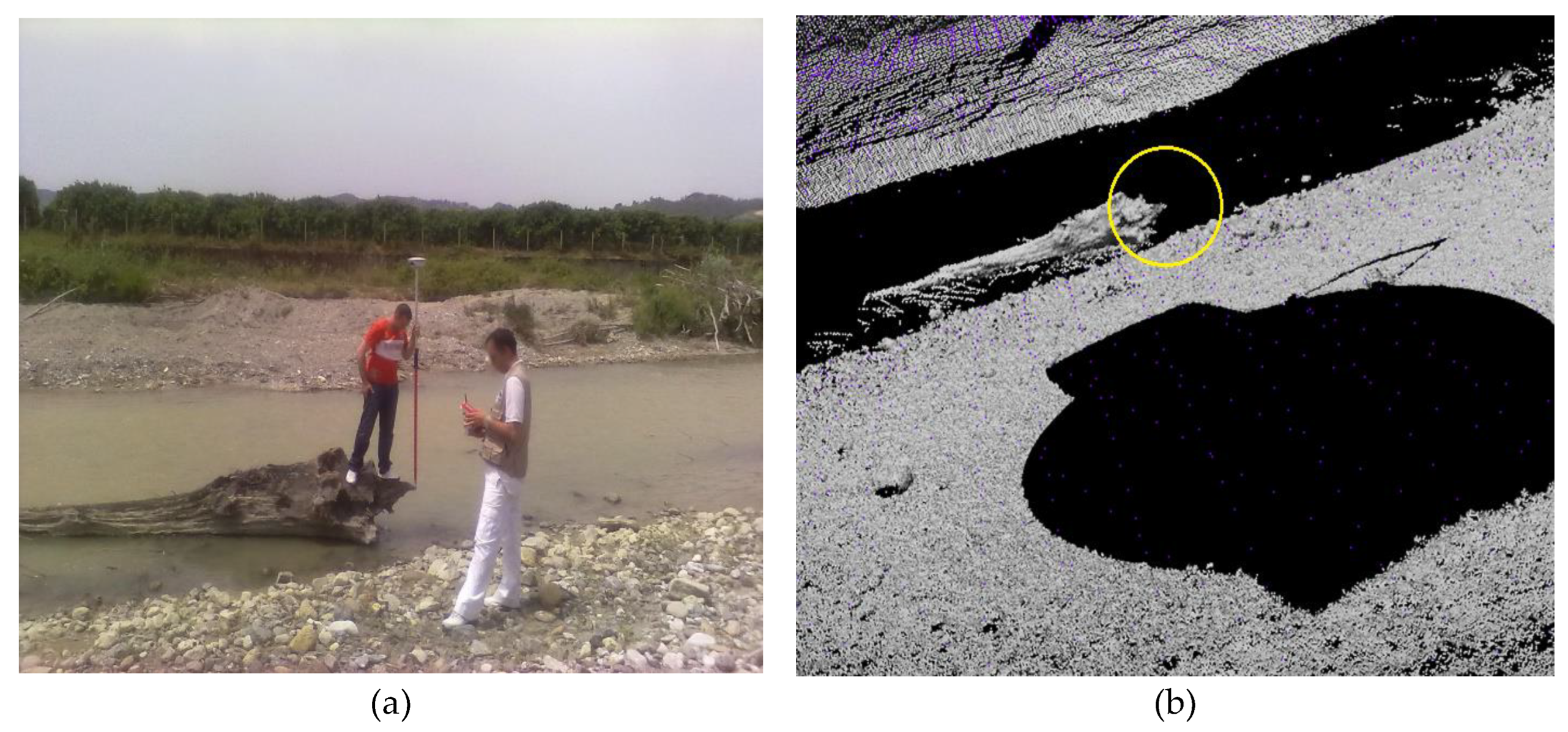
Figure 9.
The surface of a bridge deck used for registration. In green the TLS point cloud, in black the ALS one.
Figure 9.
The surface of a bridge deck used for registration. In green the TLS point cloud, in black the ALS one.
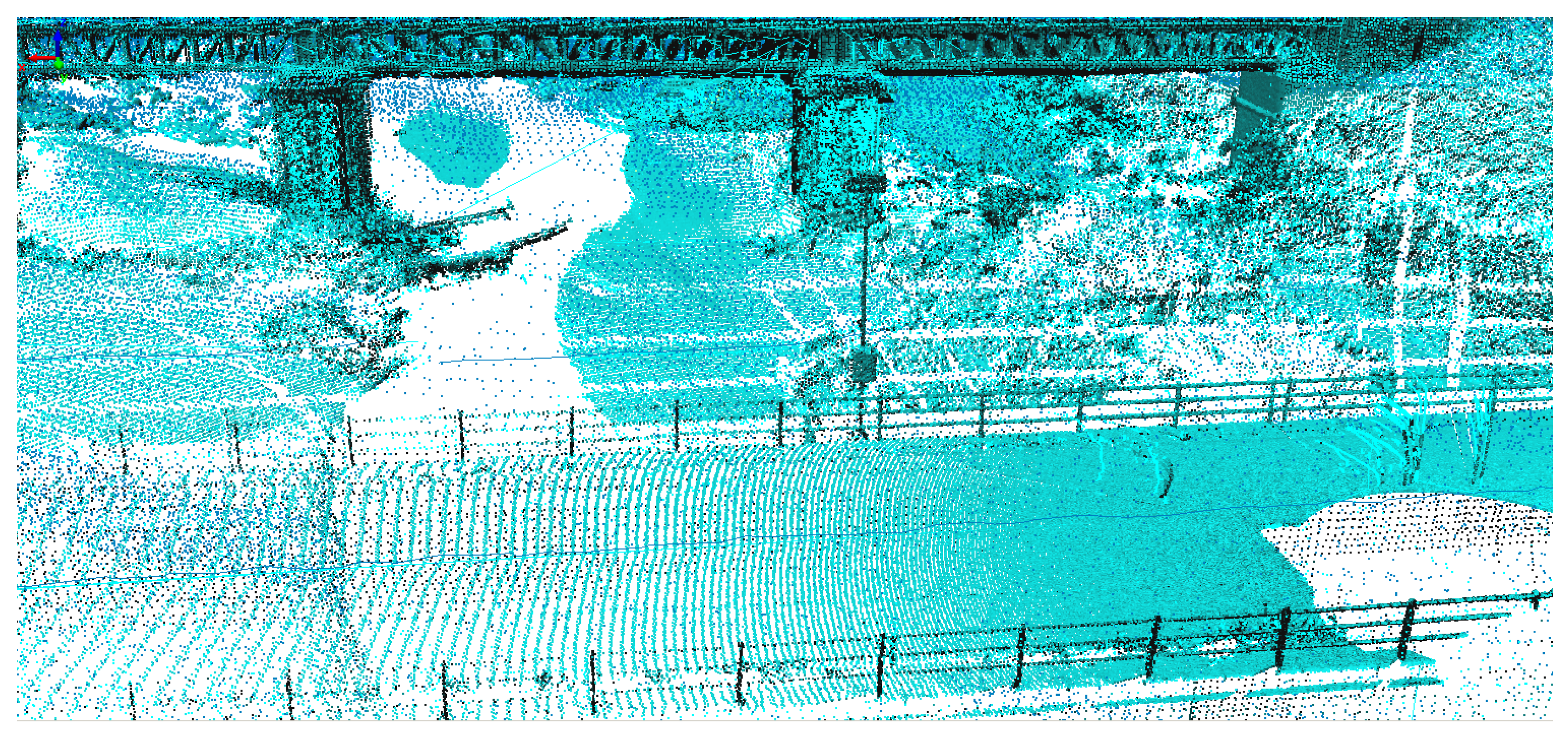
Figure 10.
The orthophoto of the middle stretch of the fiumara Valanidi.
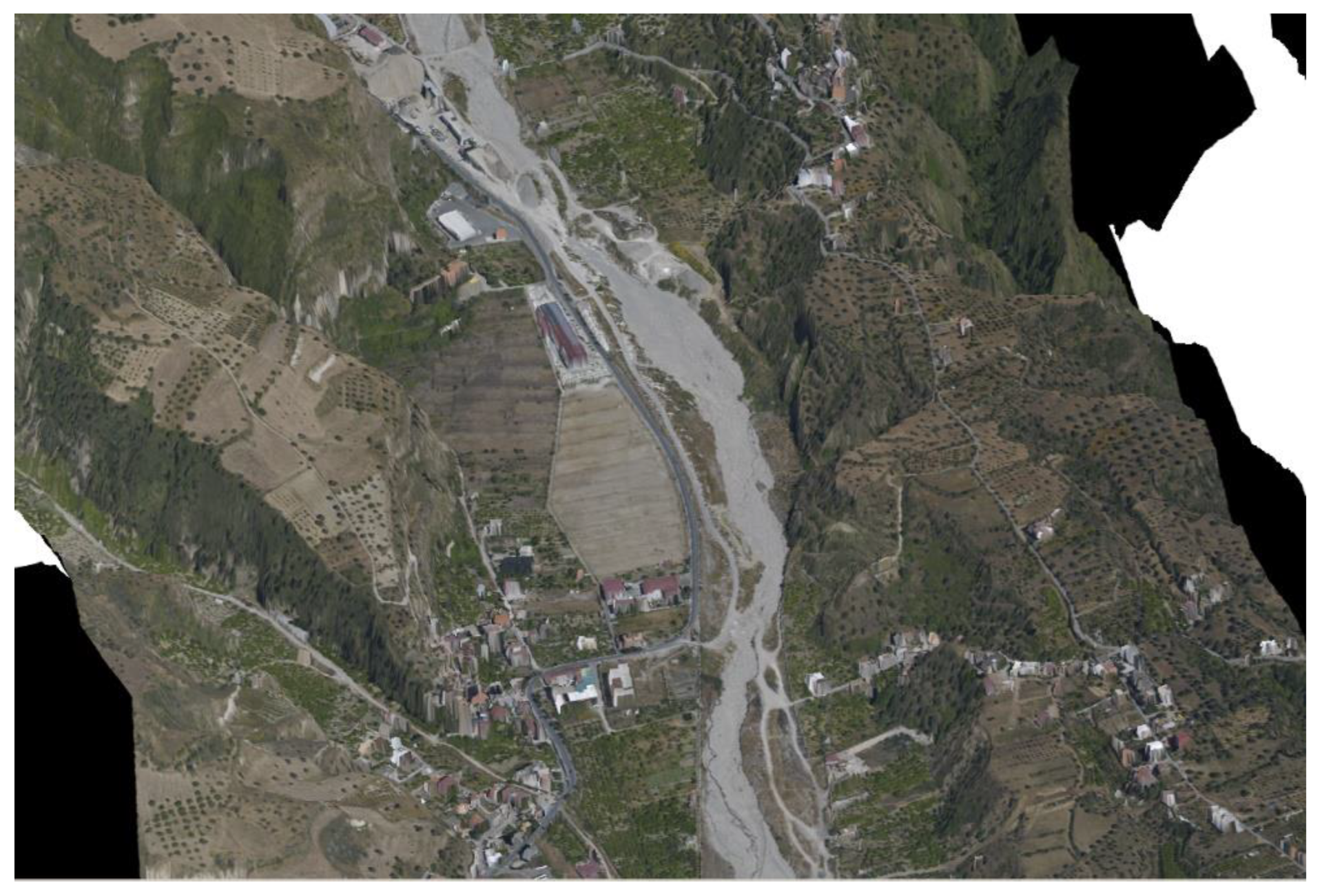
Figure 11.
(a) The meshing of ALS and TLS point clouds in the middle stretch of the Corace river; (b) A different perspective of the same river stretch.
Figure 11.
(a) The meshing of ALS and TLS point clouds in the middle stretch of the Corace river; (b) A different perspective of the same river stretch.
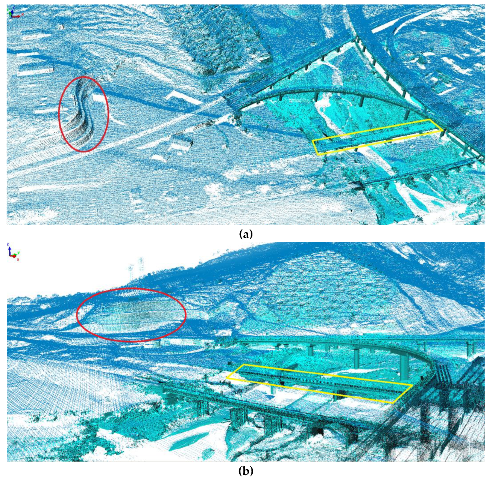
Figure 12.
(a) View of a bridge on the Corace river; (b) The TIN of the riverbed obtained from ALS point cloud; (c) The TIN tickening near the piles.
Figure 12.
(a) View of a bridge on the Corace river; (b) The TIN of the riverbed obtained from ALS point cloud; (c) The TIN tickening near the piles.
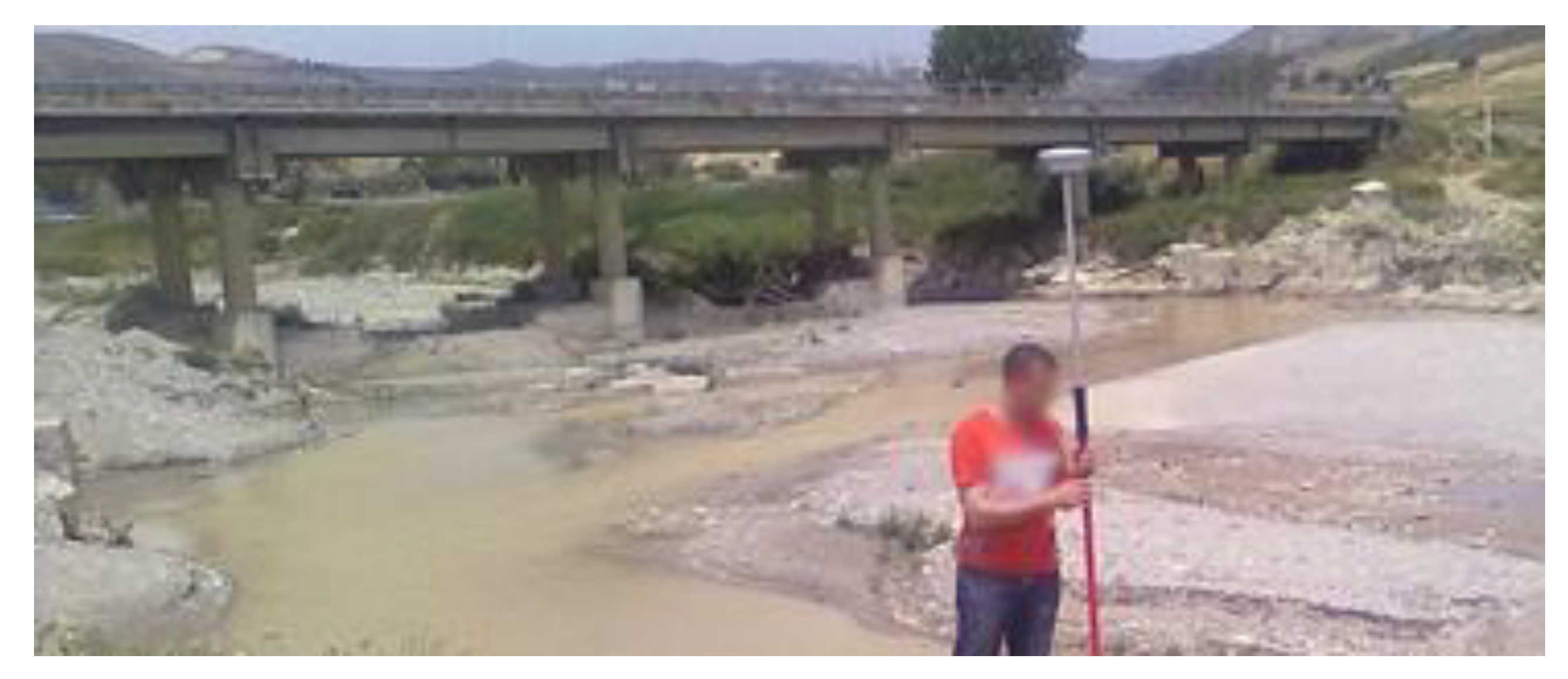
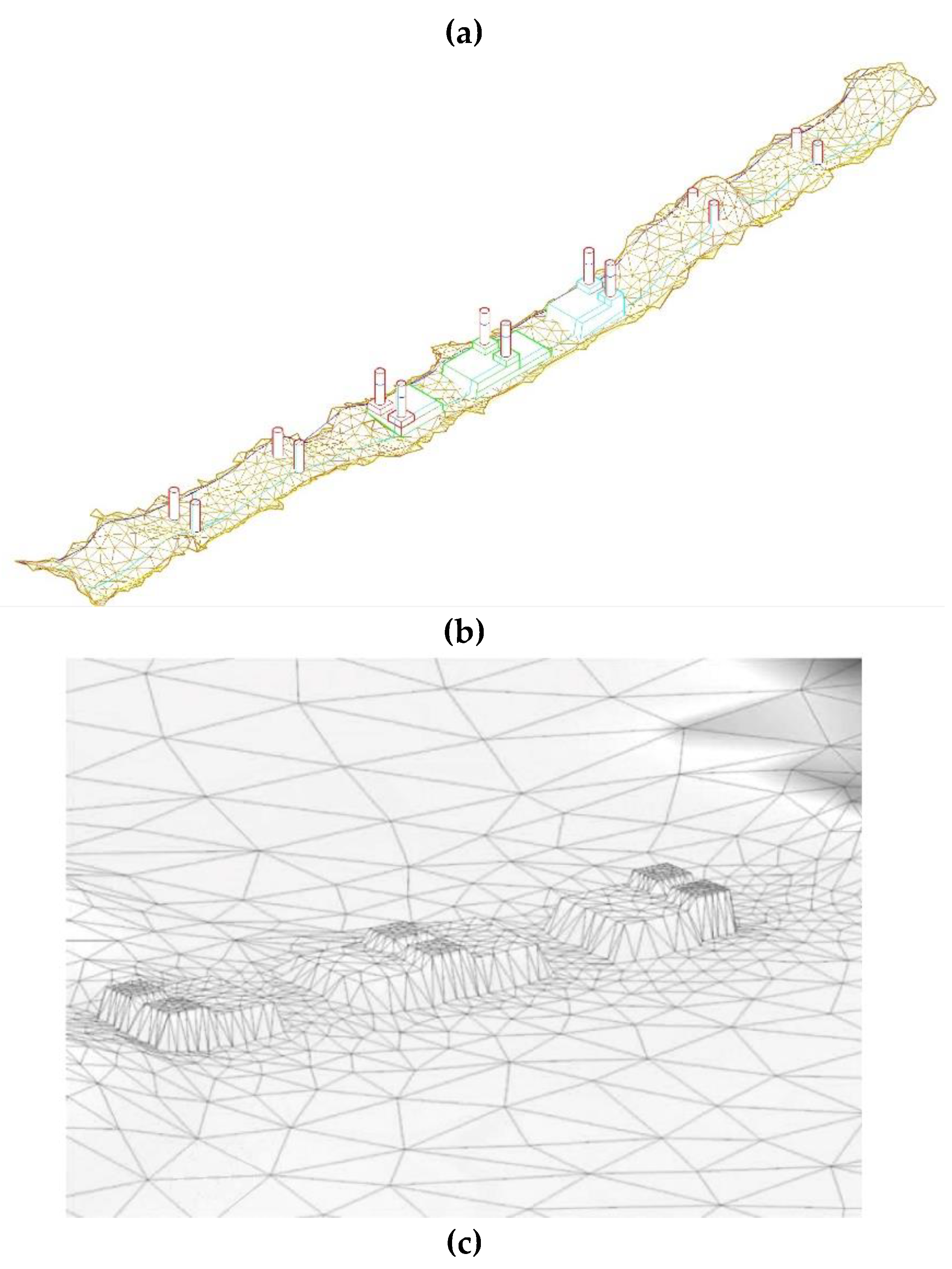
Figure 13.
(a) 2.5D model of the fiumara Valanidi with superimposed flow velocity (m/s) in a colour scale; (b) enlargement of the middle stretch.
Figure 13.
(a) 2.5D model of the fiumara Valanidi with superimposed flow velocity (m/s) in a colour scale; (b) enlargement of the middle stretch.
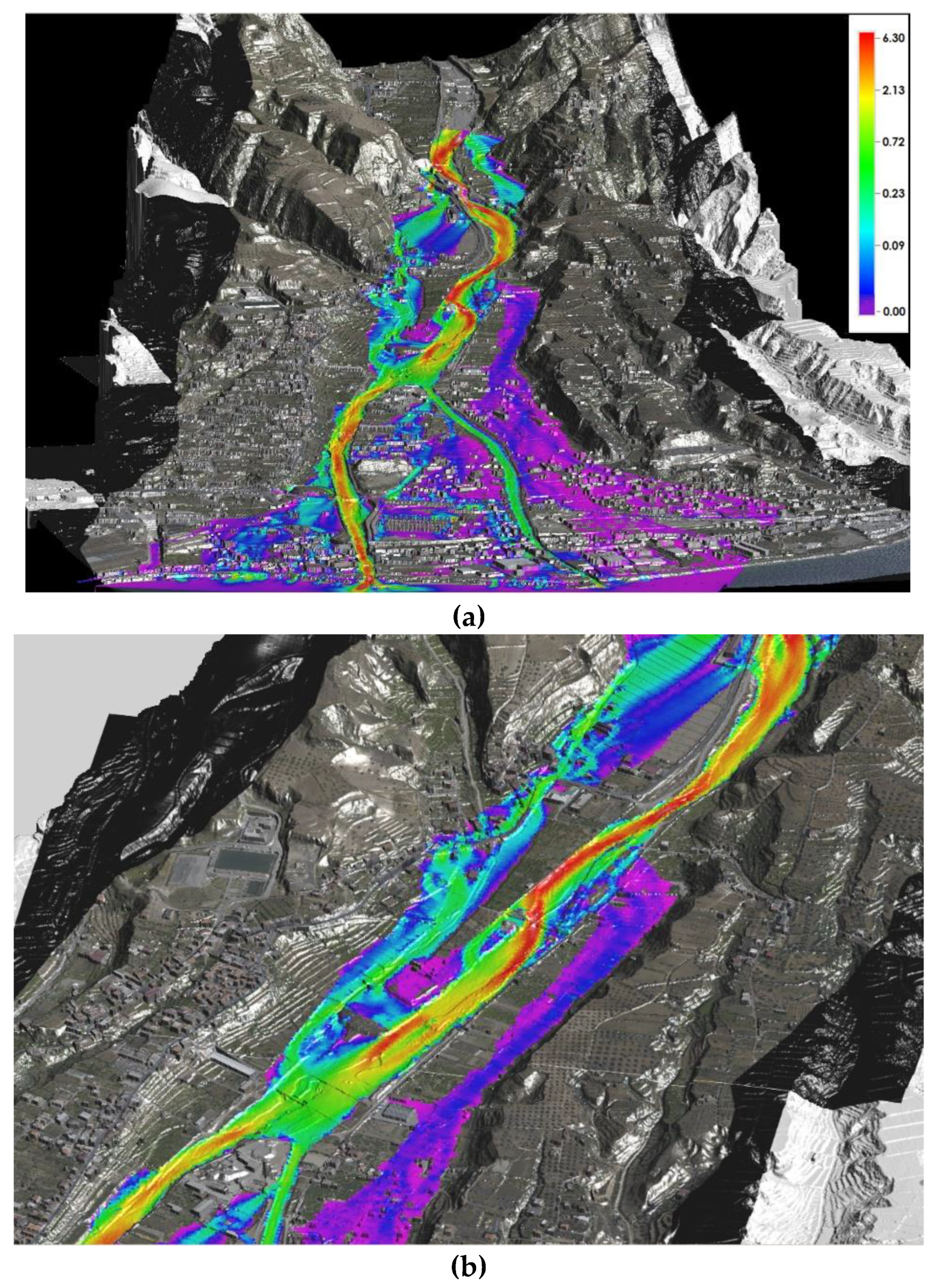
Figure 14.
A section of 1:5,000 scale cartography of the fiumara Valanidi area, with superimposed Eta values (m).
Figure 14.
A section of 1:5,000 scale cartography of the fiumara Valanidi area, with superimposed Eta values (m).
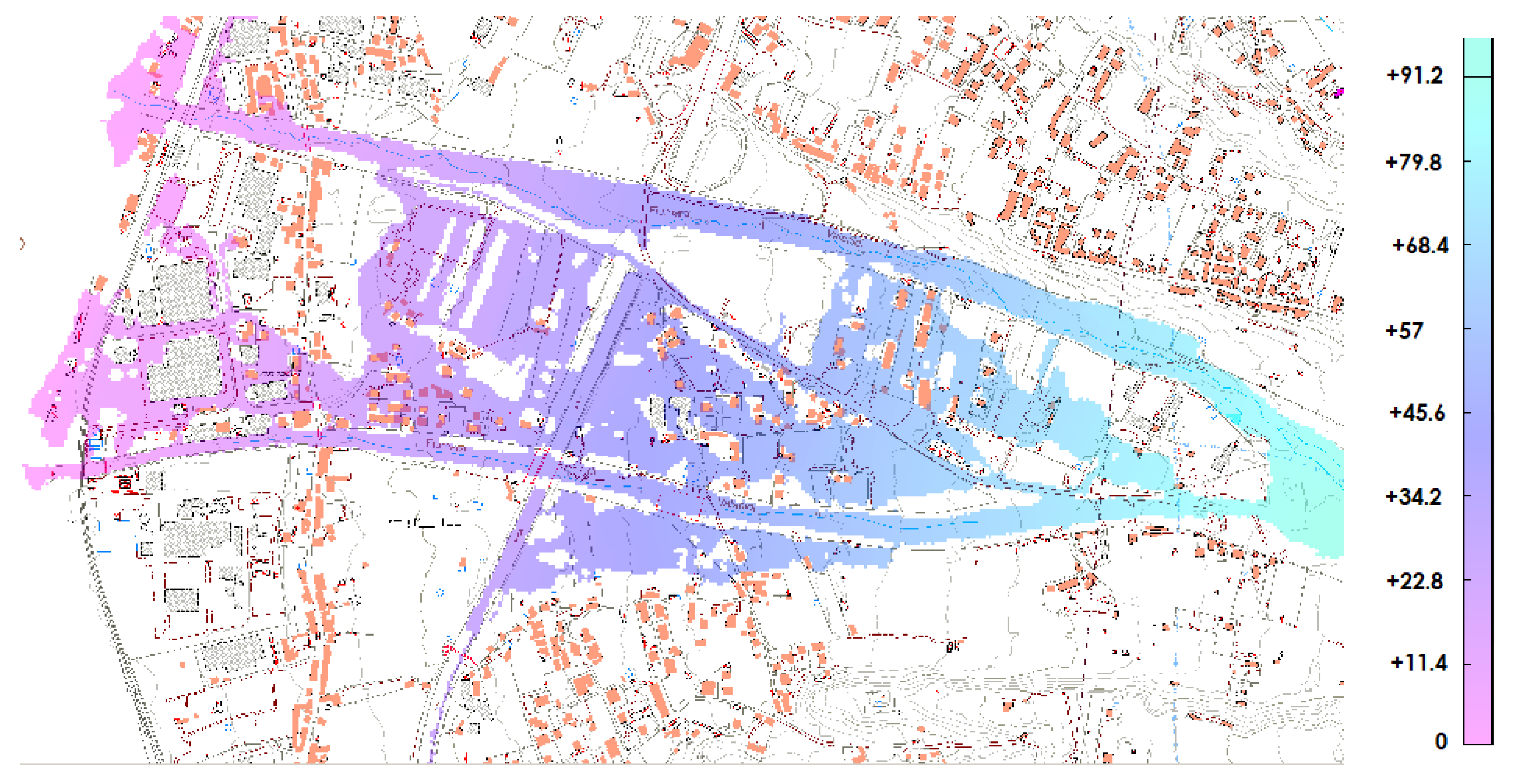
Figure 15.
(a) Representation of the deposition at the mouth of the Valanidi on the orthophoto with 5m GSD (m); (b) Same theme on the orthophoto with 1m GSD.
Figure 15.
(a) Representation of the deposition at the mouth of the Valanidi on the orthophoto with 5m GSD (m); (b) Same theme on the orthophoto with 1m GSD.
Disclaimer/Publisher’s Note: The statements, opinions and data contained in all publications are solely those of the individual author(s) and contributor(s) and not of MDPI and/or the editor(s). MDPI and/or the editor(s) disclaim responsibility for any injury to people or property resulting from any ideas, methods, instructions or products referred to in the content. |
© 2025 by the authors. Licensee MDPI, Basel, Switzerland. This article is an open access article distributed under the terms and conditions of the Creative Commons Attribution (CC BY) license (http://creativecommons.org/licenses/by/4.0/).
Copyright: This open access article is published under a Creative Commons CC BY 4.0 license, which permit the free download, distribution, and reuse, provided that the author and preprint are cited in any reuse.


