
Submitted:
23 January 2023
Posted:
25 January 2023
You are already at the latest version
Abstract
The 1884 Andalusia Earthquake, with an estimated Magnitude between 6.2 and 6.7, is one of the most destructive events that shook the Iberian Peninsula, causing around 1200 casualties. Ac-cording to paleoseismology studies and intensity maps, the earthquake source relates to the nor-mal Ventas de Zafarraya Fault (Granada, Spain). Diverse studies registered and later analyzed hydrological effects, such as landslides, rockfalls, soil liquefaction, all-around surge and loss of springs, alterations in the phreatic level, discharge in springs and brooks, and well levels, along with changes in water properties. Further insight into these phenomena found an interplay be-tween hydro-geomechanical processes and crust surface deformations, conditions, and properties. This study focuses on analyzing and simulating the features involved in the major 1884 event and aims at elucidating the mechanisms concerning the mentioned effects. This ex-post analysis builds on the qualitative effects and visible alterations registered by historical studies. It encompasses conceptual geological and kinematic models, and a 2D finite element simulation to account for the processes undergone by the Zafarraya Fault. The study focuses on the variability of hy-dro-geomechanical features and the time evolution of the ground pore-pressure distribution in both the preseismic and coseismic stages, matching some of the shreds of evidence found by field studies. This methodology can be applied to other events registered in the National Catalogues of Earth-quakes to achieve a deeper insight, further knowledge, and a better understanding of past earth-quakes.
Keywords:
hydrogeological effects
; hydro-geomechanical modelling
; Andalusia 1884 Earthquake
; pore pressure effects
; poroelasticity and seismicity
1. Introduction
The 1884 Andalusia Earthquake is one of the most destructive events that shook the Iberian Peninsula, involving around 1200 casualties, twice injured victims, destroying some 14000 homes and damaging other 13000 ones [1]. The tremor lasted around ten seconds, with an estimated Mw between 6.2 and 6.7 on the Richter scale, and had its focus between 10 and 20 km depth [2,3,4]. Diverse aftershocks followed the main shock during the very later days, some of them with rather notable intensity.
The 1884 earthquake was felt in an area of 120 x 70 km², affecting about one hundred urban centers in the provinces of Granada and Málaga. The most affected areas, with significant building collapses, deaths and injuries, were the Southwest of the province of Granada and the East of the province of Malaga. Arenas del Rey was the most affected population: 90% of the houses collapsed, the rest suffered damages; 135 dead and 253 wounded people. This town was later rebuilt in the current location, a few kilometers away from the previous one. Alhama de Granada underwent the highest number of victims, 463 dead and 473 injured. More than 70% of the houses collapsed. Then a new quarter was built near the Hoya del Ejido. After the 1754 Lisbon earthquake, the only quake in the Iberian Peninsula with greater magnitude than the 1884 event occurred in 1954, with its epicenter in Granada. However, the destruction in this case was not as great. The tremor caused rock falls and landslides on slopes, aggravating the earthquake effects. The former also caused the formation of numerous cracks. In addition, the earthquake induced hydrogeological effects of diverse ranges [5,6,7].
On January 7, 1884, the Spanish Government appointed a committee to study the earthquake led by the mining engineer Manuel Fernández de Castro y Suero (1825-1895) [5]. They immediately visited the region and distributed a 33-question survey including several queries about the alteration of sources, wells, rivers, etc. The French Academy of Sciences sent another commission, and so did the Italian Government and the Accademia dei Lincei [6], who sent seismologists Torquato Taramelli and Giuseppe Mercalli, who also provided an extensive report on the geology of the area with a map of the shake intensity [8]. The geologist José Macpherson y Hemas (1839-1902) explained that the earthquake mechanism was the movement along the faults that joined the Tejeda/Almijara massif to the North and South [7,9].
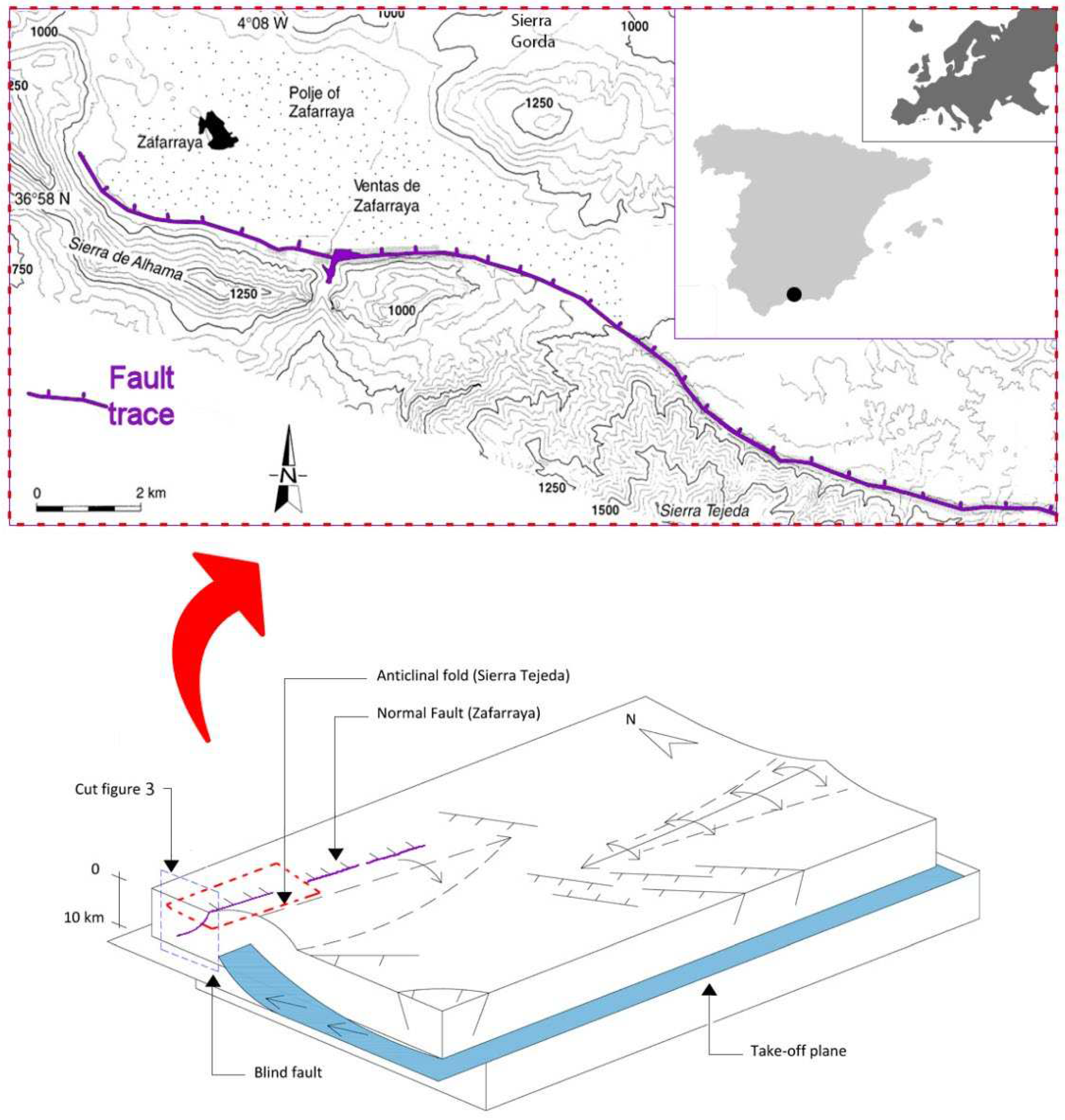
According to the most recent seismotectonic studies, the source of this earthquake is associated with the gravity fault of Ventas de Zafarraya (Granada, Spain). The trench study, to which the isosists are also adjusted, has evidenced such a source (Figure 1) [5]. During the recent Tertiary and Quaternary, the fault activity has entailed the subsidence of the area and the formation of a small and elongated graben, which in turn has originated the so-called Polje of Zafarraya. This polje is located in the southwest of the Granada Depression, is bordered to the N with the calcareous reliefs of Sierra Gorda and to the S with those of Sierra de Alhama. The polje borders on the SE with the metamorphic materials of Sierra Tejeda, so it lies in the contact between the external and internal regions of the Betic Range (Figure 1). Earlier studies reveal that the water table rose on the NNW side of the Zafarraya Fault and declined on the SSE region.
Further insight into these phenomena sheds light on the interplay between hydro-geomechanical processes and crust surface deformations, i.e., interaction among the water cycle, the tectonic layout conditions, and the crustal geomechanical properties.
Furthermore, the hydrogeological effects of the interaction between groundwater and earthquakes include soil liquefaction, mud volcanoes, geysers, all-around surge and loss of springs, increased discharge in springs and streams, changes in the physical and chemical properties of groundwater or its pressure distribution [10,11]. As we know, the hydrological variations due to earthquakes can affect several hundred kilometers around, and the processes can last for months or even years. These phenomena result from the interaction among hydrogeological processes, mechanical properties, and tectonic characteristics of the earth's crust due to earthquake-induced deformations. An earthquake causes changes in the stress state of the crust, decreasing with distance. Most of these hydrological alterations appear during and after the earthquake, and only in very few cases can they be foreshocks signs.
The catastrophic 1884 Andalusia earthquake gave rise to a notable number of damage reports published mainly during the next year in several European journals, bulletins of scientific societies, and books, authored by the most relevant geologists and seismologists from different European countries. Furthermore, three commissions were specifically designated to study this Andalusian earthquake [6,8]. Thus, the scientific community at that time could achieve new ideas about the nature of earthquakes and their relation with the geodynamic processes and geology of the region [12].
This 1884 earthquake also provoked numerous hydrogeological alterations that we have been able to collect. Despite the limited availability of quantified data on this historical earthquake, dated more than a century ago, the tectonically earthquake-induced fluid flows may have notable implications for our understanding of the kinematic behavior of the assumed source fault.
As is well known in empirical sciences, field observations precede first knowledge; then modeling takes place in attempting to replicate virtually the observed phenomena. Modeling is a slow, expensive and thankless task as it works with the systemic uncertainties of nature. Likewise, modeling is not deterministic, although it allows one to understand the complexity of the intertwined physical phenomena occurring in the complex subsurface system. Modeling enables making forecasts or estimates of extreme events and preventing risks. As prediction cannot build on empirical analyses, theoretical models must be used as the basis for strong motion forecasts. No surprise, geomechanical modeling of earthquakes, building on both observational and laboratory techniques, aims at shedding light on the seismic cycle predictions [13]. In such a case, it holds an enormous public service perspective, which is why the combination of observation and modeling can contribute to the advancement of scientific knowledge.
The complex interaction of coupled flow and geomechanics has received significant attention in engineering and the geosciences since decades ago [14,15,16]. Empirical observations reveal that earthquake faults occur within topologically complex, multi-scale networks driven by plate tectonic forces. Likewise, numerical modeling of the dynamics and earthquake simulations have shed light on both the occurrences of large earthquakes in a system of major regional faults and their recurrence times [17]. Thus, numerical methods provide insights into the seismic cycle, temporal and spatial earthquake clustering, and the occurrences of large events. Numerical simulations have become valuable tools to understand how both the different scales involved in earthquake physics interact and influence the resulting dynamics; and how the observable space–time earthquake patterns link to the essentially inaccessible and unobservable dynamics. [18]. In addition, those have also been used extensively in the context of fluid-injection-induced seismicity [19,20,21,22,23]. The debate spotlight has arisen recently from diverse industrial applications, such as large-scale geological CO2 sequestration [24,25], salt water or wastewater disposal [26], enhanced geothermal systems [27,28,29], hydrogen storage, enhanced oil recovery, and hydraulic fracturing during wells construction in the oil and gas industries [30,31].
Thus, the objectives of this work are the following:
- To describe and analyze the hydrogeological phenomena induced by the Andalusian earthquake of 1884.
- To establish a hydro-geomechanical conceptual model of the Zafarraya Fault that explains and allows understanding of these hydrological alterations.
- To implement a hydro-geomechanical numerical model to simulate the conditions of the massif surrounding the main fault during the pre-seismic and co-seismic phases. The results obtained from this simulation allow us to understand and explain the features and effects of the 1884 major event.
- To perform both matching and validation of both models.
This study focuses on simulating the hydro-geomechanical features involved by the 1884 Andalusia Earthquake and aims at elucidating the mechanisms that caused the mentioned effects. It encompasses a conceptual geological model, a kinematic one, and a numerical simulation procedure to account for the processes undergone by the Zafarraya Fault because of the major 1884 event. The two former comprise a 60-degree average Northward dip with a ten-kilometer-away outcrop level and a blind fault thrusting from SSE, causing a ground uplift in Sierra Tejada and hence a normal subsidence fault on the NNW side along with a graben formation, namely the Zafarraya Polje [32,33,34].
The numerical simulation procedure hereby used attempts to elucidate the rationale behind the 1884 event through a set of 2D finite element models to account for the hydro-geomechanical coupling and effects occurred in the sub-surface geologic domain. This approach addresses the coupling between poromechanical- and hydrological-constitutive behaviors of the ground surrounding the fault: effective normal stresses vary in space and time due to pore pressure changes, fluid flow and rock deformation, which may trigger the fault reactivation.
This procedure has already been applied previously to perform ex-post simulation analyses of subduction-zone earthquakes [35], seismic events caused by fluid injection at oil and gas production [23] or enhanced geothermal systems [36]. In addition, the same procedure became useful to evaluate how the injection rate may affect the fault reactivation [37], the influence of the ground viscoelastic properties or the inclusion of inertial effects in the injection-induced earthquake triggering [38].
The numerical models have undergone a preliminary calibration stage to account for the regional-specific conditions. Its results allow one to explain the source of fault displacements, understand the time evolution of the pore pressure distribution that occurred due to the 1884 event, and meet with some of the shreds of evidence found by field studies [39,40].
This numerical simulation procedure can be applied to other registered events in the National Catalogues of Earthquakes to grasp deeper insight, further knowledge, and a better understanding of past earthquakes. For instance, this procedure seems suitable for reviewing and updating the seismic focal parameters of past earthquakes recorded by the National Seismic Catalog.
In this regard, similar methodologies and the aid of new technology have proven valuable in understanding the possible reasons for past near-fault earthquakes that occurred elsewhere. It is worth mentioning the studies concerning the earthquake mechanisms in the 1703 Central Italy and 2009 L’Aquila (Italy) earthquakes [41,42], or to determine the seismic source characteristics of the 2017 Mw 5.5 Pohang earthquake (Korea) [28,43,44,45] and its relation to the Enhanced Geothermal System exploitation [28,43]. Indeed, modeling techniques still have the debate open whether this event was an induced earthquake [28,46] or just triggered [47].
Hence, numerical models, supported by experimental data and field observations, have become used increasingly to understand the rationale behind past earthquakes. Some examples worth mentioning are the seismic activity in the Tibetan Plateau over the last five centuries [48], the extent of the 1755 Lisbon Earthquake [49,50,51,52], or to gain insight into the focal parameters of the 2000 Saint-Ursanne Earthquake (Switzerland) [53], among other modelling applications for resembling past seismic phenomena.
2. Materials and Methods
2.1. Methodology
The methodology followed in this study comprises the following steps:
- Description of the hydrological alterations due to the 1884 Andalusia earthquake according to historical surveys.
The information on the earthquake-induced hydrogeological alterations stems from four sources, which sometimes refer to the same water points by adding or complementing the information. These sources are Surveys of the Spanish National Geographic Institute (IGN), the Committee of the Geological Map of Spain of 1884, the work of Domingo de Orueta, and the Spanish Commission (1885).
The IGN survey covered 66 towns (leaving aside farmhouses) in the provinces of Málaga, Granada, and Jaén. The Committee of the Geological Map of Spain refers to the alterations in the 11 most affected counties and towns. Seven of the most affected counties and villages appear in Domingo de Orueta's work [54]. In addition, the Spanish Committee's document described the alterations that occurred as well. Despite a long time, the surveys are rather extensive and offer reliability as it has been possible to carry out a quantitative analysis by relating them to the current geological and hydrogeological information about the region.
- Based on bibliographic background, the next stage seeks the setup of the geological and hydrogeological framework, and the seismotectonic characterization of the Zafarraya Fault surrounding area.
- Setup of a preliminary hydro-geomechanical conceptual model.
- The next stage involves the setup of a hydro-geomechanical 2D finite element plane-deformation model built on the conceptual one. Such a model accounts for the fully coupled phenomenon, i.e., the interplay among the fault friction, the existence of interstitial water in the pores, and a poro-viscoelastic medium. The ground is assumed homogeneous and isotropic, although it includes a heterogeneous initial stress field due to its tectonic history. The simulation considers the fault as a one-dimensional entity with a “slip-weakening” frictional response, i.e., its frictional resistance weakens when the relative slip between its edges is triggered [55]. Seismic rupture occurs when the acting tangential stresses reach the frictional resistance value at any part of the fault.
2.2. The Zafarraya Fault: Tectonic Context, Displacement and Recurrence Periods
This fault is located in the Betic Range and results from compressive and extensive deformations associated with the boundary between the Eurasian and African plates. The current average relative motion between both plates is 4 mm/year, which produces an oblique convergence in the NW-SE direction [56]. The study area belongs to the central-eastern sector of the Betic Range, whose current reliefs have evolved from the Tortonian to the present. The main structures identified in the region with recent tectonic activity are folds of kilometer size and E-W orientation, generally asymmetric and some with N vergence. Thus, these determine the formation of the main mountain ranges, such as Sierra Tejeda or Sierra Nevada. Besides, E-W and NW-SE orientation faults predominate in this sector, usually having a marked normal regime. In addition, the seismicity data indicate a main detachment level located between 10 and 20 km deep (Figure 1).
Field observations indicate that the over-15-km-long Zafarraya fault orientation varies between E-W, south of Zafarraya, and NW-SE, at the western end (Figure 1). The fault plane dips 60º -70º to the N, pitches 40º to the East (dextral-normal component), and shows several sets of normal striae. The total jump is several hundred meters and develops an endorheic basin, the Polje of Zafarraya, filled with sediments from the Tortonian to the present. This basin is asymmetric, with the depocenter displaced towards the fault zone.
On the southeast of the Zafarraya Fault, Sierra Tejeda shapes an antiform with a large E-W to ESE-WNW radius and a periclinal termination to the W. The development of the antiform has produced a positive relief parallel to the fold axis. The antiform southern flank is deformed due to SW-dipping WNW-ESE oriented faults (Type II faults), formed during the Neogene but without recent activity [57] (Figure 1). The geodetic network allows to quantify the current deformation in the Zafarraya Fault and the Sierra Tejeda Antiform.
Since the Middle Miocene, the simultaneous development and interplay between folds and faults developed. The presence of a detachment level with current seismicity, which approximately constitutes the fold compensation level, divides the crust into two blocks with diverse behavior (Figure 1). The crustal detachment activity is probably due to the NW-SE oblique shortening of the boundary between the Eurasian and African plates. The E-W oriented folds with N vergence could be related to the in-depth existence of oblique ramps or blind faults subparallel to the plate boundary and that it had a right-hand transpressive jump. The surface outcrop of normal faults subparallel to the fold axes, such as the Zafarraya fault, could be a consequence of the extension and collapse in the external arcs of the antiforms that constitute the main mountainous elevations.
Paleoseismic studies reveal that the recurrence intervals for earthquakes of M>6.5 are 2000-3000 years [58]. The mean minimum displacement of the fault is 0.17 mm/year for the post-Tortonian and 0.35 mm/year for the Holocene. New paleoseismic data, based on the analysis of fault trenches and radiometric dating, allow us to reconstruct the last 10,000- year seismic history of the Ventas de Zafarraya fault segment. Such studies have identified four major paleoseismic events () that can be considered as the maximum possible earthquake on this fault [59]. One of the main conclusions is that the average recurrence period of these "characteristic earthquakes" is around 2000 years. It is, therefore, one of the main active faults in southern Spain.
Figure 1.
Above: location of the study area and trace of the Zafarraya Fault, source of the 1884 Andalusia earthquake (Adapted from [60]). Below: tectonic schematic of the simultaneous development of folds with possible blind thrust faults and two normal fault systems in a detachment roof block. Type I faults, such as the Zafarraya Fault, would be produced by external arc extension and collapse of the antiforms that constitute the main E-SW reliefs. Type II faults would respond to the regional stress field with a NE-SW extension direction. (Adapted from [57]).
The Polje of Zafarraya is an endorheic depression, which suffers periodic floods [61]. The Polje spans about 10 km long by 3.5 km wide, nearly flat and surrounded by large reliefs. It limits to the N with the calcareous reliefs of Sierra Gorda, to the S with those of Sierra de Alhama, whereas to the SE with the metamorphic materials of Sierra Tejeda. The polje is filled in its southern sector by materials from the Upper Miocene (calcarenite and marl) disposed on the subbetic substratum. The Quaternary fill is above the Miocene materials in the polje central part, while the western sector is directly above the Mesozoic. These Quaternary alluvial deposits feature two differentiated levels, the lower one being more clayey [62]. Jurassic carbonate rocks outcrop on the West bordered by normal faults. Likewise, loamy-clayey materials appear in the south of these outcrops, which can belong to either the Cretaceous-Paleocene materials of the Zafarraya unit or the Colmenar-Periana Complex [62].
The Polje of Zafarraya is limited mainly by normal faults, among which the Ventas de Zafarraya fault outstands. Although no fault outcrops on the northern edge, geophysical studies and surveys suggest their existence. A recent gravimetric analysis has determined the basin sedimentary-infill geometric characteristics and identified some blind faults which fail to outcrop (Figure 1) [32].
Concerning hydrogeology, there are two aquifer systems in the area:
- Sierra Gorda Karstic Aquifer: it holds a free aquifer with Jurassic limestone and dolomite and a Keuper impermeable bottom. The carbonate formations are more than 1000 m thick. The average rainfall in the area is 840 mm. Its hydrogeological parameters are ; 𝑆=𝑚𝑒=1.5%.
- Polje of Zafarraya detrital aquifer: Made up of Miocene and Quaternary infill sediments from the basin, having a maximum thickness of 280 m. The upper Miocene and Quaternary sediments are about 60 m thick and include sandy and gravel alluvial deposits with clay intercalations. In general, this upper detrital aquifer feeds the limestone aquifer underneath, but sometimes the reverse happens due to heavy rains that flood the polje. The flow is directed mainly towards the NE, with a gradient of 0.085-1.7%. This aquifer is heavily exploited, with 400 wells, and the water table is shallow, less than 15m deep.
2.3. Hydrogeological Alterations: Types and Geographical Distribution
Thanks to the Spanish National Geographic Institute surveys, the information provided in 1884 by the Committee of the Geological Map of Spain, and the reports of Domingo de Orueta and the Spanish Committee (1885), it has been possible to characterize the hydrogeological alterations produced by the earthquake. These encompass soil liquefaction (in Vélez-Málaga), the appearance of new springs, loss of existing springs and lowering of the water table (in Sierra Tejeda), persistent increase in discharge in springs and streams (the Alhama thermal spring), variations in well levels, in the physical and chemical properties of groundwater, in pressure [58,63,64].
Thus, the mentioned historical documentation states that the frequency and intensity of the alterations occurred around the epicentral area. Furthermore, the water table rose in the fault NNW near-field and broadly declined in the SSE region. Figure 2 depicts a schematic representation of the diverse hydrogeological alterations, the localities, and areas where these effects occurred.
2.4. 2D Geological Model of the Fault
The conceptual geological model represents the Zafarraya fault with a varying dip around 60º to the North, a detachment level 10 km away, and a blind thrust fault (Figure 3). The kinematic model depicts this blind fault pushing to the SSE, then producing an uplift of Sierra Tejeda and consequently a normal subsidence fault to the NNW, with the formation of a graben, the Polje of Zafarraya [32,33,34].
2.5. Coupled Physics Included in the Simulation Model
The numerical analysis of the effects caused by earthquakes in the earth's crust needs to consider the coupling among the distinct physical processes involved: the fluid flow through the porous medium, the poromechanical ground response, and the fault frictional behavior. The procedure implemented here accounts for the interplay among those three physics (Figure 4). However, it becomes necessary to adopt assumptions and simplified formulations because of the complexity of the laws that govern each physical process.
The numerical simulations require two types of discretization: time discretization and finite element assemblage. Likewise, the numerical solution of the equations governing the whole system response also requires a specific procedure, not to mention the time step variability suitable to search for the time response. The time solution procedure monolithically solves the values of the pore-fluid pressure evolution, the ground deformations, and the frictional state in the fault. Such simulations are computationally demanding, due to the contrasting spatial and temporal scales involved: they range from months for interseismic periods down to milliseconds for the dynamic rupture phase.
The 2D numerical model assumes a state of plane strains and that these can be considered infinitesimal. The former also considers the ground a homogeneous linear poro-viscoelastic medium.
The linear elastic properties of the homogeneous material considered are the modulus of elasticity and Poisson's ratio.
The governing differential equations comprise the internal equilibrium of the solid, the fluid flow, and the storage equations.
The linear-poroelasticity theory equations are the linear constitutive relations of the porous medium, the internal equilibrium equations, and the mass balance equations in the fluid. The set of equations describes the coupling between the fluid flow and the elastic mechanical response of the porous medium. Those assume the principle of effective stresses, which relates the intergranular forces in the solid skeleton and the pore pressure, , through the Biot-Willis parameter, . By considering positive both the tensile stresses and pore pressures greater than atmospheric, this principle reads:
Terzaghi first formulated this principle with . In the above equation are the total stresses, wheras is the Kronecker Delta, and are the effective stresses, defined by
In this equation, is the Lamé constant, is the volumetric deformation of the porous material, and is the shear modulus of the porous medium, and are the strain components.
Biot (1941) first proposed the classic theory of linear poroelasticity; Rice and Cleary (1976) extended its formulation and posed solving in a coupled manner the evolution of pore pressure, , rock deformation, and friction at the fault contact [15,25]. The Biot equations of poroelasticity for the quasi-static case (i.e., the fluid and fluid-solid relative accelerations and velocities are disregarded) are as follows (storage equation) [65]:
In these equations:
- is the fluid (water) density.
- is the constrained specific storage coefficient, which represents the volume of water either extracted from or added to storage in a confined aquifer per unit area of aquifer per unit decline or increase in the piezometric head. This unknown coefficient needs to be estimated through a model calibration. When the solid phase consists of a single constituent, the constrained specific storage becomes [66,67]:
This study considers the canonical case with , then the storage coefficient is directly related to the fluid compressibility since becomes .
- is the intrinsic permeability of the porous medium .
- is the dynamic viscosity of the fluid.
- is the Cauchy stress tensor.
- is the bulk rock density, , and the dry rock density.
- is the gravity acceleration vector.
Equation (4) for the simplified dynamic case becomes:
with being the second time derivative of the displacement field u of the solid matrix, i.e. the acceleration field of the solid points.
3. Numerical Model Setup
The mechanical boundary conditions are: Vertical displacements are restrained at the bottom boundary; horizontal displacements are impeded at the right edge, whereas the far-field regional stresses act on the left edge (Figure 5a).
Besides, the system departs from an initial equilibrium state, in which the tectonic boundary forces, the gravity load, and the hydrostatic pressures are balanced. For effectiveness and accuracy, the model performs a dynamic analysis, i.e., including the inertial terms in the time response. The dynamic analysis involves the simulation of elastic wave propagation coupled to nonlinear friction at fault surfaces [68] and requires high-resolution spatial discretization and accurate time integration.
We initialize the model by solving the steady-state poroelastic layout of the saturated domain subjected to the far-field tectonic loads, frictional contact at the fault, no-flow boundary condition at the top boundary, and the hydrostatic pressure field elsewhere.
We have calibrated a simplified 2D model, which, when subjected to the average deformations of the interseismic period, causes the shear failure, the onset of slip and finally reaches the seismic rupture. The calibration entails the static equilibrium of the stress state; the fault is initially at rest, and there are some additional residual folding stresses in a region close to the assumed hypocenter. This implies that some part of the fault is at the verge of stability, i.e., the acting shear stress value is close to the shear strength, so this part of the fault is prone to nucleate the earthquake (Figure 5b). The method helps explain the fault slip during the Andalusian earthquake and the pore pressure evolution within the medium and on the free surface.
3.1. The Fault Frictional Model
The fault frictional constitutive law accounts for the relative slip between both edges. The fault is initially at rest, so the acting shear stresses are lower than the shear strength of the fault contacts, . Fault reactivation occurs when the effective normal-stress changes cause the acting shear stresses to reach the frictional resistance at any fault point. The Mohr-Coulomb law controls this issue:
In the above equation:
- is the shear resistance at any fault point.
- is the cohesion term of the resistance, neglected in this study.
- We include a radiation damping term that acts as a velocity-dependent cohesion, , in the definition of fault strength to resolve the rupture dynamics. Then we consider a damping factor , with being the shear wave speed. The phenomenon of radiation damping accounts for the volumetric dissipation mechanism of seismic waves, in the form of a velocity-dependent cohesion, in the definition of the friction resistance of the fault [65,69,70].
- is the friction coefficient of the contact.
- is the effective contact (normal) pressure at any fault contact point. It is given by , with being the contact pressure between the fault edges (compressive pressures are positive). Its value is chosen as the maximum on both sides of the fault, [71]. The fault remains locked when the shear stress acting on the fault, , is lower than the frictional strength, ; otherwise, it slips.
Besides, we assume a slip-weakening friction law for the fault, i.e., the friction coefficient value decays upon fault reactivation. So the friction coefficient shifts from the at-rest conditions, i.e., its static value, , to the dynamic value, , after a distance , i.e., the critical slip weakening distance —a property of the fault’s friction law— [55].
The numerical model assumes that the fault is rather transversely permeable, whose hydraulic flow [] between its edges is simplified by a transverse permeability coefficient of . We model flow across the fault through a simple mass flux exchange between the two contact surfaces defining the fault. Denoting by the pressures on either side of the fault and by the inward mass fluxes per unit area, we approximate the latter through an effective fault transmissibility, , as
The above jump condition couples the pore pressures on both sides of the fault, allowing a transition from essentially no-flow towards pressure continuity as increases.
3.2. The Ground Model and Properties
A battery of simulations with diverse configurations has been performed to calibrate the numerical model. The necessary confinement stresses are applied to the vertical edges so that the system is in static equilibrium at the beginning of the seismic cycle, which encompasses the corresponding stress state plus the natural settlements of the ground due to consolidation (Figure 6).
To calibrate the model, various parameters are varied, such as the porosity of the medium, variable with depth between 1% and 5%, and the intrinsic permeability, , linearly decreasing with depth, ranging between (free surface) and (bottom). Also, the dimensions of the diverse trial domain models have ranged between up to .
The elastic modulus of the porous medium is estimated to be around , its Poisson's ratio is , and its dry density is .
We assume that the porous medium is viscoelastic, according to the Kelvin-Voigt formulation, with a viscosity coefficient of . This parameter value has been calibrated, since large values lead to undesired artificial damping of the dynamic response. The Biot Willis coefficient value is , so there is full coupling between pore pressure variations and the deformability of the porous medium [15]. The dynamic viscosity of pore water value is , and its compressibility is .
3.3 The Finite Element Domain
The domain is a 1-meter-thick rectangle with a depth of 14 km and a length of 28 km (Figure 6). The initial stress state includes a non-uniform distribution due to its tectonic history.
The finite element mesh is an unstructured grid of triangular Taylor-Hood elements. The mesh is highly refined along the fault, with the aim of resolving the rupture propagation fronts. The minimum element size is 4m along the fault zone. The interpolation functions are quadratic for displacements and linear for pressures.
4. Results and Discussion
The conceptual model developed includes the most significant phenomena that may have led to the seismic event. This study has simplified the complexity of features arising from ground heterogeneity and the number of faults. Thus, the fault more likely to slide has been modeled. Indeed, the target zone is the area near the hypocenter to capture the seismic rupture.
In the pre-seismic phase, before the slip, the south zone of the fault is compressed by the effect of both the normal fault activity and the pushing lower detachment, which also compresses the ground. Conversely, the opposite occurs in the valley area, northward of the fault, since the zone is under tension and the pores are saturated.
In the co-seismic phase, once the fault shear resistance is reached triggering the earthquake, the valley area sinks and shrinks, closing the previously open pores and expelling the water, thus originating new sources and other hydrogeological alterations. The results of this study simulate these described effects in a similar way to what happened.
The calculated surface settlement on the fault's left side is around 20cm. On-fault pore pressure controls dynamic fault weakening and strengthening in numerical models [72,73]. The maximum overpressures affect the water table level; hence, the red area near the surface left side of the fault indicates the appearance of new springs (Figure 7-b). Figure 7 illustrates the earthquake patch (a) and the overpressures induced by the fault instability and the time of rupture.
Figure 8 features the patch growth in terms of fault-tangential slip velocities (a) and relative displacements between edges (b).
The simulation yields that the patch size becomes nearly 9024m, with an average relative slip of 0.2181m, yielding a scalar seismic moment per unit thickness is .
The present study focused on developing and evaluating a computational model to simulate past earthquakes in view of their qualitative hydrogeological effects. An important next step builds on applying the proposed simulation framework to explore the relationship among hydrogeological sequels, hydro-geomechanical properties, frictional constitutive parameters, and the estimated earthquake magnitude.
The drawback of this type of retrospective study is the lack of reliable estimates for the model parameters. Indeed, their values have to be adjusted so that the results obtained are as similar as possible to the effects observed, for example, settlements or elevations, the surge and loss of springs and streams, among others.
5. Conclusions
The implemented conceptual model is valid to explaining the event that occurred in 1884. Undoubtedly, this model would lead to more accurate results if additional field data were available, such as regional stress fields, folding issues, and hydrostatic/water pressure data, geomechanical conditions in the vicinity of the hypocenter, among others.
On the one hand, this simplified methodology helps to understand the role that pore pressure plays in triggering the earthquake. The influence of the fluid pressure field in earthquake rupture is not negligible, as pore pressure variations induce changes in the effective normal stresses on the fault, thus may leading to exceed its shear resistance. When the fault stress state is close to the critical equilibrium configuration, changes in pore pressures can trigger the fault reactivation.
On the other hand, the application of this type of models is transversal: it can provide better knowledge of the National Earthquake Catalogs. Indeed, the collection of records of the hydrogeological alterations produced by historical earthquakes may supply a practical information to understand better the conceptual models and calibrate simulation models. Hence, these models can help us understand how seismicity and hydrogeological alterations seldom occur.
Author Contributions
Conceptualization, E.S. and J.C.-M.; methodology, E.S. and J.C.-M.; software, M.M.-H.; validation, M.M.-H. and J.C.-M.; formal analysis, E.S., M.M.-H. and J.C.-M; investigation, E.S. and J.C.-M.; resources, E.S.; data curation, J.C.-M. and M.M.-H.; writing—original draft preparation, E.S., M.M.-H. and J.C.-M.; writing—review and editing, J.C.-M.; visualization, J.C.M.; supervision, E.S., M.M.-H. and J.C.-M.; project administration, M.M.-H. and E.S; funding acquisition, E.S., M.M.-H. and J.C.-M. All authors have read and agreed to the published version of the manuscript.”
Funding
This research was funded by the Universidad Politécnica de Madrid through the Educational Innovative Programme 2021–2022, Project codes IE22-0403.
Data Availability Statement
The data presented in this study are available from the authors upon request.
Acknowledgments
The authors gratefully thank the professors Sandro Andrés, Luis Cueto-Felgueroso and David Santillán for their technical support in the software implementations.
Conflicts of Interest
The authors declare no conflict of interest.
References
- Quidam, U. (1885) Cartas desde los sitios azotados por los terremotos de Andalucía. Lib. Nac. y Ext. Madrid, 142. Available at: https://digibug.ugr.es/bitstream/handle/10481/7943/c-019-036%20%2837%29.pdf?sequence=1&isAllowed=y.
- Lasala y Collado, F. (1888). Memoria del comisario regio para la reedificación de los pueblos destruidos por los terremotos en las provincias de Granada y Málaga. M. Minuesa de los Ríos, Impresor, Madrid. Available at: http://www.bibliotecavirtualdeandalucia.es/catalogo/es/catalogo_imagenes/grupo.do?path=150661.
- Fouqué, F. (1889). Estudios referentes al terremoto de Andalucía ocurrido el 25 de diciembre de 1884 ya la constitución geológica del terreno conmovido, hecho por la comisión destinada al objeto por la Academia de Ciencias de París.
- Botella y Hornos, F. D. Los terremotos de Málaga y Granada. Bol. Soc. Geográfica de Madrid, 1885, t. XVII, 30.
- Fernández de Castro, M.; Lasala, J.P.; Cortázar, D.; Tarín, J.G. (1885). Terremotos de Andalucía. Informe de la Comisión nombrada para su estudio dando cuenta del estado de los trabajos en 7 de marzo de 1885. Available at: http://hdl.handle.net/10481/19269.
- Taramelli, T., Mercalli, G. “I terremotti andalusi cominciati il 25 diciembre 1884”. Atti Reale Accademia dei Lincei (Roma), 1886, vol. III, serie 4, 116-222.
- Seco de Lucena, L. (1941): Crónicas sobre el terremoto de Andalucía de 1884. Memorias. 79-103.
- Mercalli, G., and T. Taramelli (1885). Relazione sulle osservationi fatte durante un viaggio nelle regioni della Spagna colpìtte dagli ultimi terremoto, Nota preliminare Rendiccione R. Accademia dei Lincei June 1885 (in Italian). 18 June.
- Macpherson, J. Observaciones sobre los terremotos de Andalucía, Anales Soc. Española de Historia Natural, 1885, XIV, 4–6.
- Wang, Chi-Yuen, and Michael Manga. "Temperature and Composition Changes." Earthquakes and Water. Springer, Berlin, Heidelberg, 2010. 97-115.
- Santillán, D., Sanz de Ojeda, A., Cueto-Felgueroso, L.; Mosquera, J. C. Sismicidad inducida en embalses. Una aproximación mediante un modelo conceptual. Hidrogeología: Retos y experiencias, UIMP, Madrid (Spain), 2018.
- Udías, A.; Buforn, E.; Mattesini, M. Contemporary Publications in Europe on the Spanish Earthquake of 1884. Seismol. Res. Lett. 2022, 93, 3489–3497. [Google Scholar] [CrossRef]
- Barbot, S.; Lapusta, N.; Avouac, J.-P. Under the Hood of the Earthquake Machine: Toward Predictive Modeling of the Seismic Cycle. Science, 2012, 336(6082), 707–710. [CrossRef]
- Biot, M.A. "Mechanics of deformation and acoustic propagation in porous media." Journal of applied physics, 1962, 33(4), 1482-1498. [CrossRef]
- Rice, J. R.; Cleary, M. P. Some basic stress diffusion solutions for fluid-saturated elastic porous media with compressible constituents. Reviews of Geophysics, 1976, 14(2), 227-241. [CrossRef]
- Detournay, E.; Cheng, A.H.-D. Fundamentals of poroelasticity. Comprehensive rock engineering: Principles, practice and projects, J. A.Hudson, ed., Chap. 5, Pergamon, New York, 113–171, 1993.
- Ismail-Zadeh, A.; Soloviev, A. Numerical Modelling of Lithospheric Block-and-Fault Dynamics: What Did We Learn About Large Earthquake Occurrences and Their Frequency? Surv Geophys 2022, 43, 503–528. [Google Scholar] [CrossRef]
- Rundle, J.B.; Rundle, P.B.; Donnellan, A.; Li, P.; Klein, W.; Morein, G.; … Grant, L. Stress transfer in earthquakes, hazard estimation and ensemble forecasting: Inferences from numerical simulations. Tectonophysics, 2006, 413(1-2), 109-125. [CrossRef]
- Trifu, C.I., ed. The mechanism of induced seismicity. Birkhauser, Basel (Switzerland), 2002.
- Shapiro, S.A.; Rentsch, S.; Rothert, E. Fluid-induced seismicity: Theory, modeling, and applications. Journal of engineering mechanics, 2005, 131(9), 947-952. [CrossRef]
- Ellsworth, W.L. Injection-induced earthquakes. Science, 2013, 341, 1225942. [CrossRef]
- Deng, K.; Liu, Y.; Harrington, R.M. Poroelastic stress triggering of the December 2013 Crooked Lake, Alberta, induced seismicity sequence. Geophysical Research Letters, 2016, 43(16), 8482-8491. 20 December. [CrossRef]
- Cueto-Felgueroso, L.; Vila, C.; Santillán, D.; Mosquera, J.C. Numerical modeling of injection-induced earthquakes using laboratory-derived friction laws. Water Resources Research, 2018, 54. [CrossRef]
- Rutqvist, J.; Birkholzer, J.T.; Tsang, C.F. Coupled reservoir–geomechanical analysis of the potential for tensile and shear failure associated with CO2 injection in multilayered reservoir–caprock systems. Int. J. Rock Mech. Min. Sci. 2008, 45, 132–143. [Google Scholar] [CrossRef]
- White, J.; Foxall, W. Assessing induced seismicity risk at CO2 storage projects: Recent progress and remaining challenges. Int. J. Greenh. Gas Control 2016, 49, 413–424. [Google Scholar] [CrossRef]
- McGarr, A.; Barbour, A.J. Wastewater disposal and the earthquake sequences during 2016 near Fairview, Pawnee, and Cushing, Oklahoma. Geophysical Research Letters, 2017, 44(18), 9330-9336. [CrossRef]
- Catalli, F.; Rinaldi, A.; Gischig, V.; Nespoli, M.; Wiemer, S. The importance of earthquake interactions for injection-induced seismicity: Retrospective modeling of the Basel Enhanced Geothermal System. Geophys. Res. Lett. 2016, 43, 4992–4999. [Google Scholar] [CrossRef]
- Ellsworth, W.L.; Giardini, D.; Townend, J.; Ge, S.; Shimamoto, T. Triggering of the Pohang, Korea, earthquake (M w 5.5) by enhanced geothermal system stimulation. Seismological Research Letters, 2019, 90(5), 1844-1858. [CrossRef]
- Andrés, S.; Santillán, D.; Mosquera, J.C.; Cueto-Felgueroso, L. Hydraulic Stimulation of Geothermal Reservoirs: Numerical Simulation of Induced Seismicity and Thermal Decline. Water 2022, 14, 3697. [Google Scholar] [CrossRef]
- Segall, P.; Grasso, J. R.; Mossop, A. Poroelastic stressing and induced seismicity near the Lacq gas field, southwestern France. J. Geophys. Res. 1994, 99, 15423–15438. [Google Scholar] [CrossRef]
- Schultz, R.; Skoumal, R.J.; Brudzinski, M.R., Eaton, D.; Baptie, B.; Ellsworth, W. Hydraulic fracturing-induced seismicity. Reviews of Geophysics, 2020, 58(3), e2019RG000695. [CrossRef]
- Fernández-García, C.; Ruano, P. Caracterización de la geometría del Polje de Zafarraya a partir de prospección gravimétrica (Cordillera Bética). Geogaceta 2016. [Google Scholar]
- de Galdeano, C.S. The Zafarraya Polje (Betic Cordillera, Granada, Spain), a basin open by lateral displacement and bending. Journal of Geodynamics 2013, 64, 62–70. [Google Scholar] [CrossRef]
- López Chicano, M.; Pulido-Bosch, A. Síntesis hidrogeológica de los acuíferos de Sierra Gorda, Polje de Zafarraya y Hacho de Loja. Libro Homenaje a Manuel del Valle Cardenete. Aportaciones al conocimiento de los acuíferos andaluces. IGME, CHG, IAA (COPTJA), Diputación Provincial de Granada, Madrid, 2002, 311-340.
- Yolsal-Çevikbilen, S.; Taymaz, T. Earthquake source parameters along the Hellenic subduction zone and numerical simulations of historical tsunamis in the Eastern Mediterranean. Tectonophysics, 2012, 536: 61-100. [CrossRef]
- Andrés, S.; Santillán, D.; Mosquera, J.; Cueto-Felgueroso, L. Thermo-Poroelastic Analysis of Induced Seismicity at the Basel Enhanced Geothermal System. Sustainability 2019, 11, 6904. [Google Scholar] [CrossRef]
- Andrés, S.; Santillán, D.; Mosquera, J.; Cueto-Felgueroso, L. Delayed weakening and reactivation of rate-and-state faults driven by pressure changes due to fluid injection. J. Geophys. Res. Solid Earth 2019, 124, 11917–11937. [Google Scholar] [CrossRef]
- Pampillón, P.; Santillán, D.; Mosquera, J.C.; Cueto-Felgueroso, L. Dynamic and quasi-dynamic modeling of injection-induced earthquakes in poroelastic Media. Journal of Geophysical Research: Solid Earth 2018, 123. [Google Scholar] [CrossRef]
- Comisión del Mapa Geológico de España. «Estudios referentes al terremoto ocurrido en Andalucía el 25 de diciembre de 1884 y a la constitución geológica del suelo conmovido por las sacudidas, efectuados por la Comisión destinada al objeto por la Comisión de Ciencias de París». Bol. Com. Map. Geol. T. XXVI, 299-303, Madrid, 1890.
- Instituto Geográfico Nacional, El terremoto de Andalucía de 25 de diciembre de 1884, Ed IGN, Madrid, 1981. Available online: http://www.ign.es/web/resources/sismologia/publicaciones/Andalucia1884.pdf.
- Moro, M., Saroli, M., Stramondo, S., Bignami, C., Albano, M., Falcucci, E.; ... Wegmüller, U. New insights into earthquake precursors from InSAR. Scientific reports, 2017, 7(1), 1-11. [CrossRef]
- Chiaradonna, A.; Spadi, M.; Monaco, P.; Papasodaro, F.; Tallini, M. Seismic Soil Characterization to Estimate Site Effects Induced by Near-Fault Earthquakes: The Case Study of Pizzoli (Central Italy) during the Mw 6.7 2 February 1703, Earthquake. Geosciences 2022, 12, 2. [Google Scholar] [CrossRef]
- Kim, J.; Joun, W.-T.; Lee, S., Kaown, D.; Lee, K.-K. Hydrogeochemical evidence of earthquake-induced anomalies in response to the 2017 MW 5.5 Pohang earthquake in Korea. Geochemistry, Geophysics, Geosystems, 2020, 21, e2020GC009532. [CrossRef]
- Chang, K.W.; Yoon, H.; Kim, Y.; Lee, M.Y. Operational and geological controls of coupled poroelastic stressing and pore-pressure accumulation along faults: Induced earthquakes in Pohang, South Korea. Sci Rep 2020, 10, 2073. [Google Scholar] [CrossRef]
- Jung, Y.; Woo, JU.; Rhie, J. Enhanced hypocenter determination of the 2017 Pohang earthquake sequence, South Korea, using a 3-D velocity model. Geosci J 2022, 26, 499–511. [CrossRef]
- Kim, K.H.; Ree, J.H., Kim, Y.; Kim, S.; Kang, S.Y.; Seo, W. Assessing whether the 2017 Mw 5.4 Pohang earthquake in South Korea was an induced event. Science, 2018, 360(6392), 1007-1009. [CrossRef]
- McGarr, A.; Majer, E. L. The 2017 Pohang, South Korea, Mw 5.4 main shock was either natural or triggered, but not induced. Geothermics 2023, 107, 102612. [Google Scholar] [CrossRef]
- He, J.; Xia, W.; Lu, S.; Qian, H. Three-dimensional finite element modeling of stress evolution around the Xiaojiang fault system in the southeastern Tibetan plateau during the past~ 500 years. Tectonophysics, 2011, 507(1-4), 70-85. [CrossRef]
- Baptista, M.A.; Miranda, P.M.A., Miranda, J.M.; Victor, L.M. Rupture extent of the 1755 Lisbon earthquake inferred from numerical modeling of tsunami data. Physics and Chemistry of the Earth, 1996, 21(1-2), 65-70. [CrossRef]
- Mendes-Victor, L.; Oliveira, C.S.; Azevedo, J.; Ribeiro, A. (Eds.). The 1755 Lisbon earthquake: revisited (Vol. 7). Springer Science & Business Media, 2008.
- Oliveira, C.S. Lisbon earthquake scenarios: A review on uncertainties, from earthquake source to vulnerability modelling. Soil Dynamics and Earthquake Engineering, 2008, 28(10-11), 890-913. [CrossRef]
- Silva, P.G.; Elez, J.; Pérez-López, R.; Giner-Robles, J.L.; Gómez-Diego, P.V.; Roquero, E., ...; Bardají, T. The AD 1755 Lisbon Earthquake-Tsunami: Seismic source modelling from the analysis of ESI-07 environmental data. Quaternary International, 2021. [CrossRef]
- Lanza, F., Diehl, T., Deichmann, N., Kraft, T., Nussbaum, C., Schefer, S.; Wiemer, S. The Saint-Ursanne earthquakes of 2000 revisited: evidence for active shallow thrust-faulting in the Jura fold-and-thrust belt. Swiss Journal of Geosciences, 2022, 115(1), 1-24. [CrossRef]
- Orueta Duarte, D. Informes sobre los terremotos ocurridos en el sud de España en diciembre de 1884 y enero de 1885. Tip. y Lit. de Fausto Muñoz, 51, Madrid, 1885.
- Bizzarri, A. How to promote earthquake ruptures: Different nucleation strategies in a dynamic model with slip-weakening friction. Bulletin of the Seismological Society of America, 2010, 100(3), 923-940. [CrossRef]
- Srivastava, S. P., Schouten, H., Roest, W. R., Klitgord, K.D., Kovacs, L. C., Verhoef, J., Macnab, R. Iberian plate kinematics: a jumping plate boundary between Eurasia and Africa. Nature, 1990, 344(6268), 756-759. [CrossRef]
- Galindo-Zaldívar, J., Gil, A. J., Borque, M. J., González-Lodeiro, F., Jabaloy, A., Marín-Lechado, C., ... Sanz de Galdeano, C. Desarrollo simultáneo reciente de pliegues y fallas en las Cordilleras Béticas: la Falla de Zafarraya y el Pliegue de Sierra Tejeda. Geo-Temas, 2004, 6, 147-150.
- Reicherter, K. R., Jabaloy, A., Galindo-Zaldívar, J., Ruano, P., Becker-Heidmann, P., Morales, J., ... González-Lodeiro, F. Repeated palaeoseismic activity of the Ventas de Zafarraya fault (S Spain) and its relation with the 1884 Andalusian earthquake. International Journal of Earth Sciences, 2003, 92(6), 912-922. [CrossRef]
- Reicherter, K. R.; Peters, G. Neotectonic evolution of the central Betic Cordilleras (southern Spain). Tectonophysics, 2005, 405(1-4), 191-212. [CrossRef]
- Muñoz, D.; Udías, A. (1981). El Terremoto de Andalucía del 25 de diciembre de 1884. IGN. Available online: http://www.ign.es/web/resources/sismologia/publicaciones/Andalucia1884.pdf.
- López Chicano, M.; Pulido-Bosch, A. Síntesis hidrogeológica de los acuíferos de Sierra Gorda, Polje de Zafarraya y Hacho de Loja. Libro Homenaje a Manuel del Valle Cardenete. Aportaciones al conocimiento de los acuíferos andaluces. IGME, CHG, IAA (COPTJA), 2002, Diputación Provincial de Granada, Madrid, 311-340.
- López-Chicano, M. Contribución al conocimiento del sistema hidrogeológico kárstico de Sierra Gorda y su entorno (Granada y Málaga) (Doctoral dissertation, Universidad de Granada), 1993.
- López Arroyo, A., Martín Martín, A. J.; Mezcua Rodríguez, J. Terremoto de Andalucía. Influencia en sus efectos de las condiciones del terreno y del tipo de construcción. El terremoto de Andalucía de 1884, 1980, 5-94.
- Udías, A.; Muñoz, D. The Andalusian earthquake of 25 December 1884. Tectonophysics, 1979, 53(3-4), 291-299. 25 December. [CrossRef]
- Cueto-Felgueroso, L., Santillán, D.; Mosquera, J.C. Stick-slip dynamics of flow-induced seismicity on rate and state faults. Geophysical Research Letters, 2017, 44(9), 4098-4106. [CrossRef]
- Coussy, O. Poromechanics. John Wiley & Sons, London, 2004.
- Verruijt, A. Theory and problems of poroelasticity. 2013, Delft University of Technology, 71.
- Moczo, P.; Kristek, J.; Galis, M.; Pazak, P.; Balazovjech, M. The finite-difference and finite-element modeling of seismic wave propagation and earthquake motion. Acta Physica Slovaca, 2007, 57, 177–406. [CrossRef]
- Rice, J.R. Spatio-temporal complexity of slip on a fault, J. Geophys. Res., 1993, 98, 9885–9907. [CrossRef]
- Lapusta, N.; Rice. J.R. Nucleation and early seismic propagation of small and large events in a crustal earthquake model, J. Geophys. Res. 2003, 108, B42205. [CrossRef]
- Jha, B.; Juanes, R. Coupled multiphase flow and poromechanics: A computational model of pore pressure effects on fault slip and earthquake triggering. Water Resources Research, 2014, 50(5), 3776-3808. [CrossRef]
- Rudnicki, J.W; Rice, J.R. Effective normal stress alteration due to pore pressure changes induced by dynamic slip propagation on a plane between dissimilar materials. Journal of Geophysical Research: Solid Earth, 2006, 111(B10). [CrossRef]
- Dunham, E.M.; Rice, J.R. Earthquake slip between dissimilar poroelastic materials. Journal of Geophysical Research: Solid Earth, 2008, 113(B9). [CrossRef]
Figure 2.
Alterations after the 1884 event. Left: map of the hydrogeological alterations produced. Right: Diagram of the variation of the phreatic level (Right inset accronyms: Z, Zafarraya; VZ, Ventas de Zafarraya; A.G., Alhama de Granada).
Figure 2.
Alterations after the 1884 event. Left: map of the hydrogeological alterations produced. Right: Diagram of the variation of the phreatic level (Right inset accronyms: Z, Zafarraya; VZ, Ventas de Zafarraya; A.G., Alhama de Granada).
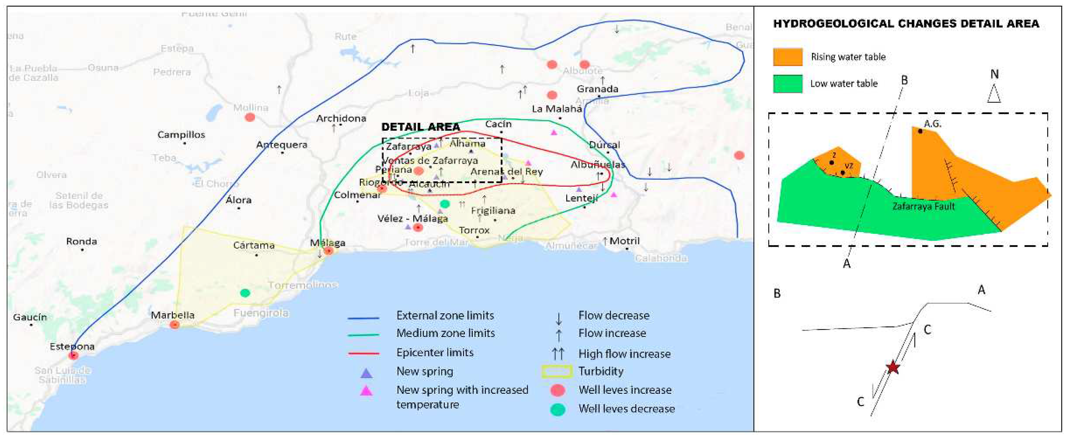
Figure 3.
Left: Geological section of the Zafarraya fault. Right: Detail section of the near-surface region with the filling of the Zafarraya Polje (adapted from [32]).
Figure 3.
Left: Geological section of the Zafarraya fault. Right: Detail section of the near-surface region with the filling of the Zafarraya Polje (adapted from [32]).
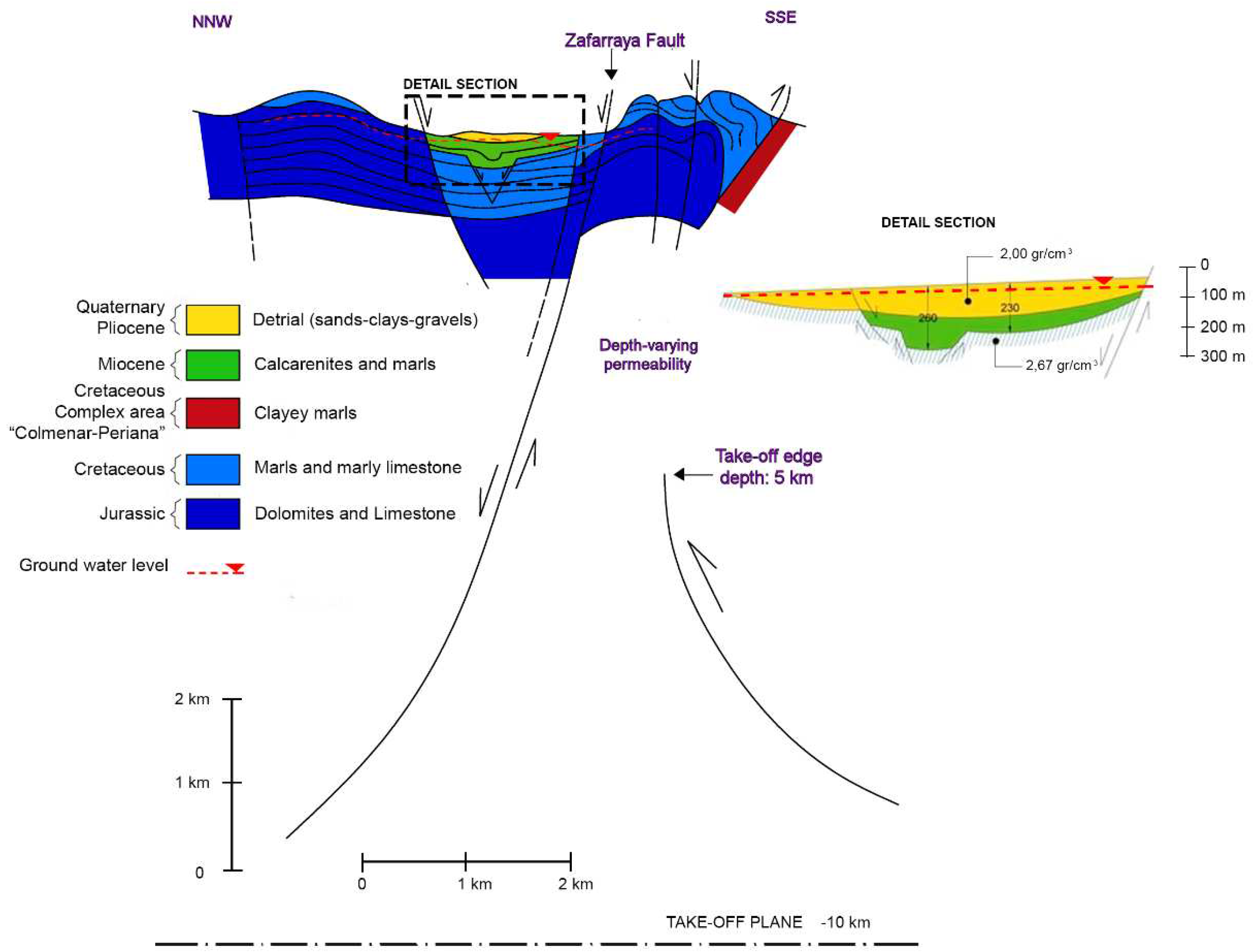
Figure 4.
Schematic flowchart of the hydro-geomechanical coupling of the diverse physics involved in the numerical simulation.
Figure 4.
Schematic flowchart of the hydro-geomechanical coupling of the diverse physics involved in the numerical simulation.
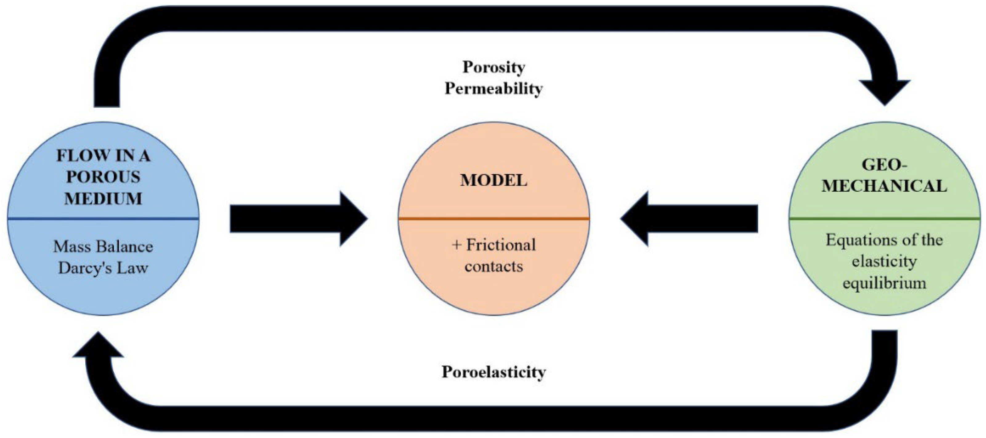
Figure 5.
State of initial stresses (von Mises) (left) and shear stress state at the fault plane (right) at the beginning of the interseismic period. The acting shear stresses (blue) at the highlighted segment are close to the shear strength (green), thus this region is likely to nucleate the earthquake.
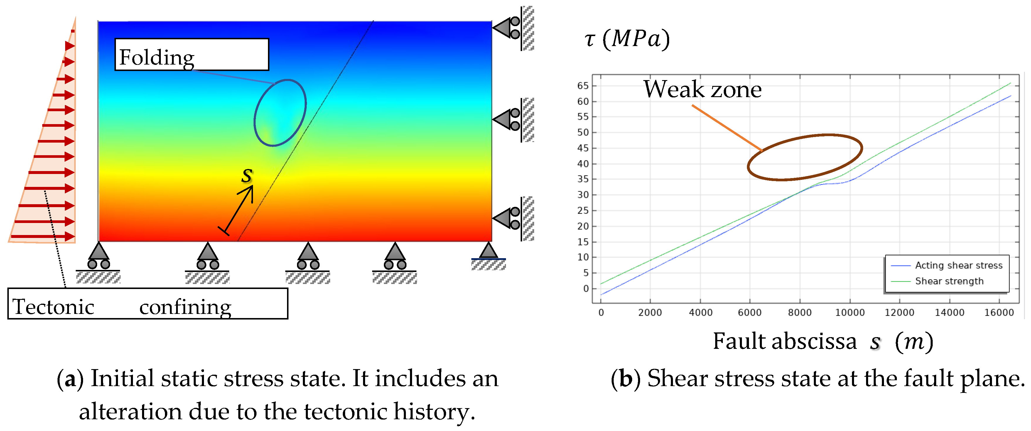
Figure 6.
Hydrostatic pressure field (left) and discretization of the finite element mesh (right).
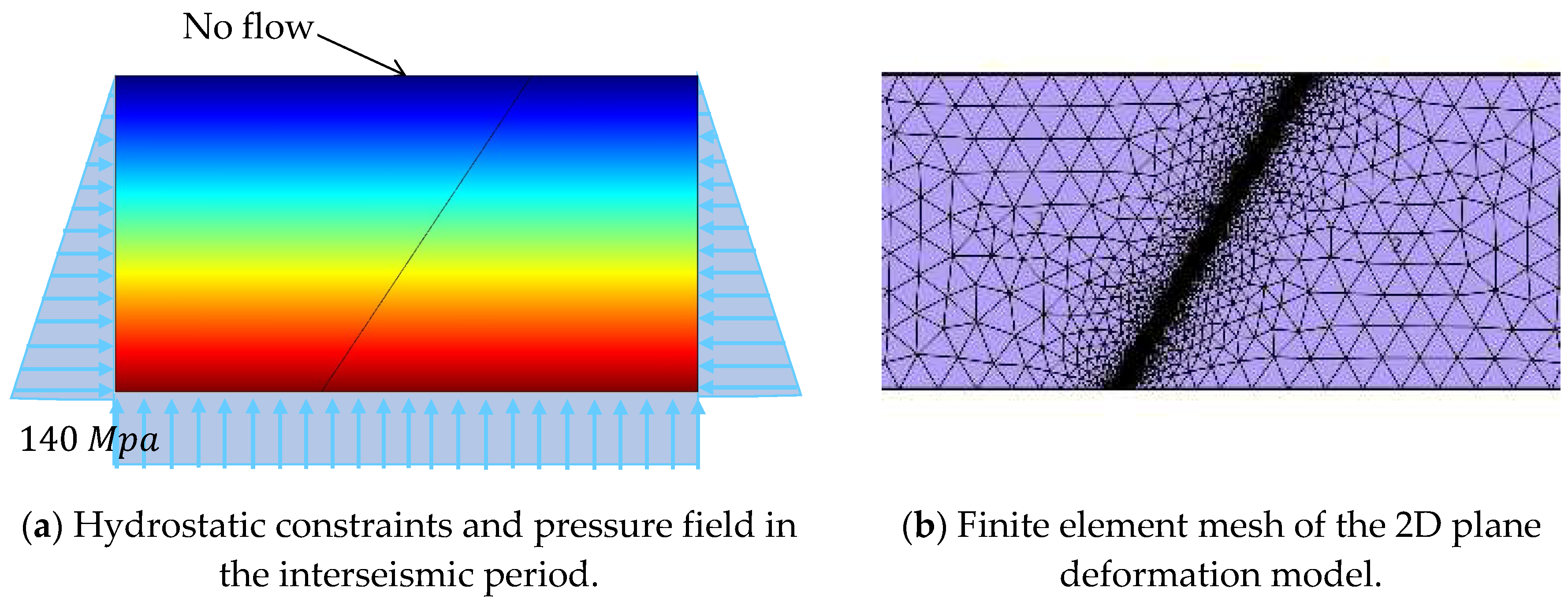
Figure 7.
Results from the dynamic analysis: (a) Total acceleration field (); (b) Maximum pore overpressure () induced by the earthquake.
Figure 7.
Results from the dynamic analysis: (a) Total acceleration field (); (b) Maximum pore overpressure () induced by the earthquake.
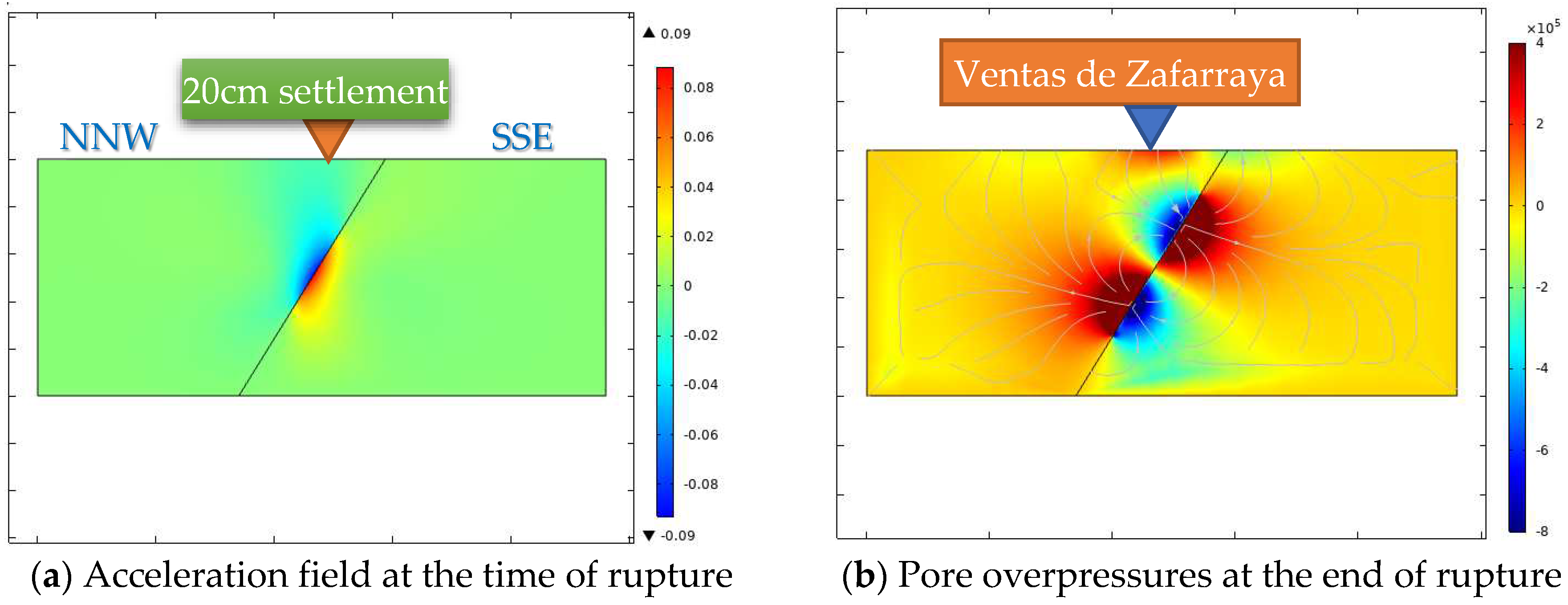
Figure 8.
Time progress of the earthquake rupture: the patch grows in size and accelerates during rupture. Abscissae represent the fault line (m), starting from its bottom. (a) Velocities tangent to the fault plane (). The patch expands as rupture goes on; (b) Relative slip between fault edges (m) induced during the earthquake rupture.
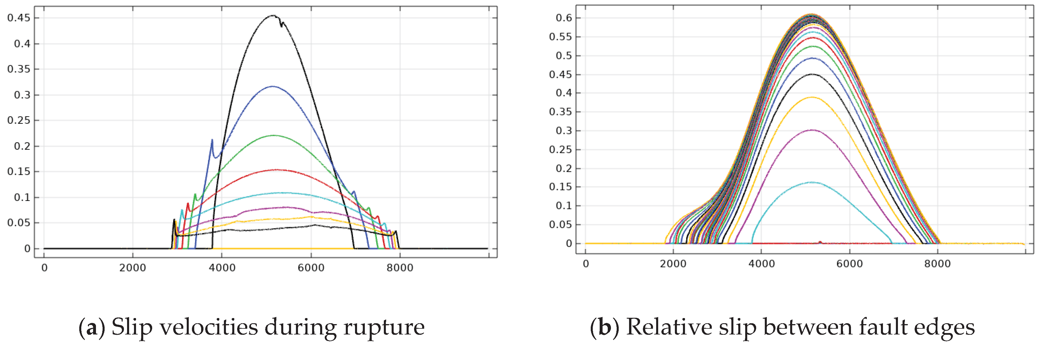

Table 1.
Properties of the ground materials found in the 2D geological model.
| Density (Ton/m3) |
(%) | Permeability (m/s) |
Depth of Water Table (m) |
|
|---|---|---|---|---|
| 1 | 2.00 | 13 | 1 m/day | <15 |
| 2 | 2.00 | 10 | 10-4-10-7 | - |
| 3 | 2.00 | 0.5 | 10-6 | - |
| 4 | - | 0.5 | - | - |
| 5 | 2.67 | 1.5 | 10-3-10-9 | - |
| 6 | 2.67 | 1.5 | 10-3-10-9 | - |
Disclaimer/Publisher’s Note: The statements, opinions and data contained in all publications are solely those of the individual author(s) and contributor(s) and not of MDPI and/or the editor(s). MDPI and/or the editor(s) disclaim responsibility for any injury to people or property resulting from any ideas, methods, instructions or products referred to in the content. |
© 2023 by the authors. Licensee MDPI, Basel, Switzerland. This article is an open access article distributed under the terms and conditions of the Creative Commons Attribution (CC BY) license (https://creativecommons.org/licenses/by/4.0/).
Copyright: This open access article is published under a Creative Commons CC BY 4.0 license, which permit the free download, distribution, and reuse, provided that the author and preprint are cited in any reuse.


