
Submitted:
26 November 2024
Posted:
27 November 2024
You are already at the latest version
Abstract
This study examines the hydrogeological response to seismic activity in the southeastern region of Korea, focusing on groundwater-level changes induced by the 2016 Gyeongju earthquake (ML 5.8). Using a 2D hydro-mechanical coupled bonded particle model, we simulated the dynamic fault rupture process to analyze stress redistribution and its impact on pore pressure and groundwater levels. The results indicate that compressional areas correlate strongly with pore pressure increases and groundwater-level rises, while extensional areas show decreases in both. Observations from the groundwater monitoring well at Gyeongju Cheonbuk, located approximately 10 km north of the earthquake’s epicenter, align well with the model's predictions, providing validation for the simulation. These findings highlight the capability of hydro-mechanical models to capture fault-induced hydrological responses and offer valuable insights into the interplay between seismic activity and groundwater systems.
Keywords:
Gyeongju earthquake
; Fault dynamic rupture
; Groundwater level
; Discrete Element Modelling
1. Introduction
Up to now, many studies have been actively conducted to monitor earthquake induced ground change and earthquake occurrence, using various factors (changes in groundwater level, changes in radon concentration in soil, movement of oil reserves). In particular, changes in groundwater level and groundwater quality that can be quantita-tively measured, have been studied in terms of earthquake monitoring and prediction [1, 2]. Relationship between earthquakes and groundwater levels began to be studied in the 1930s, and with the development of automatic ground-water level measuring devices, many studies have been conducted since the 1970s to clarify the relationship between earthquakes and groundwater levels, and the resulting changes in Earth deformation and stress distribution [3-7].
Many studies have been conducted on groundwater response to earthquakes since groundwater levels are sensitive to changes in stress in the medium [8-13]. Changes in groundwater level due to earthquakes are caused by (1) compression of alluvial deposits [5], (2) undrained expansion and consolidation of saturated sedimentary rocks [14-16], (3) decrease in fluid pressure due to gas outflow from pores [17], (4) changes in permeability within rock mass due to removal of clogging and relaxation of fractures in rock mass caused by fluid movement along the earthquake [18, 19], (5) stress changes in the upper alluvium such as liquefaction [20], and (6) inflow of surface water due to changes in permeability of rock mass.
The precursor of earthquakes has been analyzed based on the changes in groundwa-ter levels and water quality before and after large-scale earthquakes [21-26], and studies on groundwater level fluctuations due to smaller but more frequent intermediate-magnitude earthquakes (e.g., Gyeongju and Pohang earthquakes in Korea) have also been actively conducted [27-30]. Stejskal et al. [30] analyzed the groundwater level fluctuations at the locations of 11.3 km and 16.8 km away from the epicenter of the M2.4 and M3.3 earthquakes, respectively and reported that groundwater level fluctuations due to small-scale earthquakes of magnitude 3.5 or less were observed only on the wells in structurally weak ground. Many studies have also been conducted on groundwater level changes according to distance from the epicenter [31-33] and groundwater quality changes using radon concentration in groundwater [34-44].
Since groundwater levels are sensitive to changes in stress in geological media and have been utilized in earthquake research [8-12]. In the case of the strike-slip fault earthquake that occurred in Iceland in 2000, the groundwater level mainly increased in areas where stress increased, and decreased in areas where stress decreased [45]. However, it can be confirmed that the areas of increased and decreased stress formed after the earthquake showed trends that were opposite to those formed at the co-seismic period of the earthquake. Meanwhile, in the area of increased volumetric strain formed by the displacement of the source fault of the Wenchun earthquake in China, the groundwater level decreased due to the decrease in pore water pressure, and in the area of decreased volumetric strain, the pore water pressure increased due to the compressive force acting on the area, causing the groundwater level to rise [46]. In 2012, in Emilia, Italy, increased and decreased volumetric strain was occurred due to co-seismic displacement [47]. That is, in shallow areas, the volumetric strain increased, causing the pore water pressure to decrease, and the groundwater level tended to decrease; while in areas of deep place, the volumetric strain decreased, causing the pore water pressure to increase, and the groundwater level increased.
The objective of this study is to investigate the relationship between stress redistribution induced by the 2016 Gyeongju earthquake (ML 5.8) and its impact on groundwater-level changes in the southeastern region of Korea.
2. Study Area
2.1. Geological Description
As the objective of the study is to investigate the spatial correlation between the stress changes by the 2016 Gyeongju earthquake and the groundwater level variations monitored at the groundwater level monitoring wells, we focused on the geological setting of the south-east region of Korea as shown in Figure 1. The southeastern part of the Korean Peninsula is mainly composed of Cretaceous sedimentary rocks belonging to the Gyeongsang Supergroup and granite and volcanic rocks (rhyolite, basaltic andesite, and porphyritic dacite) that intruded the sedimentary rocks in Tertiary. The sedimentary rocks are mainly composed of shale and sandstone, and are mostly hornfelsic. The granite rocks are mainly composed of medium-grained granodiorite and medium- to fine-grained biotite granite, and are distributed in the northeastern part of the study area. In addition, feldspathic porphyry is distributed. In the southeastern part of the Korean Peninsula, the Yangsan fault is developed in the NE-SSE direction, and the Ulsan fault is developed in the NE-SSE direction. In addition, the Miryang, Moryang, Dongrae, and Ilgwang faults are distributed (Figure 1.).
2.2. Groundwater Level Monitoring Wells and Level Changes Induced by the 2016 Gyeongju Earthquake
We analyzed the correlation between pore pressure change and the groundwater level change induced by the 2016 Gyeongju earthquake. Figure 2 visualizes the groundwater level changes at monitoring wells in response to the 2016 Gyeongju earthquake. Each triangle represents the locations of groundwater monitoring wells distribute in the south-east region of Korea. The level changes are shown by upward-pointing triangles indicating wells where the groundwater level rose, and downward-pointing triangles indicating wells where the groundwater level dropped. The color gradient conveys the magnitude of change: dark red represents a significant groundwater level rise, light red indicates a smaller rise, and dark to light blue represents varying degrees of groundwater level drop. The distribution of these changes is closely tied to the stress redistribution caused by the right-lateral strike-slip fault motion. Wells showing significant groundwater level rises (dark red triangles) are predominantly located in regions where the stress increased due to the compressional effects of the fault slip. The compressional stress caused by the right-lateral strike-slip faulting compresses the pore spaces in the aquifer, increasing pore pressure and leading to a groundwater level rise. This spatial correlation between groundwater level rise and stress increase highlights the direct influence of fault mechanics on subsurface hydrological responses. In contrast, wells experiencing groundwater level drops (blue triangles) are situated in regions of stress decrease caused by extensional effects of the fault slip. Here, the reduced stress results in an expansion of pore spaces, lowering pore pressure and causing a groundwater level drop.
3. Methods
3.1. Hydro-Mechanical Coupling Concept in PFC2D
In order to simulate pore pressure variations induced by the dynamic geomechanical processes, i.e., fault dynamic rupture, which is a hydro-mechanical coupled processes, we developed a pore-pipe network model and implemented in the 2D particle assembly. Figure 3a shows the 2D version of the pore-pipe network model. The blue polygons are the fluid domains constructed by lines linked to adjacent particles at their centers. The short red lines are the pipes for fluid flow based on Darcy’s law and Poiseuille equation, which assumes fluid from one domain to a nearby one in the form of laminar flow. Each cycle of hydro-mechanical coupling in the pipe network model can be divided into three steps. Firstly, the volumetric flow rate in each pipe is calculated by the hydraulic aperture and fluid pressure gradient. Secondly, the fluid pressure in each fluid domain is updated considering the fluid volume increment. Lastly, the fluid pressure is exerted on solid particles by an additional force, as in Figure 3b. The mathematical formulation of the pore-pipe network model is based on finite volume method which can be referred to in [49].
Figure 4 presents the calculation steps of the hydro-mechanical coupling processes. In this figure, the left part is the DEM modeling in PFC2D for the solid deformation and movement, while the right part, is the fluid flow modeling based on FVM. FVM for fluid flow has two steps: constructing a linear system based on the continuity equation of a Stokes flow in each fluid domain and solving the linear system in Python to obtain pore pressure field. During the coupling process, the local conductance of each pipe and the volume increment of each fluid domain are calculated from the DEM particle system. The pore pressure includes the hydrostatic pressure and the losses of piezometric pressure due to fluid flow.
3.2. Dynamic Fault Rupture Modelling in PFC2D
Figure 5 describes the workflow of the dynamic fault rupture simulation. This workflow outlines the process for simulating dynamic fault rupture using PFC. The workflow begins with the creation of an unbonded particle assembly, where particles are densely packed within the study domain. The study area domain is 120 km x 180 km in size, and densely packed with the particle of which radii ranged from 200–300 m. In total, 93318 particles were used. The particles are then bonded at their contacts, which mimics the cohesive properties of rockmass and faults. Faults are then inserted into the model (Figure 6), along with their properties, using the smooth joint contact model [50] to represent the mechanical behavior of fault planes. This is followed fault dynamic rupture process. We used the “lock and release” approach [51]. In this approach, a finite length of the fault at the hypocenter location was locked. After that, the entire model domain was initialized uniformly with the in-situ stress model, which is representative for the south-east region of Korea (Figure 7a) [52]. The maximum horizontal stress orientation prevalent in the south-east region of Korea is N70E (Figure 7b) [53]. The stress initialization was done by the PFC2D command “BALL TRACTION”, so that the maximum stress is in the orientation of N70E throughout the entire model domain as shown by the stress tensors in Figure 6. A quiet boundary condition is set to the boundaries to minimize the seismic wave reflecting back to the model. It is to mimic a semi-infinite space. Then the pore-pipe network model is introduced, and pore pressure is initialized uniformly throughout the entire model domain. A fault dynamic rupture is then simulated by instantaneously unlocking the previously locked part of the fault. A locking radius of 1400 m, corresponding to a fault length of 2800 m, was applied. The rupturing fault trace size was calibrated based on fault scaling relations introduced in [54], to result in an event moment magnitude consistent with that of the 2016 Gyeongju mainshock. Upon fault unlocking, the strain energy previously stored along the locked fault trace is released and results in seismic wave initiation and propagation (Figure 8). Due to damping of the particles, the seismic wave attenuates as it propagated. During this process, the pore volume changes due to mechanical stress effect and pore pressure changes occurs due to poro-elasticity effect. Pore pressure evolutions at several selected locations are recorded to analyze their evolutions over time. The model is then run for 100 seconds to simulate the dynamic rupture process, capturing the fault’s mechanical and hydraulic responses.
4. Results
4.1. Coseismic Displacement Distribution
Figure 9 illustrates the particle displacement vectors at 30 seconds after the start of the simulation, demonstrating the deformation caused by the fault rupture during the 2016 Gyeongju earthquake. The vector arrows represent the magnitude and direction of particle displacement, while the color scale provides a quantitative measure of displacement, with warmer colors (e.g., red and orange) indicating higher magnitudes and cooler colors (e.g., blue) representing lower magnitudes.
The pattern of the displacement vectors shows a right-lateral slip, which is consistent with the observed faulting mechanism of the 2016 Gyeongju earthquake and consistent with the results of several other studies, e.g., [55]. This right-lateral motion aligns with the seismic moment tensor solutions for the event, confirming that the simulation well represents the fault dynamics. The displacement is concentrated along the fault plane, with the largest vectors located near the fault center, indicating the primary zone of rupture and slip.
4.2. Spatial and Temporal Evolution of Pore Pressure
Figure 10 illustrates the pore pressure evolution at 5, 10, and 15 seconds following the initiation of fault dynamic rupture. The high pore pressure zones align closely with areas of stress increase caused by the right-lateral fault slip, emphasizing the strong coupling between fault mechanics and pore fluid behavior during seismic events. At 5 seconds, the pore pressure response is highly localized around the fault rupture zone. The highest pore pressure regions (indicated by red and orange) are concentrated along the fault traces where the stress increases due to the right-lateral fault slip. This localized pressure rise reflects the immediate transfer of stress changes into the pore space. The right-lateral motion causes compressional stresses on one side of the fault and extensional stresses on the other, and the high pore pressure zones correspond to the compressional side where the stress increases the most. This finding seems consistent with the interpretation of groundwater level rise and drop cause by the 2009 Wenchuan earthquake [46]. By 10 seconds, the high-pressure regions expand outward from the fault, following the spatial distribution of stress increases caused by the fault motion. The propagation of pore pressure changes is influenced by the fault’s slip mechanics, with the most significant increases remaining aligned with areas of high compressional stress. This shows that the pore pressure response is not uniform but strongly tied to the stress perturbations induced by the fault slip. At 15 seconds, the high pore pressure zones continue to expand but remain concentrated near regions of maximum stress increase. These zones still align with areas affected by the right-lateral slip dynamics, particularly where compressional forces dominate. While the pressure gradients start to stabilize and diffuse into the surrounding medium, the sustained high-pressure regions near the fault emphasize the prolonged impact of stress-induced pore pressure changes.
4.3. Correlation Between Pore Pressure and Groundwater Level Evolution
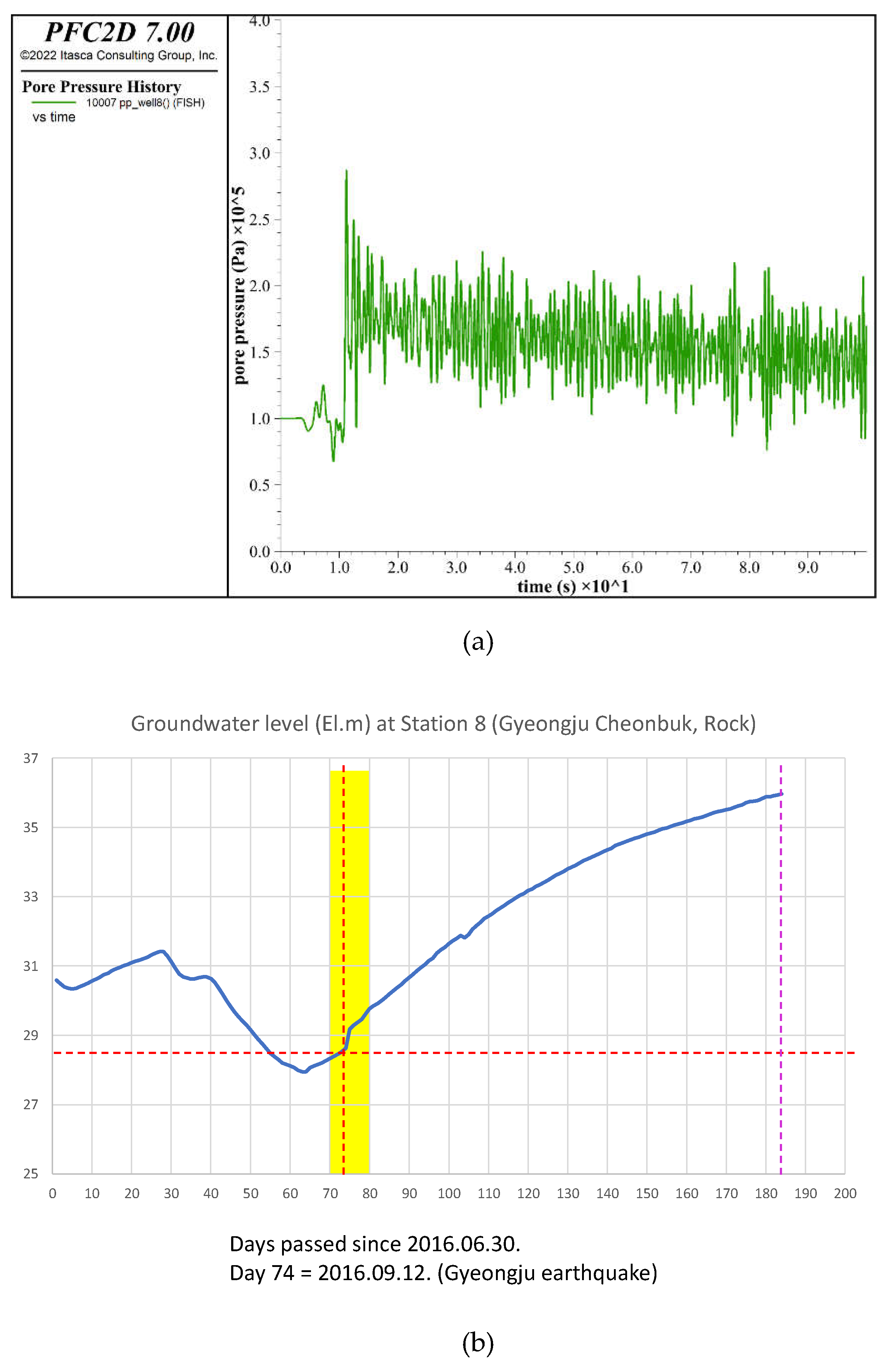
Figure 11 provides insights into the response of pore pressure and groundwater levels at Well 8 (Gyeongju Cheonbuk) following the 2016 Gyeongju earthquake. Figure 11a shows the simulated pore pressure history at Well 8, derived from a PFC2D model. The pore pressure exhibits an instantaneous and sharp rise at the moment of the earthquake, representing the rapid stress transfer caused by the fault rupture. After this abrupt increase, the pressure undergoes a slow decay phase, reflecting the gradual dissipation of excess pressure as the system approaches equilibrium. Despite the decline in the rate of increase, the pressure remains consistently positive, indicating that the pore pressure in the aquifer stabilizes at a higher level compared to its initial state. This behavior highlights the persistent impact of the earthquake on the subsurface hydrology in the near field.
Figure 11b displays the observed groundwater level changes at Well 8 Gyeongju Cheonbuk. At the onset of the earthquake, there is a sharp rise in groundwater levels, which closely correspond to the simulated instantaneous pore pressure increase seen in Figure 9a. Following the initial spike, the groundwater level continues to rise gradually, indicating a slower, sustained upward trend. This steady increase aligns with the simulated decay phase of the pore pressure, demonstrating how the hydrological system adjusts over time to the stress changes induced by the fault rupture. The leveling-off of the rise reflects the decreasing rate of pressure increase, as observed in the simulated data.
The relationship between the two figures underscores the strong correlation between pore pressure and groundwater level responses. The instantaneous rise in pore pressure drives the sharp groundwater level increase, while the slower decay in pressure explains the gradual leveling-off of groundwater level changes. Importantly, the consistent positive pressure in the simulation translates to a sustained upward trend in groundwater levels, confirming that the fault rupture caused a lasting hydrological effect in the near field.
5. Conclusions
The groundwater system’s response to the 2016 Gyeongju earthquake highlights the intricate interplay between fault mechanics and subsurface hydrology. The analysis of groundwater level changes, pore pressure evolution, and stress redistribution provides critical insights into the mechanisms driving hydrological responses during seismic events.
The spatial distribution of groundwater level rises and drops, as observed at the monitoring wells, aligns strongly with the stress redistribution caused by the right-lateral strike-slip faulting. Wells experiencing significant groundwater level rises are predominantly located in regions where stress increased due to compressional effects, while groundwater level drops correspond to areas of stress reduction caused by extensional effects. This correlation underscores the strong coupling between fault mechanics and pore pressure changes, demonstrating how seismic stress redistributes and influences the behavior of groundwater systems.
Simulations of pore pressure evolution further validate these observations. High pore pressure zones were shown to concentrate in regions of stress increase near the fault, propagating outward with time. The modeled dynamics, including an initial sharp pressure rise followed by a slower decay, effectively capture the transient and persistent nature of groundwater level changes observed in the near field. The model demonstrates its capability to accurately reproduce the physics of fault-induced stress redistribution and its hydrological consequences, capturing both the immediate and long-term groundwater responses to seismic activity.
However, while the model performs well in reproducing near-field observations, its performance in the far field is less satisfactory. The far-field groundwater level changes are likely influenced by local geological factors, such as aquifer heterogeneity, permeability variations, and fault connectivity, which are not fully captured in the model. These localized effects introduce variability that complicates the correlation between modeled stress redistribution and observed hydrological responses in the far field.
Hence, the integrated analysis of observational data and simulations provides a robust framework for understanding earthquake-induced groundwater system behavior. The model’s ability to capture the underlying physical processes driving stress and pore pressure changes offers confidence in its application to study similar seismic events. While the near-field groundwater level responses are well simulated, the limitations in far-field simulations highlight the need to account for local geological variability in future modeling efforts. The correlation between stress redistribution, pore pressure evolution, and groundwater level changes underscores the utility of these approaches for studying the hydrological impacts of seismic events and advancing our understanding of fault-hydrology interactions.
Supplementary Materials
The following supporting information can be downloaded at: Preprints.org, Figure S1: title; Table S1: title; Video S1: title.
Author Contributions
Conceptualization, H.C. and S.Y.H.; Methodology, H.C. and J.S.Y.; Software, J.S.Y.; Validation, H.C., J.S.Y., S.G.K. and J.Y.C.; Investigation, H.C.; Resources, J.S.Y.; Data curation, S.G.K.; Writing—original draft preparation, H.C.; writing—review and editing, J.S.Y. and J.Y.C; Visualization, H.C.; Supervision, J.S.Y., J.Y.C. and S.Y.H.; Project administration, S.G.K. and J.Y.C.; Funding acquisition, S.G.K. and J.Y.C. All authors have read and agreed to the published version of the manuscript.
Funding
This research was funded by the Korea Institute of Energy Technology Evaluation and Planning (KETEP) grant funded by the Korea government Ministry of Trade, Industry and Energy (Project Number: RS-2023-00236697).
Informed Consent Statement
Informed consent was obtained from all subjects involved in the study.
Data Availability Statement
De-identified data can be made available upon request to the corresponding author and permission granted from subjects involved in this study in release of their data.
Conflicts of Interest
The authors declare no conflicts of interest.
References
- Chen, A.T.; Ouchi, T.; Lin, A.; Chen, J.; Maruyama, T. Phenomena Associated with the 1999 Chi-Chi Earthquake in Taiwan, Possible Precursors and After Effects. Terr. Atmospheric Ocean. Sci. 2000, 11, . [CrossRef]
- Che, Y. T., Zhao, W. Z., Yu, J. Z., and Liu, C. L., 2006, Digitalized well-water-level observation and monitoring efficiency evaluation of earthquake precursor in the Beijing-Tianjin-Hebei region, Earthquake, 26(4).
- Leggette, R.M.; Taylor, G.H. Earthquakes instrumentally recorded in artesian wells*. Bull. Seism. Soc. Am. 1935, 25, 169–175, . [CrossRef]
- Bower, D. R., and Heaton, K. C., 1978, Response of an aquifer near ottawa to tidal forcing and the alaskan eqrthquak of 1964., Can J Earth Sci, 15(3). [CrossRef]
- Roeloffs, E.A. Persistent water level changes in a well near Parkfield, California, due to local and distant earthquakes. J. Geophys. Res. 1998, 103, 869–889, . [CrossRef]
- King, C. Y., Azuma, S., Igarashi, G., Ohno, M., Saito, H., and Wakita, H., 1999, Earthquake-related water-level changes at 16 closely clustered wells in Tono, central Japan, Journal of Geophysical Research: Solid Earth, 104(B6). [CrossRef]
- Cicerone, R.D.; Ebel, J.E.; Britton, J. A systematic compilation of earthquake precursors. Tectonophysics 2009, 476, 371–396, . [CrossRef]
- Merifield, P.M.; Lamar, D.L. Possible strain events reflected in water levels in wells along San Jacinto fault zone, southern California. Pure Appl. Geophys. 1985, 122, 245–254, . [CrossRef]
- Rojstaczer, S.; Agnew, D.C. The influence of formation material properties on the response of water levels in wells to Earth tides and atmospheric loading. J. Geophys. Res. 1989, 94, 12403–12411, . [CrossRef]
- Roeloffs, E.A. Hydrologic precursors to earthquakes: A review. Pure Appl. Geophys. 1988, 126, 177–209, . [CrossRef]
- Roeloffs, E.; Quilty, E.; Scholtz, C.H. Case 21 water level and strain changes preceding and following the August 4, 1985 Kettleman Hills, California, earthquake. Pure Appl. Geophys. 1997, 149, 21–60, . [CrossRef]
- Kitagawa, Y.; Koizumi, N.; Takahashi, M.; Matsumoto, N.; Sato, T. Changes in groundwater levels or pressures associated with the 2004 earthquake off the west coast of northern Sumatra (M9.0). Earth, Planets Space 2006, 58, 173–179, . [CrossRef]
- Shi Z., Wang G., and Liu C., 2014, Advances in research on earthquake fluids hydrogeology in China: a review, Earthquake, Sci., 26(6), 415-425. [CrossRef]
- Wang, C.-Y.; Cheng, L.-H.; Chin, C.-V.; Yu, S.-B. Coseismic hydrologic response of an alluvial fan to the 1999 Chi-Chi earthquake, Taiwan. Geology 2001, 29, . [CrossRef]
- Manga, M.; Brodsky, E.E.; Boone, M. Response of streamflow to multiple earthquakes. Geophys. Res. Lett. 2003, 30, . [CrossRef]
- Wang, C.; Chia, Y. Mechanism of water level changes during earthquakes: Near field versus intermediate field. Geophys. Res. Lett. 2008, 35, . [CrossRef]
- Matsumoto, N.; Roeloffs, E.A. Hydrological response to earthquakes in the Haibara well, central Japan—II. Possible mechanism inferred from time-varying hydraulic properties. Geophys. J. Int. 2003, 155, 899–913, . [CrossRef]
- Brodsky, E.E.; Roeloffs, E.; Woodcock, D.; Gall, I.; Manga, M. A mechanism for sustained groundwater pressure changes induced by distant earthquakes. J. Geophys. Res. 2003, 108, . [CrossRef]
- Koizumi, N., Lai, W. C., Kitagawa, Y., and Matsumoto, N., 2004, Comment on “Coseismic hydrological changes associated with dislocation of the September 21, 1999 Chichi earthquake, Taiwan” by Min Lee et al., Geophysical Research Letters, 31(13). [CrossRef]
- Wang, C. Y., and Manga, M., 2014, Earthquakes and Water, Encyclopedia of Complexity and Systems Science, Springer Science + Business Media New York 2014.
- Che, Y. T., and Yu J. Z., 1992, Preliminary approach to quality-evaluation method of seismo- groundwater observation wells, Earthquake (Beijing), 1(1).
- Che, Y. T., Yu, J. Z., Zhang, D., Sun, Z. A., Jian, C. L., and Peng, G., 1994, Annual regime characteristics of water level in bedrock wells in Beijing plain, Seismology & Geology, 16(3).
- Geng, J., Zhang, Z., Wei, H., and Wang, Z., 1998, Dynamic pattern of groundwater level before and after the Tangshan earthquake and its mode of formation and evolution, Dizhen Dizhi, 20(3).
- Liu, C., Wang, G., Zhang, W., and Mei, J., 2009, Coseismic responses of groundwater levels in the Three Gorges well-network to the Wenchuan M S8.0 earthquake, Earthquake Science, 22(2).
- Wang, W. X., Shi, Y. L., Zhang, J., and Shi, Y. H., 2009, Dynamic gravity changes before and after the 2006 wen’an M5.1 earthquake, hebei province, Earthquake, 29(2).
- Yin, X. C., Zhang, L. P., Zhang, Y. X., Pang, K. Y., Wang, H. T., Song, Z. P., and Yuan, S., 2009, Large scale LURR anomaly before wenchuan earthquake, Earthquake, 29(1).
- Sun Z. A., Sun T., and Wang Y., 1997, Anomalous features of ground water behaviour in Banqiao well around the Shunyi earthquake with Ms 4.0, Beijing, Earthquake (Beijing), 17(4).
- Ma, J. Y., Liu, X. L., and Li, J. Y., 2008, Anomaly characteristics of subsurface fluid in Tianjin region before Wen’an earthquake with Ms5.1, Earthquake, 28(1).
- Ramana, D.V.; Chadha, R.K.; Singh, C.; Shekar, M. Water level fluctuations due to earthquakes in Koyna-Warna region, India. Nat. Hazards 2006, 40, 585–592, . [CrossRef]
- Stejskal, V.; Kašpárek, L.; Kopylova, G.N.; Lyubushin, A.A.; Skalský, L. Precursory groundwater level changes in the period of activation of the weak intraplate seismic activity on the NE margin of the Bohemian Massif (central Europe) in 2005. Stud. Geophys. et Geod. 2009, 53, 215–238, . [CrossRef]
- Roeloffs, E.; Sneed, M.; Galloway, D.L.; Sorey, M.L.; Farrar, C.D.; Howle, J.F.; Hughes, J. Water-level changes induced by local and distant earthquakes at Long Valley caldera, California. J. Volcanol. Geotherm. Res. 2003, 127, 269–303, . [CrossRef]
- Liu, C.; Huang, M.-W.; Tsai, Y.-B. Water Level Fluctuations Induced by Ground Motions of Local and Teleseismic Earthquakes at Two Wells in Hualien, Eastern Taiwan. Terr. Atmospheric Ocean. Sci. 2006, 17, . [CrossRef]
- Chadha, R.; Kuempel, H.-J.; Shekar, M. Reservoir Triggered Seismicity (RTS) and well water level response in the Koyna–Warna region, India. Tectonophysics 2008, 456, 94–102, . [CrossRef]
- Wakita, H.; Nakamura, Y.; Notsu, K.; Noguchi, M.; Asada, T. Radon Anomaly: A Possible Precursor of the 1978 Izu-Oshima-kinkai Earthquake. Science 1980, 207, 882–883, . [CrossRef]
- Wakita, H.; Igarashi, G.; Nakamura, Y.; Sano, Y.; Notsu, K. Coseismic radon changes in groundwater. Geophys. Res. Lett. 1989, 16, 417–420, . [CrossRef]
- Ramola, R. C., Singh, M., Sandhu, A. S., Singh, S., and Virk, H. S., 1990, The use of radon as an earthquake precursor, Nuclear Geophysics, 4(2).
- Wakita, H.; Igarashi, G.; Notsu, K. An anomalous radon decrease in groundwater prior to an M6.0 earthquake: A possible precursor?. Geophys. Res. Lett. 1991, 18, 629–632, . [CrossRef]
- Monnin, M.; Seidel, J. Radon in soil-air and in groundwater related to major geophysical events: A survey. Nucl. Instruments Methods Phys. Res. Sect. A: Accel. Spectrometers, Detect. Assoc. Equip. 1992, 314, 316–330, . [CrossRef]
- Plastino, W., Bella, F., Catalano, P. G., and Di Giovambattista, R., 2002, Radon groundwater anomalies related to the Umbria-Marche September 26, 1997, earthquakes, Geofisica Internacional, 41(4).
- Yasuoka, Y.; Ishii, T.; Tokonami, S.; Ishikawa, T.; Narazaki, Y.; Shinogi, M. Radon anomaly related to the 1995 Kobe earthquake in Japan. Int. Congr. Ser. 2005, 1276, 426–427, . [CrossRef]
- Miklavčić, I.; Radolić, V.; Vuković, B.; Poje, M.; Varga, M.; Stanić, D.; Planinić, J. Radon anomaly in soil gas as an earthquake precursor. Appl. Radiat. Isot. 2008, 66, 1459–1466, . [CrossRef]
- Ramola, R.; Prasad, Y.; Prasad, G.; Kumar, S.; Choubey, V. Soil-gas radon as seismotectonic indicator in Garhwal Himalaya. Appl. Radiat. Isot. 2008, 66, 1523–1530, . [CrossRef]
- Kuo, T., Lin, C., Fan, K., Chang, G., Lewis, C., Han, Y., Wu, Y., Chen, W., and Tsai, C., 2009, Radon anomalies precursory to the 2003 Mw = 6.8 Chengkung and 2006 Mw = 6.1 Taitung earthquakes in Taiwan, Radiation Measurements, 44(3).
- Ramola, R.C. Relation between spring water radon anomalies and seismic activity in Garhwal Himalaya. Acta Geophys. 2010, 58, 814–827, . [CrossRef]
- Jónsson, S.; Segall, P.; Pedersen, R.; Björnsson, G. Post-earthquake ground movements correlated to pore-pressure transients. Nature 2003, 424, 179–183, . [CrossRef]
- Shi, Z., Wang, G., Manga, M., and Wang, C. Y., 2015, Continental-scale water-level response to a large earthquake, Geofluids, 15(1–2).
- Nespoli, M.; Todesco, M.; Serpelloni, E.; Belardinelli, M.E.; Bonafede, M.; Marcaccio, M.; Rinaldi, A.P.; Anderlini, L.; Gualandi, A. Modeling earthquake effects on groundwater levels: evidences from the 2012 Emilia earthquake (Italy). Geofluids 2015, 16, 452–463, . [CrossRef]
- Kim, G.-B.; Choi, M.-R.; Lee, C.-J.; Shin, S.-H.; Kim, H.-J. Characteristics of spatio-temporal distribution of groundwater level’s change after 2016 Gyeong-ju earthquake. J. Geol. Soc. Korea 2018, 54, 93–105, . [CrossRef]
- Yoon, J.S., and Zhou, J., 2020, Modelling of Fault Deformation Induced by Fluid Injection using Hydro-Mechanical Coupled 3D Particle Flow Code: DECOVALEX-2019 Task B, Tunnel & Underground Space, 30(4), 320-334.
- Mas Ivars, D.; Pierce, M.E.; Darcel, C.; Reyes-Montes, J.; Potyondy, D.O.; Paul Young, R.; Cundall, P.A. The synthetic rock mass approach for jointed rock mass modelling. Int. J. Rock Mech. Min. Sci. 2011, 48, 219–244, doi:10.1016/j.ijrmms.2010.11.014.
- Yoon, J.S.; Stephansson, O.; Zang, A.; Min, K.-B.; Lanaro, F. Discrete bonded particle modelling of fault activation near a nuclear waste repository site and comparison to static rupture earthquake scaling laws. Int. J. Rock Mech. Min. Sci. Géoméch. Abstr. 2017, 98, 1–9, . [CrossRef]
- Kim, H., Synn, J.H., Park, C., Song, W.K., Park, E.S., Jung, Y.B., Cheon, D.S., Bae, S., Choi, S.O., Chang, C., Min, K.B., 2021, Korea Stress Map 2020 using Hydraulic Fracturing and Overcoring Data, Tunnel & Underground Space, 31(3), 145-166.
- Kang, M.; Chang, C.; Bae, S.; Park, C. Spatial variation of in situ stress at shallow depth in South Korea. Geosci. J. 2023, 27, 321–335, . [CrossRef]
- Well, D.L., Coppersmith, K.J., 1994, New empirical relationships among magnitude, rupture length, rupture width, rupture area, and surface displacement, B Seismol Soc Am, 84, 974-1002.
- Uchide, T.; Song, S.G. Fault Rupture Model of the 2016 Gyeongju, South Korea, Earthquake and Its Implication for the Underground Fault System. Geophys. Res. Lett. 2018, 45, 2257–2264, . [CrossRef]
Figure 1.
Geological and faults map of the study area (modified from [48]).
Figure 1.
Geological and faults map of the study area (modified from [48]).
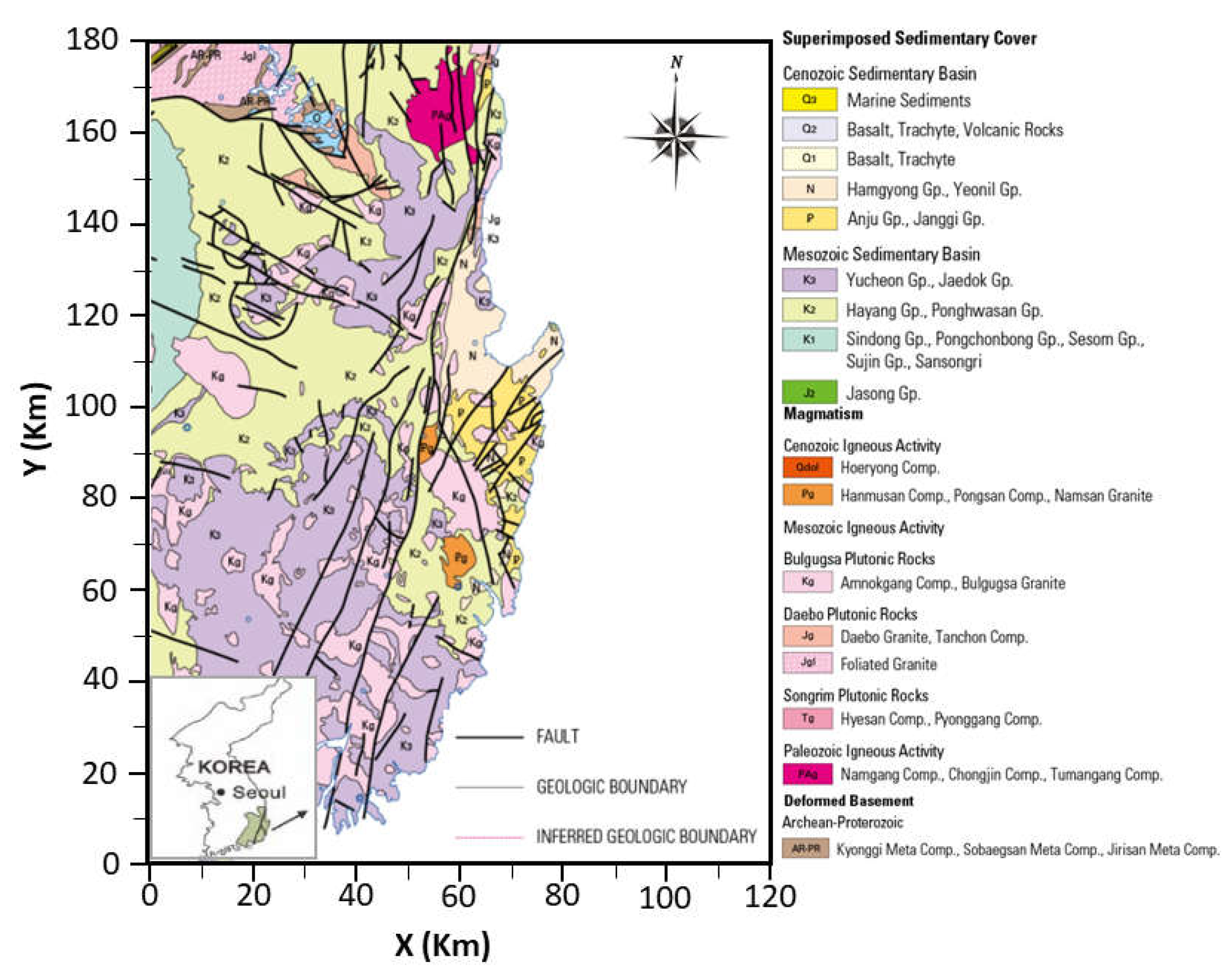
Figure 2.
Locations of groundwater level monitoring wells distributed in the south-east region of Korea. The groundwater level changes monitored at the wells induced by the 2016 Gyeongju earthquake is represented by upward red triangles (level rise) and downward blue triangles (level drop), and the amount of level rise and drop is depicted by the color. The black star is the location of 2016 Gyeongju earthquake. The location with asterisk (*) is Well No. 8 Gyeongju Cheonbuk.
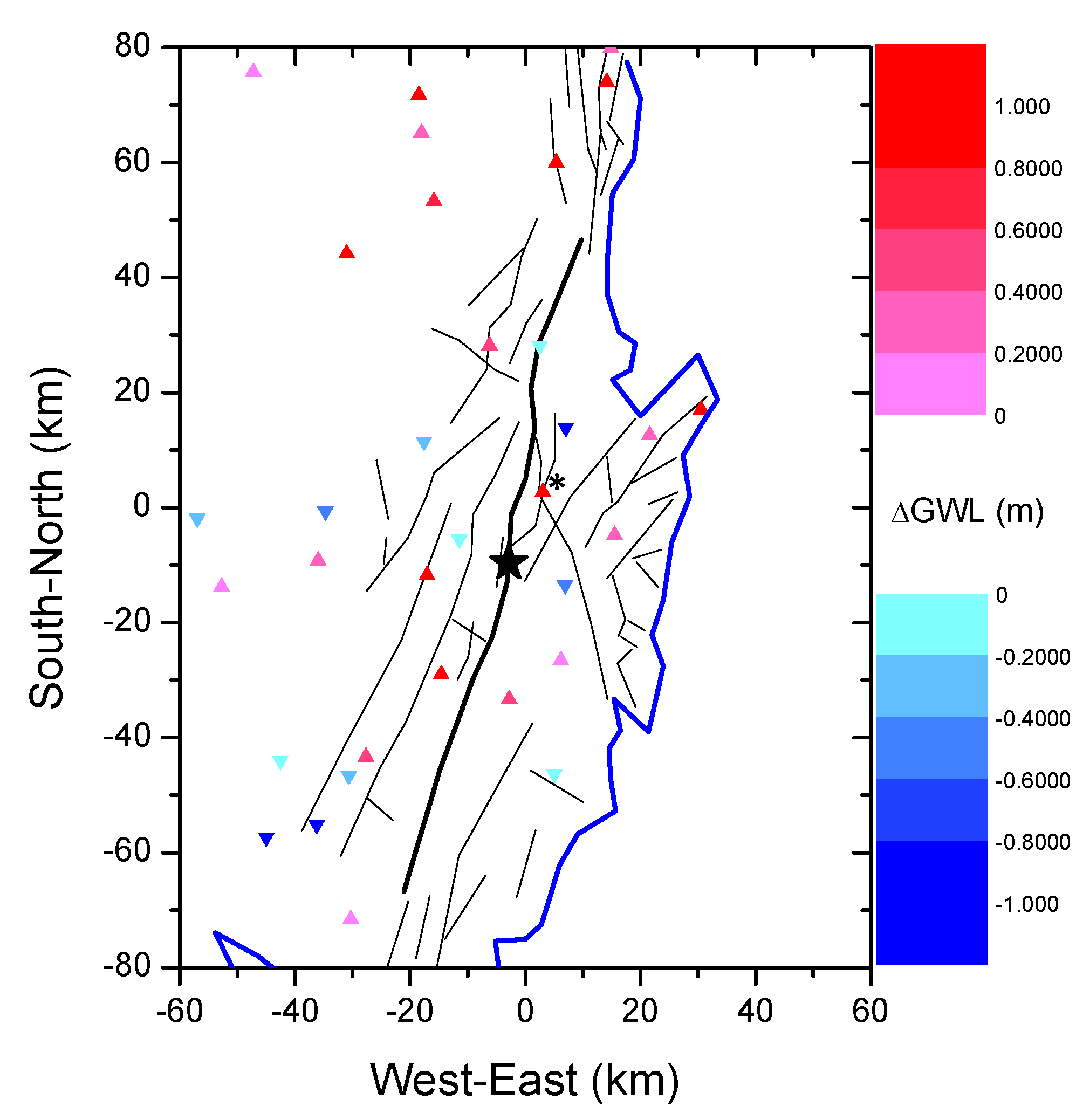
Figure 3.
Workflow for dynamic rupture simulation using PFC.
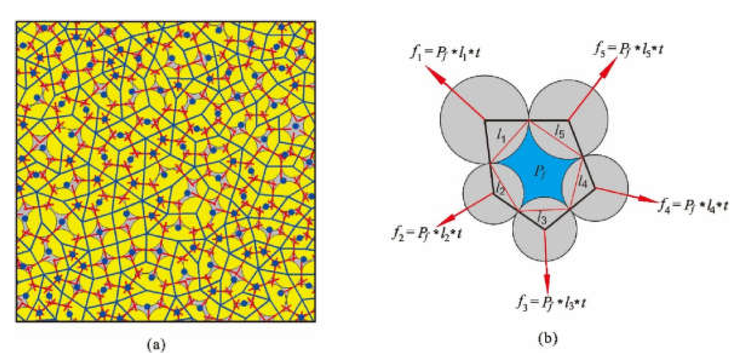
Figure 4.
Calculation steps of the hydro-mechanical coupling processes.
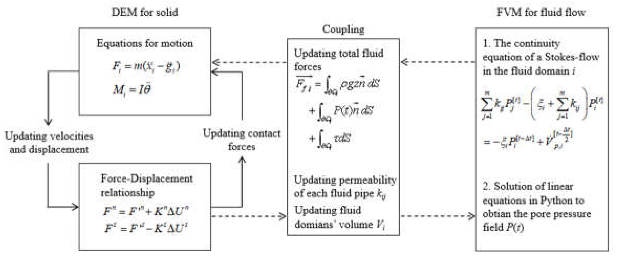
Figure 5.
Workflow for dynamic rupture simulation using PFC.
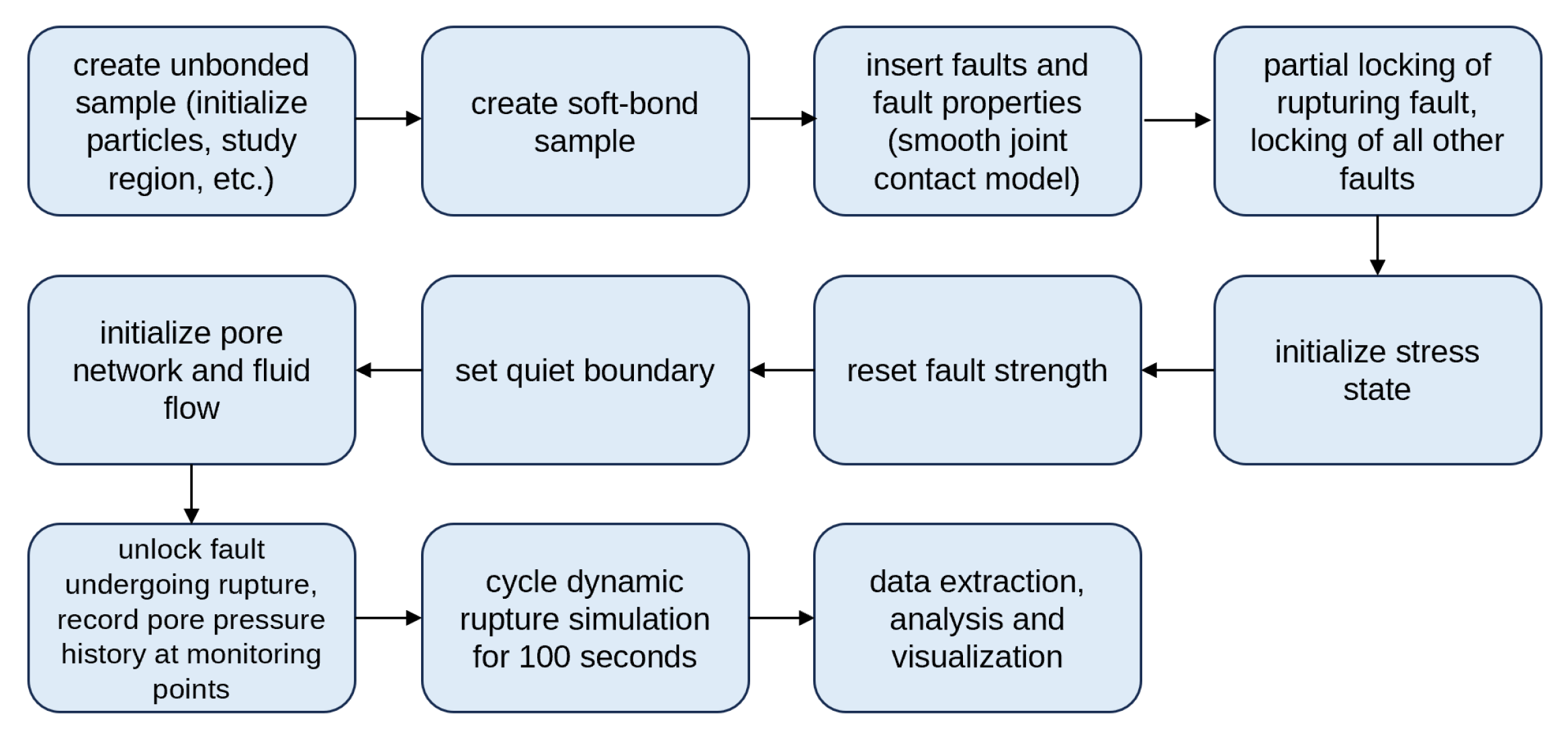
Figure 6.
Faults represented by smooth joint contact model and the orientations of the in-situ horizontal stresses shown by the stress tensor.
Figure 6.
Faults represented by smooth joint contact model and the orientations of the in-situ horizontal stresses shown by the stress tensor.
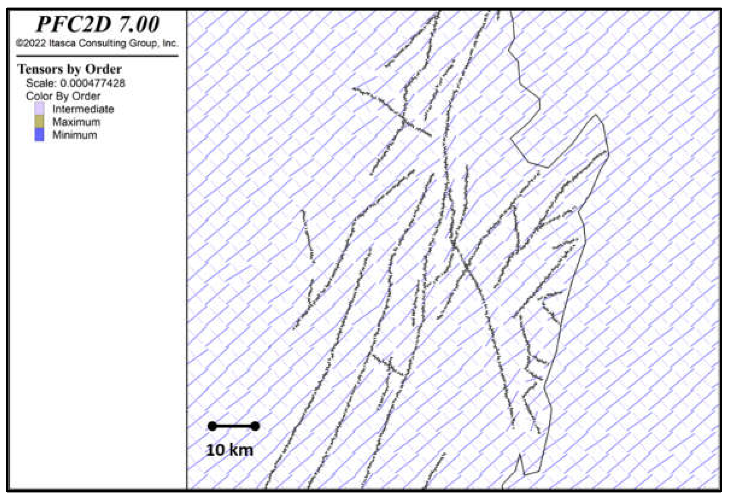
Figure 7.
In-situ stress model of South-East region of Korea [52], and the orientation of the maximum horizontal stress in the region [53].
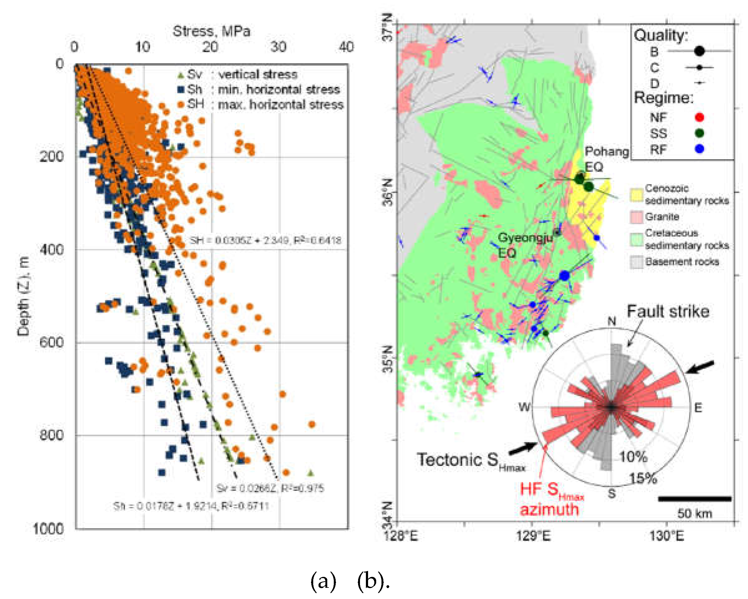
Figure 8.
Propagation and attenuation of the simulated seismic wave shown by coloring of the particle velocity (m/s). Fault colors show the amount of slip (m).
Figure 8.
Propagation and attenuation of the simulated seismic wave shown by coloring of the particle velocity (m/s). Fault colors show the amount of slip (m).
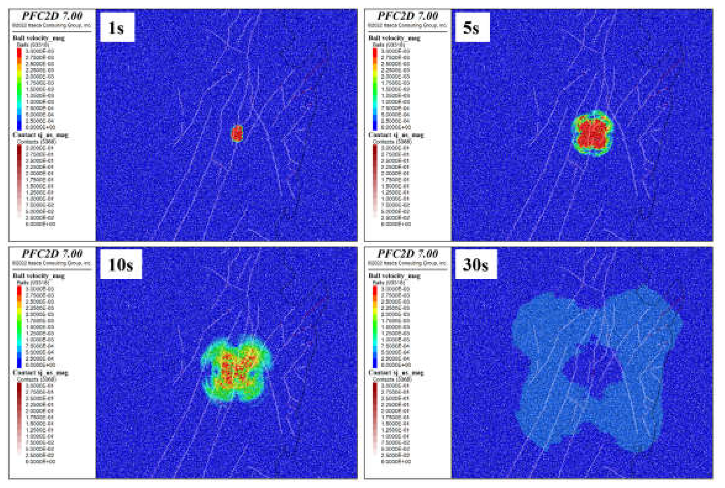
Figure 9.
Particle displacement vectors at 30 seconds after start of fault dynamic rupture.
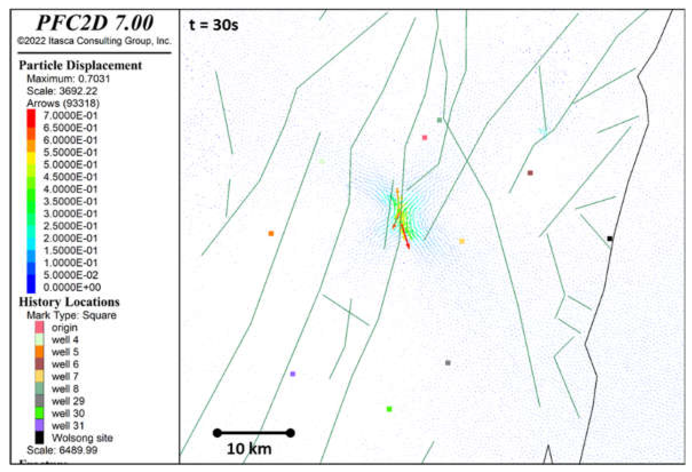
Figure 10.
Spatial distribution of pore pressure at simulation time of (a) 5, (b) 10, and (c) 15 seconds.
Figure 10.
Spatial distribution of pore pressure at simulation time of (a) 5, (b) 10, and (c) 15 seconds.
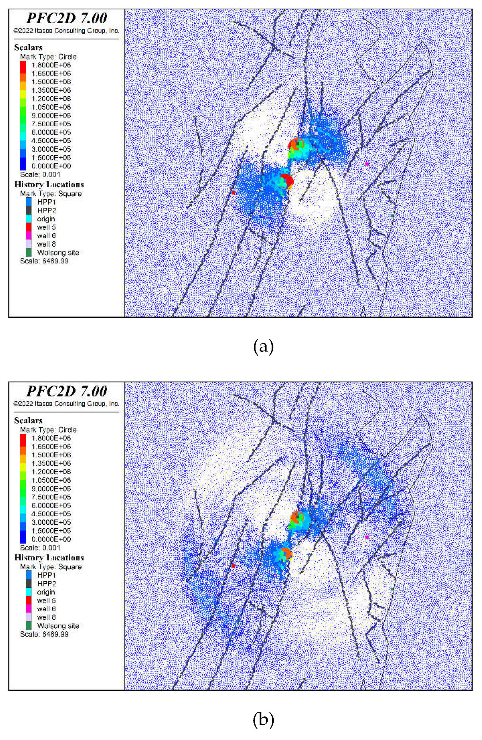
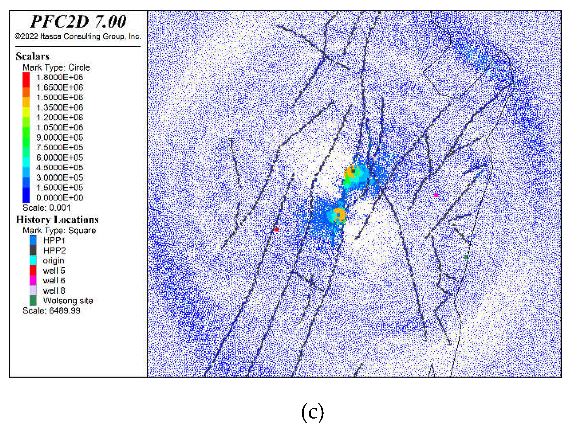
Figure 11.
(a) Pore pressure evolution simulated at the location of Well 8 in the model, corresponding to the location of Station 8 Gyeongju Cheonbuk, (b) groundwater level monitored at Station 8 Gyeongju Cheonbuk.
Figure 11.
(a) Pore pressure evolution simulated at the location of Well 8 in the model, corresponding to the location of Station 8 Gyeongju Cheonbuk, (b) groundwater level monitored at Station 8 Gyeongju Cheonbuk.
Disclaimer/Publisher’s Note: The statements, opinions and data contained in all publications are solely those of the individual author(s) and contributor(s) and not of MDPI and/or the editor(s). MDPI and/or the editor(s) disclaim responsibility for any injury to people or property resulting from any ideas, methods, instructions or products referred to in the content. |
© 2024 by the authors. Licensee MDPI, Basel, Switzerland. This article is an open access article distributed under the terms and conditions of the Creative Commons Attribution (CC BY) license (http://creativecommons.org/licenses/by/4.0/).
Copyright: This open access article is published under a Creative Commons CC BY 4.0 license, which permit the free download, distribution, and reuse, provided that the author and preprint are cited in any reuse.


