Submitted:
06 February 2025
Posted:
08 February 2025
You are already at the latest version
Abstract
Port pricing strategies are key tools for optimizing revenue, enhancing competitiveness, and ensuring efficient resource allocation. To help port operators effectively utilize the port yard, this paper investigates the port yard storage pricing problem under varying free storage periods and pricing strategy ranges. This problem involves a revenue game between the container yard (CY), remote container yard (RCTY), and carriers, in this game problem, each player has a large range of decision variables, which significantly increases the complexity of the entire problem. Based on carrier data from port services, we use a voting clustering approach to group multiple carriers, this can significantly reduce the pricing calculation complexity for port operators. Subsequently, we establish game-theoretic pricing models for CY, RCTY, and the carriers, both before and after the implementation of pricing clustering. During the pricing strategy simulation phase, we conduct sensitivity analysis on pricing ranges and free storage periods, using data from a port in Southeast China. The final conclusions related to port pricing are derived from this analysis, providing management insights for CY operators.
Keywords:
Port Pricing Strategies
; Voting Clustering
; Pricing Model
; Pricing Strategy Simulation
1. Introduction
In the ever-expanding global trade, ports serve as pivotal nodes in international commerce, assuming an increasingly vital role. Containerized cargo, being the predominant mode of goods transportation, significantly influences both port efficiency and operational costs. Data sourced from Clarkson illustrates the duration of stay for container vessels exceeding 8,000 TEUs worldwide, as depicted in Figure 1. Nevertheless, as cargo transportation continues to surge, the pricing issue for storage in port yards has become a prominent focus of attention. As Chen Xiyan [1] mentioned, zero demurrage fees will seriously affect the principle of equivalents for equivalents and is not conducive to the healthy development of the shipping market. This issue significantly affects all stakeholders, including transportation costs, logistics efficiency, port management, and various other factors, ultimately shaping port operations and international trade.
Containerized terminals are crucial components of port management, acting as hubs for goods and directly influencing transport efficiency. Port warehouses typically establish pricing standards for container storage, including two main factors: the duration of the free stack period and the charging standards after this period ends. Under these circumstances, port authorities set a specific period for free storage of containerized cargo at the terminal. Once this period ends, additional fees are charged to the carrier. For example, the port typically allows a seven-day grace period for container storage, after which a fee is incurred for delayed container removal. The fees correspondingly escalate with the duration of time elapsed. Yet, the increasing volume of container transport leads to varying approaches among port forwarders, resulting in a rising trend in the management and operational expenses associated with containerized cargo storage. This requires port administrative bodies and operators to reassess pricing policies, adopting a refined approach to operational management. Moving away from traditional uniform pricing, they seek a more effective payment model to support sustainable growth, balancing operational expenses and competitiveness, thereby improving service perception for shippers and carriers. There has also been research attention on the pricing methods for containerized yard operations. Lee, C.-Y. and M. Yu [2] studied the competition of storage prices for inbound containers between container terminals and remote container yards from the perspective of non-cooperative game theory. They assumed two scenarios for the pricing strategy of container storage, one independent of storage time and the other dependent on storage time. Subsequently, taking the competitive relationship between two shipping companies as motivation, they discussed the competition of storage prices for inbound containers, providing guidance for shipping companies in competitive situations regarding container storage. In addition, Cui, H. and T. Notteboom [3] studied the impact of different levels of service differentiation and port authority objectives (port ownership structure) under different port competition and cooperation environments. By comparing the benefits of competitive and cooperative sub-games, they provided a new perspective for promoting port cooperation by determining the feasible combination pricing of service differentiation and port ownership structure. However, these studies did not contemplate the disparate behaviors of the carriers; moreover, during the research process, a specific distribution was assumed for the container stay duration of the carriers’ containers at ports, without taking into account the actual port departure.
The objective of this paper is to conduct an in-depth examination of a specific case study at a southeastern port of China. By initially processing foundational data and employing principles from customer hierarchical theory and dynamic pricing theory, this study will investigate the differentiated pricing strategies of operators based on the integrated approach clustering. Specifically, the study aims to achieve the following three concrete objectives:
1. Concerning the duration of dwell time for a multitude of container types at this port, an investigation is conducted into the behavioral characteristics of the carriers, with the subsequent application of integrated clustering on such findings.
2.By integrating the clustering results, port warehouses will simulate dynamic pricing strategies for each carrier, aiming to capture their next-step decision-making behavior and trend.
3.Comparing the profitability before and after implementing differentiated services and dynamic pricing strategies in ports highlights the optimization effects achieved in terms of operating efficiency and operational outcomes.
Through the study of this piece, one may discern past inadequacies in addressing service-based differential pricing, thereby enriching the related theoretical concepts. Summarize the inadequacies of current research, delve deeper into the dynamic pricing strategies employed by ports, and enhance the study on the differentiation of port services. Moreover, to foster the advancement of practice through theory and to enhance its applicability, ensuring that theory can truly be executed and executed with precision for ports. Assist in recouping the expenses incurred due to service enhancement, and reap immediate profits. Provide an option for decision-making regarding the differential pricing of containerized goods at a certain port in the eastern corner of our nation.
2. Literature Review
We will classify literature related to research into two branches: (1) Differentiated service problem (2) Strategic port pricing.
2.1. Differentiated Service Problem
According to consumer theory, after segmenting customers, businesses mainly differentiate themselves from competitors through service and pricing. From a service perspective, different types of services are provided for different segmented markets, while from a pricing perspective, after segmenting customers, businesses use pricing strategies to achieve differentiation from other competitors. Shi Xin [4] proposed that when studying the differentiation of services between ports, attention should be paid to the mutual influence between different ports. Therefore, he constructed a two-stage game strategy model from the perspective of game theory to analyze the strategies and characteristics of port differentiation services. Yu, MZ, et al [5] studied the competition of regional container ports, and also involved that the two port cities each have their own container terminals. Finally, they gave management suggestions for the service tendency of each port. Wang Shenghua [6] considered the three competitive situations of differentiated competition, homogeneous competition and cooperation between the two duopoly ports, and came up with the differentiated competitive strategy when the service level of both port enterprises is the same. Propose differentiated strategies in the context of short-term market competition and long-term market competition. Wang et al [7] have developed key trade-offs for selecting pricing strategies in mixed hub ports, elucidating the application scenarios for differentiated pricing strategies. Ma Dongsheng et al [8] in response to the 'self-operated' and 'commission' models of platforms, have constructed two-period dynamic pricing game models respectively, to explore the interactive effects of BBP on external competition and internal cooperation of the platform. Yuan KB et al [9] studied four dynamic game scenarios of two adjacent ports. Using the dynamic game method, they compared the port service pricing, port demand and port profit under different competition and cooperation combinations, and finally obtained the behavior logic of the two ports in different situations.
In general, for the differentiation of ports, it mainly starts from the price and service, and considers the mutual competition and cooperation behavior between the two ports, but this paper is based on the differentiated pricing strategy of CY and RCTY, and introduces it into the system of CY, RCTY and carrier, in order to simulate how the pricing decision of CY affects the behavior of RCTY and carrier.
2.2. Strategic Port Pricing
For CY, on the one hand, it needs to provide container storage services to the carrier, on the other hand, it needs to make as much use of its own yard available space as possible, so it is necessary to influence the behavior of the carrier and RCTY through pricing strategies to achieve their own goals. For CY, however, choosing a pricing strategy is often a complex and time-consuming task that requires coordination with many stakeholders. Zhang, Q.et al [10], and Yang Shuwen [11] all conducted research on the storage pricing of import containers with different distributions of dwell time at the port, and proposed the pricing strategies of the liner company and the terminal in different situations through the Stackelberg game model. Gang Dong and Huang Rongbing [12] studied the optimization of inter-port pricing strategies in multi-port gateway areas (mpgr) and inter-container terminal pricing strategies in the context of deregulated port competitive service charges. The Nash equilibrium of the corresponding pricing strategy is obtained. Shaoqing Tian et al. analyzed supply chain pricing scenarios using a two-channel network model, contrasting blockchain and traditional distribution channels. Youn Ju Woo et al [13] studied the storage price scheduling problem for outbound container storage, by establishing a mathematical model to determine the optimal storage price list maximizes the total profit of the terminal or minimizes the total cost of the system. Wei Xing et al [14] analyzes the effects of integration between two neighbor ports with a third port sharing the same overlapping hinterland. Gang Dong et al [15] developed a game model under three different scenarios to analyze the tacit collusion between regional ports. Yang Hualong [11] investigated warehouse location pricing dynamics, demonstrating strategic customer retention thresholds in warehousing enterprises using Stackelberg game theory. Sun He and Zeng Qingcheng [16] explored pricing decisions under container storage competition considering both external and internal yard competitions through the construction of a container stacking pricing model. Yang Shuwen et al [17] and Zhang, Q et al [10] constructed a Stackelberg game model for the terminal yard and external yard under the consideration of storage demand changes, and studied customer storage behavior as well as pricing decisions for the terminal yard and external yard. In contrast, Giat,Y [18] classifies customers based on the amount of storage space they need, offering two different storage services for different types of customers. Kim, KH and Kim [19], Woo, YJ et al [13] have studied the method of determining the optimal price plan for imported containers in container yards. The profit or cost model of optimal price scheduling is established from the perspective of public terminal operators and private terminal operators respectively. Different from that, Martín, E et al [20] proposed a model to determine the optimal storage pricing schedule for imported containers. A general scheduling scheme is adopted, and the average speed and storage time charges are introduced into the random behavior of the yard for research. Yu, MZ, et al, studied a two-stage pricing game model involving a shipping company pursuing profit maximization and a container terminal operator. Wen, DP et al [21] developed a game-theoretic model to study the pricing problem in a supply chain considering environmental responsibility behavior, under both the fully rational and bounded rational scenarios. He,S and Ma,ZJ [22] discuss the relationship between the quality of service and pricing strategy of dual-head competitive CDPs in two different competitive scenarios. In addition, Jiang, LJ et al [23] considered the multi-type game relationship between the port group and multiple ports and customers in the time span planning, and proposed a three-layer planning model based on repeated game for the collaborative optimization of port procurement selection and service pricing in inland rivers. Nguyen, HO et al [24] divided the interaction between ports in the network into two stages, the analysis of price response function and the identification and interaction of network relations to analyze the price interaction between ports in the network.
In general, the existing research on the impact of changes in the pricing strategy of the port yard on the behavior of the distant outer yard and the carrier is less, even if there are a large number of studies on the differential pricing strategy of the port, but these studies are mostly based on the study of the carrier container stay time in the port, and rarely consider the actual data.
3. Problem Description
This paper provides a brief description of a unified pricing strategy for container storage at a port serving multiple carriers. The container dwell time for various carriers is denoted as , where =1,2,3,4,…. There is a remote container yard (RCTY) and an internal container yard (CY) at the port. The CY proposes its own pricing strategy, which primarily includes two decision variables: a uniform free storage period for all carriers, and a charging scheme for exceeding this free period. The specific fee structure is ), where is the fixed rate charged by the port's container yard to the carriers, and is the daily rate per container for each day it stays at the port beyond the free period.
During this period, carriers have the option to transport their containers to the remote yard (RCTY), with a unit transportation cost of per container. Simultaneously, the RCTY proposes its own container storage pricing strategy. Unlike CY, RCTY does not offer a free storage period, so its pricing strategy only includes the fee structure , where is the daily rate per container at RCTY starting from the moment when the container is transferred from the CY.
For carriers, the decision variable is the timing t at which the container should be transferred from the port's internal yard (CY) to the remote yard (RCTY). A detailed scenario description is illustrated in Figure 2.
3.1. Basic Assumptions
Based on the aforementioned problem description, several assumptions are made, as detailed below:
Assumption 1: The flow of all types of containers is stable and independent of storage prices. This assumption is widely applied in studies that utilize game theory to address the pricing of container storage fees at ports. For example, Chung-Yee Lee and Mingzhu Yu [2] indicated that the port's cargo flow is primarily influenced by the physical location of customers, the size of the local market, and the productivity of the container terminal. Therefore, assuming a stable flow of all types of containers independent of storage prices is reasonable.
Assumption 2: Unlike the internal container yard (CY), the remote container yard (RCTY), due to its special geographical location, is generally far from the port terminal. Consequently, it does not face limited and scarce storage space as CY does. Thus, we assume in this paper that the storage space of RCTY is unlimited. Based on this assumption, since RCTY's storage space is unlimited, the per-unit storage cost per unit time for containers at RCTY is also much lower than that at CY, i.e.,
Assumption 3: Unlike previous studies by Chung-Yee Lee and Mingzhu Yu 2and Youn Ju Woo [13], which consider homogeneous carrier behavior, this paper assumes heterogeneity in carrier behavior. Specifically, the distribution of container dwell times at the port varies among different customers. This heterogeneity is a significant highlight and starting point of this paper, making the study more closely aligned with actual data.
Assumption 4: Utilizing container dwell time data from a port in the southeastern coastal region of China, we plotted a histogram showing the distribution of container dwell times at the port. Based on the shape of the histogram, we used k-means clustering to classify carriers into different types, each with its own pricing strategy.
Assumption 5: For each type of carrier, the container dwell time at the port is a random variable. Each carrier transports containers from the port’s internal yard to the external yard in batches, without needing to decide on the quantity of containers to be transferred.
3.2. Data and Clustering
To verify that Assumption 4 aligns with the actual port operations, we selected dwell time data for four types of containers from a port in the southeastern coastal region of China. Based on the actual situation, this port only charges storage fees for imported containers staying in the port, so the focus of our study in this article is on imported containers, not exported containers. The specific data are illustrated in Figure 3 and Figure 4.
3.2.1. Data Presentation
The data sets used in this study represent the dwell times of different container types at the port. Each figure (Figure 3 to Figure 4) illustrates the distribution of container dwell times for one of the two types of containers. These distributions provide insights into the operational patterns and characteristics of each container type at the port.
By visually examining the histograms of the dwell times for the two types of containers handled by different carriers, we observe significant differences in the dwell times both among different carriers and across different container types. These observations provide a practical basis for our clustering approach. Through clustering, we can classify different carriers handling the same type of container, thereby facilitating differentiated pricing strategies.
3.2.2. Clustering Criteria and Results
Next, we introduce the voting-based clustering method employed in this paper. Initially, multiple clustering algorithms (K-means, BIRCH Clustering, and Gaussian Mixture Model) are used to cluster the data. Each sample's clustering results are then subjected to a voting process, and the category with the most votes is assigned as the final clustering label for that sample. The choice of these three clustering models is strategic, as each has distinct advantages and limitations. By using a voting method, we can leverage the strengths of each algorithm to enhance the accuracy and robustness of the clustering results.
K-means Algorithm: K-means is highly scalable and its results are easy to interpret. However, it performs poorly with non-spherical clusters and is sensitive to outliers and noise.
Gaussian Mixture Model (GMM): GMM can identify non-spherical clusters and does not assume any particular shape for clusters, making it flexible and less affected by outliers and noise. Its drawbacks include the need to pre-specify the number of mixture components and potential issues with local optima.
BIRCH Clustering: BIRCH is robust to noisy data and does not require pre-specifying the number of clusters. It is more suited for convex-shaped clusters and might not perform well with non-convex clusters.
The combination of these three algorithms compensates for their individual weaknesses, making the clustering results more reliable.
The final clustering result is determined by using the clustering outcome with the minimum Davies-Bouldin Index as the baseline. The results from the other two clustering methods are then used to adjust the final clustering. The Davies-Bouldin Index (DBI) is a clustering evaluation metric that measures the performance of a clustering algorithm by considering the ratio of within-cluster tightness to the separation between clusters. Specifically, for each cluster, DBI calculates the average distance of all points in the cluster to the cluster center (tightness) and compares it with the average distance to the centers of other clusters (separation). For each cluster, DBI considers the separation from the nearest cluster. The overall DBI is the average of these ratios for all clusters, with lower values indicating better clustering performance.
To ensure the stability of the clustering results, random parameters were set for each algorithm, guaranteeing that the results remain optimal and consistent across runs. Additionally, grid search was employed to fine-tune the parameters for each clustering algorithm, using the Davies-Bouldin Index as the evaluation criterion. This comprehensive approach ensures that the clustering results are robust, reliable, and reflective of the actual data patterns.
Davies-Bouldin Index:
A metric to evaluate clustering quality by comparing within-cluster tightness and between-cluster separation. Lower DBI values indicate better clustering performance.
A metric to evaluate clustering quality by comparing within-cluster tightness and between-cluster separation.
Calculated by:
where and are the average distance of all points in clusters and to their respective centroids, and is the distance between the centroids of clusters and .
In the clustering process, we focus on the dwell times associated with different SERVICE_CODES. The features selected for clustering include the container volume for each SERVICE_CODE, as well as the statistical distribution information of dwell times and container counts. These features primarily comprise the mean, standard deviation, kurtosis, and skewness of the dwell times and container count, refer to Table 1 for details.
Clustering Features:
Container Volume (for each SERVICE_CODE): The total number of containers associated with each SERVICE_CODE.
Dwell Time Distribution Statistics:
Mean Dwell Time: The average time containers associated with a specific SERVICE_CODE spend at the port.
Standard Deviation of Dwell Time: Measures the variability or dispersion of the dwell times.
Kurtosis of Dwell Time: Indicates the "tailedness" of the distribution of dwell times.
Skewness of Dwell Time: Measures the asymmetry of the distribution of dwell times.
Container Count Distribution Statistics:
Mean Container Count: The average number of containers that have specific dwell times.
Standard Deviation of Container Count: Measures the variability in the number of containers for different dwell times.
Kurtosis of Container Count: Indicates the "tailedness" of the distribution of container counts across different dwell times.
Skewness of Container Count: Measures the asymmetry of the distribution of container counts across different dwell times.
Clustering Algorithms:
K-means: Suitable for identifying spherical clusters; sensitive to outliers and noise.
BIRCH (Balanced Iterative Reducing and Clustering using Hierarchies): Effective for large datasets and robust to noise; suitable for convex-shaped clusters.
Gaussian Mixture Model (GMM): Capable of identifying non-spherical clusters and flexible in cluster shape assumptions; less affected by outliers and noise.
Voting-Based Clustering:
Apply all three clustering algorithms to the datasets. For each sample, assign the final cluster label based on the majority vote from the three algorithms.
Evaluation and Adjustment:
Use the clustering result with the minimum Davies-Bouldin Index (DBI) as the baseline. Adjust the final clustering labels by considering the results from the other two clustering methods.
Parameter Tuning:
Conduct grid search to optimize parameters for each clustering algorithm using DBI as the evaluation metric. Set random parameters to ensure consistent and optimal clustering results. By integrating these features and methodologies, the clustering process ensures a robust, accurate, and meaningful classification of the dwell time patterns for different SERVICE_CODEs, enabling effective differentiated pricing strategies.
Thus, the introduction to the integrated clustering is roughly complete. Next, we will present the optimal parameters for the three clustering algorithms, the clustering results corresponding to these optimal parameters, the Davies-Bouldin values, and the adjusted Davies-Bouldin value after integration.
The introduction of the clustering methods and evaluation metrics used in the article is now complete. Next, the optimal parameters, clustering results corresponding to the optimal parameters, and the Davies-Bouldin values for four clustering algorithms will be presented.
From the perspective of the four clustering algorithms of Import shipping container, K-means uses the k-means++ initialization method to ensure that the selection of the initial cluster centers is more optimal, and finds the optimal clustering by setting 3 clusters and multiple initializations, with a moderate clustering effect. The Birch algorithm performs hierarchical clustering in the tree structure, with a branching factor of 50 and a threshold of 0.1, and the clustering effect is poor. The Gaussian Mixture model assumes that the data comes from multiple Gaussian distributions, and 'tied' covariance type means that all Gaussian distributions share the same covariance matrix. Using k-means to initialize the parameters for pre-processing, the clustering effect is slightly better than K-means. Voting clustering combines three clustering algorithms to improve the clustering effect, which is the best among the four algorithms.
Meanwhile, the four clustering algorithms used in import empty container were evaluated. K-means utilized the random initialization method and set 9 clusters with 15 initializations to find the optimal clustering, resulting in moderate clustering outcomes. The Birch algorithm performed hierarchical clustering in a tree structure, but yielded poor clustering results. The Gaussian Mixture model assumed that the data originated from multiple Gaussian distributions, and used 'spherical' covariance_type to indicate that each Gaussian distribution had its own independent variance. By using k-means initialization parameters for pre-processing, the clustering effect was slightly better than that of K-means. Integrated Clustering combined multiple clustering algorithms to improve the clustering effect, with the service code set to 10 classes, resulting in the best clustering effect.
According to the data and our assumptions, the whole problem can be structured as follows: before clustering, CY and RCTY propose corresponding pricing strategies for each carrier, and then the carriers adjust their own transfer time based on the pricing strategies. CY and RCTY then readjust their pricing strategies based on the carriers' adjusted transfer time, and this cycle continues until a stable state is finally reached. The only difference in clustering is that the original research object is changed from a single carrier to a group of carriers within a cluster, and the data of the carriers within a cluster is treated as a whole, with CY and RCTY proposing corresponding pricing strategies, and the determination of the cyclic state and stable state is consistent with the pre-clustering. Throughout the process, CY maximizes its own revenue, RCTY maximizes its own income, and the carriers minimize their own costs.
4. Modeling
In the previous chapters, we have conducted a cluster analysis on the container dwell time of different carriers in a port. This chapter will model the problem studied in this paper, and the specific problem scenario is the same as described in Chapter 3. Below are some of the parameters and decision variables of the model.
4.1. Game Model Before Clustering the Carriers
Model Parameters:
: The number of port service carriers
The number of categories formed after clustering the carriers, where = 1, 2, …… C
: The available space in port that CY has designated for storage purposes.
: The available space in port that RCTY has designated for storage purposes. This is set to an infinite value
: The maximum value of the variable cost of per container storage in the CY
: The minimum value of the variable cost of per container storage in the CY
: The maximum value of the fixed cost of per container storage in the CY
: The minimum value of the fixed cost of per container storage in the CY
: The maximum value of the variable cost of per container storage in the RCTY
: The minimum value of the variable cost of per container storage in the RCTY
: The maximum value of the fixed cost of per container storage in the RCTY
: The minimum value of the fixed cost of per container storage in the RCTY
: The container free storage period in the port yard (CY) is set for all carriers before the carrier clustering.
: The free storage period for containers set for the-th class of carriers after clustering the carriers in the port yard
: The maximum dwell time for all carriers at the port before the clustering
: The maximum dwell time for Category carrier at the port after the clustering
: Probability density function of import shipping container dwelling time at port before the clustering for carrier j.
: Probability density function of import empty container dwelling time at port before the clustering for carrier j.
: Probability density function of the import shipping container dwell time at the port for category carrier after the clustering.
: Probability density function of the import empty container dwell time at the port for category carrier after the clustering
: The unit container transportation cost of carrier transferring the container from the port yard CY to the remote yard RCTY before the clustering.
: The unit container transportation cost of carrier of category transferring the containers from the port yard CY to the remote yard RCTY after the clustering.
Decision Variables:
: CY in the port yard charges variable cost per container per day set in the storage fee for carriers before the clustering.
:CY in the port yard charges a fixed cost set in the storage fee for carriers before the clustering.
: RCTY in the port yard charges variable cost per container per day set in the storage fee for carriers before the clustering.
: RCTY in the port yard charges a fixed cost set in the storage fee for carriers before the clustering.
:CY in the port yard charges variable cost per container per day set in the storage fee for category carrier after the clustering.
: CY in the port yard charges a fixed cost set in the storage fee for category carrier after the clustering.
: RCTY in the port yard charges variable cost per container per day set in the storage fee for category carrier after the clustering.
: RCTY in the port yard charges a fixed cost set in the storage fee for category carrier after the clustering.
: The optimal transfer time determined by carrier based on the pricing strategy of CY and RCTY before the clustering.
: The optimal transfer time determined by the pricing strategy of CY and RCTY made by category carrier after the clustering.
Objective Function:
:CY in the port yard charges fee for carrier before the clustering, or the revenue CY receives from carrier .
: RCTY in the port yard charges fee for carrierbefore the clustering, or the revenue RCTY receives from carrier : The detention fee for containers at the port before the clustering.
:CY in the port yard charges fee for category carrier after the clustering, or the revenue CY receives from category carrier.
: RCTY in the port yard charges fee for category carrier after the clustering, or the revenue RCTY receives from category carrier.
: The detention fee for category carrier at the port after the clustering.
Specifically, there are three main time points: the free storage period set by the CY, the container's stay time in the port, and the time when the carrier transfers the container from the CY to the RCTY. The revenue function of the CY inside the port obtained from the carrier before the clustering is as follows.
Meanwhile, also mainly involves three time points: the container's stay time in the port, the time for the carrier to transfer the container from the CY to the RCTY and the maximum value of the container's dwell time. The revenue function obtained by the port from carrier before the clustering at the RCTY is as follows.
For the carrier, the key three time points involved are the container's stay time ,the carrier's own transportation time and the free storage period set by the CY. The cost function carrier to pay before the clustering is as follows
For RCTY, the variable and fixed costs of unit container storage should be limited within a certain range, so there are
In addition, considering the actual scenarios, CY's price setting on storage fees will be significantly higher than RCTY, so there are
Considering the transfer time of the carrier, there should be
Therefore, for the RCTY, its optimization model is as follows
The constraints of the model are defined by (2)-(6).
For carriers, the constraints on pricing of CY and RCTY should also be met, so the constraints of the model are defined by (2)-(6). In addition, the carrier also needs to make decisions about its own transfer time, there should be
Constraints (7)-(9) characterize the transfer strategy of the carrier, who will only choose to transfer if the revenue of the port's yard plus the transfer cost is greater than or equal to the revenue of the yard outside the port.
Therefore, for the carrier, its optimization model is as follows
The constraints of the model are defined by (2)-(9).
4.2. Game Model with Clustering of Carriers
In the previous section, we have already explained the basic parameters of before the clustering. Therefore, this section will only briefly discuss the changes in the objective function and constraints after clustering.
The revenue function of the CY inside the port obtained from the carriers after the clustering is as follows.
For RCTY, constraints (2) before the clustering are replaced by constraints (10), constraints (3) are replaced by constraints (11), they represent the same meaning, only the objects being constrained have changed.
In addition, constraint (4) before the clustering is replaced by constraint (12), constraint (5) is replaced by constraint (13) and constraint (6) is replaced by constraint (14).
So, for the RCTY, its optimization model after the clustering is as follows:
The constraints of the model are defined by (10)-(14).
For carriers, before the clustering, constraint (7) is replaced by constraint (16), and constraint (8) is replaced by constraint (17).
So, for the carriers, its optimization model after the clustering is as follows:
The constraints of the model are defined by (9)-(17).
With this, we have clarified the parameters, decision variables, and model descriptions involved in this article. By simulating the parameters of the CY and optimizing the game with the RCTY and the carrier, we seek a series of Nash equilibrium points: the optimal dwell time of the carrier under the given charging strategy of the CY and the RCTY. At this Nash equilibrium point, both the port internal yard and the distant external yard aim to maximize their total charging fees, while the carrier aims to minimize its total payment.
4.3. Analysis of Participant Strategy Sets
In this part, we will start from the strategy set of the three parties, and analyze the importance of clustering the carriers from the perspective of computational complexity.
For the CY, the main strategies it can choose include setting the free storage period for containers and obtaining revenue by adjusting its own pricing strategy. Based on the comparison of storage fees at major seaports in 2019, we know that the free storage period for imported containers in Yantian Port is generally 8-11 days, and the storage fee per container unit changes in a stepped manner after the free storage period, with a fee of 125 yuan per day from 8 or 11 to the 15th day, and 245 yuan per day after the 15th day. Therefore, when formulating the pricing strategy for the container yard, the strategy set for the free storage period for containers is {5,6,7,8, 9, 10, 11,12} days, and the pricing strategy (, ) is set, where the fixed cost should not be greater than this value. We set the fixed cost from 8 or 11 days to the 15th day as [100, 125], and the variable cost as [0, 25]. We set the fixed cost after the 15th day as [200, 245], and the variable cost as [0, 45]. Therefore, we have the following stepped function for the unit container fee in the CY.
For RCTY, in practice, since it does not set a free storage period and the available storage space is much larger compared to CY, the pricing strategy generally does not exhibit a step-like change trend, but rather is 1/2 or 1/5 of the CY pricing strategy. Therefore, we set the range of to (0, 10) and the range of to (0, 50). There is also a possibility of small fluctuations, which we will adjust in subsequent numerical experiments. This ensures to a certain extent that the strategy sets of the three parties in the game are limited. Therefore, we have the following stepped function for the unit container fee in the RCTY.
Next, we will discuss the differences in terms of computational complexity between before and after clustering carriers when setting up the pricing strategy. If we formulate a pricing strategy for all carriers without conducting layered pricing, it means that each carrier will have two decision variables: and (to CY), and (to RCTY). Therefore, if there are N carriers, all N carriers will have 2N decision variables. Assuming each decision variable and has m possible values, the total number of decision combinations will be , which means that adding one more carrier will increase two more decision variables, and each variable has m possible values, which is clearly an exponential growth. After clustering pricing, by clustering carriers, the value of is reduced to the clusters , where << , which greatly reduces the computational complexity of the problem.
Specifically, by reducing and mapping the pricing problem studied in this paper to other NP-hard problems, it can be simply mapped to the set cover problem. In the set cover problem, we have a universal set {} and a series of subsets , and the goal is to find the smallest subset collection such that the union of these subsets equals the universal set {}.In our problem, the time each carrier's container spends in the port can be seen as elements in the universal set {}, while each carrier's cost decision {(,)} can be seen as a subset {}. Our goal is to find a set of cost decisions that maximizes the utility of all carriers while maximizing the port's revenue from the carriers.
An instance of the set cover problem can be represented as {()}, where {} is the universal set, {} is the collection of subsets, and {} is the size of the required collection of subsets.
The definition of the complete set {}: The complete set {} consists of the total dwell time of all carriers' containers in the port
The definition of a subset : Each subset corresponds to the pricing decision for each carrier.
The definition of the size limit of the subset collection: The subset that maximizes the revenue of CY within the port and the subset that maximizes the revenue of the RCTY in the pricing decision.
Therefore, we can say that the pricing decision of the carrier studied in this paper can be reduced to the set covering problem, and the set covering problem is a typical NP-hard problem. Thus, as continues to increase, the pricing decision of the carrier, like the set covering problem, cannot be solved in polynomial time, which further illustrates the necessity of clustering the carriers.
After clustering the carriers, the value of is reduced to the clusters , which will greatly reduce the computational complexity of the problem. The main research object has shifted from the original individual carriers to each cluster after clustering, and the constraints have basically remained unchanged.
5. Numerical Experiments
This section introduces the computational experiments conducted to evaluate the proposed game pricing. The experiments are divided into two main scenarios: the mathematical models before and after the after clustering is applied. The program was run on a computer equipped with a 12th Gen Intel(R) Core(TM) i5-12400F processor at 2.50 GHz and 16 GB RAM, running the Windows 11 operating system, version 23H2. The system is a 64-bit operating system based on an x64 processor. All carrier containers staying in the port data comes from real data of a port along the southeast coast of China.
5.1. Data Description
In Figure 6 and Figure 7, we have described the data of the imported containers, in section 4.3, we also described the range of values for container free storage period, , and .In order to further simulate the pricing of the container yard in the port, we will gradually adjust the range of free stacking period, and .The specific results will be presented in the following section.
5.2. Simulation of Parameters in the CY
Next, we will focus on the perspective of CY and conduct simulation based on the parameters of container free storage period and CY pricing strategy for before the clustering model. RCTY and carriers will optimize using genetic algorithms, adaptive genetic algorithms, etc. In this case, the crossover rate for genetic algorithms is set to 0.8, and the mutation rate is set to 0.2. The adaptive genetic algorithm will adjust the crossover rate and mutation rate based on the iterative process. In the initial stage of the algorithm, a higher crossover rate and mutation rate are used to explore the search space and introduce diversity to prevent the population from falling into local optimal solutions. In the later stages of the algorithm, a lower crossover rate and mutation rate are used to refine the search, ensuring convergence to the global optimal solution and avoiding excessive random disturbances.
5.2.1. Before the Clustering
This section presents the impact of pricing strategy scope and free stacking period on the objective functions of port yard revenue before hierarchical pricing, revenue from distant external yards, and carrier costs. It is expected to draw some conclusions on the pricing strategy setting for port yards in terms of port operation pricing strategy. There are nine main scenarios in which the sensitivity of pricing strategies changes.
Apart from the different value ranges, the logic of the values is the same as previously described.
First, we start with the import empty containers before clustering and observe the changes in the income of the CY, the income of the RCTY , the carrier’s storage costs, and the transfer time of each carrier as the carrier pricing strategy range varies before clustering. The following images display the data for each cluster, showing the carriers included in each cluster, as shown in Figure 7.
From Figure 7, we can see that before clustering the carriers, the changes in CY’s income under different pricing strategy ranges vary for different carriers. For most carriers, adjusting the pricing strategy range shows that changes in the pricing strategy range have a greater impact on CY’s income than changes in the pricing strategy range, especially for carriers like OUSE2 and TEC4. This indicates that before clustering, CY should consider the impact of variable costs in storage fees on its own income when setting pricing for similar carriers.
However, there are also cases where changes in the a1 pricing strategy range have less impact on CY’s income than changes in the b1 pricing strategy range, such as with the carrier MORC2. This suggests that such carriers are more affected by changes in fixed costs. Therefore, when adjusting the pricing strategy range before clustering, CY can consider increasing fixed storage costs to boost its storage income to some extent.
Additionally, there are cases where CY’s income from carriers is not affected by the pricing strategy range, such as with carrier CVX1. This may be because all containers of this carrier fall within the free storage period set by CY. If CY wants to increase its income, it could consider shortening the free storage period.
From this, we can draw
Result 1: If CY wants to increase its storage income before clustering, it should optimize the pricing strategy range based on the characteristics of different carriers' pricing strategies to maximize income. It can also be observed that without pre-clustering the carriers, this process may be relatively complex.
Let's first look at the changes in the RCTY’s income under different pricing strategies for import empty containers before clustering, as shown in Figure 8.
From Figure 8, we can see that due to the free storage period setting, most carriers choose to transfer containers from CY to RCTY, allowing RCTY to also gain storage income. For carriers like EUXT, when CY adjusts the pricing range for, the impact on RCTY's income is actually smaller than the impact of adjusting the b1 range. However, for most carriers, adjusting the a1 range in CY has a greater impact on RCTY's income than adjusting the range. There are also cases where no matter how CY adjusts the pricing strategy range, RCTY's income remains unaffected. This can be due to two reasons: one is that the carrier's container stays in port for a shorter time than CY's free storage period; the other is that the carrier's storage cost at CY is less than or equal to its transfer cost plus storage cost at RCTY. In summary, this means that the costs incurred by carriers for storing containers at CY are within their acceptable range. Based on this analysis, we can draw result 2 for CY.
Result 2: The impact of adjusting the pricing strategy range on RCTY's income should be considered in relation to specific carriers. This situation, which takes into account RCTY's income, is more complex and can be seen as an extension of result 1.
Specifically, for carriers like EUXT, CY operators can increase their income by adjusting the range of the pricing strategy without significantly affecting RCTY's income. This facilitates reaching more acceptable agreements with RCTY. On the other hand, when forming an alliance with RCTY, CY operators can use this strategy adjustment to strengthen their cooperation with RCTY, achieving a win-win situation for both parties. In forming an alliance with RCTY, focusing on adjusting thepricing strategy allows CY operators not only to increase their own income but also to minimize the negative impact on RCTY's income. This approach helps CY operators to establish a more stable and cooperative alliance with RCTY, creating more favorable conditions for long-term development. For carriers like MORC2, CY operators can adjust thepricing strategy range to increase its income, but attention should be paid to the critical point to avoid charging too high a fee, which could lead to early transfers by the carrier.
Next, let's first look at the changes in the carrier's costs under CY’s different pricing strategies for import empty containers before clustering, as shown in Figure 9.
From the figure 9, We can observe that the carrier costs are significantly affected by the pricing strategy range set by the CY. This indicates that most carriers are highly sensitive to the variable costs of container dwell time at the port. This is likely because the variable cost is the per-unit-time storage cost for a container at the CY, which increases substantially with the number of containers and the length of time the containers stay at the CY. As a result, this variable cost plays a large proportion in the carrier's overall cost calculation. It can be concluded the result 3
Result 3: For most carriers, the impact of the pricing strategy range change ofon carrier costs is smaller than the impact of the pricing strategy range change offor imported empty containers.
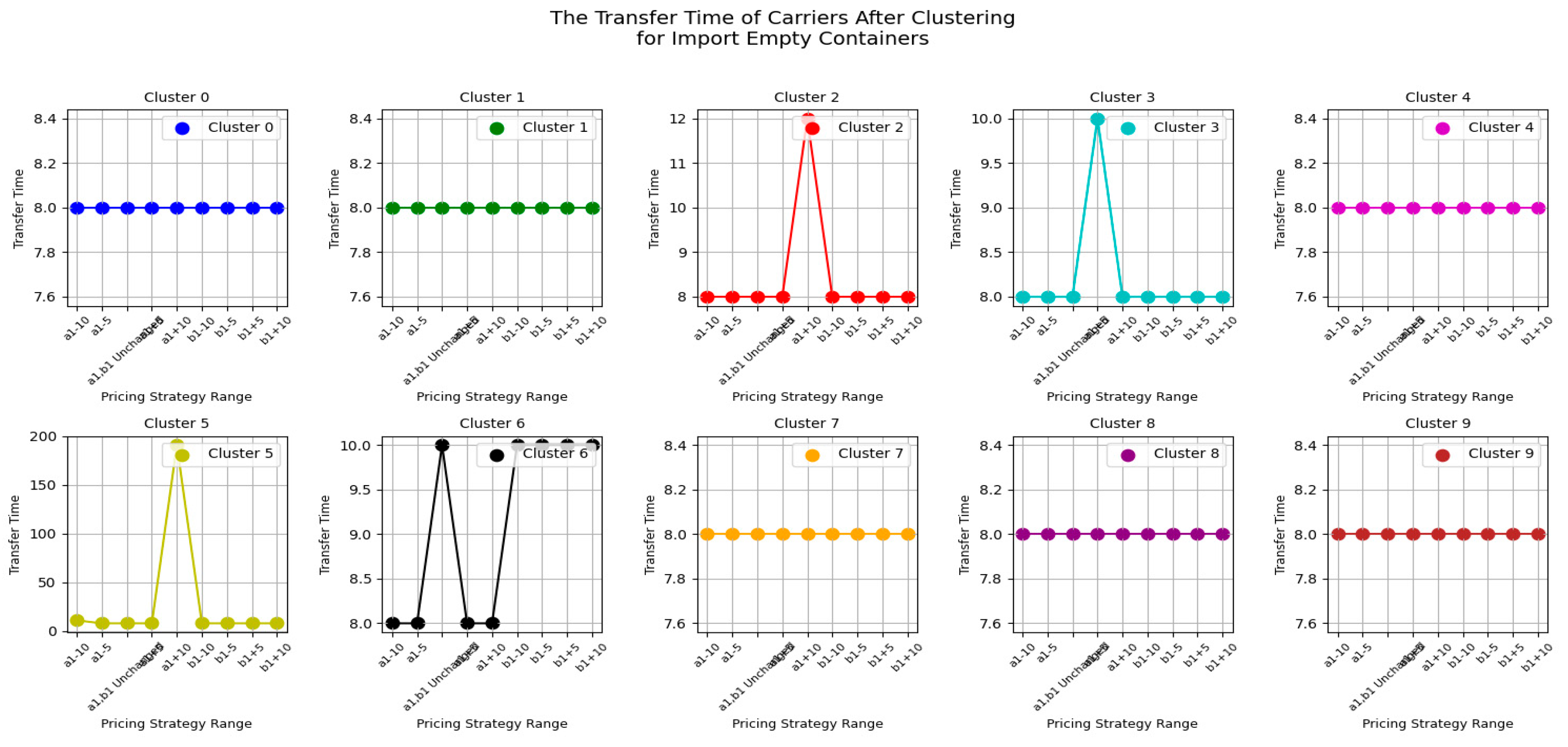
Next, let's first look at the changes of the carrier's transfer time under CY’s different pricing strategies for import empty containers before clustering, as shown in Figure 10.
From Figure 10, we can see that the transfer time of most carriers is not affected by the CY pricing strategy range. However, there are also carriers whose transfer time is significantly influenced by the pricing strategy range. It can be concluded the result 4
Result 4: For most carriers, the pricing strategy range variation for importing empty containers does not affect the transfer time of carriers.
Therefore, CY operators should prioritize adjusting the a1 pricing strategy to increase their own revenue while reducing carrier costs. This adjustment not only helps enhance CY's profitability but also reduces the financial burden on carriers, thereby improving the cooperation with them. Simultaneously, pay attention to the impact of a1 pricing strategy on a portion of carrier transfer time, to consider the sensitivity of different carriers to pricing strategy changes, and to avoid excessive adjustments to the a1 pricing strategy that could lead to instability in carrier transfer times, thus impacting overall operational efficiency. When adjusting the a1 pricing strategy, CY operators need to balance reducing carrier costs with maintaining stable transfer time. Proper adjustment of the a1 strategy can increase income while ensuring stable transfer time for carriers, which helps in fostering long-term cooperation with them.
Next, let's take a look at the impact of changes in the free storage period on a range of participants for empty container. Firstly, take a look at the impact of the free storage period change on CY's income .
From Figure 11, we can observe that for most carriers, the CY Income gradually decreases as the free storage period increases, such as in the case of AM2E. However, there are also carriers whose CY Income peaks at a certain free storage period and then declines, such as OUSE2. In addition, some carriers, such as CVX1, show no change in CY Income regardless of the free storage period.
Result 5: Overall, the CY Income exhibits different trends of change with the free storage period due to the specific characteristics of different carriers, necessitating a detailed analysis.
Let's take a look at the impact of the free storage period change on RCTY's income for import empty containers, as shown in Figure 12.
From Figure 12, we can see that most RCTY's income decreases with the increase in the free storage period set by CY. This is because, as CY extends the free storage period, more carriers opt to store containers in port storage yards, leading to a simultaneous decline in both CY’s income and RCTY’s income.
Result 6: For import empty containers, the RCTY’s income decrease with the increase of the free storage period set by CY.
Insights CY Operators when adjusting the free storage period, CY operators need to consider the acceptable range of income fluctuations and plan accordingly to avoid significant reductions in income due to these adjustments. In addition, if CY operators seek to form an alliance with RCTY and adjust the free storage period as part of the pricing strategy, they should consider compensating RCTY for any potential losses resulting from longer free storage periods. However, if the free storage period is relatively short, CY’s yards might still have sufficient space for other port operations, making it easier to manage available space effectively.
Next, let's take a look at the impact of free storage period on carrier’s costs and on carrier’s transfer time for import empty containers from Figure 13 and Figure 14.
Figure 13 and Figure 14 are more intuitive compared to the previous ones, directly supporting Result 7:
Result 7: The costs for most carriers decrease as the free storage period set by CY increases, while their transfer times increase.
This aligns with intuition: when CY extends its free storage period, carriers are more inclined to store containers in port storage yards. This not only facilitates their operations but also reduces container storage costs. However, due to CY's storage space limitations, there may be situations where containers must be transferred, resulting in increased carrier costs despite the extended free storage period.
Insights for CY Operators ,extending the free storage period can reduce the carrier's costs, which is beneficial for improving the carrier's service experience, help carriers reduce costs, thereby enhancing their competitiveness and willingness to cooperate. However, extend the free storage period could lead to a decline in port operation efficiency, as longer storage time may occupy more yard space, affecting the overall port operations. CY operators need to find a balance between extending the free storage period and maintaining efficient port operations, ensuring that carrier service experience is improved without compromising overall port efficiency. Through refined management and strategic adjustments, CY operators can meet the needs of carriers while maintaining their own operational stability.
Next, let's take a look at the import shipping container.
Figure 15Figure 16Figure 17 and Figure 18 show the impact of changes in pricing strategy range on the income of CY, the income of RCTY, the costs of carriers, and the transfer time of carriers for import shipping containers.
From Figure 15 and Figure 16, we can observe that for import shipping containers, the impact of CY adjusting the pricing strategy range of on its income and RCTY’s income are significantly greater than the impact of adjusting the pricing strategy range of . Generally, the income CY obtains from most carriers increases as the range of increases and decreases as the range of decreases. In contrast, the trend of CY's income variation with changes in the pricing strategy range of is less pronounced.
From Figure 17 and Figure 18, we can observe that carrier’s cost decrease as the range of / pricing strategy decreases, and increase as the range of pricing strategy increases for most carriers. In comparison, CY's adjustment of pricing strategy ranges has a relatively smaller impact on carriers' transfer time. Thus, result 8 is derived.
Result 8:The impact of the pricing strategy range change ofon the income of CY and income of RCTY for the import shipping container is smaller than the impact of the pricing strategy range change ofon them. In addition, changes in the pricing strategy range of CY have no impact on the transfer time of carriers.
Insights for CY operators to focus on the critical impact of the pricing strategy, when adjusting pricing strategies, CY operators should prioritize adjusting because it has a more significant impact on the overall system. Particularly, changes in of range can notably affect CY's income and carrier costs, and a well-adjusted a1 strategy can lead to more effective revenue management. In addition, CY operators need to carefully balance these two aspects when adjusting the b1 strategy to ensure that while increasing revenue, carrier costs are not excessively increased, which could negatively affect relationships with carriers. If CY operators wish to influence RCTY's income through pricing strategies, adjusting the a1 pricing strategy may be a more effective approach.
Next, let's look at the impact of sensitivity changes during the free storage period on the income of CY, the income of RCTY, the cost of the carrier, and the transfer time of the carrier for the import shipping container.
From Figure 19 to Figure 21, we can generally see that for almost all carriers, CY's income, RCTY's income, and the carrier's costs decrease as the free storage period set by CY increases. This is relatively simpler compared to the complex situation with import empty containers. However, in terms of RCTY's income, there are special cases for carriers like YHWP and THE4, which require separate discussion. There are two scenarios regarding the change in transfer time. In one scenario, the carrier's transfer time increases as the free storage period set by CY increases. In the other scenario, the carrier's transfer time remains unchanged regardless of the free storage period set by CY. The latter case may occur when the containers' dwell time at the port is relatively short, such that the dwell time for all containers of the carrier falls within the free storage period. Therefore, we can get result 10.
Result 10: CY's income, RCTY's income and carrier’s cost decrease as the free storage period increases.
This result provides the insights for CY operators that extending the free storage period may bring in less income, it can reduce carriers' costs to some extent, it may result in the port yard not being effectively utilized, potentially significantly reducing CY's operational efficiency. CY operators need to find a balance between the length of the free storage period, the availability of yard space, the carrier's costs and CY’s income.CY operators can consider closely collaborating with RCTY to jointly develop and adjust the free storage period strategy. This cooperation can not only help optimize overall income but also effectively manage yard space, avoiding issues of insufficient yard space caused by extended transfer time.
In general, in this section we explored the impact of the sensitivity of two different container types pricing strategy scope and free storage period sensitivity before the clustering to the income of CY, the income of RCTY, the carrier's cost, and the carrier's transfer time, providing CY’ managers with some insights into pricing strategies through relevant conclusions.
In the next section, we will explore the series of impacts and corresponding conclusions after the clustering to see if there are any differences between the two.
5.2.2. After the Clustering
Changes in sensitivity to price range and sensitivity to free storage period after the clustering has been shown in Table 3 and Table 4.
Next, let's look at the impact of sensitivity changes during the pricing strategy scope on the income of CY, the income of RCTY, the cost of the carrier, and the transfer time of the carrier for the import empty container after the clustering.
Figure 23.
The CY’s income under different pricing strategy scope for import empty containers after the clustering.
Figure 23.
The CY’s income under different pricing strategy scope for import empty containers after the clustering.
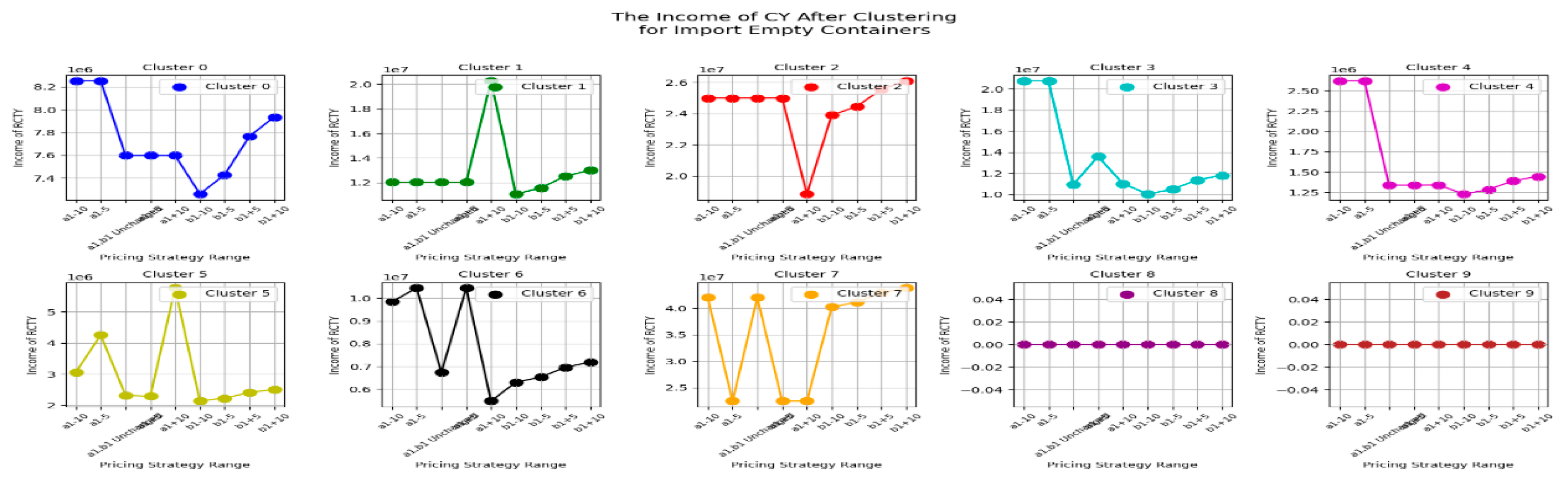
Figure 24.
The RCTY’s income under different pricing strategy scope for import empty containers after the clustering.
Figure 24.
The RCTY’s income under different pricing strategy scope for import empty containers after the clustering.
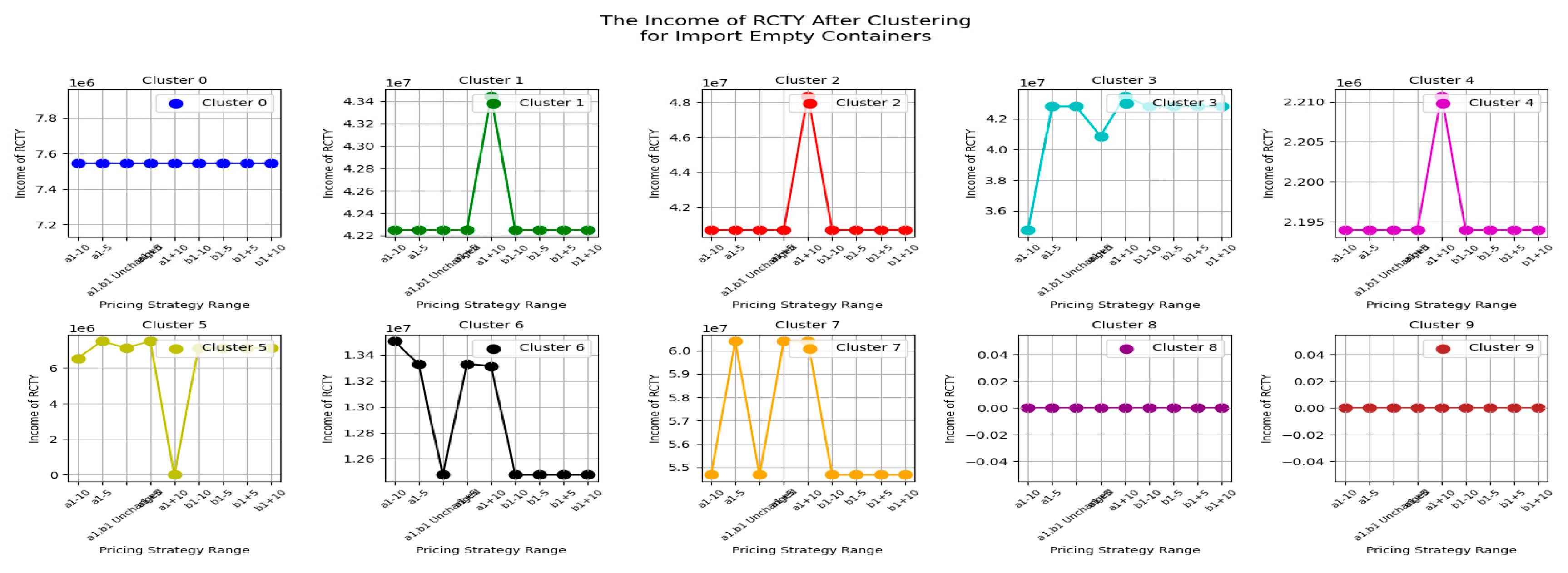
Figure 25.
The carrier’s cost under different pricing strategy scope for import empty containers after the clustering.
Figure 25.
The carrier’s cost under different pricing strategy scope for import empty containers after the clustering.
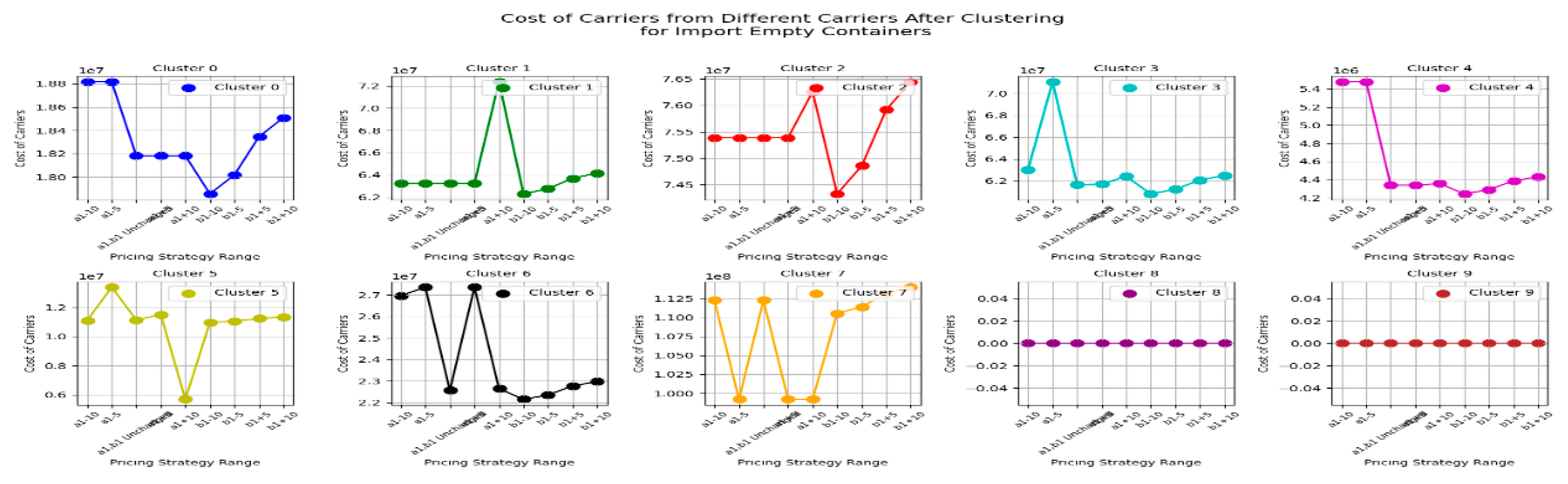
Figure 26.
The carrier’s transfer time under different pricing strategy scope for import empty containers after the clustering.
Figure 26.
The carrier’s transfer time under different pricing strategy scope for import empty containers after the clustering.
After clustering the carriers, the income of CY and the carriers' costs decrease with the expansion of the reduction range and increase with the expansion of the increment range. This trend is consistent with that before clustering. However, the impact of changes in the pricing strategy range on CY's income and carriers' costs varies within each cluster.
Additionally, CY's adjustment of the b1 pricing strategy range does not affect RCTY's income. Similarly, when adjusting the pricing strategy range, the impact on RCTY's income varies due to the characteristics of the carriers within the cluster, resulting in uncertainty. Adjusting the pricing strategy range does not significantly impact carriers' transfer times. Except for a few clusters where an increase of 10 in the pricing strategy range caused significant changes in carriers' transfer time, no changes were observed in other cases.
Therefore, we can draw result 11
Result 11: After clustering import empty containers, adjusting thepricing strategy range consistently influences the income of the port yard and carriers' costs in a predictable manner, while changes in thepricing strategy range introduce variability depending on the characteristics of carriers within each cluster.
The conclusion provide the insight that CY operators, when adjusting the pricing strategy range for b1, should consider not only the changes in their own income but also the impact on the costs for carriers. If CY operators wish to establish a closer cooperative relationship with RCTY, they can simultaneously adjust the pricing strategies of and . By finely tuning , they can achieve a balance between their own revenue and the costs of the carriers; while CY may need to share some of its income with RCTY to strengthen their collaboration.
Next, let's look at the impact of sensitivity changes during the free storage period on the income of CY, the income of RCTY, the cost of the carrier, and the transfer time of the carrier for the import empty container.
From Figure 27, Figure 28, Figure 29 and Figure 30, we can see that for the import empty containers after the clustering, the income of the CY, the carrier's costs and the income of RCTY decrease as the free storage period increases. However, CY's income may fluctuate with the extension of the free storage period, but the overall trend is a decline. In contrast, the carrier's transit time increases with the extension of the free storage period.
Result 12: While longer periods reduce carrier costs and RCTY's income, the fluctuating CY income suggests potential inefficiencies, extending the free storage period also leads to increased carrier transit time.
The result provides the following insights for CY operators to consider potential income changes when setting the free storage period and optimize their free storage period strategy .In addition, CY operators need to weigh the impact of the free storage period on revenue and port operational efficiency, avoiding congestion or resource strain in the yard due to excessively long storage periods. Therefore, CY operators can consider partnering with RCTY to alleviate yard pressure caused by the extension of the free storage period by sharing storage space. This not only helps increase RCTY's income but also expands the available stacking space for CY, optimizing overall operational efficiency.
Similarly, let's take a look at the impact of changes in pricing strategy range and changes in the free storage period on the import shipping containers after the clustering.
From Figure 31 and Figure 33, we can see that for import shipping containers after the clustering, the income of CY and cost of carrier increase with the degree of increase in the pricing strategy range set by CY and decrease with the degree of reduction in the pricing strategy range. From Figure 32 and Figure 34, we can see that RCTY’s income and carrier’s transfer time are not affected by the pricing strategy range set by CY. From this, we derive result 13.
s
So CY's operators may not need to worry too much about the direct effects on their own income when considering the pricing strategy range of . More resources and energy can be invested in other more influential operational strategies. At the same time, the impact of pricing strategy 's range fluctuations is uncertain, which suggests that CY's operators need to be more cautious when formulating or adjusting the range of pricing strategy, which may need to rely on more detailed data analysis and simulations to predict potential impacts under different scenarios. If CY's operators wish to reduce carrier’s costs, they might consider appropriately narrowing the range of the pricing strategy, but they also need to balance other operational metrics that may be affected.
Let's take a look at the impact of changes in the free storage period.
From Figure 35, Figure 36 and Figure 37, we can see that similar to the impact of changes in the free storage period on the income or costs of the three parties after clustering for import empty containers, for import shipping containers after clustering, the income of CY, the income of RCTY, and the carrier's costs decrease as the free storage period increases. In contrast, the carrier's transit time increases as the free storage period extends, which is consistent with the trend observed for clustered import empty containers. From this, we derive result 14.
Result 14: After clustering, both import empty containers and import shipping containers show similar trends.
Result 14 suggests that CY operators should be cautious when setting the free storage period, as a longer free storage period could lead to a decline in income. The extension of the free storage period may also result in lower costs for carriers. This could be beneficial for carriers, but for CY, if it hopes to maintain or increase income, it needs to find a balance that attracts carriers without significantly reducing income.
In general, in this section we explored the impact of the sensitivity of two different container types pricing strategy scope and free storage period sensitivity after the clustering to the income of CY, the income of RCTY, the carrier's cost, and the carrier's transfer time, providing CY managers with some insights into pricing strategies through relevant conclusions.
So far, we have discussed the impact of changes in the range of pricing strategies and the free storage period before and after the clustering. Next, we would like to discuss the differences in solving speed, objective function, and conclusions before and after the clustering.
5.3. Comparison Before and After the Clustering
First, let's take a look at the solution times for each cluster before and after the clustering under different pricing strategy ranges and different free storage periods.
Note: The following abbreviations related to pricing strategy ranges—"-10", "-5", "+5", "+10", "-10", "-5", "+5", "+10"—represent a decrease of 10 in the pricing strategy range for , a decrease of 5 in the pricing strategy range for , an increase of 5 in the pricing strategy range for , an increase of 10 in the pricing strategy range for , a decrease of 10 in the pricing strategy range for , a decrease of 5 in the pricing strategy range for , an increase of 5 in the pricing strategy range for , and an increase of 10 in the pricing strategy range for , respectively.
Significant reduction in overall program running time. Table 5 and Table 6: For import empty containers, the overall running time significantly decreased after clustering. Table 5 shows that the total running time before clustering ranged from 13,094.9 seconds to 14,716.4 seconds, while Table 8 shows that after clustering, this range reduced to 2,054.6 seconds to 2,293.6 seconds. This indicates that the clustering strategy greatly optimized the program's computational efficiency, leading to a substantial reduction in running time. For import shipping containers, a similar reduction in time was observed after clustering. The total running time before clustering ranged from 3,737.01 seconds to 4,458.96 seconds, while after clustering, it decreased to a range of 167.9 seconds to 499.65 seconds.
In addition, equalization of running time across clusters. Import Empty Containers (Table 5 and Table 6): Before clustering, the running time across clusters varied significantly, especially with Cluster 1 and Cluster 2 being much higher than the others. After clustering, these differences significantly decreased. For example, in the a1-10 strategy, the running time for Cluster 1 dropped from 936.83 seconds to 181.15 seconds, making it closer to the other clusters.
Import shipping container (Table 7): Similarly, after clustering, the running time across clusters became more balanced. In Table 7, the running time for Cluster 1 decreased from several thousand seconds to just a few hundred seconds, showing that the clustering strategy helps in more evenly distributing computational resources across different container types.
Next, reduced impact of pricing strategies on running time. Import empty containers (Tables 5and 6): before clustering, different pricing strategy ranges had a significant impact on the running time across clusters, especially for Cluster 2. For example, in Table 5, the running time for Cluster 2 varied by several hundred seconds between the -10 and +10 strategies. After clustering (Table 6), this variation reduced significantly to within a few dozen seconds, indicating that the program's stability improved greatly after clustering. Import shipping containers (Table 7): Similarly, after clustering, the impact of different pricing strategies on each cluster was reduced. For example, under the a1-10 pricing strategy, the running time after clustering was 328.34 seconds, which is a significant reduction compared to before clustering, and it became more stable.
Whether dealing with import empty containers or import shipping containers, the clustering strategy significantly optimized the program's running time, made the running time across clusters more balanced, and reduced the impact of pricing strategies on the program's stability.
Considering Tables 5, 6, and 7, the clustering strategy has shown excellent performance in enhancing computational efficiency, balancing computational load, and reducing the impact of pricing strategies on running time. This is crucial for maintaining efficient and stable system operation in complex operational environments.
A comparative analysis of the data presented in Table 8 and Table 9 elucidates the substantial impact of clustering on program running times for import empty container. The comparison of import empty container clustering before and after clustering shows that the clustering scheme effectively reduces operating time in most cases, especially when the free storage period is shorter. The data after clustering indicates that the operating time of most clusters has significantly decreased, optimizing the overall system efficiency. For example, clusters such as Cluster 0, Cluster 1, and Cluster 2 show the most noticeable reduction in operating time when the free storage period is shorter, suggesting that the clustering scheme effectively improves the pricing efficiency of carriers within these clusters.

Table 9.
Operating Time of Different Free Storage Period for Each Cluster After Clustering of Import Empty Container.
Table 9.
Operating Time of Different Free Storage Period for Each Cluster After Clustering of Import Empty Container.
| After the Clustering | ||||||||
|---|---|---|---|---|---|---|---|---|
| Free Storage Period | 5 | 6 | 7 | 8 | 9 | 10 | 11 | 12 |
| Cluster 0 | 152.33 | 175.50 | 182.14 | 221.13 | 221.64 | 212.00 | 212.18 | 117.01 |
| Cluster 1 | 153.66 | 162.50 | 155.43 | 195.00 | 189.90 | 184.20 | 176.47 | 96.01 |
| Cluster 2 | 393.40 | 390.65 | 428.99 | 462.57 | 483.23 | 436.30 | 433.41 | 272.49 |
| Cluster 3 | 430.48 | 465.57 | 450.70 | 457.73 | 437.26 | 415.67 | 418.92 | 266.71 |
| Cluster 4 | 195.38 | 89.74 | 100.19 | 185.49 | 164.04 | 159.41 | 149.17 | 126.96 |
| Cluster 5 | 110.46 | 242.06 | 290.37 | 112.05 | 106.48 | 105.41 | 240.78 | 233.28 |
| Cluster 6 | 264.20 | 300.37 | 368.24 | 267.23 | 252.09 | 231.17 | 205.36 | 211.09 |
| Cluster 7 | 401.64 | 464.56 | 505.51 | 322.94 | 320.67 | 267.87 | 104.84 | 115.85 |
| Cluster 8 | 0.42 | 0.54 | 9.28 | 7.79 | 7.24 | 6.08 | 5.87 | 6.29 |
| Cluster 9 | 11.13 | 13.89 | 26.65 | 7.41 | 7.53 | 6.39 | 6.19 | 7.26 |
| Total | 2113.1 | 2305.4 | 2517.5 | 2239.4 | 2190.1 | 2024.5 | 1953.2 | 1453.0 |
Table 10.
Operating Time of Different Free Storage Period for Each Cluster Before Clustering of Import Shipping Container.
Table 10.
Operating Time of Different Free Storage Period for Each Cluster Before Clustering of Import Shipping Container.
| Before the Clustering | ||||||||
|---|---|---|---|---|---|---|---|---|
| Free Storage Period | 5 | 6 | 7 | 8 | 9 | 10 | 11 | 12 |
| Cluster 0 | 2271.23 | 1681.73 | 2164.47 | 1770.07 | 1741.59 | 1647.96 | 1614.07 | 1863.95 |
| Cluster 1 | 2856.62 | 2223.96 | 2784.71 | 2342.78 | 2318.17 | 2278.03 | 2231.8 | 2566.51 |
| Cluster 2 | 69.54 | 98.97 | 70.83 | 68.69 | 71.37 | 70.47 | 72.49 | 73.15 |
| Cluster 3 | 102.27 | 78.78 | 99.97 | 91.18 | 89.83 | 86.03 | 85.73 | 88.64 |
| Total | 5299.66 | 4083.44 | 5119.98 | 4272.72 | 4220.96 | 4082.49 | 4004.09 | 4592.25 |
Table 11.
Operating Time of Different Free Storage Period for Each Cluster After Clustering of Import Shipping Container.
Table 11.
Operating Time of Different Free Storage Period for Each Cluster After Clustering of Import Shipping Container.
| After the Clustering | ||||||||
|---|---|---|---|---|---|---|---|---|
| Free Storage Period | 5 | 6 | 7 | 8 | 9 | 10 | 11 | 12 |
| Cluster 0 | 68.87 | 87.83 | 96.93 | 122.45 | 103.74 | 100.73 | 99.36 | 60.77 |
| Cluster 1 | 163.94 | 182.10 | 180.10 | 221.91 | 211.06 | 207.62 | 198.55 | 128.03 |
| Cluster 2 | 96.35 | 98.17 | 99.07 | 133.62 | 132.65 | 126.50 | 124.42 | 83.09 |
| Cluster 3 | 18.76 | 18.45 | 18.11 | 21.66 | 20.39 | 20.33 | 20.05 | 12.57 |
| Total | 347.91 | 386.54 | 394.21 | 499.65 | 467.83 | 455.18 | 442.38 | 284.46 |
However, although most clusters benefit from clustering, a few clusters, such as Cluster 8 and Cluster 9, show an increase in operating time after clustering, particularly when the free storage period is longer. This phenomenon is more pronounced, but fortunately, the pricing running time for these two clusters does not show significant deviation, which is within an acceptable range.
A comparative analysis of the data presented in Table 8 and Table 9 for import shipping container. The clustering of import shipping containers has significantly reduced operating times across the board, with particularly strong improvements seen in clusters with initially higher operating times. This indicates that the clustering scheme effectively optimizes the management of import heavy containers, improving overall operational efficiency. Even clusters that showed less dramatic changes still benefited from reduced operating times, suggesting that the clustering process is broadly effective.
Overall, clustering has a noticeable optimization effect on operating time, especially when the free storage period is shorter. The operating time of most clusters has significantly decreased, leading to a marked improvement in the pricing efficiency of CY. For import empty containers, running times before clustering varied significantly across clusters, with some clusters, such as Cluster 1 and Cluster 2, exhibiting considerably higher time. Post-clustering, running times across clusters became more uniform, with a general reduction observed; for example, Cluster 1's time decreased from 881.91 seconds to 195.00 seconds. Likewise, for import shipping containers, there was a notable variation in running times across clusters before clustering, particularly in Cluster 0 and Cluster 1. After clustering, running times became more balanced, with substantial reductions across all clusters, such as Cluster 0's time dropping from 1,770.07 seconds to 122.45 seconds. This analysis indicates that clustering effectively reduces discrepancies in running times across clusters and optimizes performance stability, regardless of the container type or storage period.
Analyzing Figure 39, Figure 40 and Figure 41 before and after clustering for different pricing strategy ranges of import empty containers, we can observe that for import empty containers, the clustering of carriers by CY (Container Yard) for pricing leads to a decrease in CY's overall income, while the income for RCTY (Regional Container Transfer Yard) increases, and the storage costs for carriers rise. Therefore, port operators may consider using the pricing strategy based on carrier clustering to negotiate with RCTY for cooperation. This approach could not only improve the pricing efficiency of CY towards carriers but also enhance the utilization of storage space within the yard by collaborating with RCTY, thereby improving the operational efficiency of the yard within the port.
From the perspective of different clusters, clustering has had varying impacts on pricing. Taking Cluster 1 as an example, the pricing after clustering significantly increased the terminal yard revenue, especially under the +10 strategy, where the revenue rose from 35,068,780.37 to 20,250,708.62, demonstrating that the post-clustering pricing strategy effectively enhanced the revenue generated from cluster carriers at the terminal yard. In contrast, the pricing strategies for Cluster 0 and Cluster 3 led to a decrease in terminal yard revenue, especially under the -10 and +10 strategies, where revenue dropped from 7,723,415.80 and 23,508,019.68 to 8,252,695.16 and 20,762,119.15, respectively. This suggests that the optimization effect of clustering on these clusters is not as significant as on others.
Overall, clustering, through different pricing strategies, has increased the CY’s income of most clusters. Although some clusters experienced a decrease in CY’s income under certain strategies, clustering generally enhances the overall pricing efficiency by refining pricing strategies. Moreover, the change in CY income is directly associated with the pricing strategy. An increase in the pricing strategy range typically leads to higher cluster CY’s income, especially under higher pricing strategies range, where CY's income grows more significantly. However, different clusters react differently, and the income growth of some clusters' CY may be limited. Therefore, more precise pricing strategies need to be developed based on the characteristics of each cluster.
From the perspective of RCTY Income, before clustering, there was a significant variation in RCTY Income across different pricing strategies. For example, the RCTY Income for Cluster 1 was 24,017,177.55 under the a1-10 strategy, but it dropped to 9,008,367.32 under the +10 strategy. This suggests that for some clusters (such as Cluster 1), RCTY Income remains relatively stable under certain pricing strategy ranges, but it can decrease significantly under other pricing strategy ranges. A similar trend can be observed in other clusters, particularly in Cluster 0, Cluster 2, and Cluster 3, where the Income fluctuates considerably under different pricing strategy ranges. After clustering, the adjustment of pricing strategy ranges significantly improved RCTY Income for most clusters, especially for Cluster 1 and Cluster 3. For instance, under the +10 strategy, Cluster 1’s income increased from 9,008,367.32 to 43,448,855.98, indicating that the post-clustering pricing strategy significantly enhanced the RCTY Income for this cluster.
From the perspective of carriers’ cost, the data before and after clustering indicates significant differences in the impact of CY's pricing strategy ranges on carrier costs. Before clustering, some clusters (such as Cluster 1 and Cluster 3) showed considerable cost fluctuations under different pricing strategies. For example, Cluster 1 had a carrier cost of 48,276,534.77 under the -10 strategy, which decreased to 46,125,203.99 under the +10 strategy, demonstrating sensitivity to the pricing strategy. After clustering, the cost volatility of many clusters decreased, particularly for Cluster 1 and Cluster 7, indicating that optimizing the pricing strategy can effectively stabilize carrier costs. Specifically, after clustering, the cost for Cluster 1 fluctuated between 62,288,807.97 and 72,354,924.14 under the -10, +5, and +10 strategies, reflecting improved stability in pricing strategies post-clustering. However, it is important to note that while stability increased, the overall costs for certain clusters (such as Cluster 1 and Cluster 7) increased, especially under the +10 strategy.
Therefore, the analysis before and after clustering indicates that CY needs to develop different pricing strategies for different clusters to reduce cost fluctuations and optimize carrier cost control. By refining and differentiating the pricing strategy, CY income can be maximized across different clusters, and the pricing range can be flexibly adjusted based on the characteristics and demand fluctuations of each cluster. High pricing strategies have significant potential to increase revenue in clusters with higher demand and stronger capacity, while clusters with lower demand should avoid excessively high pricing to maintain revenue stability. Ultimately, through continuous dynamic adjustments and regular optimization, CY can improve overall operational efficiency and income.
Next, let's look at the changes in the income/cost of the third party for import shipping containers before and after clustering, under different pricing strategy ranges set by CY.
Analyzing Figure 42, Figure 43 and Figure 44 before and after clustering for different pricing strategy ranges of import shipping containers, CY income in Cluster 0 showed a decline with wider pricing strategy ranges, while Cluster 1 remained relatively stable but still saw a slight decrease when the pricing range increased. Cluster 2 exhibited substantial fluctuations, particularly with larger pricing strategy ranges, leading to a notable decrease in CY income. Cluster 3's income remained lower and stable. After clustering, Cluster 0's CY income improved, especially with reduced pricing ranges, while Cluster 1 showed reduced fluctuations and maintained higher income. Cluster 2 saw an increase in CY income, especially under narrower pricing ranges. Cluster 3 showed minimal changes.
For RCTY income, before clustering, Cluster 0 had stable income, especially with wider pricing ranges. Cluster 1 maintained a high and stable income but decreased slightly with reduced ranges. Cluster 2 showed greater fluctuations, especially with expanded pricing ranges. After clustering, Cluster 0's RCTY income increased with smaller pricing ranges, while Cluster 1 showed fluctuations but generally maintained a high level. Cluster 2’s income rose, particularly under -10 and , unchange strategies. Cluster 3's income remained stable.
Regarding carrier costs, before clustering, Cluster 0 showed a slight decrease as the pricing strategy range expanded, while Cluster 1 experienced consistently high costs. Cluster 2 showed volatility, and Cluster 3 had the lowest and most stable costs. After clustering, Cluster 0's carrier costs increased with narrower pricing ranges. Cluster 1 saw more variation, and Cluster 2's costs increased, particularly with certain strategies. Cluster 3’s costs remained stable.
The analysis suggests that clustering helps in identifying distinct cost and income patterns within clusters, allowing port operators to optimize pricing strategies. By using differentiated pricing strategies, especially for clusters with more volatility, operators can reduce income fluctuations and better manage carrier costs, leading to more stable and optimized revenue streams.
Analyzing Figure 45, Figure 46 and Figure 47 before and after clustering for different free storage periods of import empty containers, the changes in CY Income under different free storage periods before and after clustering indicate that clustering optimized the income performance across clusters. Before clustering, different clusters showed significant differences in response to changes in the free storage period, especially Cluster 0 and Cluster 2, where income decreased as the free storage period increased, demonstrating sensitivity to the free storage period. After clustering, the income fluctuations across clusters were significantly reduced, particularly under shorter free storage periods, with improved income performance and greater stability. For example, Cluster 0 and Cluster 2 saw a notable increase in income under shorter free storage periods, while Cluster 1 showed higher income stability.
The changes in RCTY income before and after clustering under different free storage periods indicate that clustering optimized the RCTY income performance between clusters, particularly reducing the volatility of RCTY income when the free storage period was shorter. Before clustering, different clusters showed a strong sensitivity to changes in the free storage period, especially Cluster 0 and Cluster 2, where RCTY income exhibited a significant decline during longer free storage periods, showing greater volatility. After clustering, the volatility of RCTY income across clusters significantly decreased, particularly in shorter free storage periods, with improved performance across multiple clusters, demonstrating stronger stability. For instance, RCTY income for Cluster 0 and Cluster 2 increased noticeably during shorter free storage periods, while Cluster 1 exhibited higher stability. Overall, after clustering, the fluctuation of RCTY income was reduced, especially for longer free storage periods, with RCTY income becoming more stable within clusters. This suggests that clustering optimization helps improve the stability of RCTY income and reduces the negative impact of the free storage period on RCTY income.
The changes in carrier costs under different free storage periods before and after clustering indicate that clustering optimized the carrier cost performance across clusters, particularly reducing the volatility of carrier costs when the free storage period is shorter. Before clustering, the carrier costs across clusters exhibited greater fluctuations, especially in Cluster 0, Cluster 1, and Cluster 7, where there was a significant downward trend in carrier costs with longer free storage periods, showing considerable volatility. After clustering, the fluctuations in carrier costs across clusters were significantly reduced, with multiple clusters exhibiting more stable carrier costs, particularly when the free storage period was shorter. For instance, Cluster 0 and Cluster 2 showed an increase in carrier costs during shorter free storage periods, while Cluster 1 demonstrated higher stability, with much less volatility in carrier costs. Overall, clustering resulted in more stable carrier costs, especially when the free storage period was longer, with costs tending to stabilize across clusters.
Overall, clustering optimized CY income, particularly when the free storage period was shorter, with significant improvements in the performance of CY income across multiple clusters, showing higher stability. Compared to before clustering, the fluctuations in CY income were notably reduced, especially when the free storage period was longer, and after clustering, CY income tended to stabilize. This suggests that the clustering method effectively balances CY income across different clusters under varying free storage periods, reducing excessive fluctuations in CY income. This change may stem from optimized resource allocation within the clusters, enhancing the overall stability of CY income and strengthening the system's resilience to the impact of free storage period variations on CY income.
Analyzing Figure 48, Figure 49 and Figure 50 before and after clustering for different free storage periods of import shipping containers, clustering optimized the CY income performance of each cluster, especially for shorter free storage periods, where the CY income of multiple clusters showed significant improvement. Before clustering, the CY income fluctuated greatly, particularly for longer free storage periods, where the CY income of multiple clusters showed a downward trend with high volatility. After clustering, the fluctuations in CY income were significantly reduced, especially for shorter free storage periods, where multiple clusters became more stable. For example, Cluster 0 and Cluster 1 showed a significant increase in CY income for shorter free storage periods, while Cluster 2 and Cluster 3 exhibited higher stability.
RCTY income saw significant improvement in multiple clusters, especially during shorter free storage periods. Before clustering, RCTY income fluctuated greatly, particularly during longer free storage periods, with a downward trend in several clusters. After clustering, the fluctuations in RCTY income were significantly reduced, especially during shorter free storage periods, where multiple clusters became more stable. For example, Cluster 0 and Cluster 1 saw a significant increase in RCTY income during shorter free storage periods, while Cluster 2 and Cluster 3 showed more stable income performance.
Additionally, before clustering, the carrier costs varied significantly across clusters, especially during longer free storage periods, where the carrier costs of multiple clusters showed different trends. After clustering, the carrier costs became smoother across clusters, with notable optimization, especially during shorter free storage periods. For example, the carrier costs of Cluster 0 and Cluster 1 increased during shorter free storage periods, while Cluster 2 and Cluster 3 maintained a more consistent downward trend.
These analyses provide important insights for port operators. First, shorter free storage periods significantly improved CY and RCTY income across multiple clusters, especially after clustering optimization, where income volatility was greatly reduced. Port operators can adjust free storage period strategies based on cluster characteristics to optimize storage management and improve income stability. Additionally, clustering optimized carrier costs, particularly during shorter free storage periods, where carrier costs across multiple clusters were effectively controlled. Based on these insights, port operators should consider differentiated pricing strategies, increasing charges for better-performing clusters, while optimizing free storage period settings for others. Furthermore, ports can achieve more efficient resource allocation through refined operational management, stabilizing income and enhancing overall operational efficiency and competitiveness.
6. Conclusion and Recommendations
This study emphasizes the critical role of port pricing strategies in the effective coordination among CY, RCTY, and carriers. By employing mixed clustering techniques and conducting comprehensive sensitivity analyses, it provides insights into how different pricing models and strategies impact the solution time and results of port pricing outcomes, offering valuable perspectives to CY operators through the conclusions drawn.
The analysis reveals that pricing strategies and their adjustments have a significant impact on the revenue and cost of CY, RCTY, and carriers. The identification of diverse responses to pricing strategies across different clusters highlights the need for tailored approaches that address the specific characteristics and demands of each market segment. A key contribution of this study is the understanding of how carrier layered pricing affects the objective functions of system participants in the port pricing environment. The findings underscore the importance of dynamic pricing models and collaborative strategies to mitigate adverse effects.
Overall, this research provides actionable recommendations for port operators, including strategic adjustments to pricing models and enhanced collaboration with RCTY. Additionally, it lays the groundwork for future research, suggesting areas for further exploration to refine and expand the understanding of port pricing strategies in diverse contexts.
Future research can expand in several directions to further enhance the optimization and understanding of port pricing strategies. First, multi-port analysis should be a key focus, with future studies considering expansion to other ports to verify and compare the universality of pricing strategies and clustering effects across different port environments. This will help in understanding the impact of different geographic regions and market conditions on pricing models. Second, exploring additional clustering methods is also a valuable area of research. Researchers could try alternative clustering algorithms, such as hierarchical or density-based clustering, to identify methods better suited to specific datasets. This may reveal more granular group characteristics and opportunities for optimizing pricing strategies.
Furthermore, future studies should emphasize data diversity, considering the use of larger and higher-quality datasets to enhance the reliability and general applicability of findings. This includes obtaining information from more ports and different types of transportation data. Finally, expanding sensitivity analysis is also an important research direction. Further extending the scope of sensitivity analysis to explore system responses under various pricing strategy combinations and conditions will help reveal the performance and stability of strategies in different scenarios. These research directions will provide a more comprehensive perspective and solutions for optimizing port pricing strategies, advancing the field of port management.
References
- 陈喜燕. 零堆存费对航运市场发展的危害. 集装箱化 2016, 27, 25–26.
- Lee, C.-Y. & Yu, M. Inbound container storage price competition between the container terminal and a remote container yard. Inbound container storage price competition between the container terminal and a remote container yard. Flex. Serv. Manuf. J. 2012, 24, 320–348. [Google Scholar]
- Cui, H. & Notteboom, T. A game theoretical approach to the effects of port objective orientation and service differentiation on port authorities’ willingness to cooperate. Res. Transp. Bus. Manag.
- 施欣. 港口服务产品差异化策略竞争博弈对策分析. in 中国航海学会2001年度学术交流会论文集 5 (中国航海学会, 2001).
- Yu, M. , Tian, X., & IEEE. Ocean Carrier’s Free-time Pricing Scheme for Inbound Container Storage. in 130–134 (2014). [CrossRef]
- 王盛华. 基于博弈论的港口公路运输服务整合及定价策略研究. (大连理工大学, 2019).
- Wang, H. , Ruan, Y., Niu, B. & Zhang, H. Intra-port demand coordination and inter-port competition: Ports’ pricing strategies with congestion concerns. OCEAN Coast. Manag. 2024, 248, 106918. [Google Scholar]
- Ma, Y. , Johnson, D., Wang, J. Y. T. & Shi, X. Competition for rail transport services in duopoly market: Case study of China Railway(CR) Express in Chengdu and Chongqing. Res. Transp. Bus. Manag. 0052. [Google Scholar]
- Yuan, K. , Wang, X. & Zhang, Q. Inter-Port Competition and Cooperation Under Different Market Environments. Transp. Res. Rec. 2022, 2676, 2676, 643–659. [Google Scholar]
- Zhang, Q. , Wang, W., Peng, Y., Zhang, J. & Guo, Z. A game-theoretical model of port competition on intermodal network and pricing strategy. Transp. Res. PART E-Logist. Transp. Rev.
- 杨姝文. 考虑班轮公司的两阶段集装箱堆存定价研究. (大连海事大学, 2020). [CrossRef]
- Dong, G. & Huang, R. Inter-port price competition in a multi-port gateway region. Res. Transp. Econ. 2022, 94, 101178. [Google Scholar]
- Woo, Y. J. , Song, J.-H. & Kim, K. H. Pricing storage of outbound containers in container terminals. H. Pricing storage of outbound containers in container terminals. Flex. Serv. Manuf. J. 2016, 28, 644–668. [Google Scholar]
- Xing, W. , Liu, Q. & Chen, G. Pricing strategies for port competition and cooperation. Pricing strategies for port competition and cooperation. Marit. POLICY Manag. 2018, 45, 260–277. [Google Scholar]
- Dong, G. & Zhong, D. Tacit Collusion of Pricing Strategy Game between Regional Ports: The Case of Yangtze River Economic Belt. SUSTAINABILITY.
- 孙赫迎 & 曾庆成. 考虑码头内外堆场竞争的集装箱堆存定价模型. 运筹与管理 28, 145–151 (2019).
- 杨姝文, 曾庆成 & 于婷. 堆存需求变动的集装箱码头内外部堆场定价模型. 中国水运(下半月) 19, 82-83+151 (2019).
- Giat, Y. Storage Fees in a Container Yard with Multiple Customer Types. Proceedings OF THE 10TH INTERNATIONAL CONFERENCE ON OPERATIONS RESEARCH AND ENTERPRISE SYSTEMS (ICORES) (eds. Parlier, G. H., Liberatore, F. & Demange, Setubal, 2021)., M.) 177–184 (Scitepress. [CrossRef]
- Kim, K. H. & Kim, K. Y. Optimal price schedules for storage of inbound containers. Transp. Res. PART B-Methodol.
- Martin, E. , Salvador, J. & Sauri, S. Storage pricing strategies for import container terminals under stochastic conditions. Transp. Res. PART E-Logist. Transp. Rev.
- Wen, D. , Xiao, T. & Dastani, M. Pricing strategy and collection rate for a supply chain considering environmental responsibility behaviors and rationality degree. Pricing strategy and collection rate for a supply chain considering environmental responsibility behaviors and rationality degree. Comput. Ind. Eng. 2022, 169, 108290. [Google Scholar]
- He, S. & Ma, Z. Service quality and price competition in crowdsourced delivery markets. Service quality and price competition in crowdsourced delivery markets. Int. Trans. Oper. Res. 2024, 31, 2023–2055. [Google Scholar]
- Jiang, L. , Wang, X., Yang, K. & Gao, Y. Collaborative optimization of acquisition selection and service pricing for inland-river ports based on repeated games. Eng. Optim.
- Hong-Oanh Nguyen, Chin, A., Tongzon, J. & Bandara, M. Analysis of strategic pricing in the port sector: The network approach. Marit. Econ. Logist.
Figure 1.
Average Port Waiting Time for Container Ships.
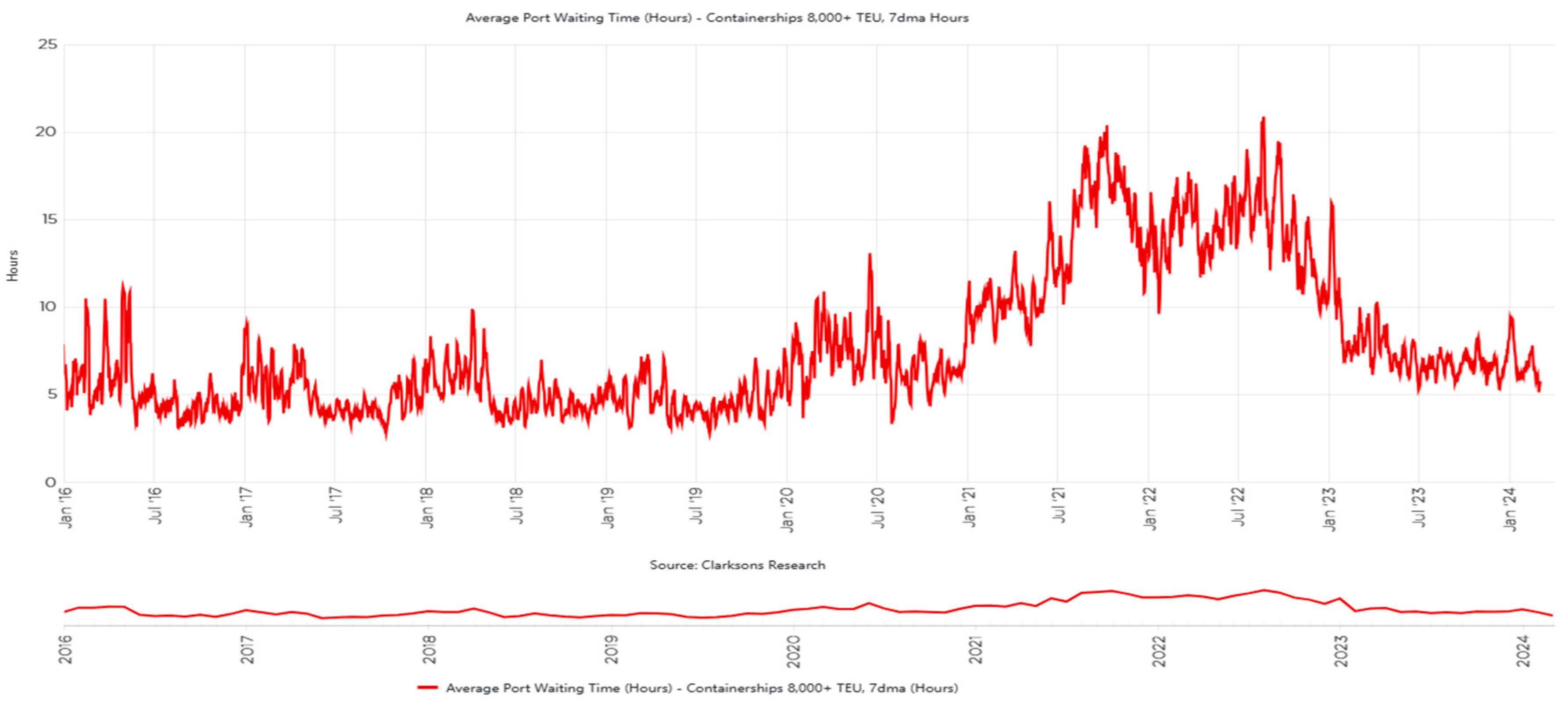
Figure 2.
A specific description of a three-party game.
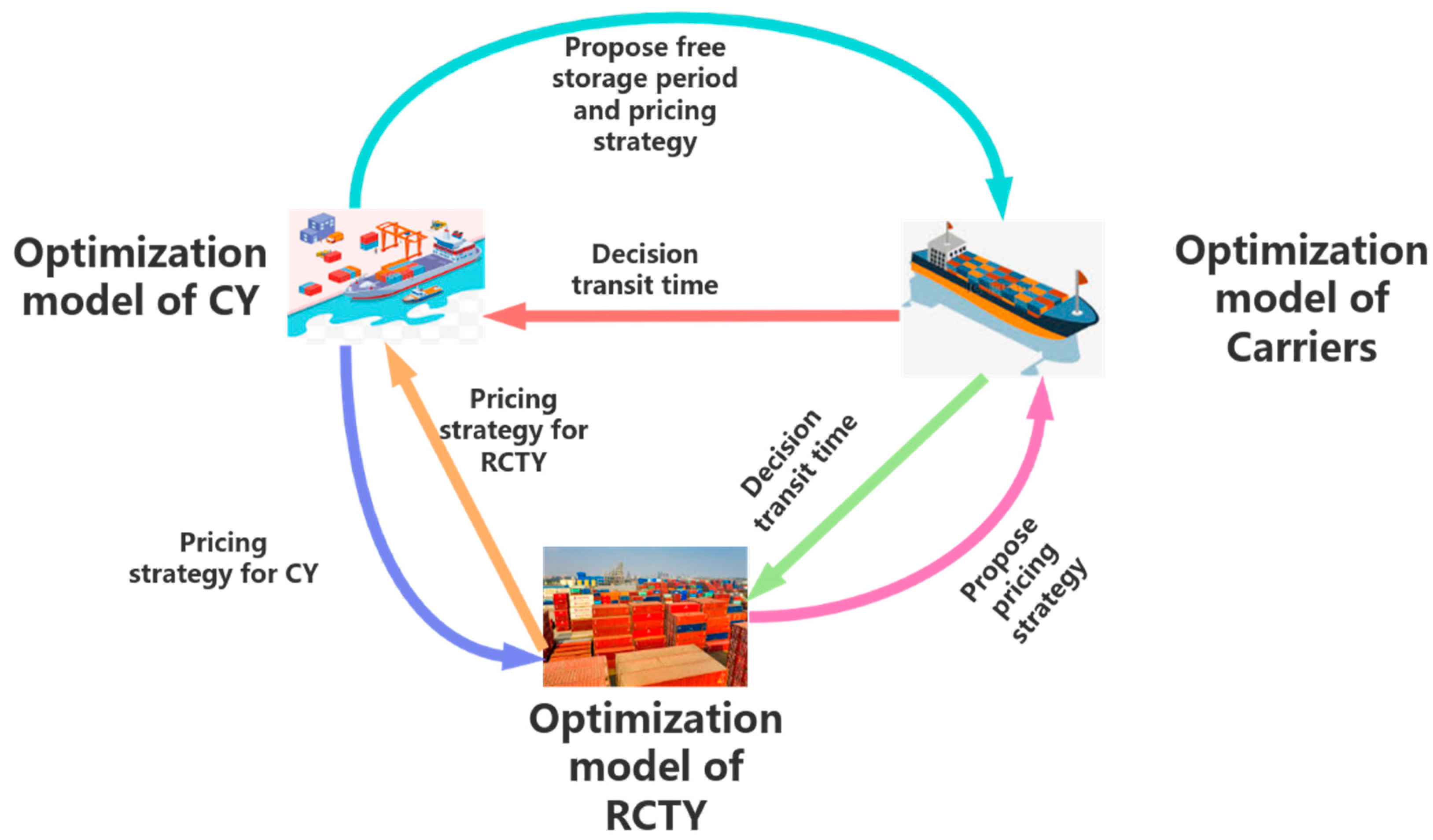
Figure 3.
Histogram of the dwell time of import shipping containers from different carriers at a port in Southeast China.
Figure 3.
Histogram of the dwell time of import shipping containers from different carriers at a port in Southeast China.

Figure 4.
Histogram of the dwell time of import empty containers from different carriers at a port in Southeast China.
Figure 4.
Histogram of the dwell time of import empty containers from different carriers at a port in Southeast China.
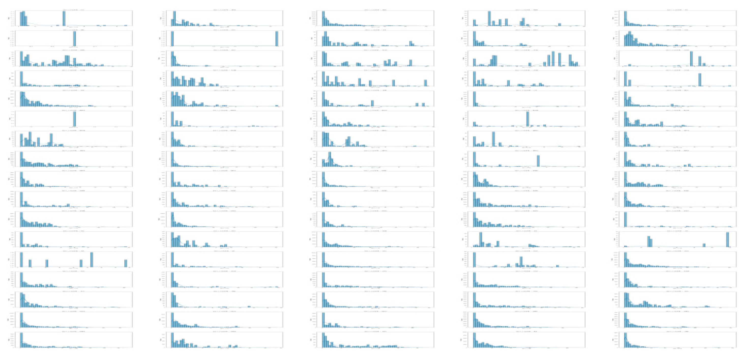
Figure 5.
Clustering Results for Import Shipping Containers with Various Carriers.
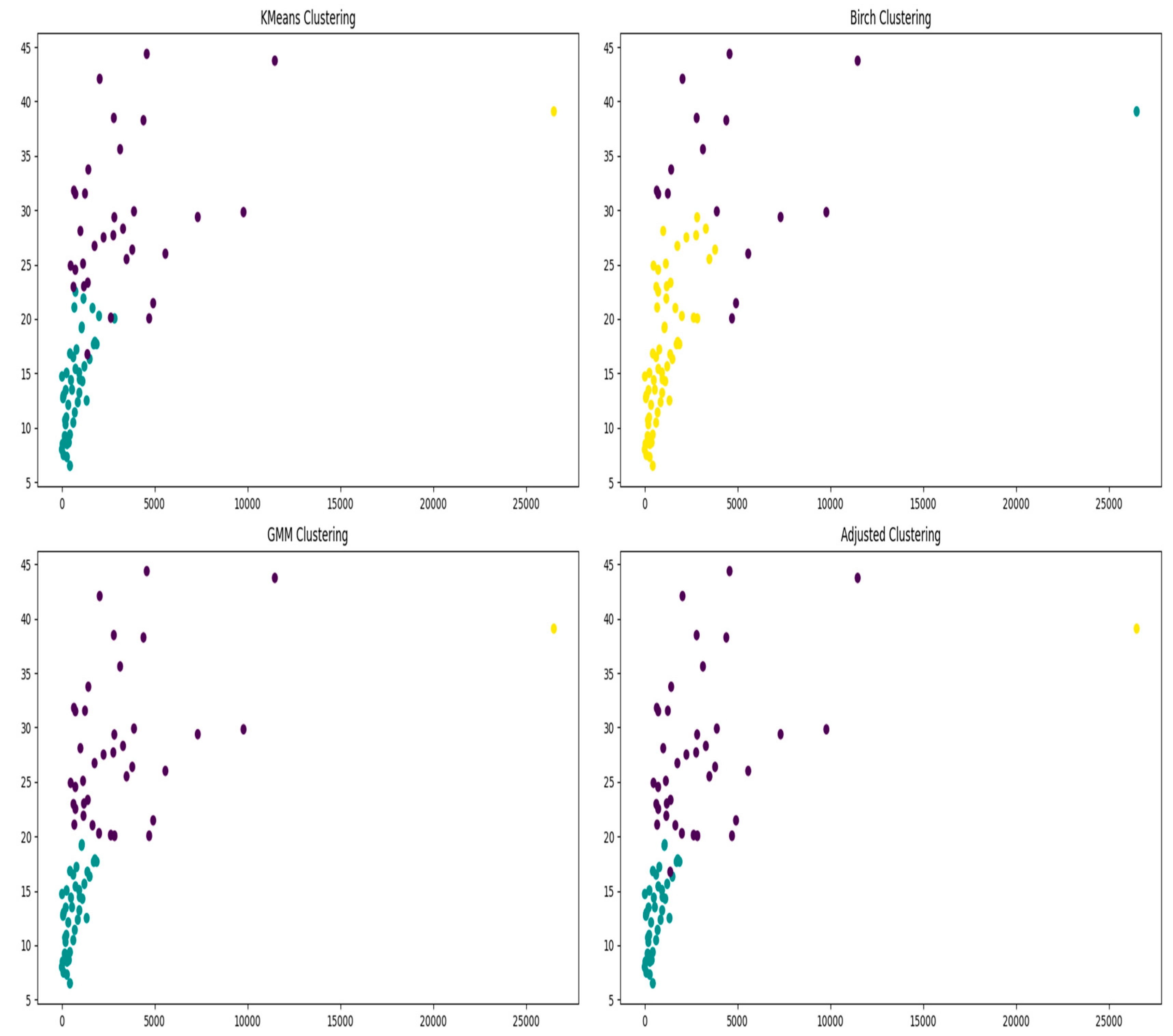
Figure 6.
Clustering Results for Import Empty Containers with Various Carriers.
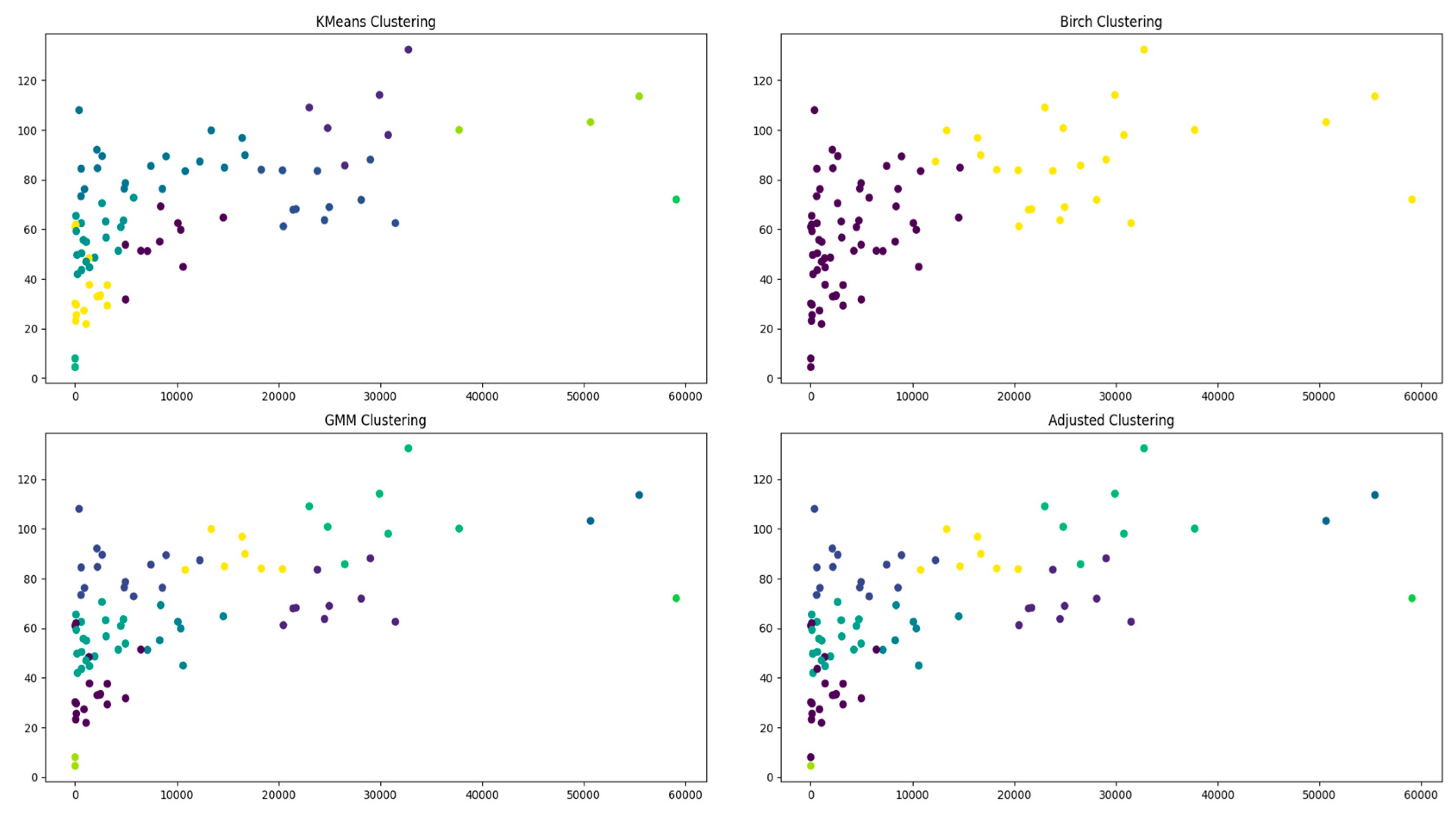
Figure 7.
The changes in the CY’s income under different pricing strategies for import empty containers before the clustering.
Figure 7.
The changes in the CY’s income under different pricing strategies for import empty containers before the clustering.
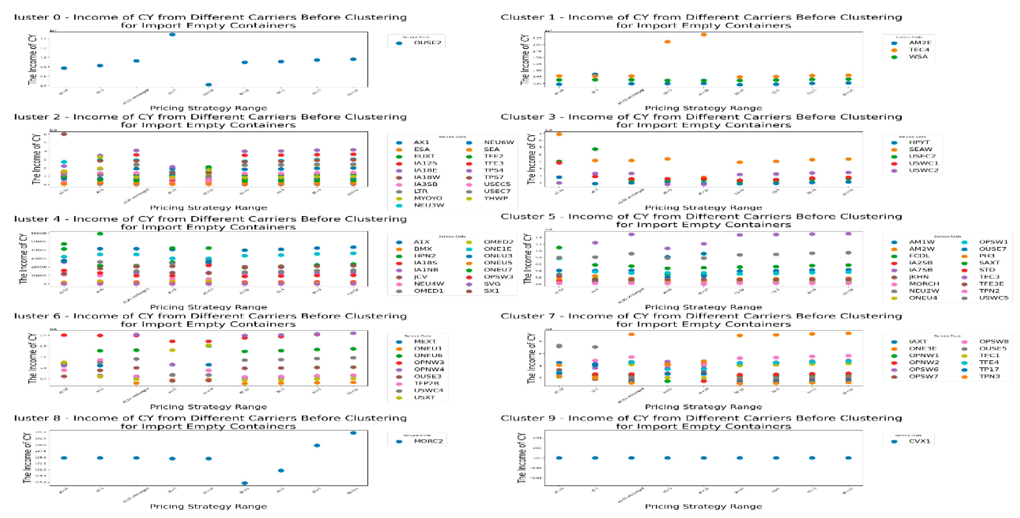
Figure 8.
The RCTY’s income under different pricing strategies for import empty containers before the clustering.
Figure 8.
The RCTY’s income under different pricing strategies for import empty containers before the clustering.
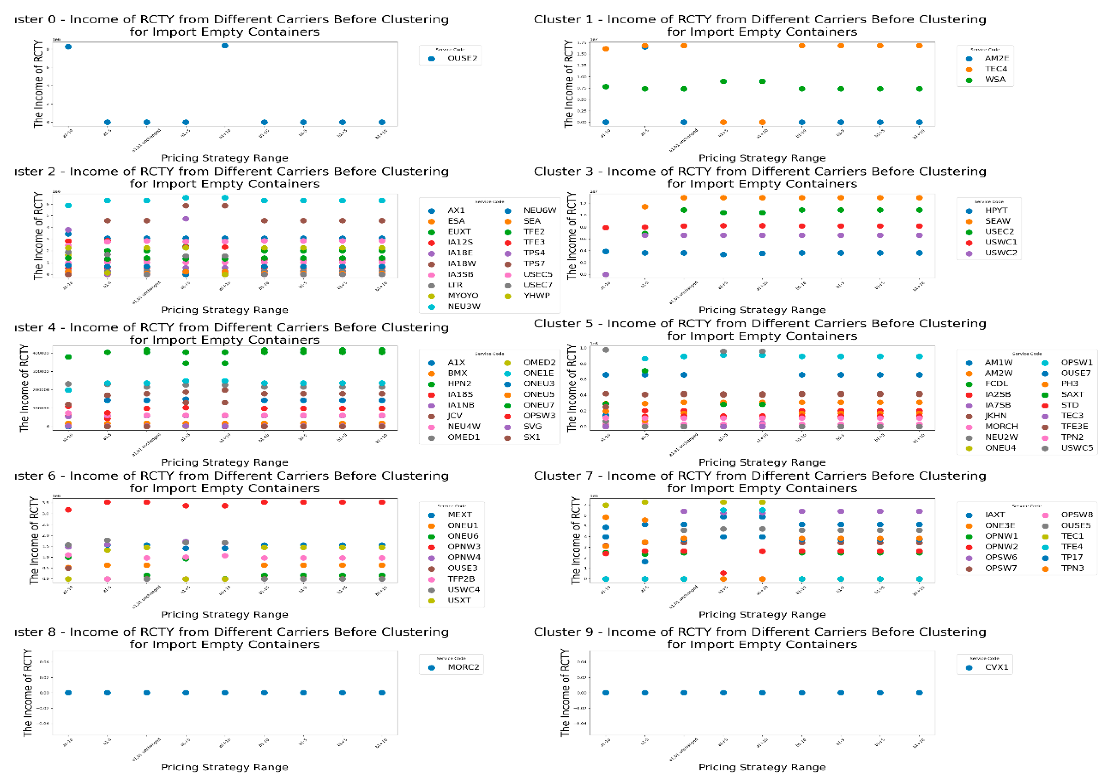
Figure 9.
The carrier’s costs under CY’s different pricing strategies range for import empty containers before the clustering.
Figure 9.
The carrier’s costs under CY’s different pricing strategies range for import empty containers before the clustering.
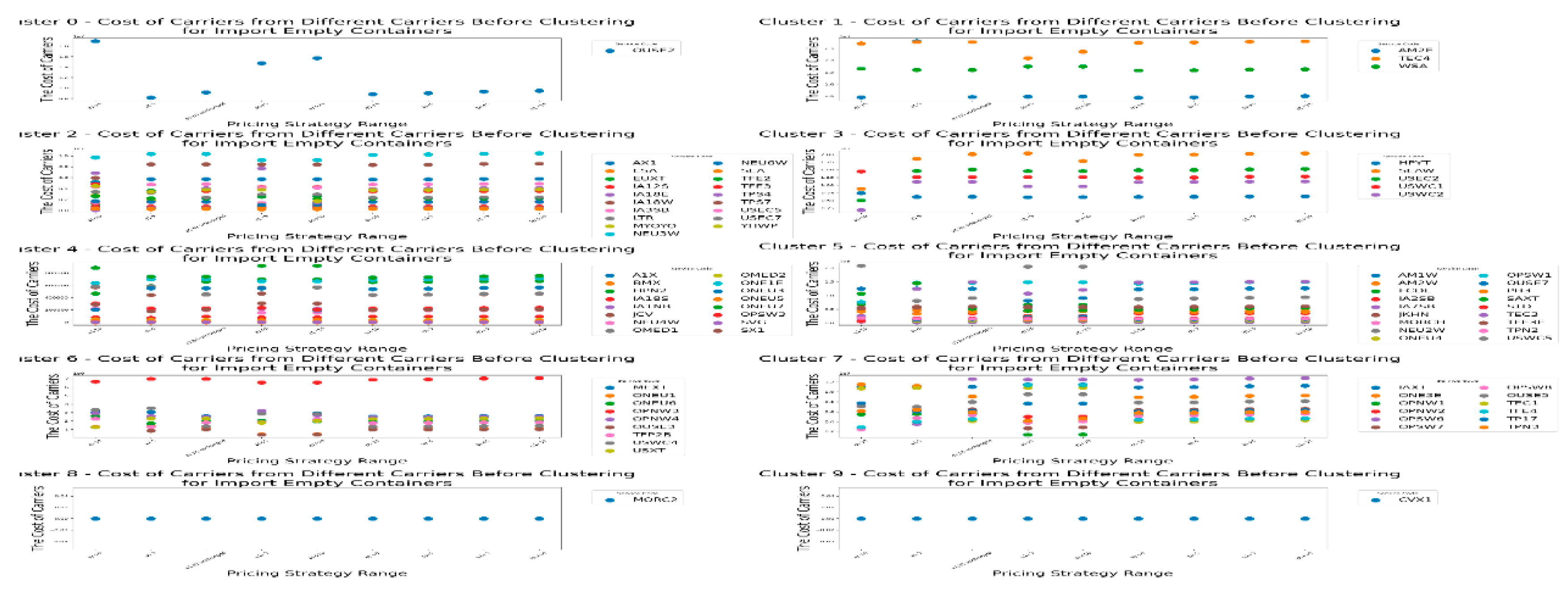
Figure 10.
The carrier’s transfer time under CY’s different pricing strategies for import empty containers before the clustering.
Figure 10.
The carrier’s transfer time under CY’s different pricing strategies for import empty containers before the clustering.
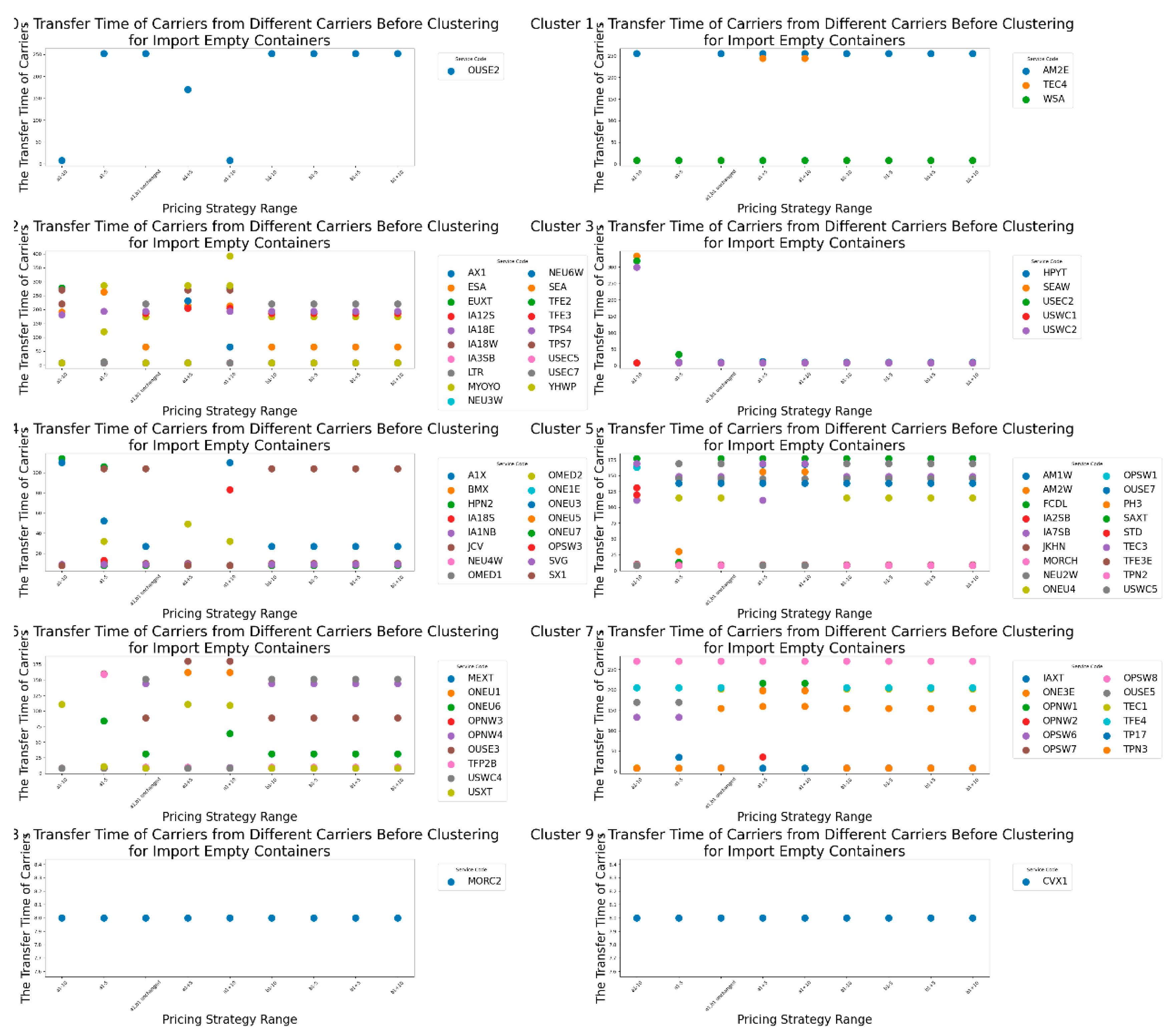
Figure 11.
The CY’s income under different free storage period for import empty containers before the clustering.
Figure 11.
The CY’s income under different free storage period for import empty containers before the clustering.
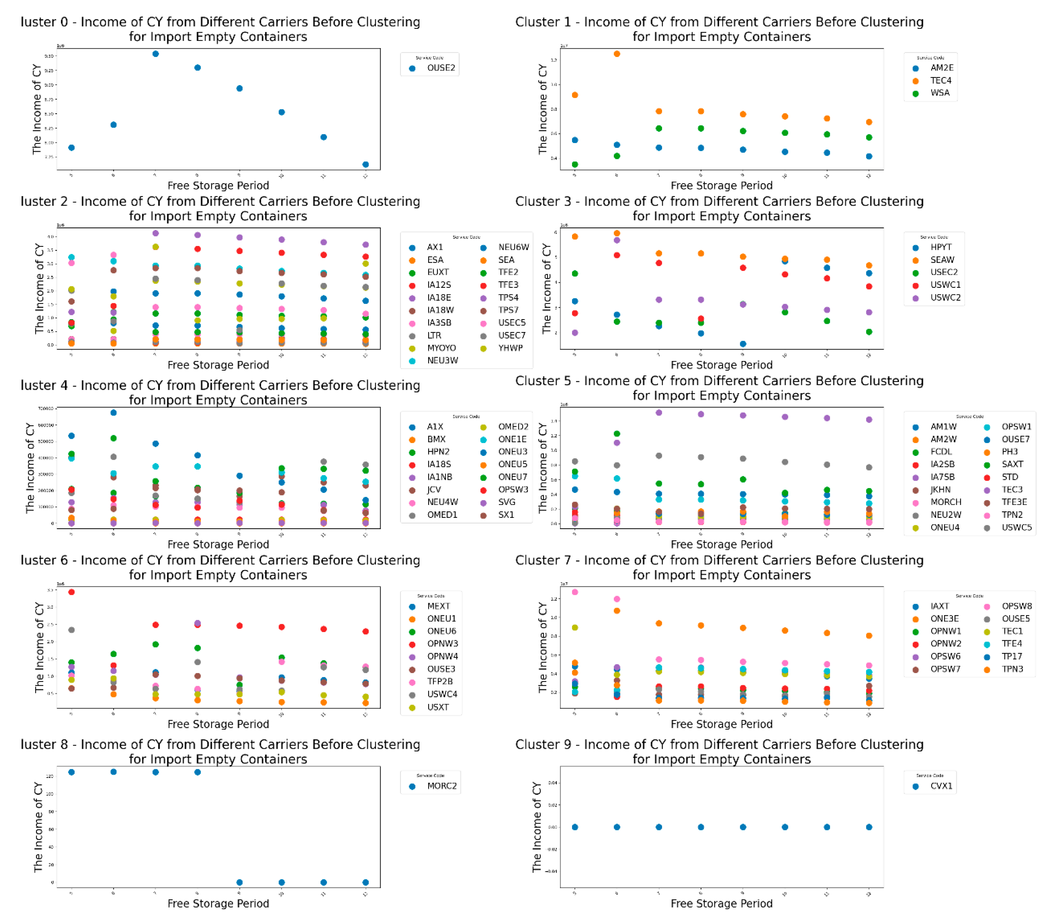
Figure 12.
The RCTY’s income under different free storage period for import empty containers before the clustering.
Figure 12.
The RCTY’s income under different free storage period for import empty containers before the clustering.
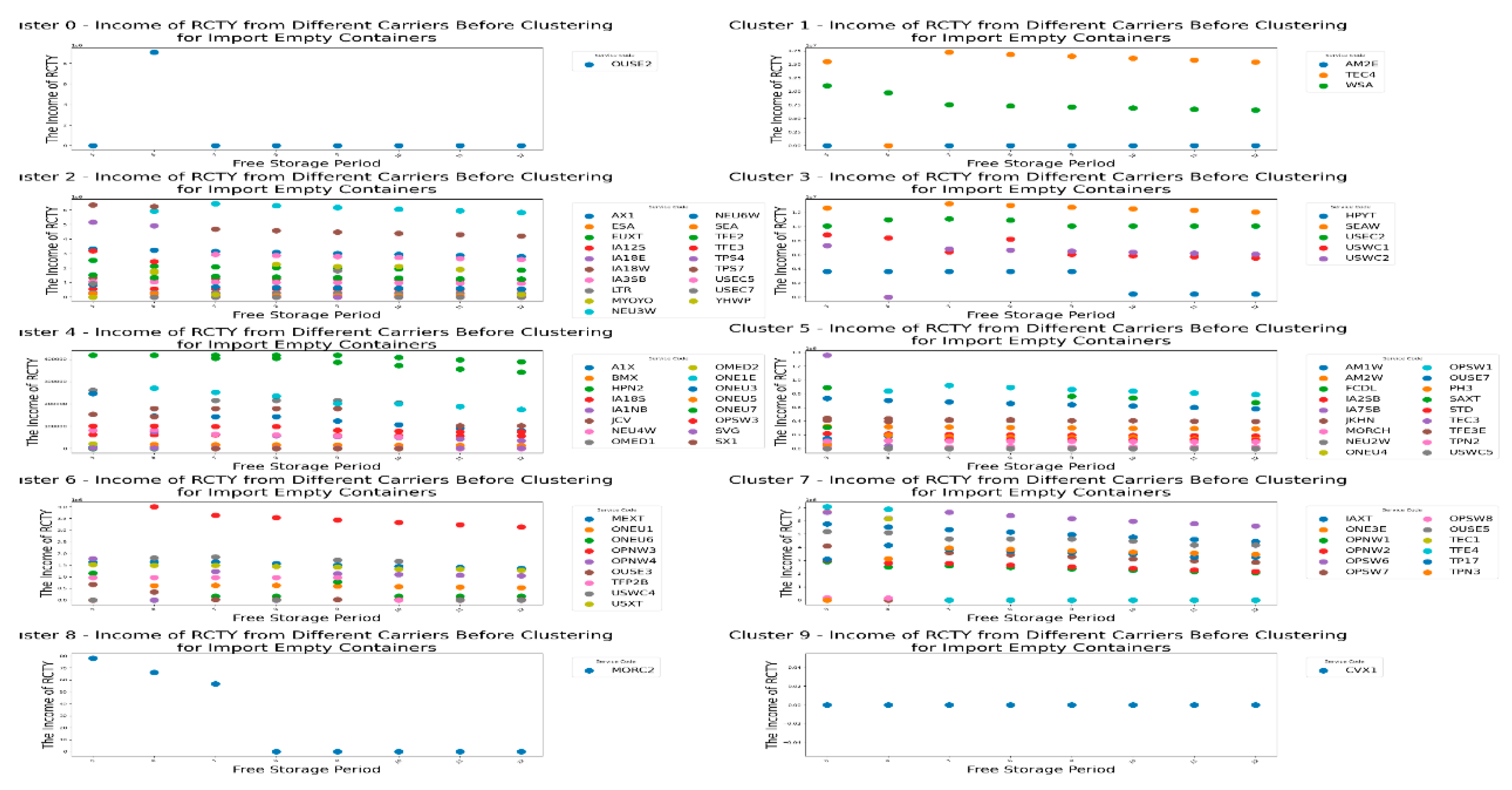
Figure 13.
The carrier’s cost under different free storage period for import empty containers before the clustering.
Figure 13.
The carrier’s cost under different free storage period for import empty containers before the clustering.
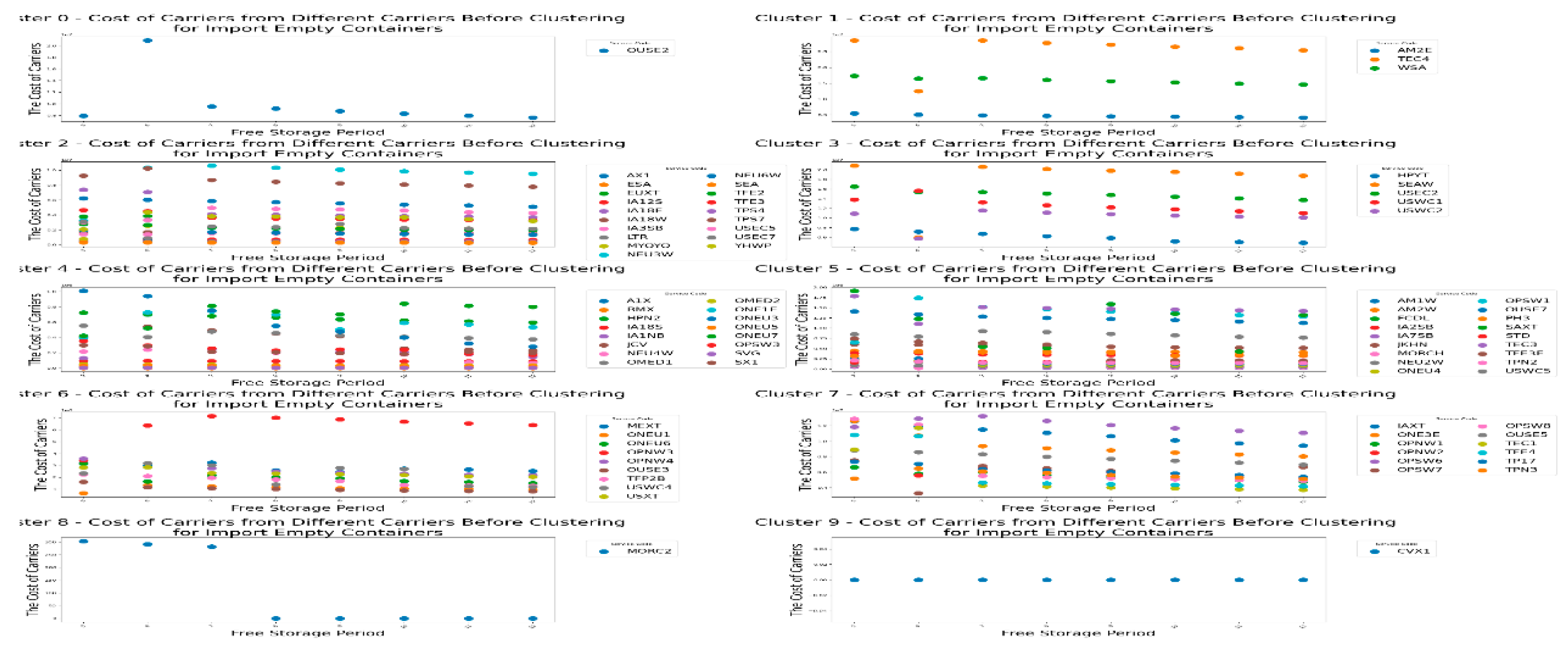
Figure 14.
The carrier’s transfer time under different free storage period for import empty containers before the clustering.
Figure 14.
The carrier’s transfer time under different free storage period for import empty containers before the clustering.
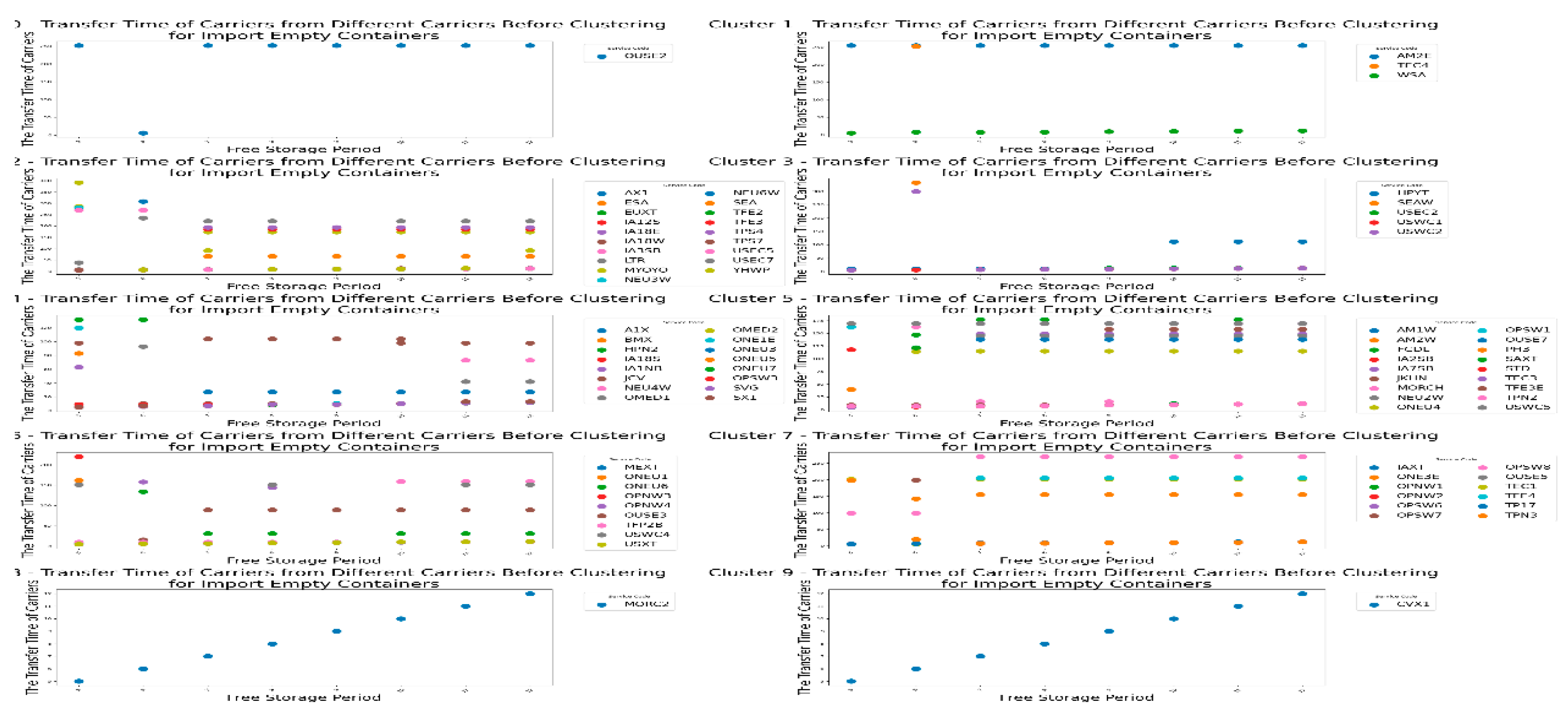
Figure 15.
The CY’s income under different pricing strategy range for import shipping containers before the clustering.
Figure 15.
The CY’s income under different pricing strategy range for import shipping containers before the clustering.
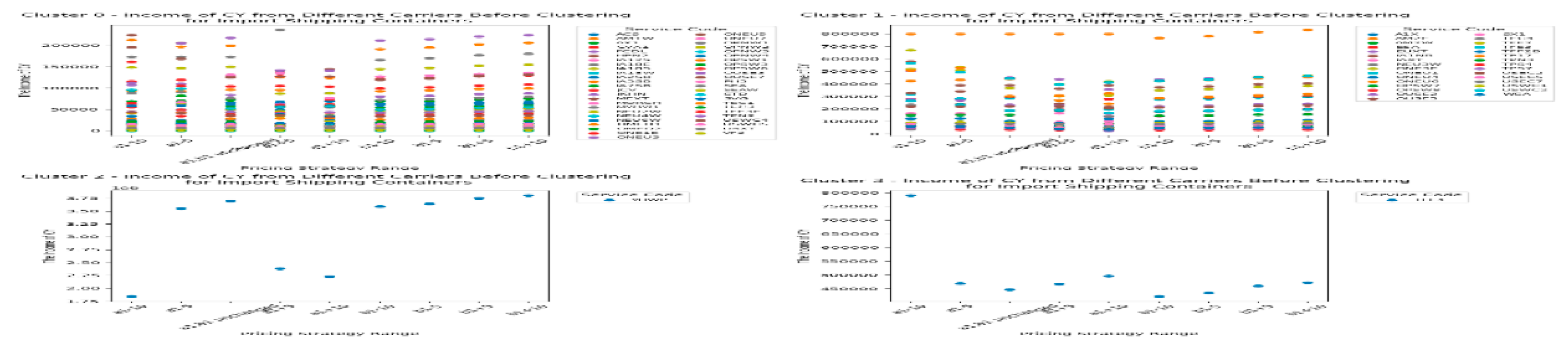
Figure 16.
The RCTY’s income under different pricing strategy range for import shipping containers before the clustering.
Figure 16.
The RCTY’s income under different pricing strategy range for import shipping containers before the clustering.
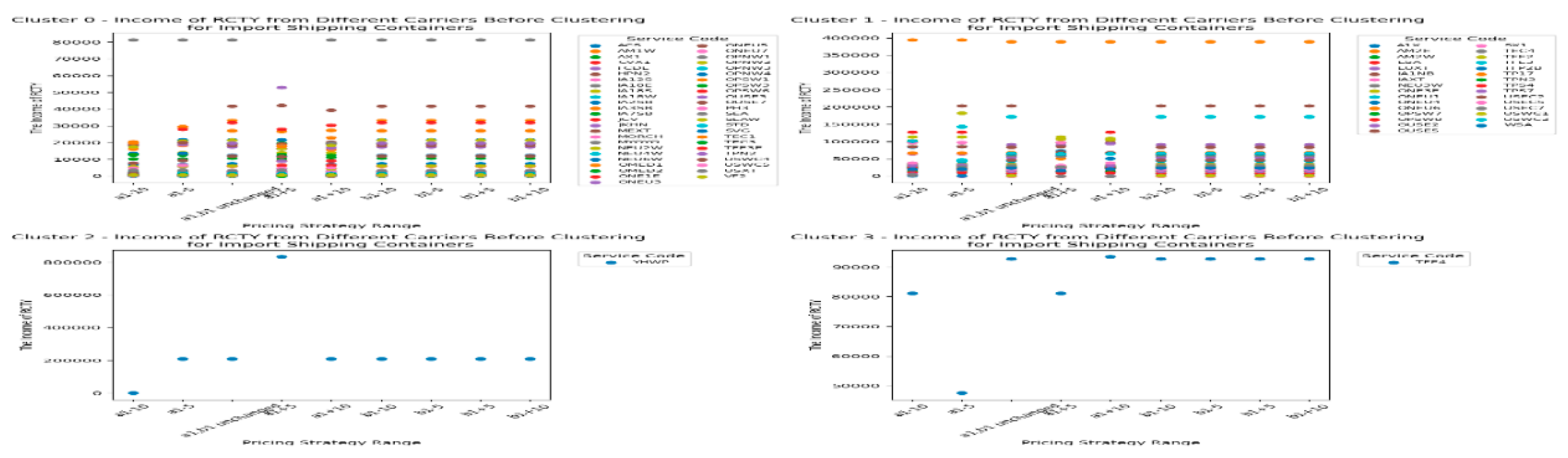
Figure 17.
The carrier’s cost under different pricing strategy range for import shipping containers before the clustering.
Figure 17.
The carrier’s cost under different pricing strategy range for import shipping containers before the clustering.
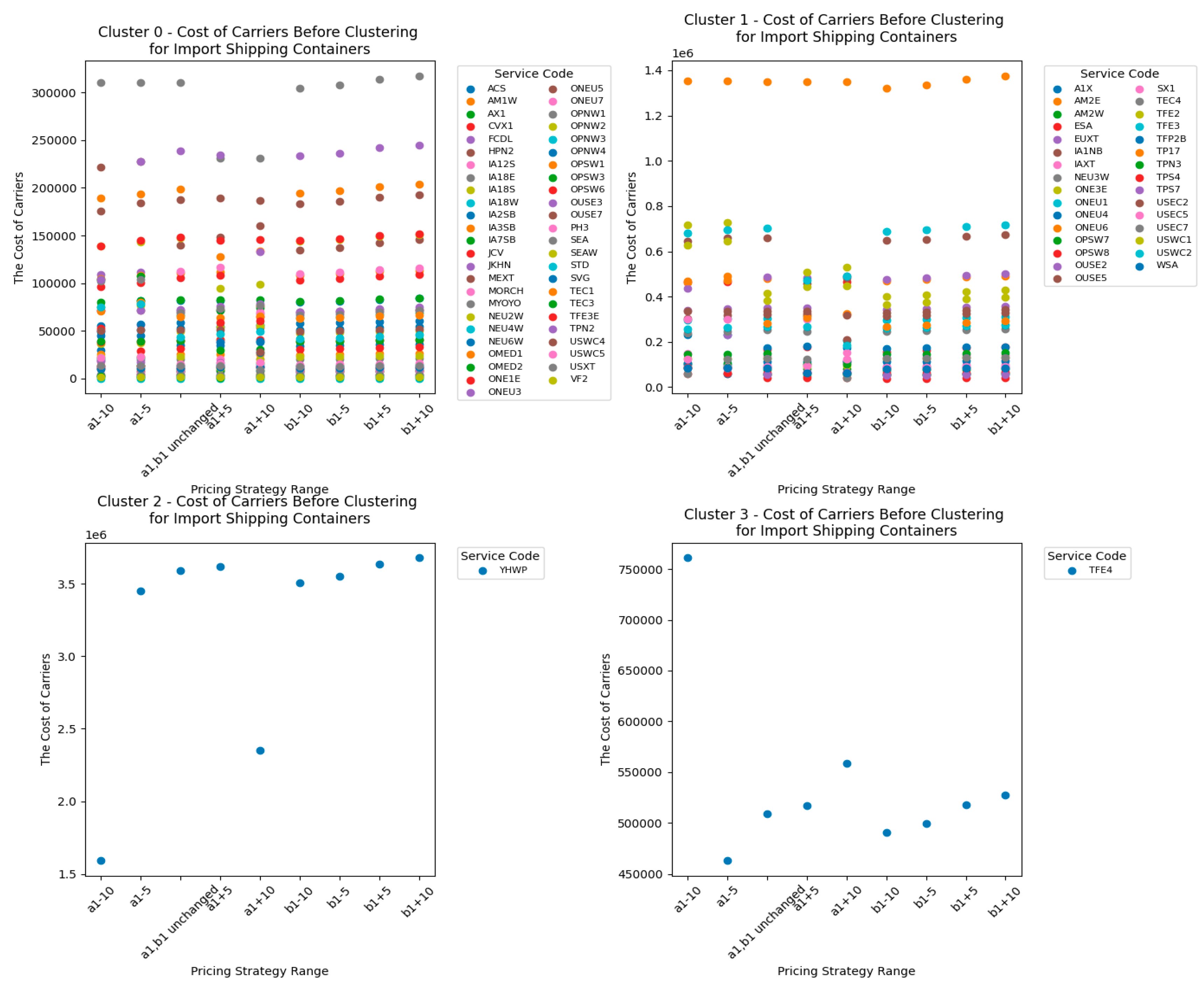
Figure 18.
The carrier’s transfer time under different pricing strategy range for import shipping containers before the clustering.
Figure 18.
The carrier’s transfer time under different pricing strategy range for import shipping containers before the clustering.
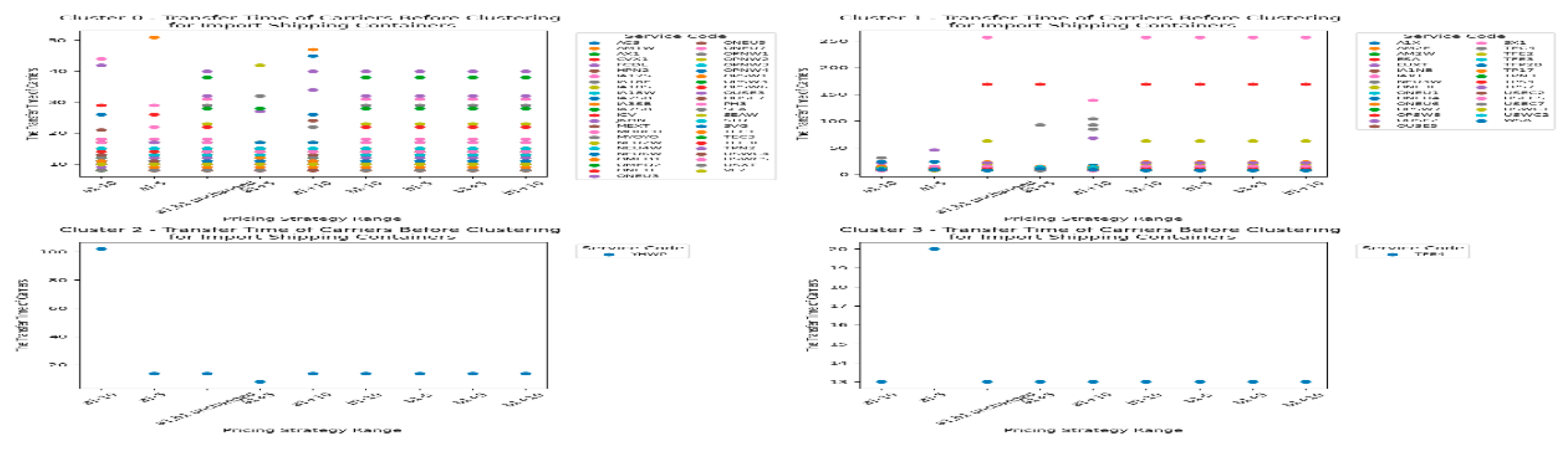
Figure 19.
The CY’s income under different free storage period for import shipping containers before the clustering.
Figure 19.
The CY’s income under different free storage period for import shipping containers before the clustering.
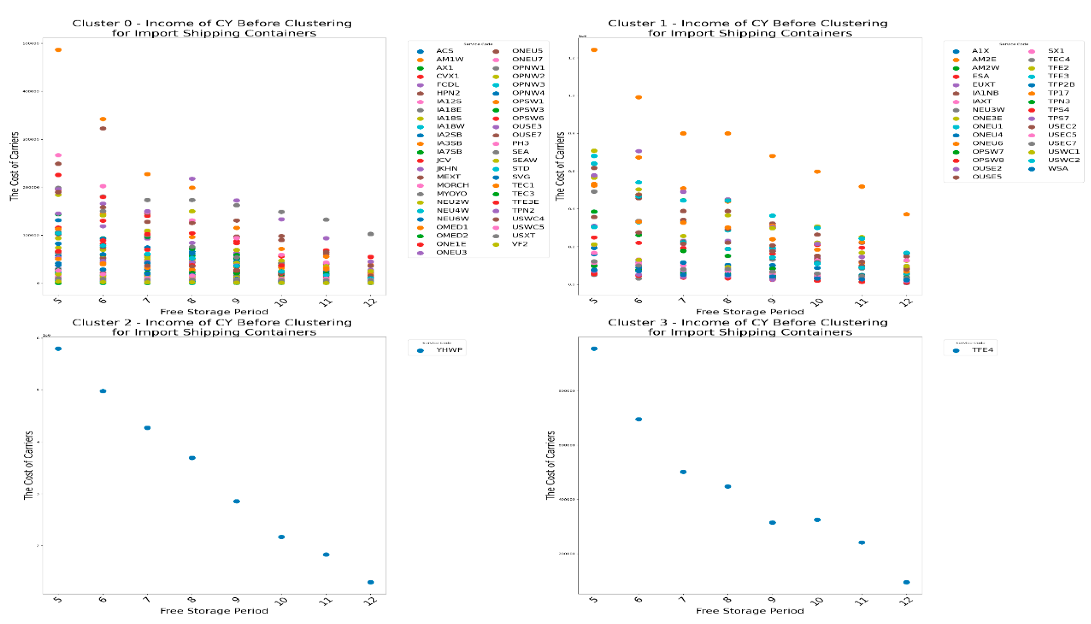
Figure 20.
The RCTY’s income under different free storage period for import shipping containers before the clustering.
Figure 20.
The RCTY’s income under different free storage period for import shipping containers before the clustering.
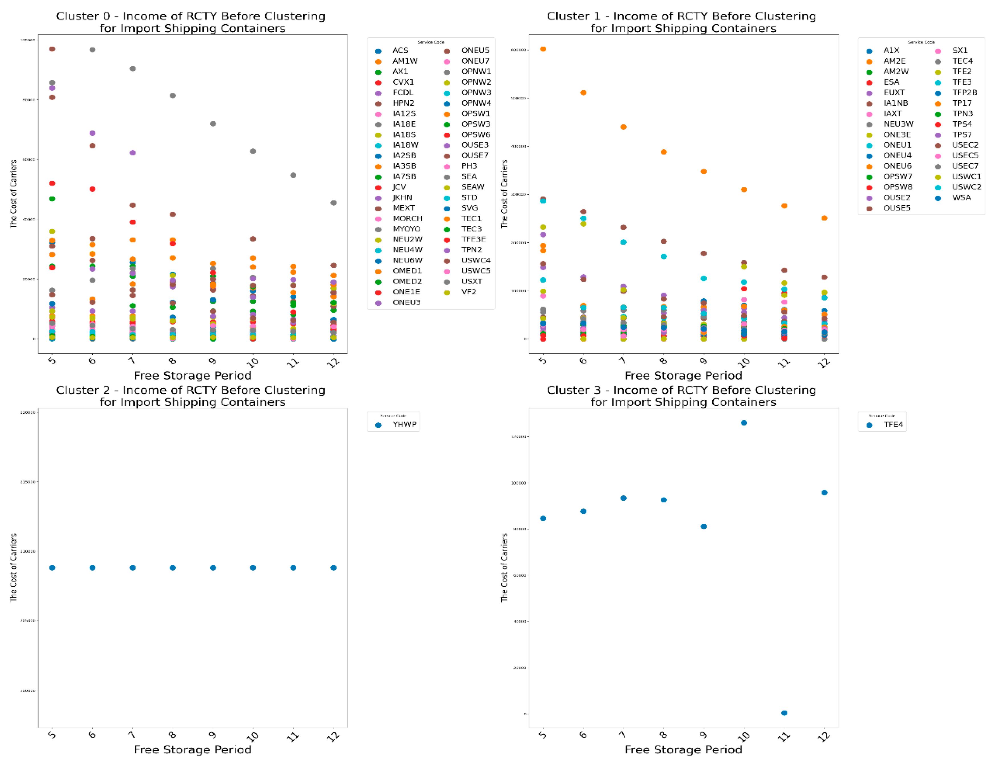
Figure 21.
The carrier’s cost under different free storage period for import shipping containers before the clustering.
Figure 21.
The carrier’s cost under different free storage period for import shipping containers before the clustering.
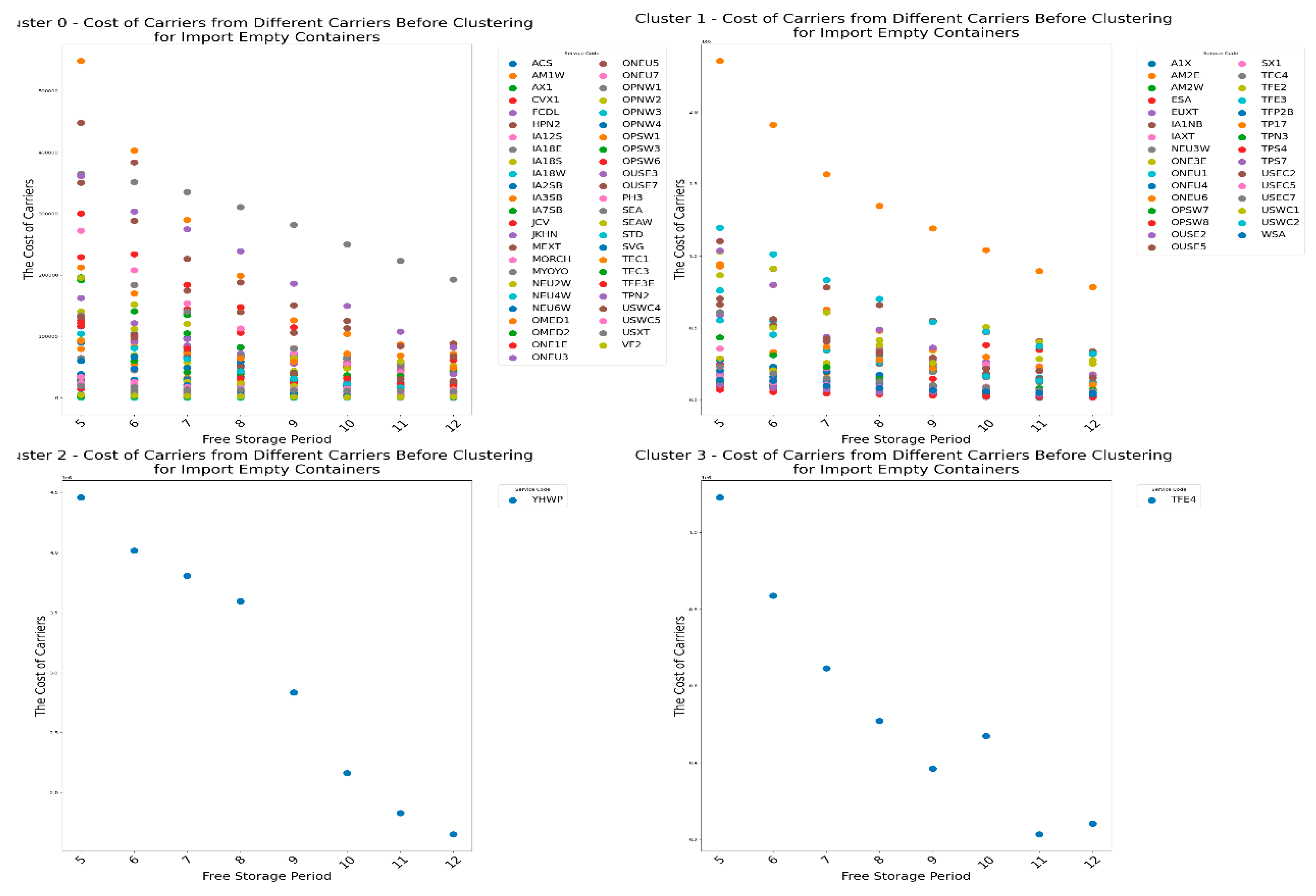
Figure 22.
The carrier’s transfer time under different free storage period for import shipping containers before the clustering.
Figure 22.
The carrier’s transfer time under different free storage period for import shipping containers before the clustering.
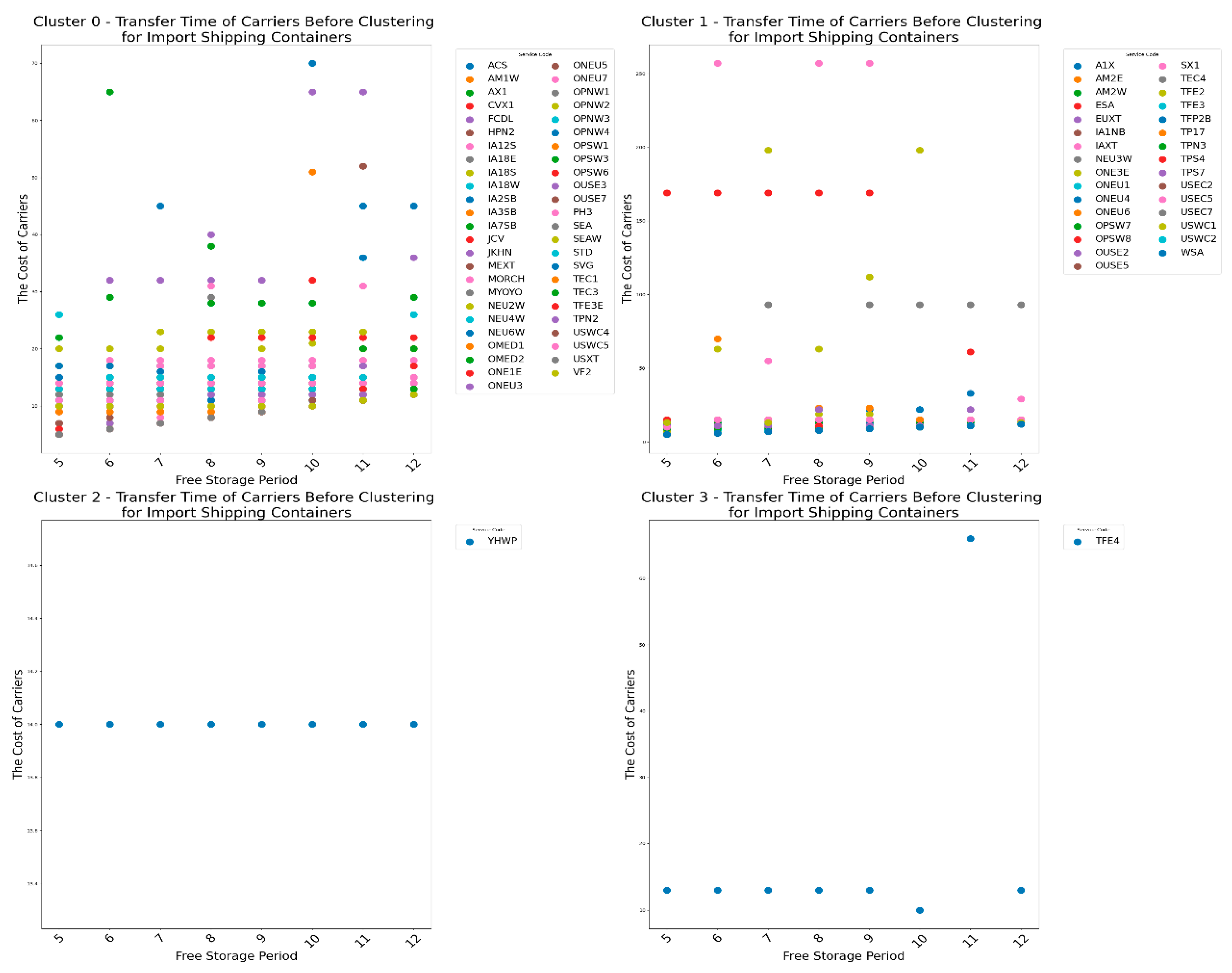
Figure 27.
The CY’s income under different free storage period for import empty containers after the clustering.
Figure 27.
The CY’s income under different free storage period for import empty containers after the clustering.
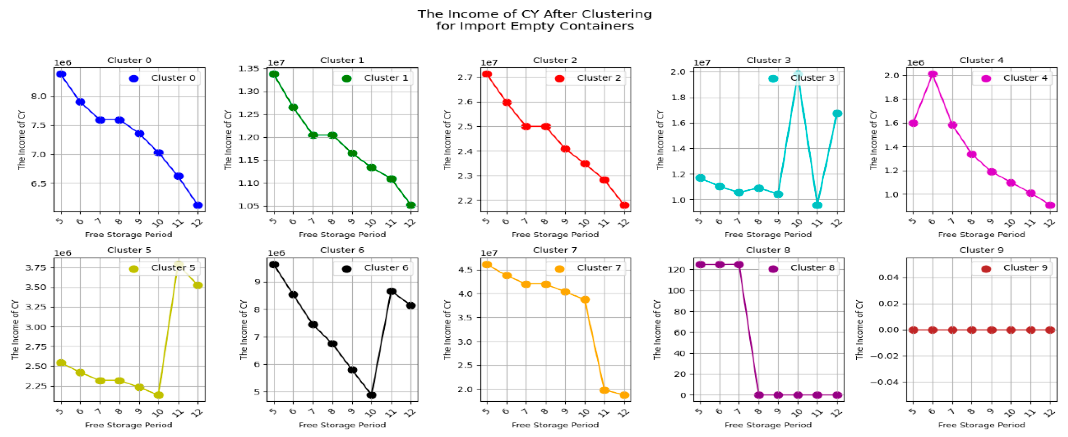
Figure 28.
The RCTY’s income under different free storage period for import empty containers after the clustering.
Figure 28.
The RCTY’s income under different free storage period for import empty containers after the clustering.
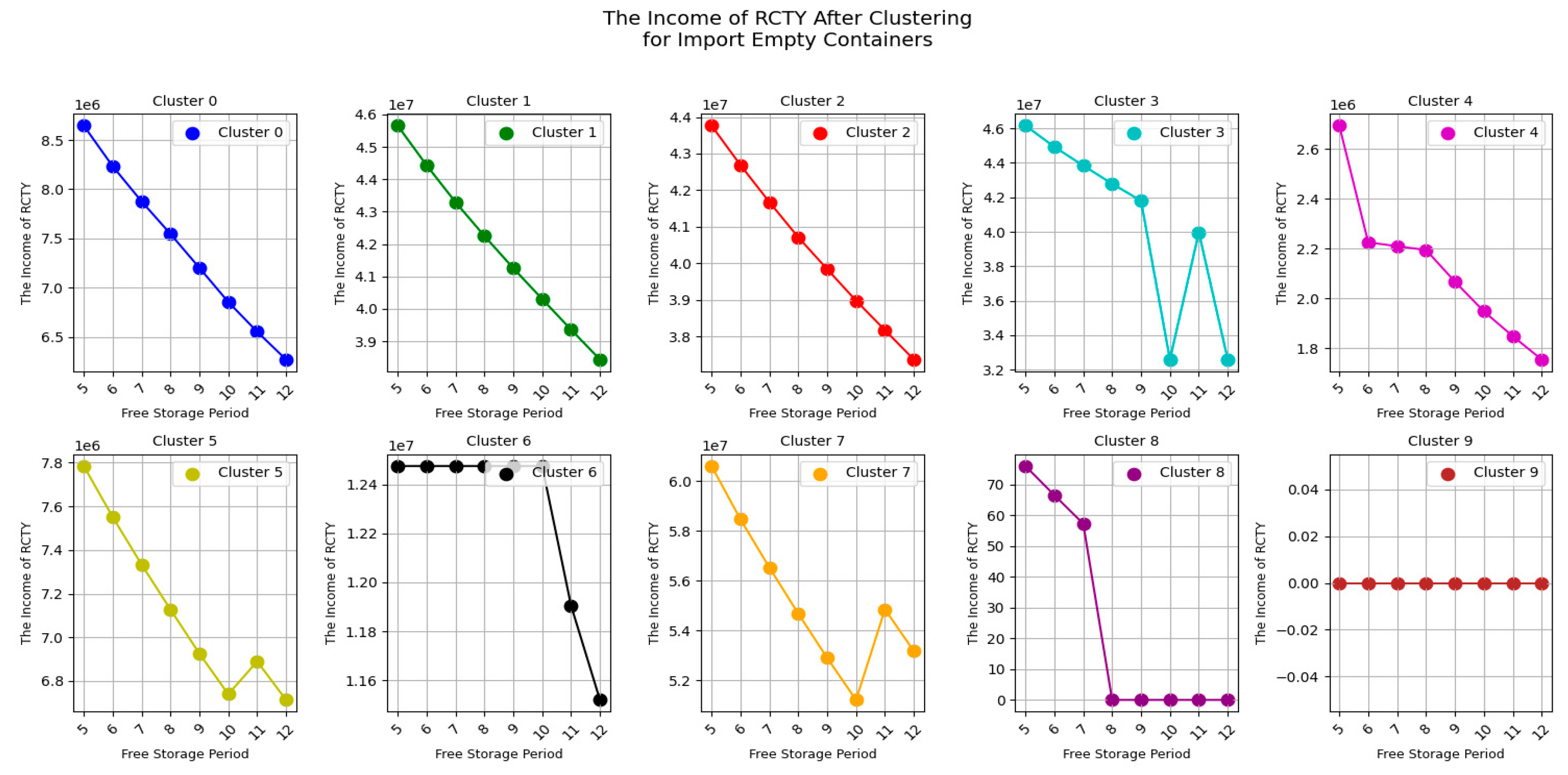
Figure 29.
The carrier’s cost under different free storage period for import empty containers after the clustering.
Figure 29.
The carrier’s cost under different free storage period for import empty containers after the clustering.
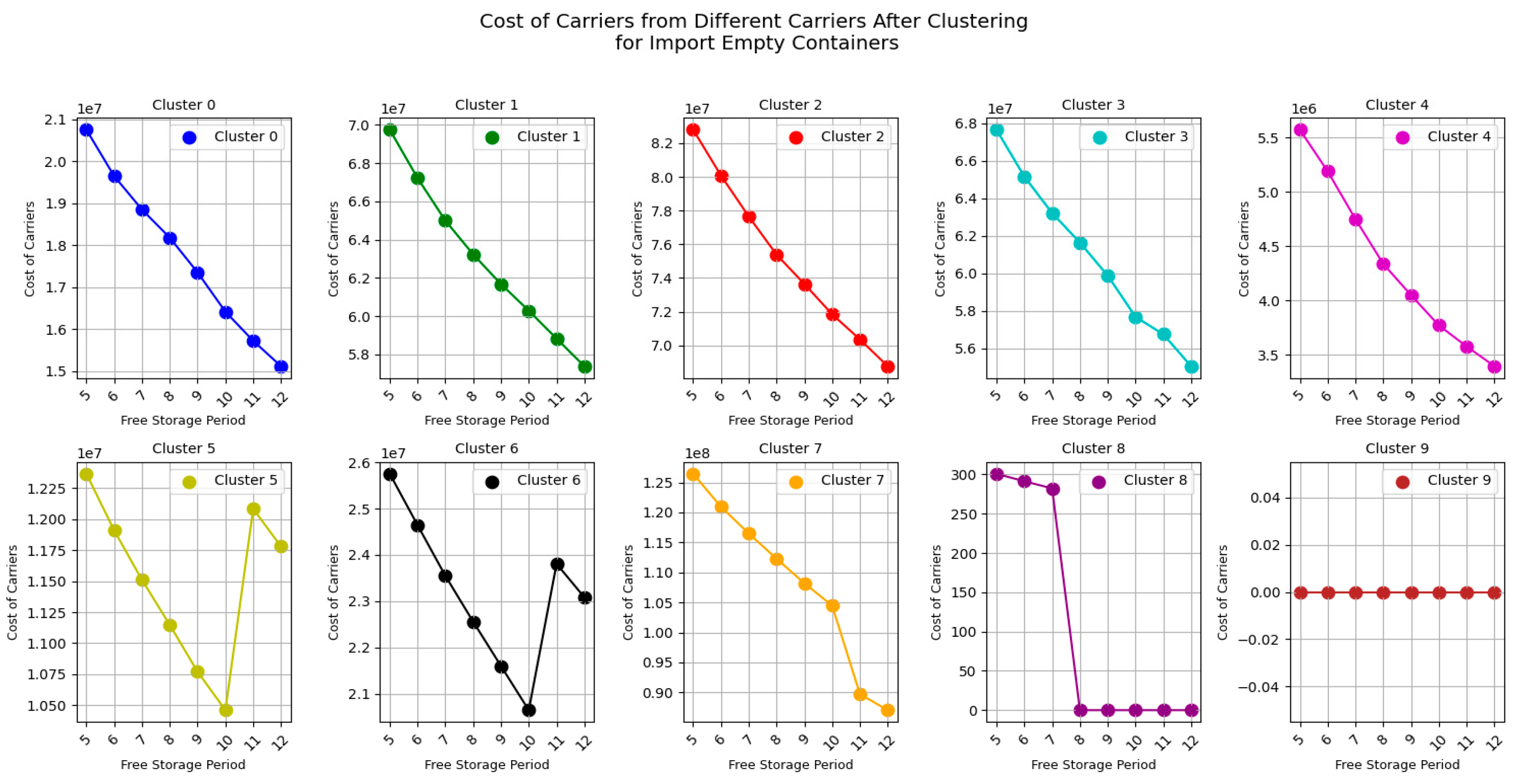
Figure 30.
The carrier’s transfer time under different free storage period for import empty containers after the clustering.
Figure 30.
The carrier’s transfer time under different free storage period for import empty containers after the clustering.
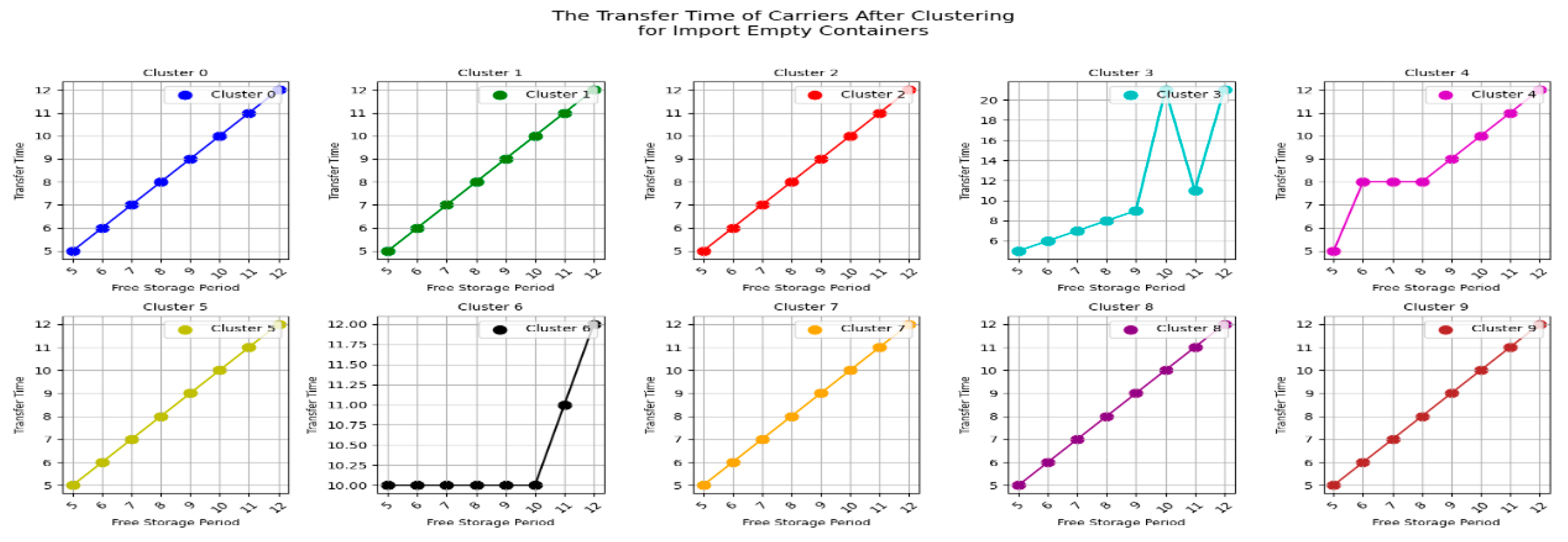
Figure 31.
The CY’s income under different pricing strategy scope for import shipping containers after the clustering.
Figure 31.
The CY’s income under different pricing strategy scope for import shipping containers after the clustering.
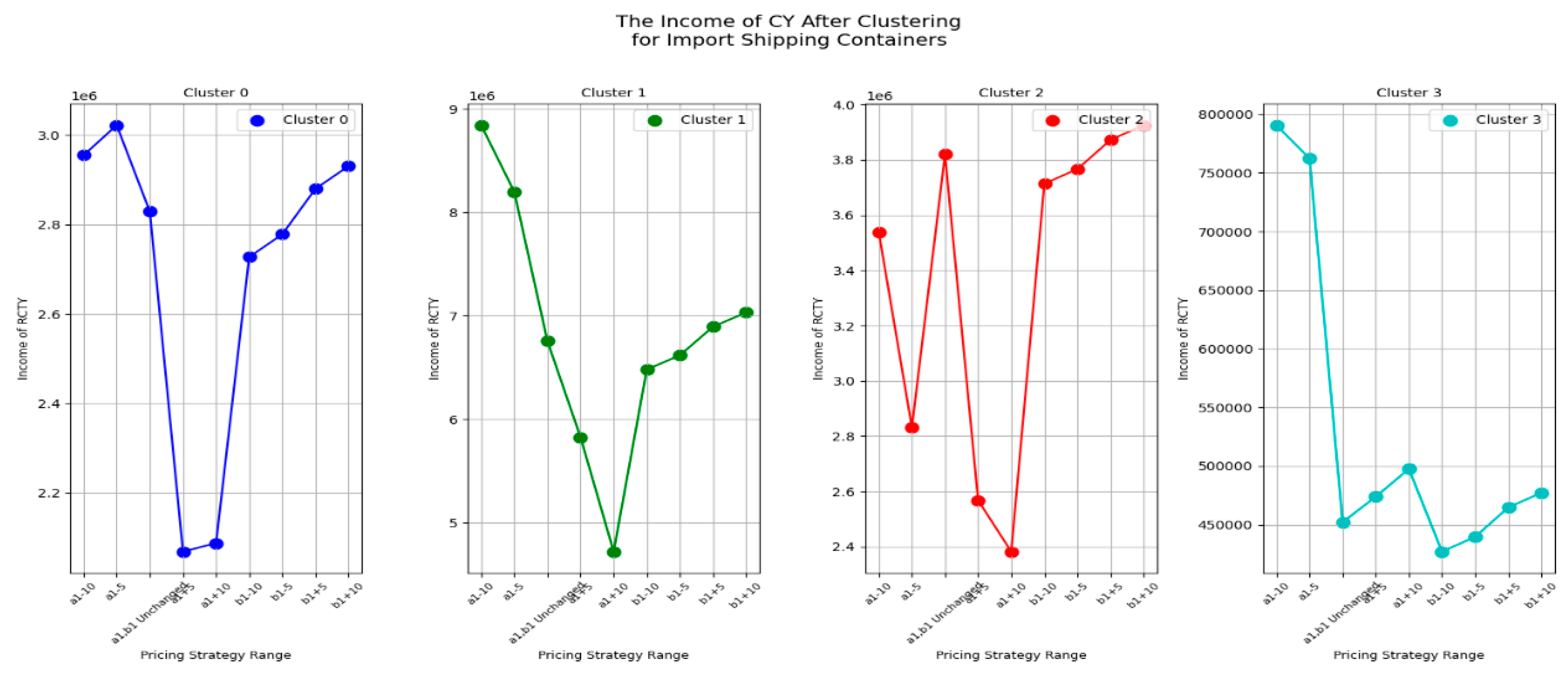
Figure 32.
The RCTY’s income under different pricing strategy scope for import shipping containers after the clustering.
Figure 32.
The RCTY’s income under different pricing strategy scope for import shipping containers after the clustering.
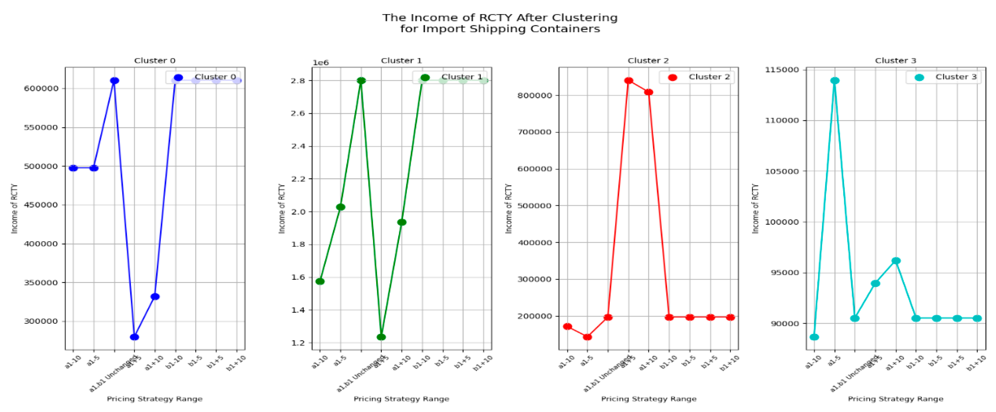
Figure 33.
The carrier’s cost under different pricing strategy scope for import shipping containers after the clustering.
Figure 33.
The carrier’s cost under different pricing strategy scope for import shipping containers after the clustering.
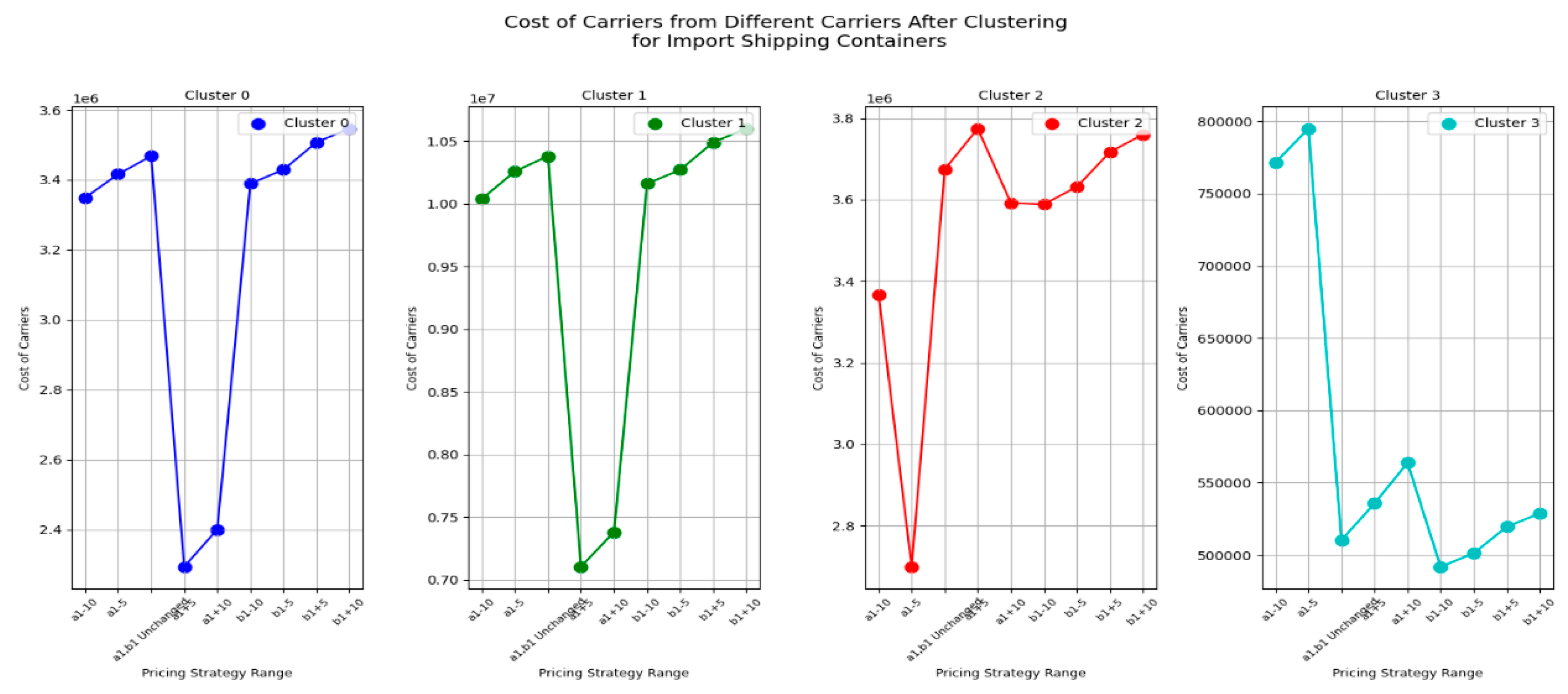
Figure 34.
The carrier’s transfer time under different pricing strategy scope for import shipping containers after the clustering.
Figure 34.
The carrier’s transfer time under different pricing strategy scope for import shipping containers after the clustering.
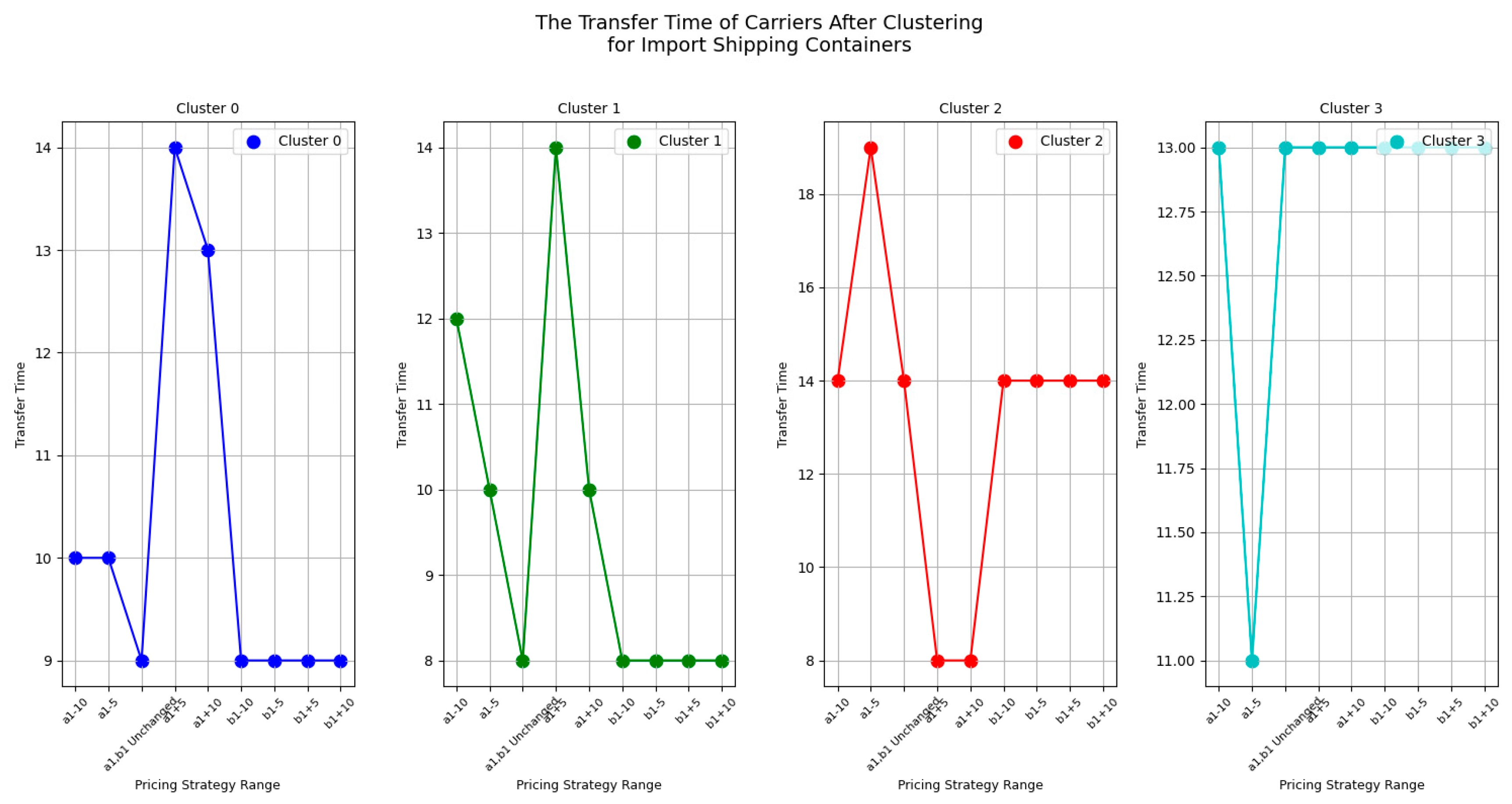
Figure 35.
The CY’s income under different free storage period for import shipping containers after the clustering.
Figure 35.
The CY’s income under different free storage period for import shipping containers after the clustering.
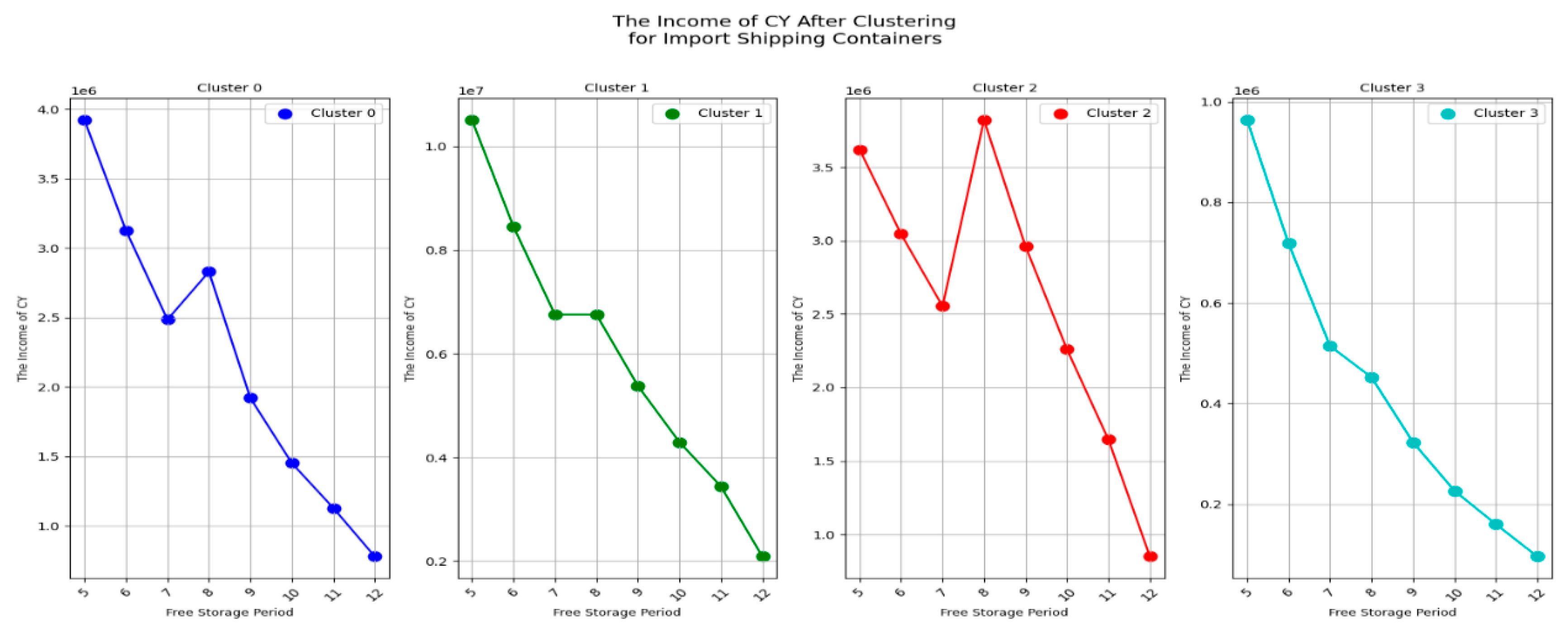
Figure 36.
The mean and median of the RCTY’s income under different free storage period for import shipping containers after the clustering.
Figure 36.
The mean and median of the RCTY’s income under different free storage period for import shipping containers after the clustering.
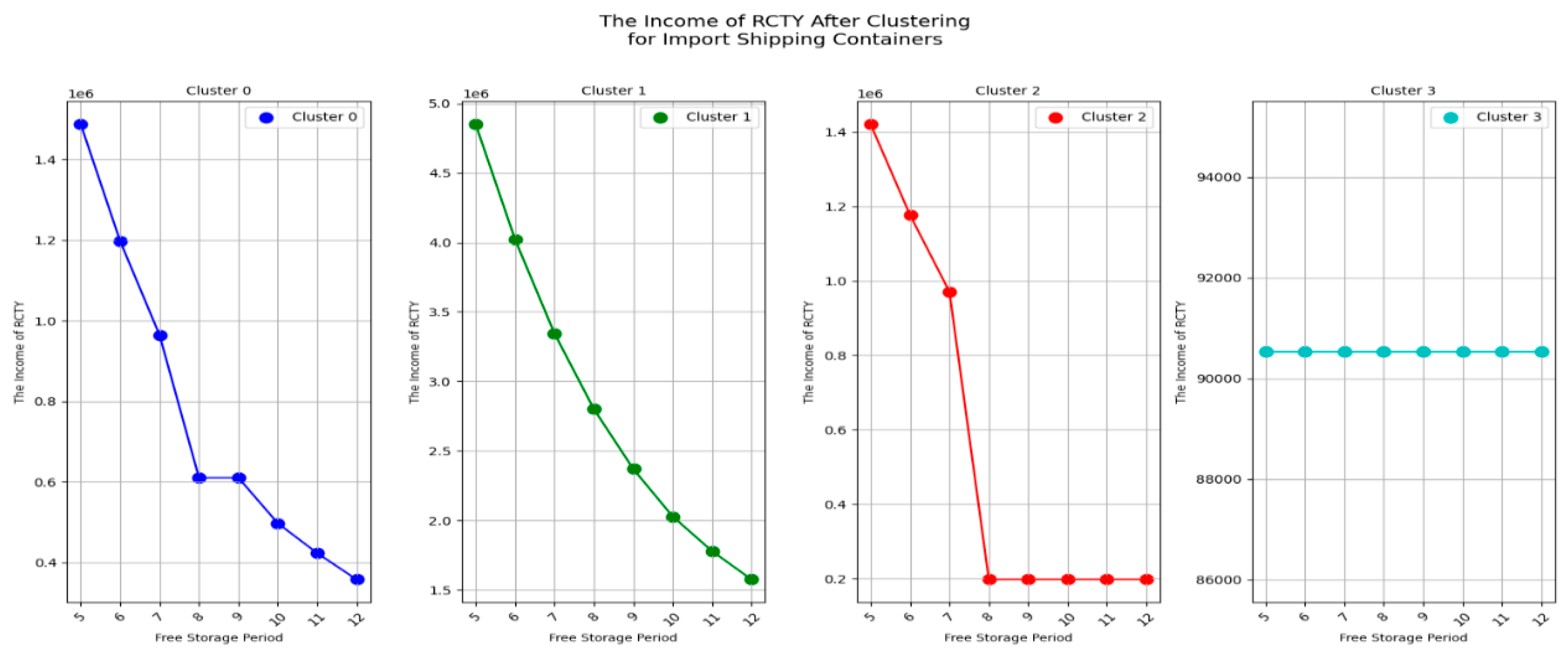
Figure 37.
The carrier’s cost under different free storage period for import shipping containers after the clustering.
Figure 37.
The carrier’s cost under different free storage period for import shipping containers after the clustering.
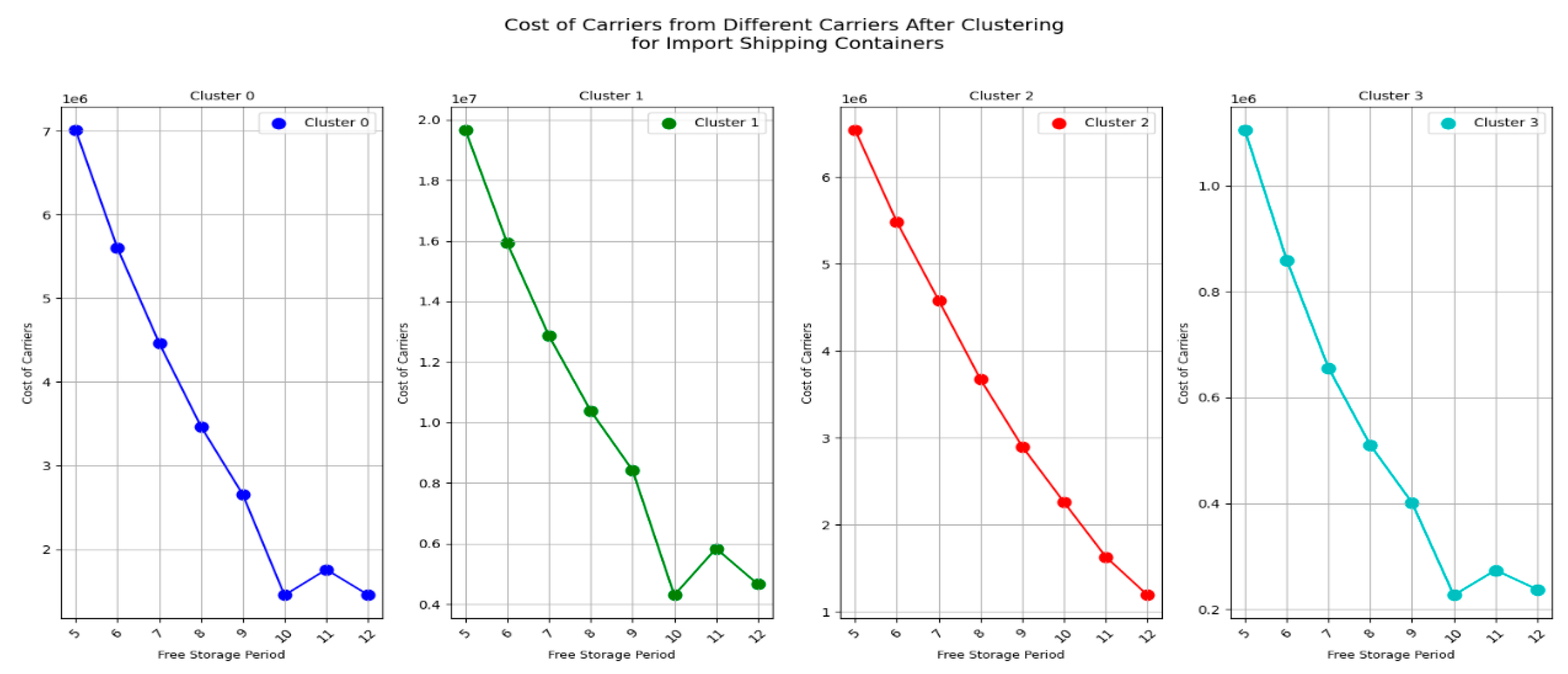
Figure 38.
The carrier’s transfer time under different free storage period for import shipping containers after the clustering.
Figure 38.
The carrier’s transfer time under different free storage period for import shipping containers after the clustering.
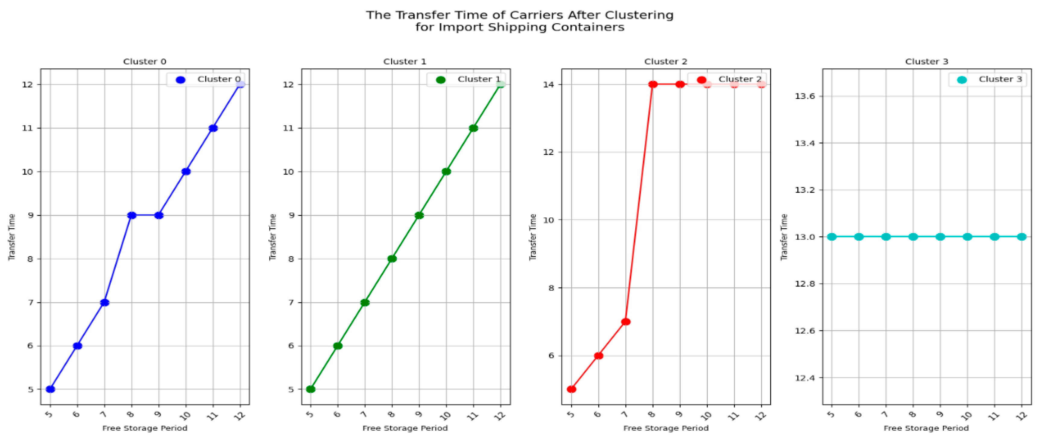
Figure 39.
CY’s Income for Different Pricing Strategy Rages, Showing the Values Across Each Cluster Before and After Clustering of Import Empty Containers.
Figure 39.
CY’s Income for Different Pricing Strategy Rages, Showing the Values Across Each Cluster Before and After Clustering of Import Empty Containers.
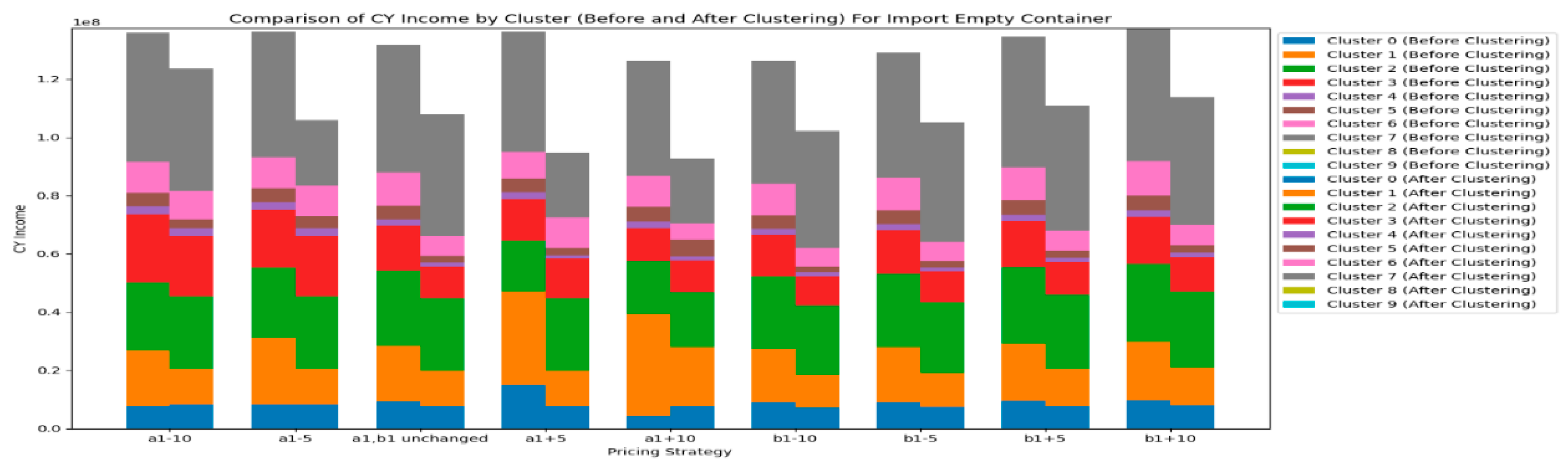
Figure 40.
RCTY’s Income for Different Pricing Strategy Rages, Showing the Values Across Each Cluster Before and After Clustering of Import Empty Containers.
Figure 40.
RCTY’s Income for Different Pricing Strategy Rages, Showing the Values Across Each Cluster Before and After Clustering of Import Empty Containers.
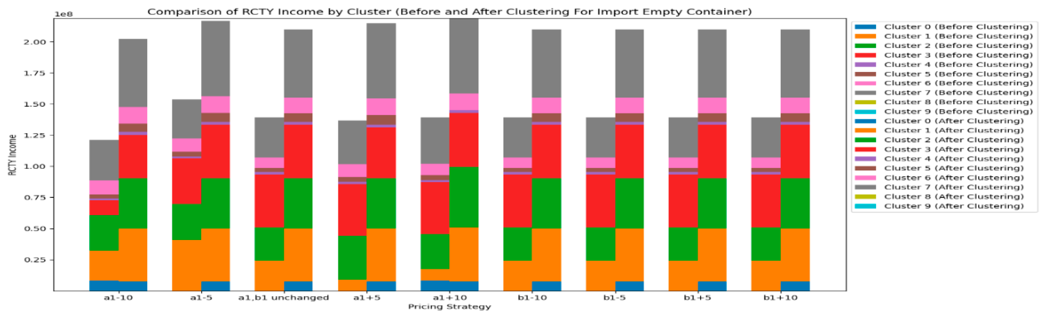
Figure 41.
Carrier’s Cost for Different Pricing Strategy Rages, Showing the Values Across Each Cluster Before and After Clustering of Import Empty Containers.
Figure 41.
Carrier’s Cost for Different Pricing Strategy Rages, Showing the Values Across Each Cluster Before and After Clustering of Import Empty Containers.
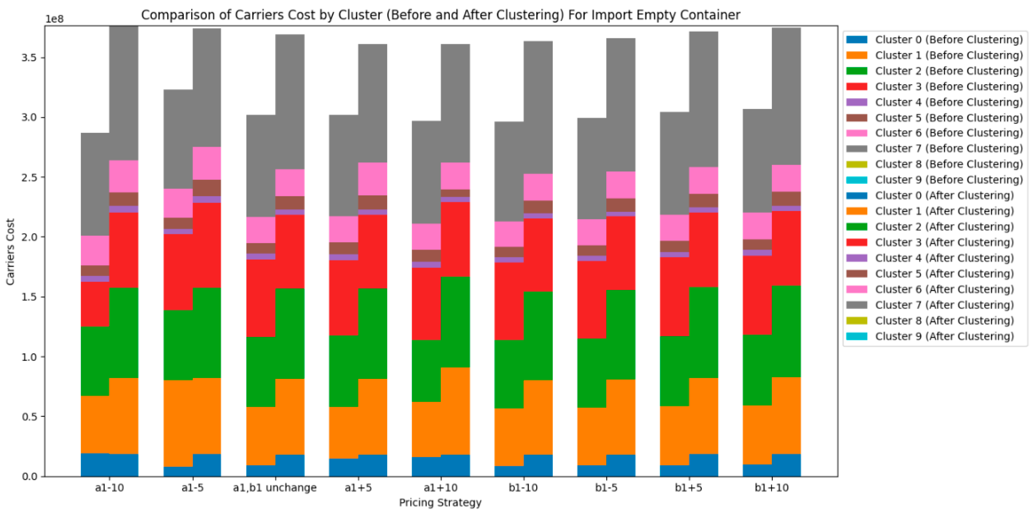
Figure 42.
CY’s Income for Different Pricing Strategy Ranges, Showing the Values Across Each Cluster Before and After Clustering of Import Shipping Containers.
Figure 42.
CY’s Income for Different Pricing Strategy Ranges, Showing the Values Across Each Cluster Before and After Clustering of Import Shipping Containers.
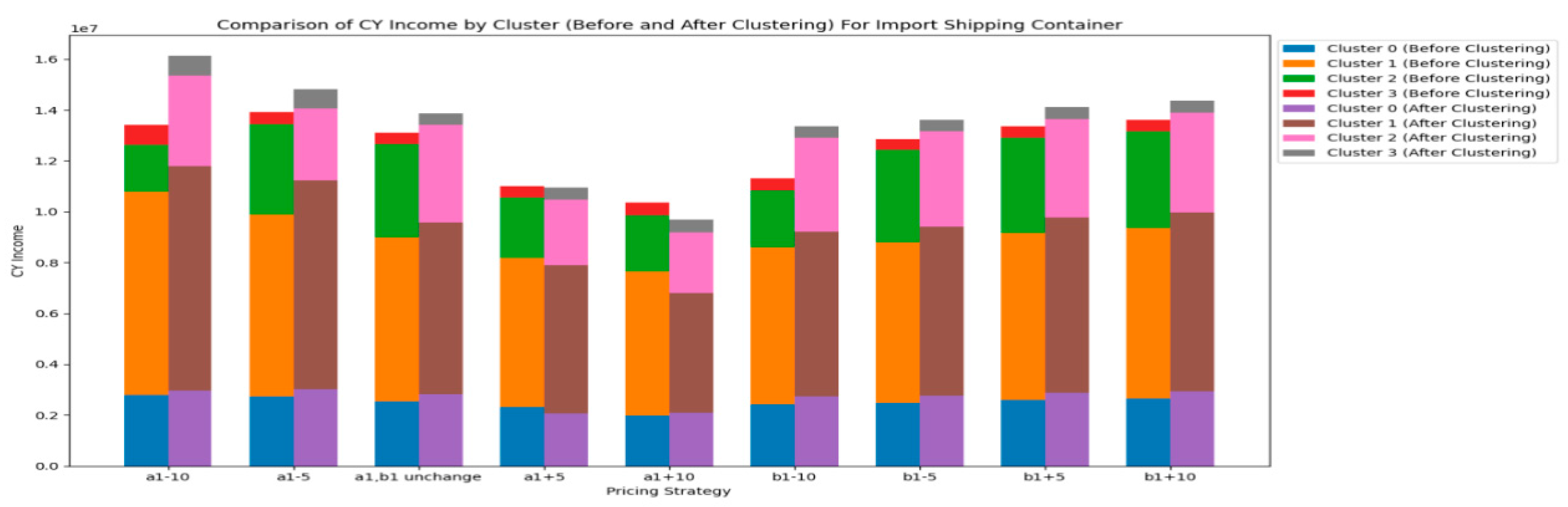
Figure 43.
RCTY’s Income for Different Pricing Strategy Ranges, Showing the Values Across Each Cluster Before and After Clustering of Import Shipping Containers.
Figure 43.
RCTY’s Income for Different Pricing Strategy Ranges, Showing the Values Across Each Cluster Before and After Clustering of Import Shipping Containers.
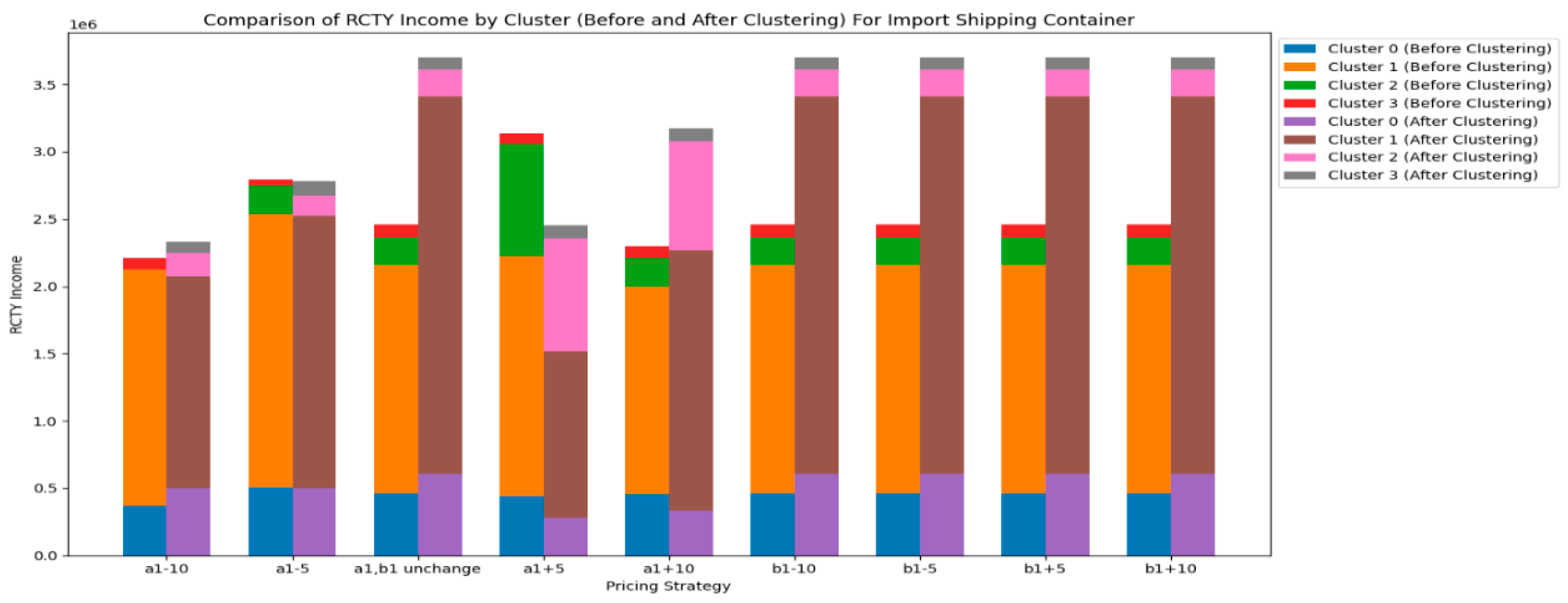
Figure 44.
Carrier’s Cost for Different Pricing Strategy Ranges, Showing the Values Across Each Cluster Before and After Clustering of Import Shipping Containers.
Figure 44.
Carrier’s Cost for Different Pricing Strategy Ranges, Showing the Values Across Each Cluster Before and After Clustering of Import Shipping Containers.
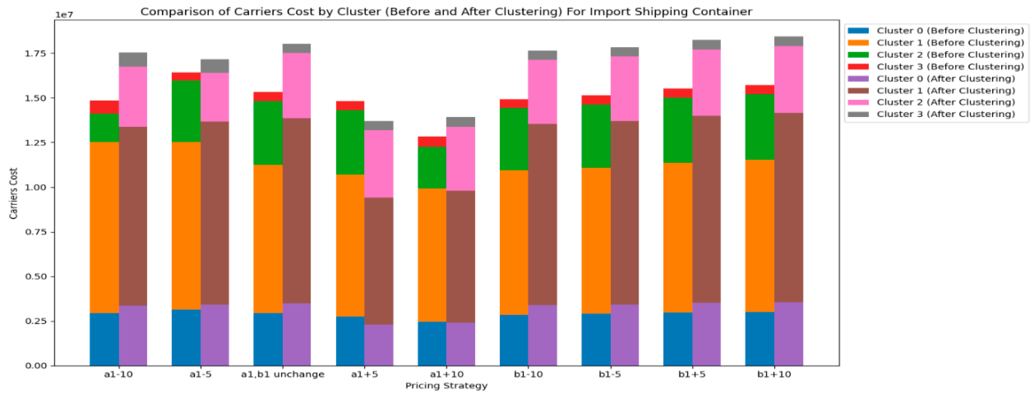
Figure 45.
CY’s Income for Different Free Storage Periods, Showing the Values Across Each Cluster Before and After Clustering of Import Empty Containers.
Figure 45.
CY’s Income for Different Free Storage Periods, Showing the Values Across Each Cluster Before and After Clustering of Import Empty Containers.
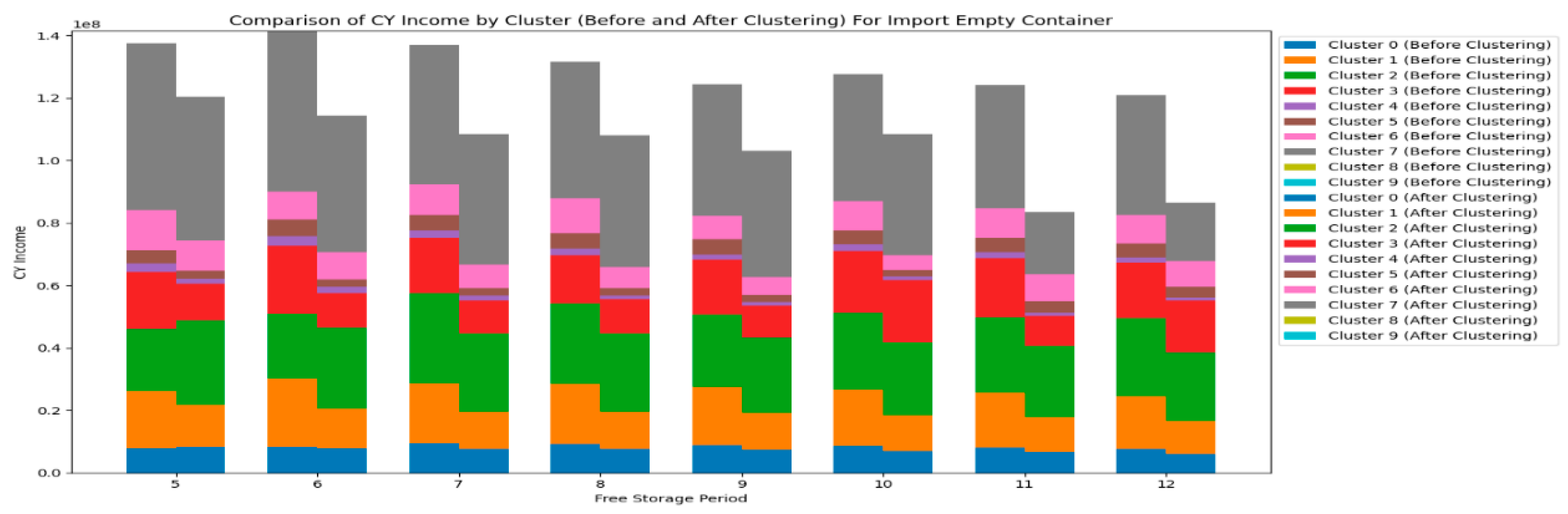
Figure 46.
RCTY’s Income for Different Free Storage Periods, Showing the Values Across Each Cluster Before and After Clustering of Import Empty Containers.
Figure 46.
RCTY’s Income for Different Free Storage Periods, Showing the Values Across Each Cluster Before and After Clustering of Import Empty Containers.
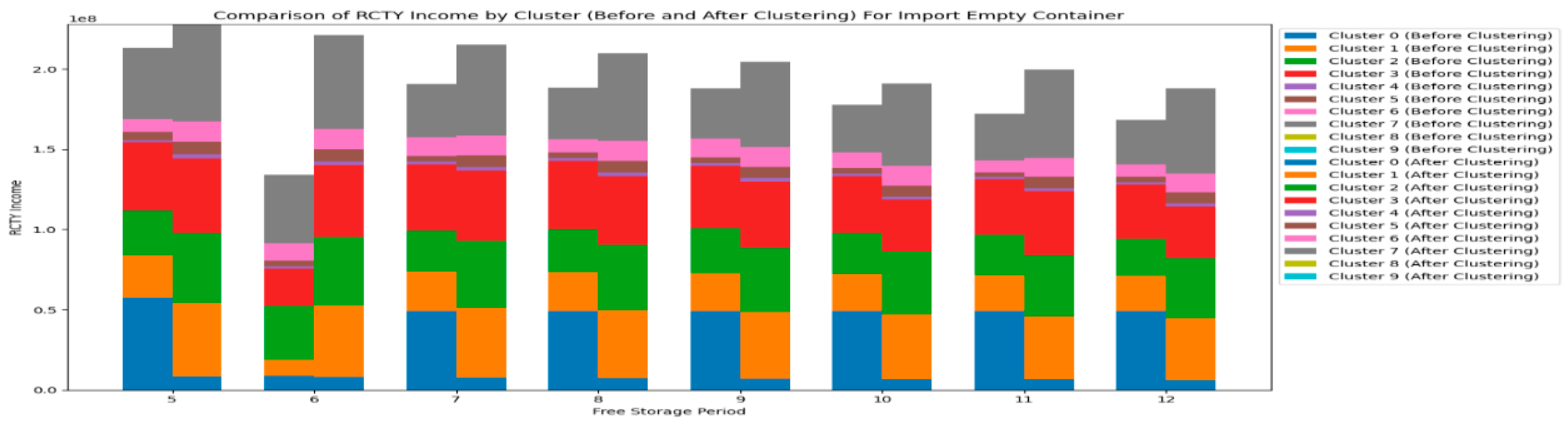
Figure 47.
Carrier’s Cost for Different Free Storage Periods, Showing the Values Across Each Cluster Before and After Clustering of Import Empty Containers.
Figure 47.
Carrier’s Cost for Different Free Storage Periods, Showing the Values Across Each Cluster Before and After Clustering of Import Empty Containers.
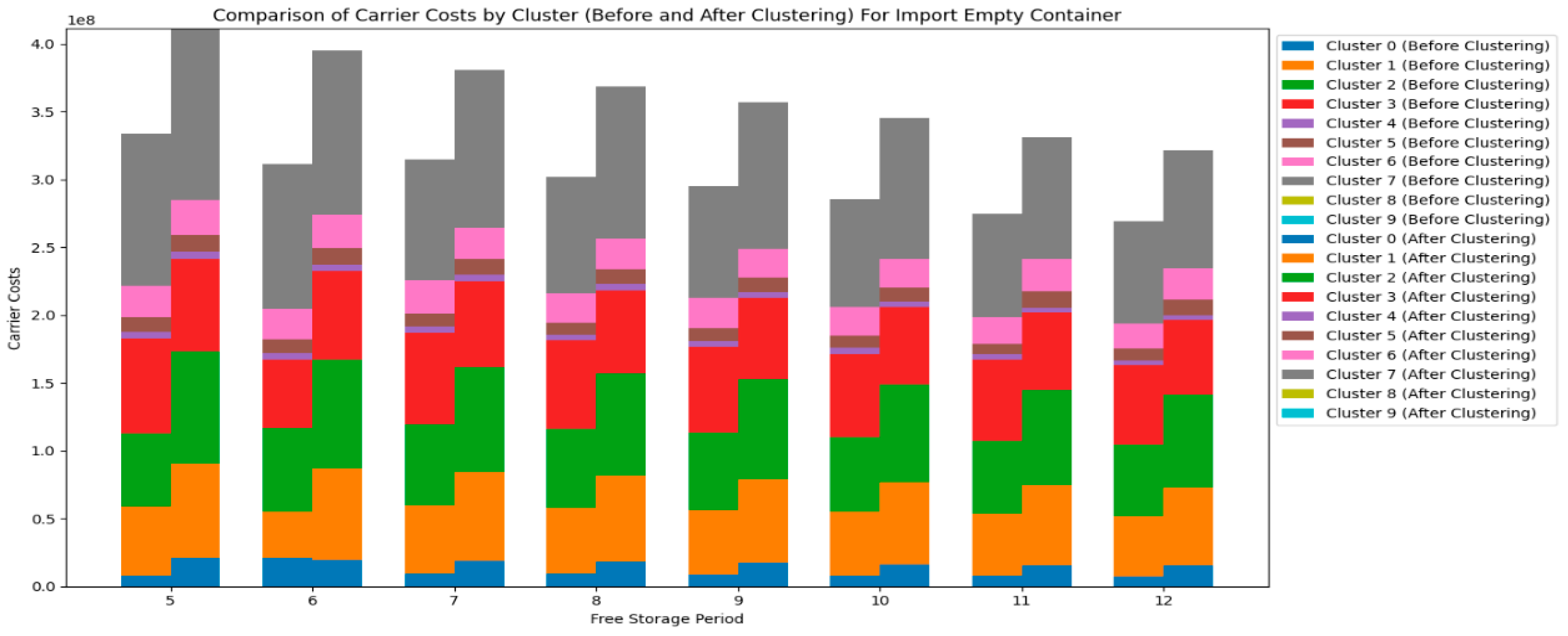
Figure 48.
CY’s Income for Different Free Storage Periods, Showing the Values Across Each Cluster Before and After Clustering of Import Shipping Containers.
Figure 48.
CY’s Income for Different Free Storage Periods, Showing the Values Across Each Cluster Before and After Clustering of Import Shipping Containers.
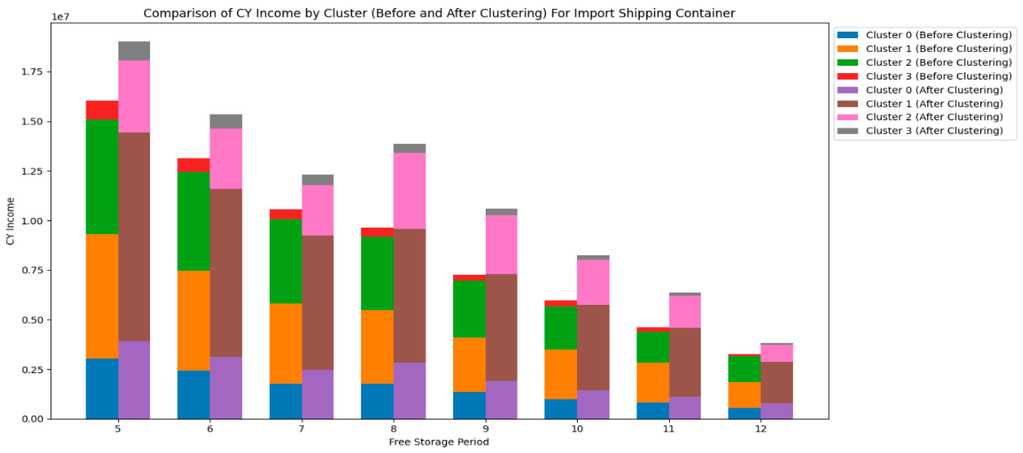
Figure 49.
RCTY’s Income for Different Free Storage Periods, Showing the Values Across Each Cluster Before and After Clustering of Import Shipping Containers.
Figure 49.
RCTY’s Income for Different Free Storage Periods, Showing the Values Across Each Cluster Before and After Clustering of Import Shipping Containers.
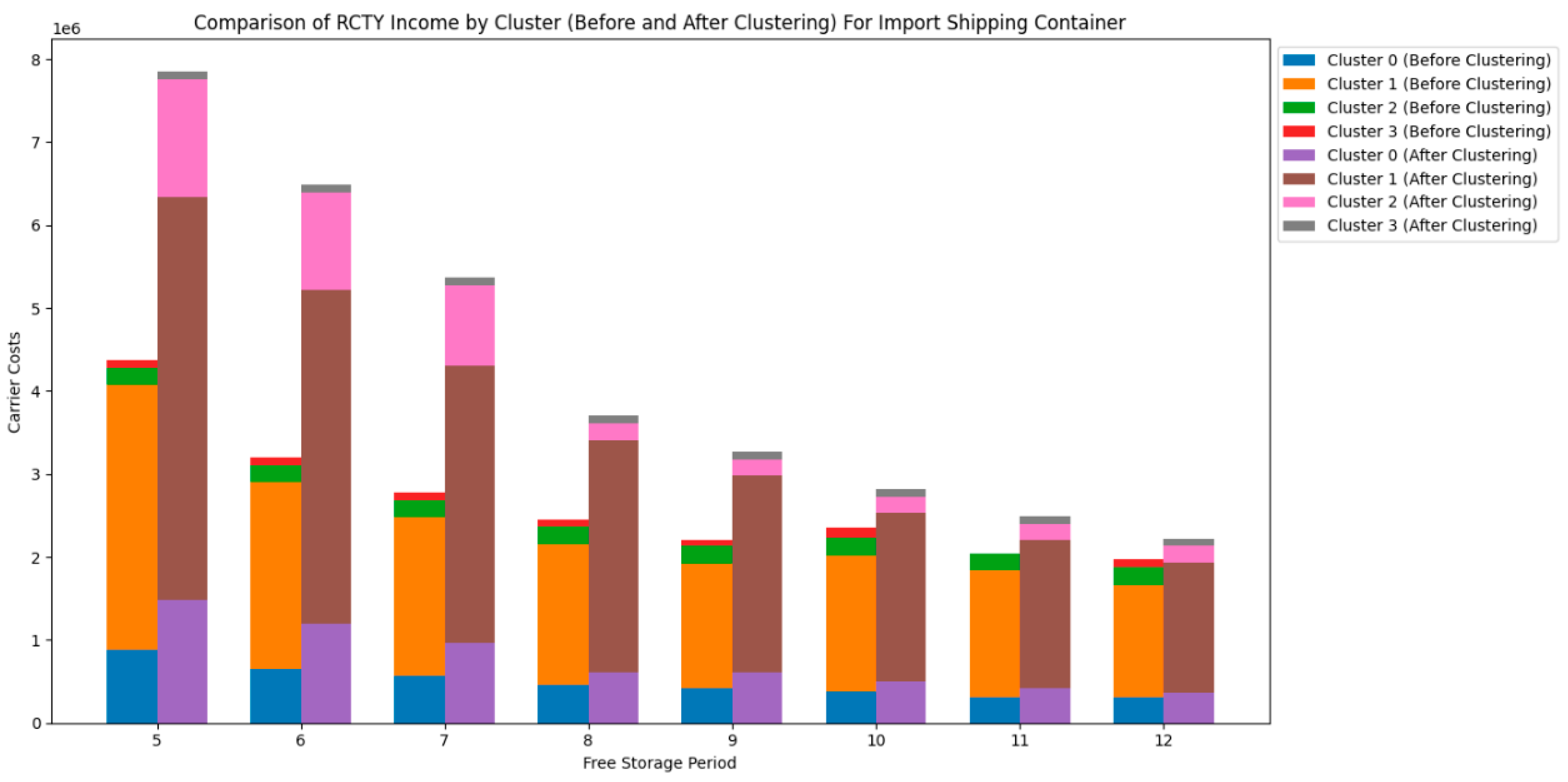
Figure 50.
Carrier’s Cost for Different Free Storage Periods, Showing the Values Across Each Cluster Before and After Clustering of Import Shipping Containers.
Figure 50.
Carrier’s Cost for Different Free Storage Periods, Showing the Values Across Each Cluster Before and After Clustering of Import Shipping Containers.
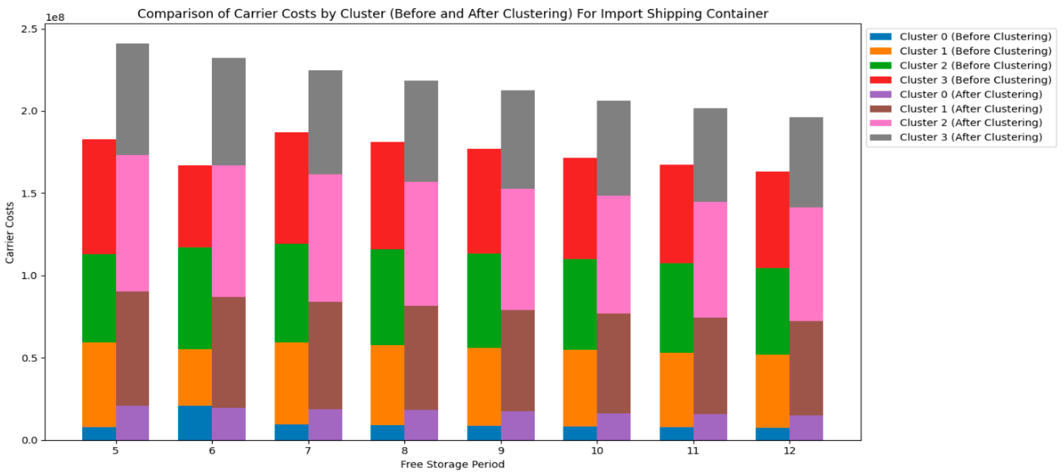
Table 1.
Feature extraction during data clustering.
| Clustering Algorithms | Selecting Features |
|---|---|
| K-means Clustering Brich Clustering Gaussian Mixture Clustering Integrated Clustering |
The volume of each SERVICE_CODE's container、 Distributional statistical information on dwell times for each SERVICE_CODE (Mean, standard deviation, skewness, and kurtosis), Distribution statistics on container counts corresponding to each SERVICE_CODE's dwell time (Mean, standard deviation, skewness, and kurtosis) |
Table 2.
Optimal parameters and Davies-Bouldin indices for four different clustering algorithms on the two container types.
Table 2.
Optimal parameters and Davies-Bouldin indices for four different clustering algorithms on the two container types.
| Container type | Clustering Algorithms | The optimal parameters | Davies-Bouldin Index |
|---|---|---|---|
|
Import shipping container |
K-means |
'algorithm': 'full', 'init':'k-means++', 'n_clusters': 3, 'n_init': 10 |
0.5832 |
| Birch clustering | 'branching_factor': 50, 'threshold': 0.1 | 0.6820 | |
| Gaussian Mixture clustering | 'covariance_type': 'tied', 'init_params': 'kmeans', 'n_components': 3 |
0.5780 |
|
| Voting Clustering | 'n_components': 4 | 0.5690 | |
|
Import empty container |
K-means |
'algorithm': 'full', 'init': 'random', 'n_clusters': 9, 'n_init': 15 |
0.6978 |
| Birch clustering | 'branching_factor': 50, 'threshold': 0.5 | 0.8409 | |
| Gaussian Mixture clustering | 'covariance_type': 'spherical', 'init_params':'kmeans', 'n_components': 10 |
0.6914 |
|
| Voting Clustering | 'n_components': 10 | 0.6901 |
Table 3.
Sensitivity Analysis of the Nine Value Ranges for Pricing Strategies in CY.
| Range of Pricing Strategy Changes | Pricing Strategy Value Range |
|---|---|
| The pricing strategy range for is reduced by 10, the pricing strategy range for remains unchanged. | |
| The pricing strategy range foris reduced by 5,the pricing strategy range forremains unchanged. | |
| The pricing strategy range for,remains unchanged. | |
| The pricing strategy range foris increased by 5, the pricing strategy range forremains unchanged. | |
| The pricing strategy range foris increased by 10, the pricing strategy range forremains unchanged. | |
| The pricing strategy range forremains unchanged, the pricing strategy range foris reduced by 10 | |
| The pricing strategy range forremains unchanged, the pricing strategy range foris reduced by 5 | |
| The pricing strategy range forremains unchanged, the pricing strategy range foris increased by 5 | |
| The pricing strategy range forremains unchanged, the pricing strategy range foris increased by 10 |
Table 4.
Sensitivity Analysis of the Four Value Ranges for Free Storage Period in CY.
| Range of Free Storage Period Changes | Free Storage Period Value Range |
|---|---|
| The Free Storage Period decreases by 3 |
|
| The Free Storage Period decreases by 2 |
|
| The Free Storage Period decreases by 1 |
|
| remains unchanged. |
|
| The Free Storage Period increased by 1. | |
| The Free Storage Period increased by 2. | |
| The Free Storage Period increased by 3 The Free Storage Period increased by 4. |
|
Table 5.
Operating Time of Different Pricing Strategy Ranges for Each Cluster Before the Clustering of Import Empty Container.
Table 5.
Operating Time of Different Pricing Strategy Ranges for Each Cluster Before the Clustering of Import Empty Container.
| Pricing Strategy Ranges | -10 | -5 |
static |
+5 | +10 | -10 | -5 | +5 | +10 |
|---|---|---|---|---|---|---|---|---|---|
| Cluster 0 | 184.53 | 193.57 | 205.28 | 210.33 | 213.65 | 204.16 | 205.91 | 203.57 | 203.03 |
| Cluster 1 | 936.83 | 936.19 | 881.91 | 1015.37 | 1015.48 | 989.36 | 988.62 | 990.41 | 977.16 |
| Cluster 2 | 3736.33 | 3825.94 | 3752.85 | 4183.82 | 4250.38 | 4083.52 | 4077.82 | 4082.71 | 4097.65 |
| Cluster 3 | 1613.07 | 1736.74 | 1692.16 | 1808.56 | 1809.24 | 1802.06 | 1808.54 | 1804.86 | 1792.49 |
| Cluster 4 | 1043.21 | 1131.27 | 1063.01 | 1155.42 | 1147.98 | 1136.54 | 1136.42 | 1129.68 | 1135.81 |
| Cluster 5 | 1744.09 | 1891.45 | 1829.44 | 1938.74 | 1982.90 | 1891.00 | 1896.91 | 1912.67 | 1906.14 |
| Cluster 6 | 1433.57 | 1636.00 | 1514.14 | 1565.65 | 1567.08 | 1570.92 | 1575.77 | 1562.92 | 1563.93 |
| Cluster 7 | 2403.08 | 2587.30 | 2562.95 | 2702.69 | 2729.48 | 2596.37 | 2589.00 | 2632.42 | 2624.56 |
| Cluster 8 | 0.09 | 0.07 | 0.08 | 0.08 | 0.08 | 0.09 | 0.08 | 0.06 | 0.08 |
| Cluster 9 | 0.08 | 0.08 | 0.07 | 0.08 | 0.09 | 0.08 | 0.07 | 0.06 | 0.11 |
| Total | 13094.9 | 13938.6 | 13501.9 | 14580.7 | 14716.4 | 14274.1 | 14279.2 | 14319.4 | 14301.0 |
Table 6.
Operating Time of Different Pricing Strategy Ranges for Each Cluster After the Clustering of Import Empty Container.
Table 6.
Operating Time of Different Pricing Strategy Ranges for Each Cluster After the Clustering of Import Empty Container.
| Pricing Strategy Ranges | -10 | -5 |
static |
+5 | +10 | -10 | -5 | +5 | +10 |
|---|---|---|---|---|---|---|---|---|---|
| Cluster 0 | 193.74 | 213.12 | 221.13 | 220.56 | 225.52 | 217.83 | 216.64 | 219.10 | 219.93 |
| Cluster 1 | 181.15 | 186.11 | 195.00 | 201.25 | 412.11 | 191.18 | 192.16 | 190.49 | 191.80 |
| Cluster 2 | 439.71 | 454.12 | 462.57 | 485.64 | 483.47 | 474.48 | 472.25 | 472.41 | 473.69 |
| Cluster 3 | 421.62 | 431.29 | 457.73 | 449.68 | 364.04 | 439.06 | 437.34 | 438.12 | 439.66 |
| Cluster 4 | 156.63 | 182.56 | 185.49 | 175.91 | 142.40 | 175.55 | 174.29 | 174.81 | 175.41 |
| Cluster 5 | 105.26 | 280.25 | 112.05 | 293.28 | 300.33 | 115.03 | 114.52 | 114.74 | 114.47 |
| Cluster 6 | 239.61 | 265.67 | 267.23 | 271.54 | 270.66 | 265.91 | 264.10 | 264.60 | 265.88 |
| Cluster 7 | 301.40 | 132.66 | 322.94 | 133.69 | 85.75 | 325.79 | 325.75 | 324.61 | 322.98 |
| Cluster 8 | 7.95 | 7.27 | 7.79 | 7.35 | 4.78 | 6.63 | 6.65 | 6.48 | 6.92 |
| Cluster 9 | 7.55 | 7.04 | 7.41 | 6.05 | 4.56 | 6.64 | 6.55 | 6.62 | 7.19 |
| Total | 2054.6 | 2160.1 | 2239.4 | 2245.0 | 2293.6 | 2218.1 | 2210.2 | 2212.0 | 2217.9 |
Table 7.
Operating Time of Different Pricing Strategy Ranges for Each Cluster Before and After the Clustering of Import Shipping Container.
Table 7.
Operating Time of Different Pricing Strategy Ranges for Each Cluster Before and After the Clustering of Import Shipping Container.
| Before the Clustering | After the Clustering | |||||||||
|---|---|---|---|---|---|---|---|---|---|---|
| Pricing Strategy Ranges | Cluster 0 | Cluster 1 | Cluster 2 | Cluster 3 | All Cluster |
Cluster 0 | Cluster 1 | Cluster 2 | Cluster 3 | All Cluster |
| -10 | 1574.42 | 2021.63 | 64.87 | 76.08 | 3737.01 | 68.91 | 139.01 | 69.26 | 51.14 | 328.34 |
| -5 | 1607.89 | 2193.02 | 78.19 | 84.78 | 3963.87 | 80.61 | 150.29 | 87.66 | 48.83 | 367.39 |
|
, static |
1770.07 | 2342.78 | 68.69 | 91.18 | 4272.72 | 122.45 | 221.91 | 133.62 | 21.66 | 499.65 |
| +5 | 1780.49 | 2434.96 | 70.66 | 98.28 | 4384.39 | 61.19 | 163.85 | 79.57 | 10.45 | 315.06 |
| +10 | 1785.95 | 2498.06 | 76.51 | 98.44 | 4458.96 | 65.84 | 11.57 | 86.91 | 3.58 | 167.9 |
| -10 | 1684.64 | 2300.35 | 77.05 | 97.41 | 4159.45 | 83.29 | 148.53 | 95.67 | 15.68 | 343.18 |
| -5 | 1683.28 | 2301.35 | 82.41 | 97.59 | 4164.63 | 82.94 | 150.79 | 95.9 | 15.54 | 345.18 |
| +5 | 1685.1 | 2302.04 | 77.13 | 97.35 | 4161.62 | 84.78 | 150.45 | 94.73 | 15.68 | 345.63 |
| +10 | 1682.98 | 2303.73 | 84.41 | 97.38 | 4168.51 | 84.71 | 151.95 | 94.46 | 13.88 | 344.99 |
Table 8.
Operating Time of Different Free Storage Period for Each Cluster Before Clustering of Import Empty Container.
Table 8.
Operating Time of Different Free Storage Period for Each Cluster Before Clustering of Import Empty Container.
| Before the Clustering | ||||||||
|---|---|---|---|---|---|---|---|---|
| Free Storage Period | 5 | 6 | 7 | 8 | 9 | 10 | 11 | 12 |
| Cluster 0 | 221.93 | 213.34 | 213.64 | 205.28 | 206.09 | 203.03 | 202.47 | 208.55 |
| Cluster 1 | 1024.95 | 1014.89 | 996.26 | 881.91 | 903.53 | 944.49 | 939.59 | 1005.85 |
| Cluster 2 | 3779.97 | 3769.74 | 3738.11 | 3752.85 | 3762.43 | 3711.26 | 3711.62 | 3625.68 |
| Cluster 3 | 1637.92 | 1632.76 | 1633.95 | 1692.16 | 1686.29 | 1628.18 | 1629.08 | 1565.37 |
| Cluster 4 | 1108.49 | 1110.95 | 1097.08 | 1063.01 | 1030.15 | 986.34 | 1007.43 | 987.88 |
| Cluster 5 | 1945.33 | 1925.30 | 1876.3 | 1829.44 | 1800.97 | 1807.09 | 1757.99 | 1791.72 |
| Cluster 6 | 1517.79 | 1515.39 | 1524.16 | 1514.14 | 1494.52 | 1399.17 | 1394.46 | 1412.21 |
| Cluster 7 | 2682.26 | 2662.14 | 2647.84 | 2562.95 | 2549.49 | 2523.19 | 2523.03 | 2578.49 |
| Cluster 8 | 0.72 | 0.28 | 0.10 | 0.08 | 0.07 | 0.07 | 0.07 | 0.06 |
| Cluster 9 | 0.07 | 0.06 | 0.06 | 0.07 | 0.08 | 0.07 | 0.08 | 0.07 |
| Total | 13919.4 | 13844.9 | 13727.5 | 13501.9 | 13433.6 | 13202.9 | 13165.8 | 13175.9 |
Disclaimer/Publisher’s Note: The statements, opinions and data contained in all publications are solely those of the individual author(s) and contributor(s) and not of MDPI and/or the editor(s). MDPI and/or the editor(s) disclaim responsibility for any injury to people or property resulting from any ideas, methods, instructions or products referred to in the content. |
© 2025 by the authors. Licensee MDPI, Basel, Switzerland. This article is an open access article distributed under the terms and conditions of the Creative Commons Attribution (CC BY) license (http://creativecommons.org/licenses/by/4.0/).
Copyright: This open access article is published under a Creative Commons CC BY 4.0 license, which permit the free download, distribution, and reuse, provided that the author and preprint are cited in any reuse.


