Submitted:
26 January 2025
Posted:
28 January 2025
You are already at the latest version
Abstract
Nuclear pasta structures, which emerge in large nucleon systems at subsaturation 1 densities and near-zero temperatures, have traditionally been analyzed using Minkowski 2 Functionals, particularly through the correlation between Curvature and Euler Character- 3 istic. Previous methods relied on cubic voxelization to create three-dimensional bodies 4 from nuclear theory data points, leading to inaccurate estimations of geometric properties. 5 This work introduces the alpha shapes method as a superior alternative for constructing 6 three-dimensional solid bodies from point cloud data and calculating Minkowski Func- 7 tionals. Through test cases comparing voxelization and alpha shapes, as well as analysis 8 of pasta structures obtained through classical molecular dynamics, we demonstrate that 9 the alpha shapes method provides more accurate geometric representations and simplifies 10 the calculation of Minkowski Functionals. We use Diode, a Python library implementing 11 alpha shape calculations, and use it to verify previously observed correlations between 12 pasta shapes and their position in the Curvature-Euler Characteristic plane. Our analysis, 13 extending across various temperatures and densities, reveals a density-dependent trend in 14 pasta shapes that is relatively temperature-independent. These findings provide a quantita- 15 tive framework for characterizing the evolution of nuclear pasta structures and offer a new 16 computational tool for researchers studying these phenomena through different theoretical 17 approaches.
Keywords:
nuclear pasta
; alpha shapes
; Minkowski functionals
; euler characteristic
; curvature
1. Motivation
The properties of neutron star crusts are crucial to understand stellar oscillations and gravitational wave emissions [1]. Most theoretical models (e.g. Thomas-Fermi [2], Hartree-Fock [3], Skyrme [4], as well as quantum molecular dynamics [5] and classical molecular dynamics [6]) suggest that at subsaturation densities nuclear matter gets structured in non-spherical shapes known as nuclear “pasta” due to its exotic shapes (e.g., “gnocchi”, “spaghetti”, “lasagna”, etc.). The crust of neutron stars can be expected to develop pasta structures which may affect its cooling through neutrino radiation [7,8].
A problem encountered in the study of the pastas is that the shapes predicted by the different nuclear models at various densities, temperatures, and proton content do not necessarily agree with one another; this is specially true as the models only yield sets of points in space and not three-dimensional bodies. For instance, molecular dynamics simulations [9] show a self-assembly from a uniform low-density system to higher-density filaments, that join and grow forming curved sheets and planes. On the other hand, as the density increases, pastas produced with quantum molecular dynamics simulations [10], transition from spheres to cylinders to slabs and to their “anti” structures with filled spaces replaced by empty voids and vice versa. Other classical simulations [6] show a smooth evolution from gnocchi to spaghetti to lasagnas and then to their anti-structures. Yet other studies [11] identify a dependence on the mean field used to create the pastas, finding droplets of pastas formed directly from homogeneous matter with one potential, and droplets yielding rods which form slabs, tubes and the corresponding anti-structures with a different potential. [A comparison of the different evolution of pastas obtained with static Hartree-Fock [12,13], quantum molecular dynamics [5] and classical molecular dynamics [6] is presented in [14].] Although progressions of phases have been found as functions of temperature, densities and proton content, such trends have been based on direct visual examination of the structures, indeed a highly subjective method to characterize the pastas.
A step forward was the introduction of the Minkowski functionals to quantify the pasta shapes. The Minkowski functionals are topological tools used to describe the volume, surface area, mean curvature and Euler characteristic of a solid body. The volume indicates the amount of nuclear matter present, the area quantifies the pasta structure’s external surface, the mean curvature describes the overall shape and bending of the pasta phases, and the Euler characteristic provides information about the number of connected components and holes in the structure [15]. These four Minkowski functionals provide a robust description of the pastas, although they do not always guarantee a unique characterization.
A great advantage of using the Minkowski functionals is that, by analyzing structures with varying density and temperature, researchers can identify the different pasta phases, characterize transitions between them, and compare results from different nuclear theories avoiding the subjective visual interpretations. This quantitative method was first used in the field of nuclear pastas in a quantum molecular dynamics study [10], and later in classical molecular dynamics studies [16] and in investigations using static models [12]. The calculation of the Minkowski functionals require the transformation of the set of points (i.e. the nucleon’s locations) produced by the theoretical calculations into solid bodies; these initial studies achieved this by surrounding the nucleons by cubic voxels.
Of the four Minkowski functionals, the Euler characteristic and Curvature have been shown to have a discriminating value. As a summary of previous findings, Figure 1 shows the Curvature-Euler Characteristic plane with the location of several pastas produced with 2000 nucleons through the method of classical molecular dynamics [16]; the red points correspond to pastas with proton content of , and the blue to , at a temperature of MeV, and densities between to . The watermark labels indicate the type of pasta found in the different regions of the plane as determined by analyzing structures constructed ad hoc.
Thus, the use of the Minkowski functionals appears to be robust enough to classify the pasta shapes at varying densities, temperatures, and isospin content. A problem of this approach is that the Minkowski functionals must be obtained from solid bodies and the nuclear theories yield, at best, sets of points indicating the location of nucleons or density fluctuations. In the next section we will explore this hurdle in detail.
1.1. Current Approaches to Characterizing Pasta
In general terms, all of the pasta-producing methods generate spatial distributions of protons and neutrons (or density fluctuations), which must then be analyzed to identify different pasta phases based on their geometrical arrangements.
One method of structural classification of nuclear pastas is based on analyzing the density of nucleons. For instance, a high density of spherical clusters may be classified as gnocchi, while elongated structures may correspond to spaghetti, this, of course, involves the calculation of the principal components of the density distributions and cannot be used with point-based data produced by molecular dynamics [10]. Another approach is to analyze simulation results statistically to determine the most probable configurations of nuclear pasta based on energy minimization principles; this involves comparing different simulated outcomes to identify which configurations are thermodynamically stable [2,17]. Some studies incorporate algorithms like Minimum Spanning Trees to analyze how nucleons cluster together in various configurations. These algorithms help in visualizing and quantifying the interactions between nucleons in dense matter [18].
But by far, the most common technique to identify the pastas uses directly the spatial location of nucleons. Most simulations techniques produce a set of points that represent the spatial location of the nucleons. Such set is then used to render a connected three-dimensional solid through processes such as voxelization [15], out of which the pasta structures are then identified and characterized. Although the voxelization is conceptually simple (divide space into a grid of cells and fill occupied ones) and easy to compute, it tends to produce “blocky” results without smooth surfaces, limiting the resolution to the voxel grid size, and losing details smaller than voxel size [19]; this is particularly important when using the Minkowski functionals to characterize the structures. On the computational side, voxelization demands large memory requirements for high-resolution grids. [It takes 2 billion voxels to represent the same content as 54 million polygons, i.e., it requires 40 times more voxels than polygons [20].]
In this work we propose the use of the “Alpha Shapes” method to obtain the solid structures representing nuclear pastas. At a difference from voxelization, the alpha shapes method preserves the actual geometry and topology of the point cloud, and does not introduce artificial grid artifacts for complex shapes in three dimensions. In particular, in the alpha shapes method the Minkowski Functionals are calculated from three-dimensional structures with shapes closer to the actual point cloud, while in the voxel method they are only approximated by a grid of cubic voxels which enlarges the volume and surface and misrepresents the curvature and Euler characteristic. In the next section we study the alpha shapes method as applied to nuclear pastas and compare to voxelization.
2. Alpha Shapes
Just like the method of voxels, the technique known as alpha shapes is used for transforming a set of points into a solid. The method has been used extensively in areas ranging from the rendering of images in computer games [20], all the way to cosmology [21]. An advantage of the method of alpha shapes is that it produces smooth surfaces that closely fit the point cloud preserving fine geometric details, and it outputs a triangle mesh, convenient for rendering and analysis. The price to pay is a more complex code to implement, more computationally expensive, especially for large point sets, and the possibility of creating unwanted holes or artifacts with sparse noisy data. An overview of the properties of the alpha shapes method can be found in Ref. [22] where the method is applied to biological structures.
Alpha shapes are a generalization of the convex hull, which is the smallest convex shape that completely encloses a set of points capturing the outer boundary but not accounting for any holes or internal structure within the set. The alpha shapes extends the concept of the convex hull by introducing a parameter, alpha (), that controls the level of detail in the shape: when alpha is very large, the alpha shape approaches the convex hull, creating a simple boundary that ignores any fine structure, and when alpha is small, the shape can become more intricate, capturing internal voids, concavities, or clusters of points. The process involves using virtual spheres with radius to carve out the shape from the point cloud.
2.1. Alpha Shape Construction Algorithms
The problem of obtaining a solid object out of a set of points distributed in three dimensions has been approached in mathematics mainly by the Delaunay triangulation. In this method, a triangulation mesh is created for a given set of discrete points, such that no point of the set is inside of any circumscribed sphere of any triangle, that is, the circumscribed spheres of every triangle have empty interiors [23]. It is worth mentioning that the Delaunay triangulation is not unique for a given set of points, but it is useful in producing solid bodies that encompass a cloud of points, from which a volume, surface area, curvature and Euler characteristic can be computed.
Later, the triangles of Delaunay were generalized to simplicial complexes, that is, sets of points, line segments, triangles, and higher dimensional counterparts, into what was named the alpha shapes method. The name arises from the use of as a parameter to characterize the simplicial complexes, which have vertices in the point set, simplices on the Delaunay triangles, and even different weights for the points; this makes the alpha complexes efficiently computable [24]. The alpha shapes method has been used extensively in applications ranging from macromolecules [25], where atoms are weighted points, to the reconstruction of surfaces off sampled points [26]. These advances have been facilitated by the creation of efficient algorithms [27,28].
The computational implementation of the alpha shapes method uses the following steps (see, e.g., [29]):
- Start with your set of (x, y, z) coordinates representing the location of the nucleons.
- Create a Delaunay triangulation of the point set. That is, draw lines between points to form triangles in such a way that no point in the set is inside the circumcircle of any triangle, i.e. inside a circle that passes through all three vertices. This ensures that the triangles are as equiangular as possible, avoiding thin, elongated triangles, and producing a tetrahedral mesh encompassing all points. The space is then composed of vertices (0-simplices), edges (1-simplices), triangles (2-simplices), and tetrahedra (3-simplices).
- Select a parameter representing the radius of a sphere that will define the size of simplices to keep. This radius helps control the size of “empty” circumspheres allowed for each simplex (point, edge, face, or tetrahedron) in the complex. [Note that in some implementations is taken as the square of the sphere’s radius.]
-
Filter simplices by the alpha radius, i.e., use the value of as a parameter to control the level of detail in the resulting “alpha complex”. Explicitly, keep and eliminate simplices (edges, triangles, tetrahedra) from the Delaunay triangulation according to:
- Keep a simplex if it can be touched by an empty sphere of radius without intersecting any points.
- Remove simplices that don’t meet this criterion.
- Starting from a small , keep increasing its value and repeating step 4 until the number of empty circumspheres remains relatively stable; the smallest to satisfy such criterion is taken as the alpha value for the alpha shape.
The boundary of the alpha complex forms the alpha shape, a three-dimensional solid representation of the point set. The alpha parameter is crucial in determining the final shape; large values result in coarser, more convex shapes (approaching the convex hull as approaches infinity), while small values produce finer, more detailed shapes that can capture concavities and holes. Notice that reproduces the original point set. The optimal is determined by an iterative process of selecting an , generating the alpha shapes for such , calculating the Minkowski functionals of the shapes, repeat with smaller and larger values of , and select the smallest for which the Minkowski functionals attain stable, expected, or “reasonable” values. At the optimal , the shape captures the essential features of the object without excessive detail or oversimplification.
2.2. Case study: Comparison of Alpha Shape and Voxelization
To compare the alpha shapes method against the voxelization, we use a set of point arranged in three horizontals slabs stacked vertically as to simulates an artifically-created “lasagna” structure. The left panel of Figure 2 shows the set of 2304 points arranged in three slabs separated vertically in a cubic box of 33.9431 fm of side, with a density of about 0.0589 fm; the central and right figures show the three-dimensional bodies obtained by the alpha shape method and by voxelization.
In particular, the central panel of Figure 2 shows the body generated using the alpha shapes method with an alpha value of 2.0 fm, which is the minimum value that guarantees the stability of the volume and area. The Minkowski functionals obtained from such body are shown in Table 1, and their variation with the alpha value is shown in Figure 3. On the other hand, the right panel of Figure 2 shows the body generated using the voxelization method with a voxel size of 1.06 fm, which is the largest size that guarantees an occupation of one nucleon per tetrahedron. Again, the Minkowski functionals obtained for this body are shown in Table 1, and their dependence on the voxel size is shown on the right half of Figure 3.
2.2.1. Estimation of Minkowski Functionals
Taking into account the range of coordinates of the particles, from 1.06 fm to 32.88 fm in x and y, yield x and y lengths of 31.82 fm, and from 5.68 to 32.64 in z, yields a z length of 26.96 fm. The volume of the occupied body can be estimated simply as fm. Likewise the area is fm.
The Euler characteristic () of a polyhedra (which includes cubes and tetrahedra) is a topological invariant defined by the formula , where V is the number of vertices, E is the number of edges, and F is the number of faces. For a cube, , and , thus . For a tetrahedron , , and, thus, . Indeed all convex polyhedra in three-dimensional space have . Now, considering the voxelization of the set of point as a solid composed of adjacent cubes, and can be taken as a single solid body without any internal voids that would alter its topology. Since the cubes are connected into a single solid, their internal faces, edges, and vertices do not contribute to the overall topology of the exterior surface. The internal faces, edges, and vertices cancel each other out, and we’re left with a simple convex polyhedron, and thus its Euler Characteristic would again be 2. Likewise, the alpha shape of Figure 2 can be considered as right-angled tetrahedrons stacked adjacent to each other to construct a body equivalent in volume. To calculate the Euler characteristic of such solid it is possible to consider that the tetrahedron meet along shared faces, edges, and vertices, creating internal interfaces, edges, and vertices which cancel each other, leaving a simple convex polyhedron with a Euler Characteristic of 2.
Finally, the curvature of slabs, perfectly flat by construction, is zero because planes have no curvature. For comparison with the values obtained from the alpha shape body and the voxelization body, these values are listed in Table 1.
2.2.2. Comparison of Minkowski Functionals
By looking at Table 1, it is clear that the Minkowski functionals obtained from the alpha complex are much closer to the estimated values than the ones obtained from the voxelized body; such discrepancy is indeed significant and deserves further discussion.
Although the difference between the values of the volume obtained from the alpha complex (12,889 fm) and the estimated value (13,649 fm) is sizable, 12% off, it is far better than the value from the voxelized body (2,750 fm), which is a whooping 79.8% off. Examining how the volume varies for different alpha values and voxel sizes in Figure 3, one can see that the volume stabilizes with alpha values larger that, say, 2.0 fm, while it does not reach a steady value for any voxel size. The same happens with the surface area, which reaches stability in the case of alpha shapes but not in the case of voxels. The error of the alpha shape is due to a near but not-perfect fit to the slabs, while the large discrepancy of the voxelized case is probably due to the use of subcritical disjoint voxels (i.e. not adjacent cubes) that would count as separate objects; this exemplifies a common problem of the use of voxels of the same size throughout the body.
The Euler Characteristic for the alpha complex, on the other hand, varies widely in the alpha values studied and, although not exactly a value of 2, for fm it converges to a value much closer than those obtained from the voxelized body, which varied between 0 and 2400. Again, the discrepancy with the alpha complex is probably due to a imperfect, but close, fit, while for the voxelization disjoint voxels yield , where n is the number of cubic voxels.
The mean curvature represents an average of the local curvatures of all points of the body (c.f. Appendix Section 5.1.3) and, for the case of lasagna, which are basically flat slabs, the curvature would be zero, except for positive curvatures contributions from the edges. This is observed in the case of the alpha complex for all alpha values, but only for large voxel sizes. As it will be explained in Appendix Section 5.1, the curvatures for the alpha shapes and for the voxels are evaluated using different methods that involve normalizations; for the alpha shapes Table 1 also shows the curvature per unit area, which is closer than the estimated one. [For purposes of comparison of the different pastas, the magnitude of the curvature should not matter as long as all cases use the same normalization.]
In the following section we apply the method of alpha shapes to pastas obtained by molecular dynamics studies as presented in Appendix Section 5.4. We first start with the test case of a lasagna.
2.3. Case Study: Alpha Shapes Study of a “Lasagna”
We now proceed to study a pasta generated by a molecular dynamics simulation. The left panel of Figure 4 shows a set of points obtained by a molecular dynamics study of a system with 4000 particles thermalized at MeV, , and proton fraction obtained as explained in Appendices Section 5.4 and Section 5.1. The right panel of the same figure, in turn, shows the alpha shape of the point set obtained with an alpha value of 2.0 fm. It is easy to see that the pasta corresponds to a “lasagna” with flat slabs tilted in the plane and extending in the plane.
Although not shown, the structure was also obtained using voxels, and the Minkowski functionals were calculated both for the alpha shapes and the voxelized bodies. Figure 5 shows the dependence of the Minkowski Functionals on the alpha values (left panel), and on the voxel size (right panel). A comparison of the Minkowski functionals for an alpha value of 2.0 fm, and a voxel size of 1.8 fm, can be seen in Table 2.
2.3.1. Conclusion
In conclusion, while both methods have their merits, the alpha shapes approach appears to construct three dimensional solids that represents the point set more accurately and yield reasonable values of the Minkowski Functionals. The validity of the alpha shapes and Minkowski functionals analysis is further tested in the Appendix Section 5.3 on a spherical structure, a collection of eight spheres, four tubes, the corresponding anti-structures, and on a structure consisting of concentric spherical shells.
In the next section we use the alpha shapes method and Minkowski functionals to analyze pastas obtained from molecular dynamics simulations obtained under a wide range of conditions.
3. Nuclear Matter Pastas
To test the viability of using alpha shapes with pastas obtained from molecular dynamics simulations of nucleons interacting via a nuclear potential, 2000 protons and 2000 neutrons were placed at random positions in a cell with dimensions adjusted to have one of the several specified densities in the range from fm to 0.20 fm. The central cell was surrounded with 26 replicas to simulate an infinite system. In the cell, the particles were endowed with a velocity distribution corresponding at an initial temperature of 4 MeV, and were allowed to equilibrate by interacting with one another through a nuclear potential; strictly speaking, this corresponds to nuclear matter as opposed to neutron star matter, as it does not include an electron gas embedding the nucleons.
Once thermal equilibrium was achieved, the system was cooled down to one of the following final temperatures: 0.01, 0.25, 0.5, 0.75, and 1 MeV by means of a Nosè Hoover thermostat. The cooling of each case was obtained through one million steps in the HPC CORY system of LBNL’S NERST [30]; more details of this procedure are explained in Appendix Section 5.4. Figure 6 to Figure 10 show the structures obtained illustrated with the visualization software OVITO (Open Visualization Tool) [31]. As it was known from previous studies [6], the results show that for densities higher than, say, 0.11 fm, the nucleons stay in the uniform phase and the pastas form only at lower densities.
In general, the molecular dynamics simulations were able to produce pastas like gnocchi, spaghetti, lasagna, anti-gnocchi, anti-spaghetti, and combinations of these different pastas (“transients”). For instance, at MeV (c.f. Figure 10) the pastas formed at fm are a “jungle-gym”, and at fm an anti-gnocchi, and the cases with higher densities do not create structures that resemble a pasta.
We now proceed to use the alpha shapes method to evaluate the Minkowski functionals in hopes to arrive at a possible numerical characterization of the pastas.
3.1. Characterizing the Pasta
As explained in Section 1, plotting the pastas in the curvature - Euler characteristic plane can help distinguish the different structures. To proceed, we removed the non-pasta structures and focused on structures with densities fm. Upon constructing the alpha shapes with for the densities and final temperatures listed before, an interesting trend emerged.
The left panel of Figure 11 shows the location of the different pastas of Figure 6 to Figure 10 on the Curvature - Euler characteristic plane for all densities and final temperatures with the color code identifying the observed structures. The right panel of the figure shows the same information on an expanded view of the central part of the left panel with the colors indicating the different densities; notice that points of the same density correspond to different temperatures.
The right panel of Figure 11 shows a clear evolution of the pasta shapes as a function of the density. Indeed, the structures change from gnocchi to spaghetti, jungle gym, anti spaghetti and anti gnocchi as the density increases. As expected, the lasagna, near the point of zero curvature and zero Euler characteristic, serves as a reference point.
4. Conclusions
In this work we dealt with the problem of identifying the structures that can exist in large nucleon systems at subsaturation densities and near zero temperatures, namely, the so-called nuclear pastas. In the past, the problem has been addressed with the use of the Minkowski Functionals and, in particular with the correlation between the Curvature and Euler Characteristic of the pastas. However, the computation of the functionals requires the creation of a three-dimensional body out of the set of points obtained from any of the nuclear theories and this, up to now, had been resolved by the use of cubic voxels, which introduced erroneous estimation of volumes, areas, and curvatures. In the present article we proposed using the alpha shapes method to describe the solid body, and use it to compute the Minkowski Functionals.
After introducing the alpha shapes method and its implementation in Section 2, two test cases were presented, one with an artificially created structure that compared the method with voxelization Section 2.2, and a second one that applied the method to a pasta obtained with nuclear interactions Section 2.3. Delegating to Appendix Section 5.3 the verification of the validity of the alpha shapes method on a series of specific structures, the article continued in Section 3 to study pastas created through classical molecular dynamics and verifying the Curvature - Euler Characteristic correlation observed before on the various pasta shapes [16].
Furthermore, the present analysis, which extended previous works by including a large variety of temperatures and densities managed to identify a trend of the pasta shapes as a function of the density, and somewhat independent of the temperatures.
In conclusion, it can be said that the alpha shapes method is superior than the voxel method to turn a set of points into a three-dimensional solid body; indeed the resulting alpha complex is closer to the envelope of the cloud of points than a voxelized body. The article also introduced Diode, a Python library that implements alpha shape calculations from point cloud data. Likewise, the simplices-based construction used by the alpha shapes method simplifies the calculation of the Minkowski Functionals and, in particular, permits the use of the cotangent weights method to obtain the curvature. All of this allowed us to corroborate the correlation between the pasta shapes and their location in the Curvature - Euler Characteristic plane, as well as discover a way to quantify the evolution of the pasta shapes in such a plane as a function of the density.
We hope the present work motivates researchers that use other methods to produce the pastas, to use Diode and its calculation of the Minkowski Functionals to test the validity of the found correlations to distinguish pasta shapes across different models.
5. Appendices
5.1. Diode: Alpha Shapes and Minkowski Functionals
The Minkowski functionals can be obtained from the alpha shapes in a relatively straightforward process [32]. In this work we use Diode [33], which is a Python library that implements alpha shape calculations utilizing CGAL [34] (Computational Geometry Algorithms Library) from point cloud data in both periodic and non-periodic domains. The library’s main features include:
- Creates triangulated surfaces from point cloud data
- Constructs alpha shapes from a set of points in 3D space
- Computes simplicial complexes (points, edges, triangles, tetrahedra)
- Handles both regular and periodic boundary conditions
- Calculates the volume, area, Euler characteristic and curvature through the alpha complex:
- Depends on CGAL for computational geometry algorithms, requires Python bindings through pybind11, uses numpy for numerical operations, and uses CMake for compilation
To begin the calculation of the Minkowski Functionals, the set of points representing the location of protons and neutrons (or density fluctuations) is transformed into a solid volume using the alpha shapes method for a given alpha value as described in Section 2.1. After this step, the four Minkowski functionals are calculated as follows.
5.1.1. Volume
First, Diode uses CGAL to construct the alpha shape from the point cloud data, creating a collection of simplices (points, edges, triangles, and tetrahedra). The total volume is the sum of volumes of all tetrahedra that belong to the alpha shape (those whose alpha value is less than or equal to the specified alpha value). The volume of each tetrahedra, with 4-point simplices with vertices , , , and , is calculated by .
5.1.2. Area
To begin with, Diode first identifies all triangular faces (3-point simplices) in the alpha shape. Then, to identify the surface faces it finds those surface triangles that belong to exactly one tetrahedron (faces of interior triangles belong to two tetrahedra). It then finally calculates the area of such surface triangles using
where , , and , represent the vertices of a surface triangle.
5.1.3. Mean Curvature
Diode computes the mean curvature using the cotangent weight method. The curvature measures how much a surface bends, while for a one-dimension function, , the curvature is simply its second derivative, for a surface in three dimensions, the curvature is related to the divergence of its gradient, or to the Laplace-Beltrami operator, , a generalization of the Laplace operator for curved spaces. For the case of tessellated surfaces (such as our alpha shapes), the operator must be discretized and approximated, this leads to the cotangent weight method.
In simple terms, consider a part of the alpha shape surface where two triangles, and share an edge that connects vertices i and j. The key factor that determines curvature of the surface at such edge is the angle between the planes of the two adjacent triangles, called the dihedral angle. Such angle captures how much the surface "bends" or "folds" along that edge; an angle of 180o implies that the two triangles lie flat on a planar surface and have zero curvature, while any other angle would imply a nonzero curvature. In discretizing , the cotangent of the two angles opposite to the edge, , for triangle , and for triangle , appear in the formalism. According to the discrete Laplace-Beltrami operator, the curvature at a vertex i, is given by
where , is the position vector of vertex i, represents the set of vertices neighboring vertex i, and and are the angles opposite to edge . As the expression suggest it, the curvature at the edge appears to be weighed by the factor , thus explaining the name.
Diode specifically calculates at each vertex and integrates over the surface to get the total mean curvature. In particular, Diode calculates the integrated mean curvature, i.e. the local mean curvature multiplied by the local area element. This yields overall values of the curvature that differ widely from the expected inverse-of-the-radius-of-curvature, , values; to facilitate a comparison, the curvature values were divided by the estimated area.
It must be mentioned that the cotangent weight method cannot be used in the case of voxels (as no triangles exist) and, as such, the curvatures of an alpha shape and of a voxelized shape correspond to comparable, but entirely different, mathematical entities, and must not be equated directly among themselves. For the purpose of classifying pastas, it is sufficient to compare relative magnitudes of curvatures of the different structures obtained with the same method.
5.2. Euler Characteristic
As it will be explained in Appendix Section 5.3, the Euler characteristic of a body can be calculated based on the underlying topology of the object as a space, independent of its surface decomposition, or based on the structure of the object, i.e., on the specific details of the polyhedral mesh representing the body. Diode calculates the Euler characteristic using the polyhedral mesh approach adapted for alpha shapes.
Diode, first generates a simplicial complex from the alpha shape containing: Vertices (0-simplices), Edges (1-simplices), Triangular faces (2-simplices), and Tetrahedra (3-simplices). It then calculates , where is the total amount of simplex in k dimension, that is, it adds for every k-simplex, a for vertices (k=1), for edges (k=2), for triangles (k=3), and for tetrahedra (k=4). This is equivalent to the sum of vertices (V), edges (E), faces (F), and tetrahedra (C) used to obtain the usual Euler characteristic, . At a difference with the curvature, the Euler characteristic of tetrahedra (alpha shape) is compatible with that of a voxelized body [35].
Finally, it must be remarked that Diode permits to analyze how the functionals change with different alpha values to gain insights into the topology and geometry of the point set. The process is computationally efficient, as the alpha shape construction and Minkowski functional calculations can be performed simultaneously. The main computational cost lies in the initial Delaunay triangulation, which has a complexity of for n points.
5.3. Appendix: Test Structures
To ascertain the validity of the alpha shapes method, in this section we use the it to obtain the Minkowski functionals for a series of test structures and compare against estimated values.
5.3.1. Antisphere
What are the Minkowski functionals of an “antisphere”, that is of a cubic body with an spherical void at the center? To test the approach with such figure, 4000 points were placed uniformly inside a cube of side L but excluding a spherical region of radius placed at the center of the cube. This is shown in Figure 12 for fm. The Minkowski functional can be estimated from the idealized body as follows:
- Volume. The volume of such a body is fm.
- Area. Similarly, the area is fm.
-
Mean curvature. The mean curvature of a body is defined as the average of the curvatures at every point on the surface. The curvature at a point is obtained form the two principal curvatures where , and R is the radius of curvature. For the cube’s flat sides . For the spherical cavity both principal curvatures are equal at any point, , and . The mean curvature of the hollow cube is the average of the curvatures weighted by their areas:The mean curvature is negative and small as the main contribution comes from an inward-facing concave surface with a relatively large radius.
-
Euler characteristic. To estimate the Euler characteristic it is necessary to realize that such concept applies in two distinct contexts: a) Polyhedral Mesh, where it focuses on the structure of a polyhedral object, and b) Topological Euler Characteristic, which describes the underlying topology of the object as a space, independent of its surface decomposition. For the polyhedral mesh, the Euler characteristic is obtained by , where: V is the number of corners , E is the number of edges, F is the number of faces, and C is the number of cells (volumes); notice that different triangulations of the same object can yield different intermediate values for , and C, but the final is the same. For the cube with a spherical cavity, (8 corners) , (12 edges), (6 faces of cube and one of spherical cavity), and number of cells (volumes) (1 for the cube’s volume, 1 for the cavity), we obtain . For the topological case, the Euler characteristic is an invariant of the topological space formed by the object independent of the specific geometric decomposition. It reflects the global topology: connectedness, the number of holes (handles), and voids (cavities), and it can be generalized asNotice that the topological Euler characteristic matches the Polyhedral Mesh for non-cavity spaces. Now, for a solid cube (including its interior) is topologically equivalent to a 3-dimensional ball with , but when spherical cavity is introduced inside the cube, the object remains a single connected piece (no additional connected components are introduced), but the cavity creates a void, which reduces the Euler characteristic by 1, and thus . For the alpha shape implementation, where a tetrahedra mesh is created, the Polyhedral Mesh Euler characteristic is the appropriate measure.
For an alpha value of , value at which the Minkowski functionals tend to stabilize, the values are fm, fm, fm, (), and , although not perfect, the Minkowski functionals are close to the estimated values.
5.3.2. Sphere
Figure 14 shows 4000 points placed uniformly inside a sphere of radius at the center of the cube with fm. The Minkowski functional can be estimated as follows:
- Volume. The volume of such a body is fm.
- Area. Similarly, the area is fm.
- Mean curvature. The mean curvature of a sphere is .
- Euler characteristic. For a smooth surface the topological Euler Characteristic is simply .
For an alpha value of , value at which the Minkowski functionals tend to stabilize, the values are fm, fm, fm, (), and , although not perfect, the Minkowski functionals are close to the estimated values.
5.3.3. Eight Anti-Spheres
Figure 12, shows 4000 points placed uniformly inside a cube of side L excluding eight spherical regions of radius placed near the corners of the cube. The Minkowski functional can be estimated as follows:
- Volume. The volume of such a body is and for it yields fm.
- Area. Similarly, the area is fm.
-
Mean curvature. As explained in the previous case, the cube’s flat faces have , the spherical cavities , and the mean curvature of the whole body is :The mean curvature is negative since the main contribution comes from an inward-facing concave surface.
- Euler characteristic. For the cube with eight spherical cavities, (8 corners) , (12 edges), (6 faces of cube and 8 of spherical cavities), and number of cells (volumes) (1 for the cube’s volume and for the cavities), we obtain .
For an alpha value of , value at which the Minkowski functionals tend to stabilize, the values are fm, fm, fm, (), and , although not perfect, the Minkowski functionals are close to the estimated values.
5.3.4. Eight Spheres
As shown in Figure 18, 4000 points were placed uniformly to a density of fm, inside eight spherical regions of radius , placed symmetrically inside of a cube of side . The Minkowski functional can be estimated as follows:
- The volume of the eight spheres is fm.
- Similarly, the area is fm.
- Since the curvature is a local property (i.e., it depends on the properties of the surface at a specific point), and since for a sphere all points have the same curvature, their average will be equal to the local curvature. Furthermore, for a system of disjoint but equal spheres, the mean curvature of a system of equal spheres would be the same as the curvature of a single sphere. Therefore, the mean curvature of a system of eight sphere of radius R is fm.
- Since the Euler characteristic of a sphere is 2, and since such invariant is additive,
As it can be seen in the right panel of Figure 18, the Minkowski functionals stabilize at an alpha value of , and the corresponding values are fm, fm, fm, (), and ; except for the curvature, all other functionals are relatively close to the estimated values.
5.3.5. Tubes
As shown in Figure 20, 4000 points were placed uniformly to an average density of fm, inside four cylindrical regions of radius , placed symmetrically inside of a cube of side . The Minkowski functional can be estimated as follows:
- The volume of the eight spheres is fm.
- Similarly, the area is fm.
-
The mean curvature is the average of the two principal curvatures for each surface. For the curved side (lateral surface) the curvature along the axis of the cylinder is zero () and the one along the curved direction is , thus , . For the circular flat ends both principal curvatures are zero and . The mean curvature of the whole cylinder is the average of both curvatures weighted by their areas:And, since the mean curvature of a system of equal bodies is the same as the curvature of a single body, the curvature of the four cylinders is .
- Since the Euler characteristic of a solid cylinder without cavities is 2 (it is topologically equivalent to a solid sphere), then, due to its additive property,
As it can be seen in the right panel of Figure 20, the Minkowski functionals stabilize at an alpha value of , and the corresponding values are fm, fm, fm, (), and ; it must be mentioned that corners of any polyhedral mesh may introduce spurious singularities.
5.3.6. Anti-Tubes
As shown in Figure 22, 4000 points were placed uniformly to an average density of fm, inside a cubic cell of side , leaving empty four cylindrical regions of radius , placed symmetrically inside the cube. The Minkowski functional can be estimated as follows:
- The volume of the cell minus the four cylinders is fm.
- Similarly, the area is fm.
- The mean curvature is the average of the two principal curvatures at each point on the surface. For a solid cube of side L, faces have zero mean curvature (they’re flat). For the curved side of the tunnels, the curvature along the axis of the cylinder is zero () and the one along the curved direction is , thus, at each point in the cylindrical tunnels, . The mean curvature of the whole cylinder is the average of both curvatures weighted by their areas:
-
The Topological Euler Characteristic is given by . Thus, for the Euler Characteristic of a cube with four cylindrical tunnels:
- 1 connected component: the cube is still a single connected piece.
- 4 tunnels: one for each cylindrical void.
- 0 voids: the tunnels are not voids, they are not enclosed cavities.
Which yields, . Notice that the Polyhedral Mesh Euler Characteristic depends on the specific polyhedral decomposition of the cube with tunnels, however, the result should match the topological Euler characteristic.
As it can be seen in the right panel of Figure 20, the Minkowski functionals stabilize at an alpha value of , and the corresponding values are fm, fm, fm, (), and ; relatively close to the estimated values.
5.3.7. Shell
As shown in Figure 24, 4000 points were placed forming a set of concentric spherical shells of particles inside a cube of side for an overall density of fm, and a local density within the filled shells of fm. Within the shells the points are placed all at a given shell radius but using random angular positions on the spherical shell. In summary, six concentric shells were created with radii ranging from 1.19 to 7.15 fm, with successive shells separated by a distance of approximately 1.19 fm to ensure uniform spacing between shells, while maintaining particle positions that preserve the prescribed densities.
As it can be understood, it is certainly a challenge to extract a three-dimensional solid body from such a cloud of points, but in spite of it, the Minkowski functionals can be estimated as follows:
- The volume of such a body can be estimated by considering the thickness of each shell to be small (≈ particle diameter). If is the shell thickness (1.19 fm), and the radii are 1.19, 2.38, 3.57, 4.76, 5.96, 7.15: fm.
- The surface area of all shells is: fm.
- Since the mean curvature of a spherical shell is approximately zero, as the curvature of the outer surface is positive and almost identical to that of the inner curvature, the total curvature of the series of shells is due only to the inner-most sphere: fm.
- For the polyhedral mesh Euler characteristic the V, E, F, and C values for a solid sphere are not directly applicable in the same way as they are for polyhedra. This is because a sphere is a smooth, continuous surface without discrete vertices, edges, or faces. However, we can use the topological Euler characteristic for a sphere, which is . Adding shells do not create any new holes or handles in the structure, and any new shell contributes , leaving the total Euler characteristic as
As it can be seen in Figure 24, the Minkowski functionals stabilize with alpha values near of , and the corresponding values are fm, fm, fm, (), and . As expected for this difficult geometry, large discrepancies are found in the volume and curvature, but no so much with the area and Euler Characteristic.
Figure 26 summarizes the previous findings showing the location of the different test structures on the Curvature - Euler Characteristic plane; all calculations were for alpha shapes created with alpha values of . It is reassuring to see that the different structures lie of distinct locations on the plane, and that such locations are in qualitative agreement with those found before by voxelization and shown in Figure 1.
5.4. Appendix: Molecular Dynamics Simulations of Nuclear Pasta
The method of classical molecular dynamics (CMD) treats nucleons as classical particles interacting through pair potentials, and predicts their dynamics by solving their equations of motion numerically. The method does not contain adjustable parameters, and uses the Pandharipande potentials [36,37,38], or the “New Medium Potential” [17], which is a fine tuning of the previous one. These potentials have an attractive term between neutrons and protons, and a repulsive one between equal nucleons. The New Medium Potential is given by the following expressions:
where is the cutoff radius after which the potentials are set to zero (Table 3).
These potentials attain a saturation density of , a binding energy of MeV/nucleon at saturation density and , and a compressibility about 250 MeV [6]. Notice that, although it has been argued that the pastas are formed due to the interplay of nuclear and Coulomb forces, pastas can also form from the competition of the neutron-proton attraction and the proton-proton and neutron-neutron repulsion, i.e., without the electron gas as expected in neutron star matter. As studied in [6], the main effect of an embedding electron gas on the pastas is in the distribution of cluster size.
5.4.1. Methodology: LAMMPS
The molecular dynamics calculations are performed using the code LAMMPS from Sandia National Lab [39] operating with a force table obtained from the New Medium Potential. The procedure is to place a large number of protons and neutrons in a cubic cell of size L adjusted to have a desired density by means of . Such cell is then surrounded by replicas to simulate periodic boundary conditions. In the beginning, the particles are endowed with velocities corresponding to a Maxwell-Boltzmann distribution at an initial temperature, and the system is then cooled down from a relatively high temperature (T ≤ 4.0 MeV) to a desired cool temperature in small temperature steps () and assuring that the energy, temperature, and their fluctuations are stable. Each simulation was contained in a box with dimensions to hold 4000 nucleons with densities ranging from . On a technical note, LAMMPS run with in “NVT” mode, limited by the pair coeff commands, with the Hessian-free truncated Newton algorithm, and using the Nosé-Hover thermostat.
In detail, the nuclear pastas were cooled down from 4 MeV to the final temperatures 0.01, 0.25, 0.50, 0.75, and 1 MeV. Snapshots of the kinetic and potential energy, pressure, and temperature were taken during the cooling process. In terms of the calculation, LAMMPS stored the position of the particles with their respective velocity every 100,000 timesteps in usual trajectory format “lammpstrj”. Every run was composed of a total of one million timesteps in the HPC system “CORI” of LBNL’S NERST [30], and the files were later imported for visualization in OVITO [31] [38] to picture the pastas.
Acknowledgments
We acknowledge support from a fellowship from the Lawrence Berkeley National Laboratory for the participation of J.L. and UTEP undergraduate students Diana Carrasco Rojas, Jahayra Chairez, Yahir Garay and Jacob Mireles. We thank the support of LBNL’s Dr. Khaled Ibrahim.
References
- Abbott, B.P.; et al. First narrow-band search for continuous gravitational waves from known pulsars in advanced detector data. Phys. Rev. D 2017, 96, 122006. [Google Scholar] [CrossRef]
- Williams, R.; Koonin, S. Sub-saturation phases of nuclear matter. Nuclear Physics A 1985, 435, 844–858. [Google Scholar] [CrossRef]
- Newton, W.G.; Stone, J.R. Modeling nuclear “pasta” and the transition to uniform nuclear matter with the 3D Skyrme-Hartree-Fock method at finite temperature: Core-collapse supernovae. Phys. Rev. C 2009, 79, 055801. [Google Scholar] [CrossRef]
- Pais, H.; Stone, J.R. Exploring the Nuclear Pasta Phase in Core-Collapse Supernova Matter. Phys. Rev. Lett. 2012, 109, 151101. [Google Scholar] [CrossRef]
- Sonoda, H.; Watanabe, G.; Sato, K.; Yasuoka, K.; Ebisuzaki, T. Phase diagram of nuclear "pasta" and its uncertainties in supernova cores. Physical Review C 2008, 77, 035806. [Google Scholar] [CrossRef]
- López, J.A.; Dorso, C.O.; Frank, G. Properties of nuclear pastas. Frontiers of Physics 2021, 16, 24301. [Google Scholar] [CrossRef]
- Horowitz, C.J.; Pérez-García, M.A.; Carriere, J.; Berry, D.K.; Piekarewicz, J. Nonuniform neutron-rich matter and coherent neutrino scattering. Phys. Rev. C 2004, 70, 065806. [Google Scholar] [CrossRef]
- Alcain, P.; Dorso, C. The neutrino opacity of neutron rich matter. Nuclear Physics A 2017, 961, 183–199. [Google Scholar] [CrossRef]
- Berry, D.K.; Caplan, M.E.; Horowitz, C.J.; Huber, G.; Schneider, A.S. “Parking-garage” structures in nuclear astrophysics and cellular biophysics. Phys. Rev. C 2016, 94, 055801. [Google Scholar] [CrossRef]
- Watanabe, G.; Sato, K.; Yasuoka, K.; Ebisuzaki, T. Structure of cold nuclear matter at subnuclear densities by quantum molecular dynamics. Phys. Rev. C 2003, 68, 035806. [Google Scholar] [CrossRef]
- Bao, S.S.; Shen, H. Impact of the symmetry energy on nuclear pasta phases and crust-core transition in neutron stars. Phys. Rev. C 2015, 91, 015807. [Google Scholar] [CrossRef]
- Schuetrumpf, B.; Klatt, M.A.; Iida, K.; Maruhn, J.A.; Mecke, K.; Reinhard, P.G. Time-dependent Hartree-Fock approach to nuclear “pasta” at finite temperature. Phys. Rev. C 2013, 87, 055805. [Google Scholar] [CrossRef]
- Schuetrumpf, B.; Iida, K.; Maruhn, J.A.; Reinhard, P.G. Nuclear “pasta matter” for different proton fractions. Phys. Rev. C 2014, 90, 055802. [Google Scholar] [CrossRef]
- Muñoz, J.A.; López, J.A. Phase Diagram of Nuclear Pastas in Neutron Star Crusts. Dynamics 2024, 4, 157–169. [Google Scholar] [CrossRef]
- Michielsen, K.; De Raedt, H. Integral-geometry morphological image analysis. Physics Reports 2001, 347, 461–538. [Google Scholar] [CrossRef]
- Dorso, C.O.; Giménez Molinelli, P.A.; López, J.A. Topological characterization of neutron star crusts. Physical Review C 2012, 86. [Google Scholar] [CrossRef]
- Dorso, C.; Frank, G.; López, J. Phase transitions and symmetry energy in nuclear pasta. Nuclear Physics A 2018, 978, 35–64. [Google Scholar] [CrossRef]
- Schneider, A.S.; Horowitz, C.J.; Hughto, J.; Berry, D.K. Nuclear “pasta” formation. Physical Review C 2013, 88. [Google Scholar] [CrossRef]
- Blog, S. The Main Benefits and Disadvantages of Voxel Modeling, 2024. Accessed: 2024-10-13.
- World, P. Is Voxel Data Bigger Than Polygon Data?, 2017. Accessed: 2024-10-13.
- Lippich, M.; Sánchez, A.G. medusa: Minkowski functionals estimated from Delaunay tessellations of the three-dimensional large-scale structure. Monthly Notices of the Royal Astronomical Society 2021, 508, 3771–3784. [Google Scholar] [CrossRef]
- Gardiner, J.D.; Behnsen, J.; Brassey, C.A. Alpha shapes: determining 3D shape complexity across morphologically diverse structures. BMC Evolutionary Biology 2018, 18, 1–16. [Google Scholar] [CrossRef]
- Wikipedia contributors. Delaunay triangulation – Wikipedia, The Free Encyclopedia, 2024. [Online; accessed 28-October-2024].
- Edelsbrunner, H.; Tan, T. An upper bound for conforming Delaunay triangulations. Discrete Comput Geom 1993, 10, 197–213. [Google Scholar] [CrossRef]
- Edelsbrunner, H. Shape reconstruction with Delaunay complex. In Proceedings of the LATIN’98: Theoretical Informatics; Lucchesi, C.L.; Moura, A.V., Eds., Berlin, Heidelberg; 1998; pp. 119–132. [Google Scholar]
- Edelsbrunner, H.; Goodman, J.; O’Rourke, J. Biological applications of computational topology. In Proceedings of the Handbook of Discrete and Computational Geometry, 2nd Ed.; Goodman, J.E.; O’Rourke, J., Eds., Boca Raton, Florida; 2004; pp. 1395–1412. [Google Scholar] [CrossRef]
- Amenta, N.; Bern, M. Surface reconstruction by Voronoi filtering. Discrete and Computational Geometry 1999, 22, 481–504. [Google Scholar] [CrossRef]
- Amenta, N.; Choi, S.; Dey, T.; Leekha, N. A simple algorithm for homeomorphic surface reconstruction. ACM Symposium on Computational Geometry, 2000; 213–222. [Google Scholar]
- CGAL Editorial Board. 2D Alpha Shapes, CGAL, 2024. Available online: https://doc.cgal.org/latest/Alpha_shapes_2/index.html.
- National Energy Research Scientific Computing Center. https://www.nersc.gov/, 2024. Accessed: 2024-10-8.
- OVITO — Scientific data visualization and analysis software. https://www.ovito.org/, 2024. Accessed: 2024-10-8.
- Lippich, M.; Sánchez, A.G. medusa: Minkowski functionals estimated from Delaunay tessellations of the three-dimensional large-scale structure. Monthly Notices of the Royal Astronomical Society 2021, 508, 3771–3784. [Google Scholar] [CrossRef]
- Morozov, D. Diode: A Library for Computing Alpha Shapes. https://github.com/mrzv/diode, 2021. Accessed: [Jan 6, 2025].
- The CGAL Project. CGAL User and Reference Manual 2021.
- Mason, D.R.; London, A.J. Morphological analysis of 3d atom probe data using Minkowski functionals. Ultramicroscopy 2020, 211, 112940. [Google Scholar] [CrossRef]
- Vicentini, A.; Jacucci, G.; Pandharipande, V.R. Fragmentation of hot classical drops. Phys. Rev. C 1985, 31, 1783–1793. [Google Scholar] [CrossRef]
- Lenk, R.J.; Pandharipande, V.R. Disassembly of hot classical charged drops. Phys. Rev. C 1986, 34, 177–184. [Google Scholar] [CrossRef]
- Lenk, R.J.; Schlagel, T.J.; Pandharipande, V.R. Accuracy of the Vlasov-Nordheim approximation in the classical limit. Phys. Rev. C 1990, 42, 372–385. [Google Scholar] [CrossRef]
- Thompson, A.P.; Aktulga, H.M.; Berger, R.; Bolintineanu, D.S.; Brown, W.M.; Crozier, P.S.; in ’t Veld, P.J.; Kohlmeyer, A.; Moore, S.G.; Nguyen, T.D.; et al. LAMMPS - a flexible simulation tool for particle-based materials modeling at the atomic, meso, and continuum scales. Comp. Phys. Comm. 2022, 271, 108171. [Google Scholar] [CrossRef]
Figure 1.
Curvature-Euler Characteristic for several pastas obtained with classical molecular dynamics [16].
Figure 1.
Curvature-Euler Characteristic for several pastas obtained with classical molecular dynamics [16].
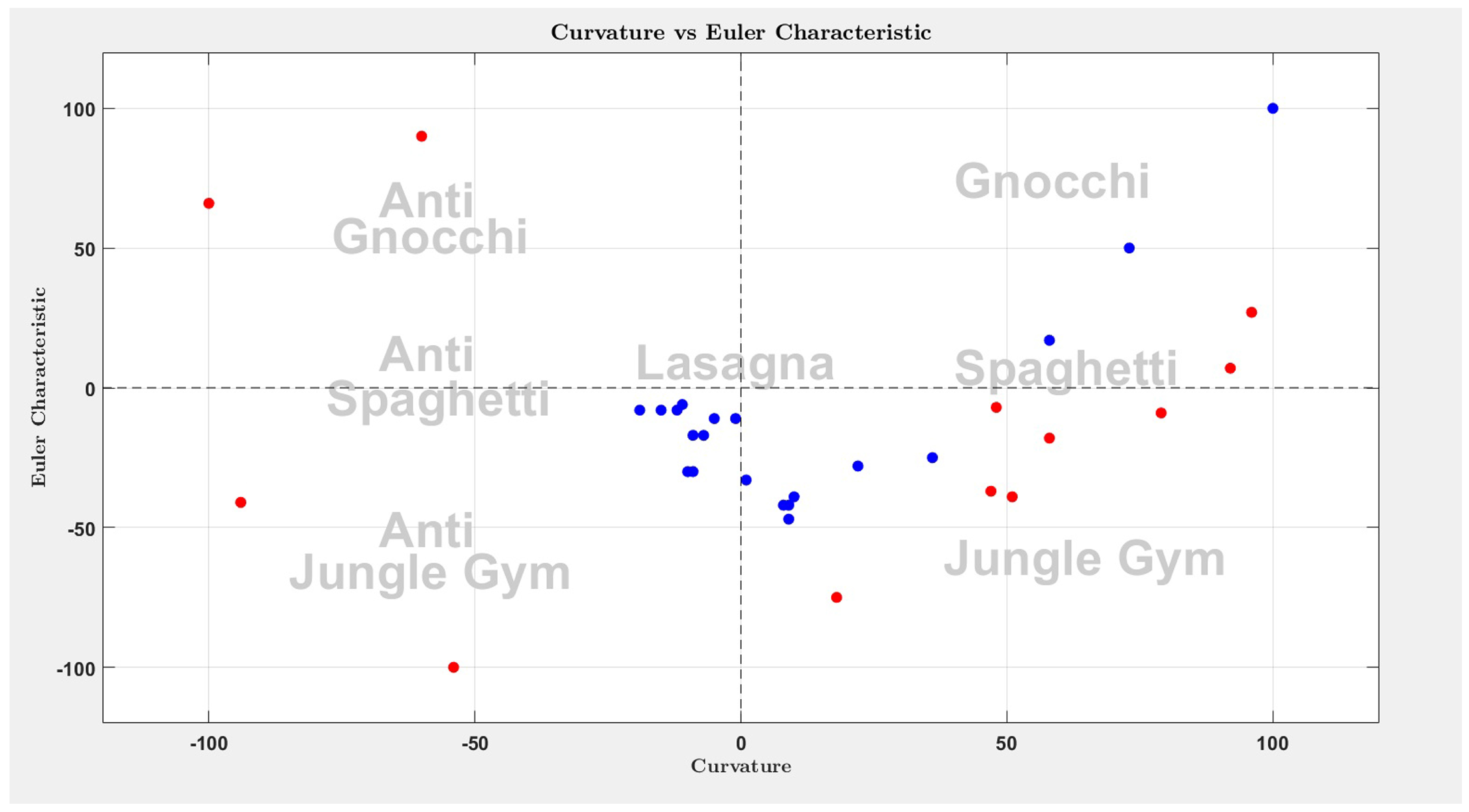
Figure 2.
Set of points of a computer generated lasagna (left), and the bodies obtained by the alpha shape method (center) and the voxelization (right).
Figure 2.
Set of points of a computer generated lasagna (left), and the bodies obtained by the alpha shape method (center) and the voxelization (right).
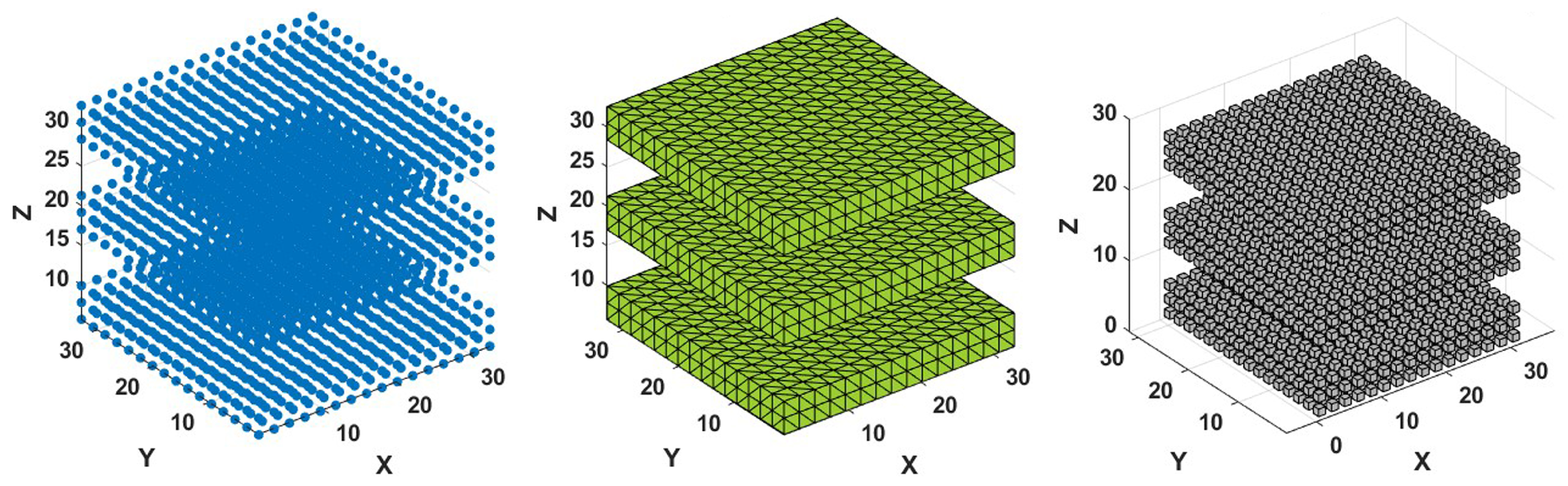
Figure 3.
Minkowski functionals calculated for the alpha shape obtained with varying alpha values (left), and for the voxelized figure with varying voxel sizes (right).
Figure 3.
Minkowski functionals calculated for the alpha shape obtained with varying alpha values (left), and for the voxelized figure with varying voxel sizes (right).
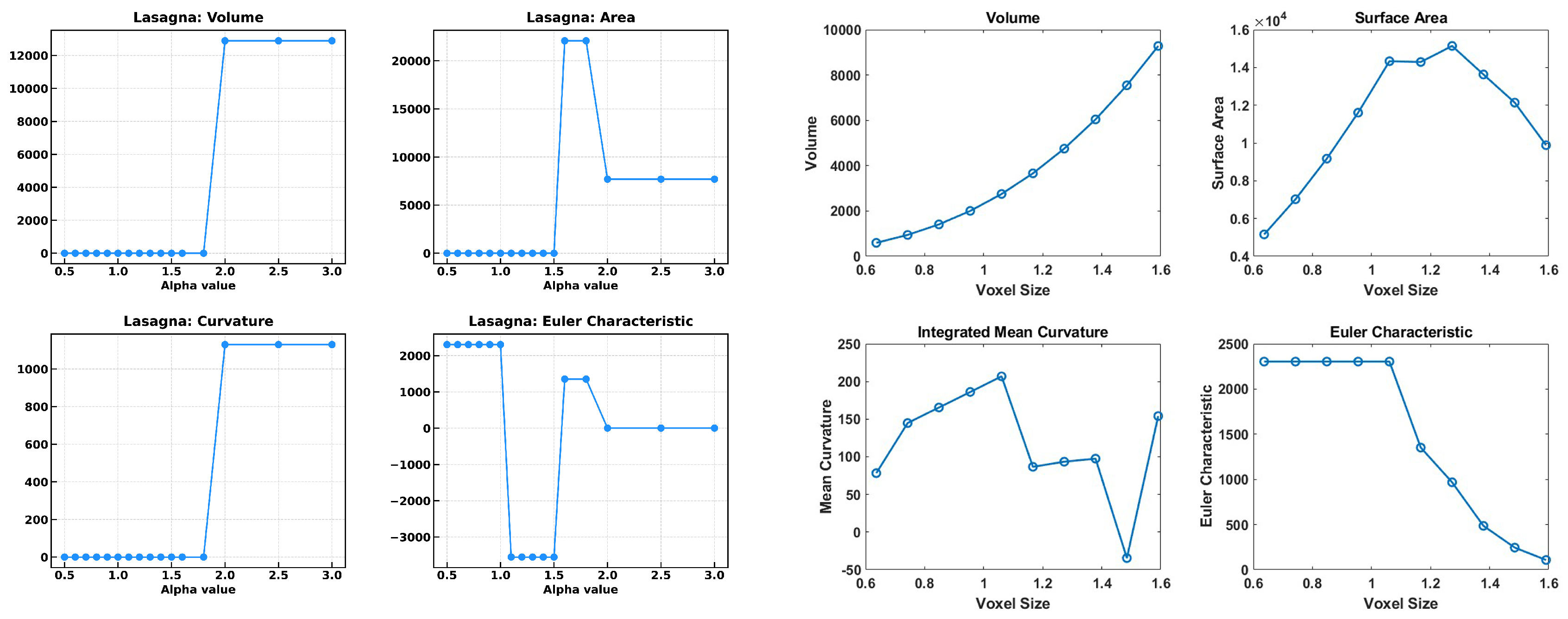
Figure 4.
Left: Set of points of a lasagna obtained by a molecular dynamics study of a system with 4000 particles thermalized at MeV, , and . Right: Alpha shape of the point set obtained with an alpha value of 2.0 fm.
Figure 4.
Left: Set of points of a lasagna obtained by a molecular dynamics study of a system with 4000 particles thermalized at MeV, , and . Right: Alpha shape of the point set obtained with an alpha value of 2.0 fm.
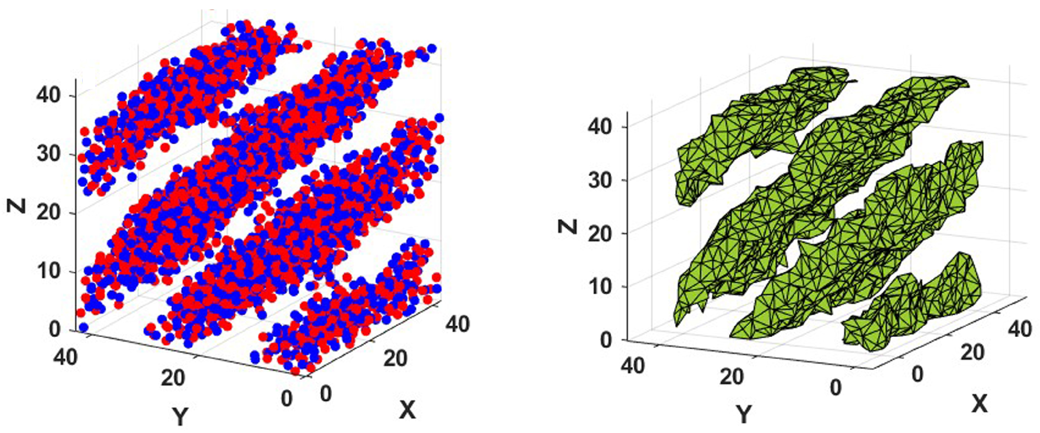
Figure 5.
Left: Minkowski Functionals of the alpha shapes solid obtained from the set of points of Figure 4 as a function of the alpha value (in fm). Right: Minkowski Functionals of the set of points of Figure 4 voxelized as a function of the voxel size (in fm).
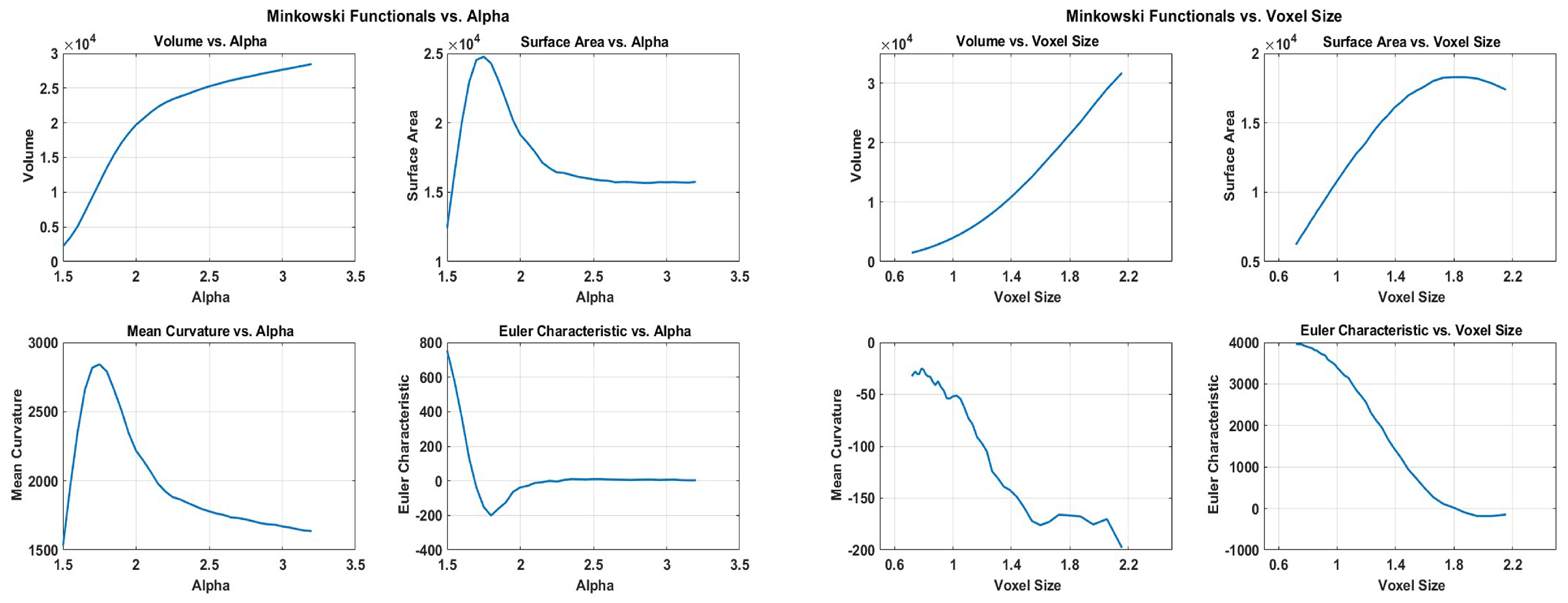
Figure 6.
Nuclear matter structures for MeV.
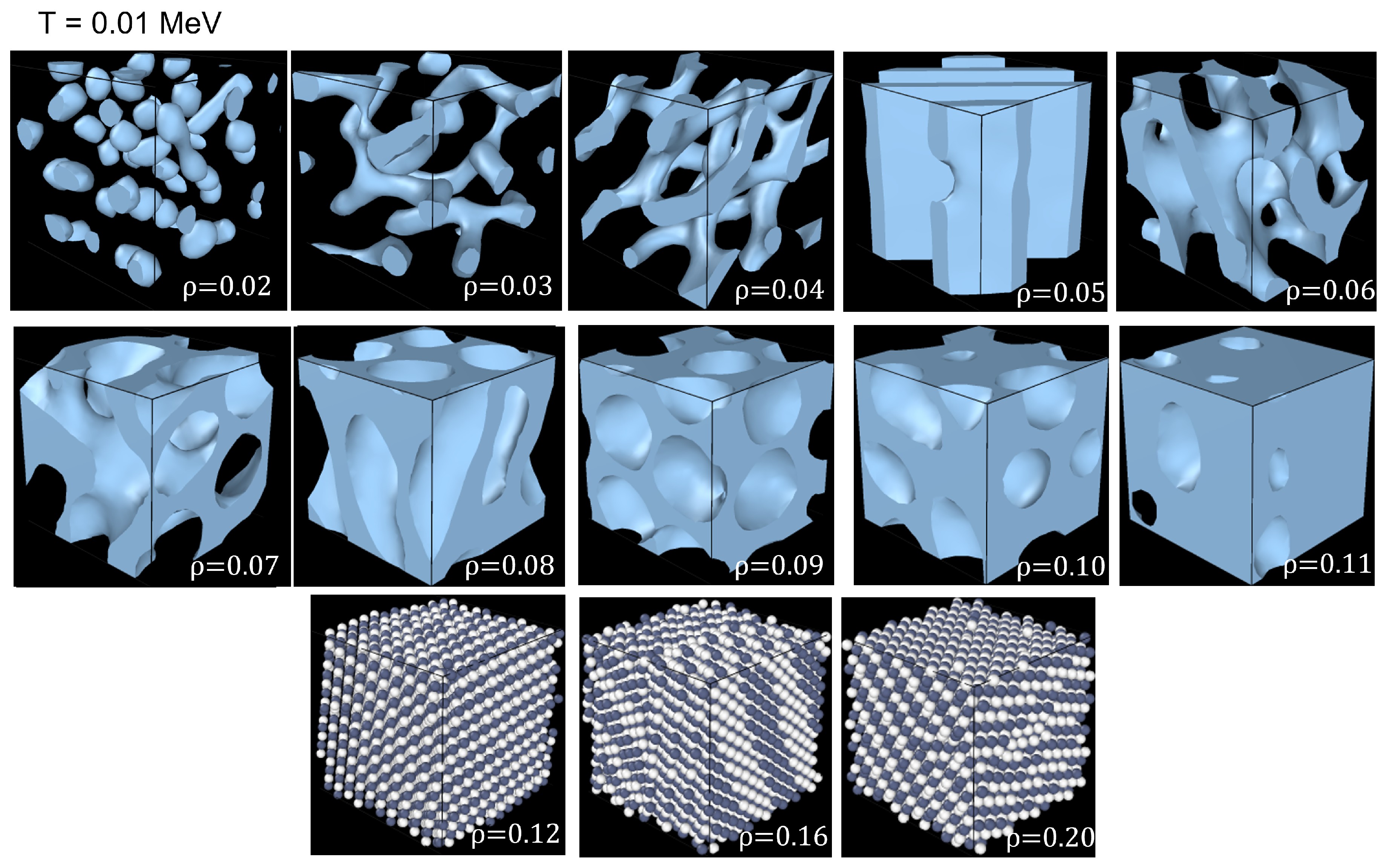
Figure 7.
Nuclear matter structures for MeV.
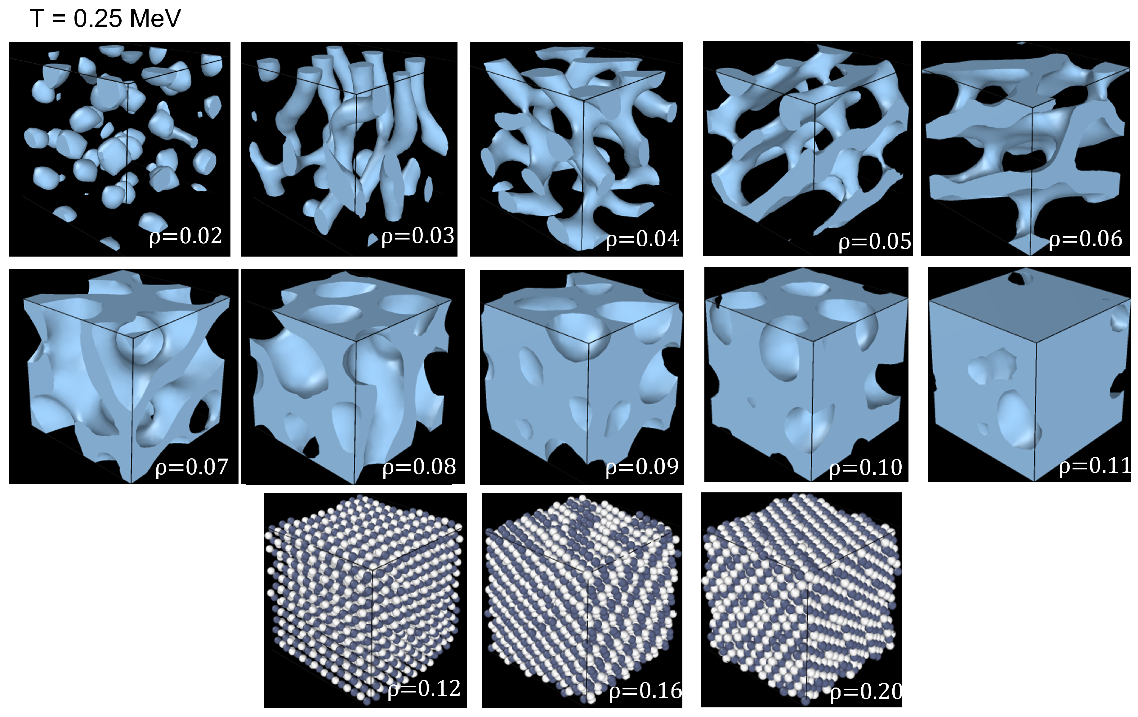
Figure 8.
Nuclear matter structures for MeV.
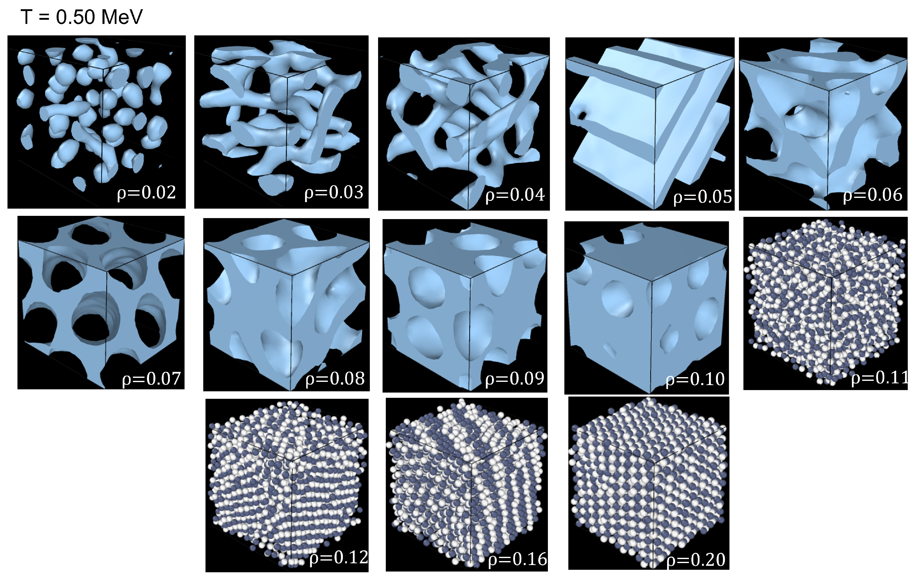
Figure 9.
Nuclear matter structures for MeV.
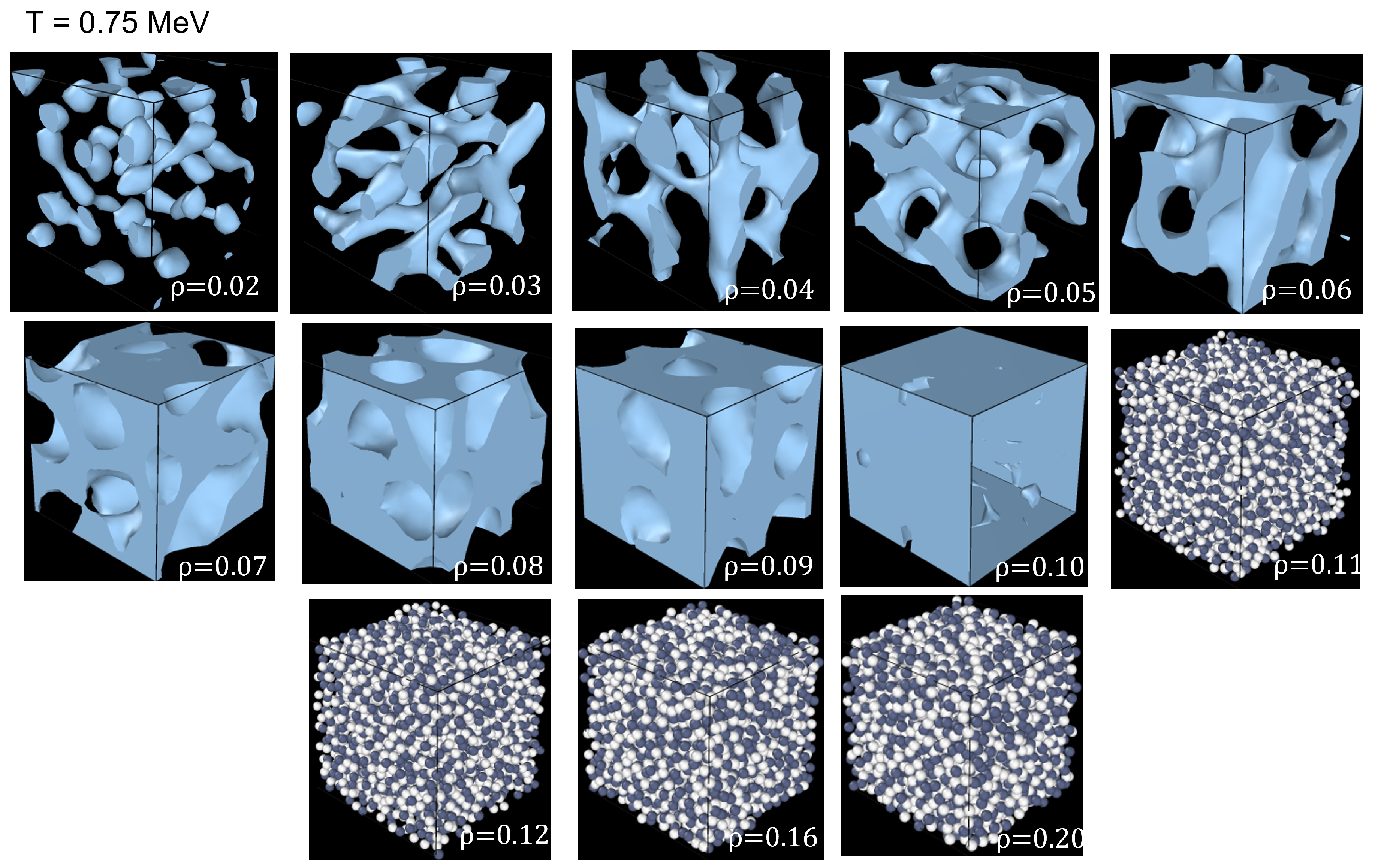
Figure 10.
Nuclear matter structures for MeV.
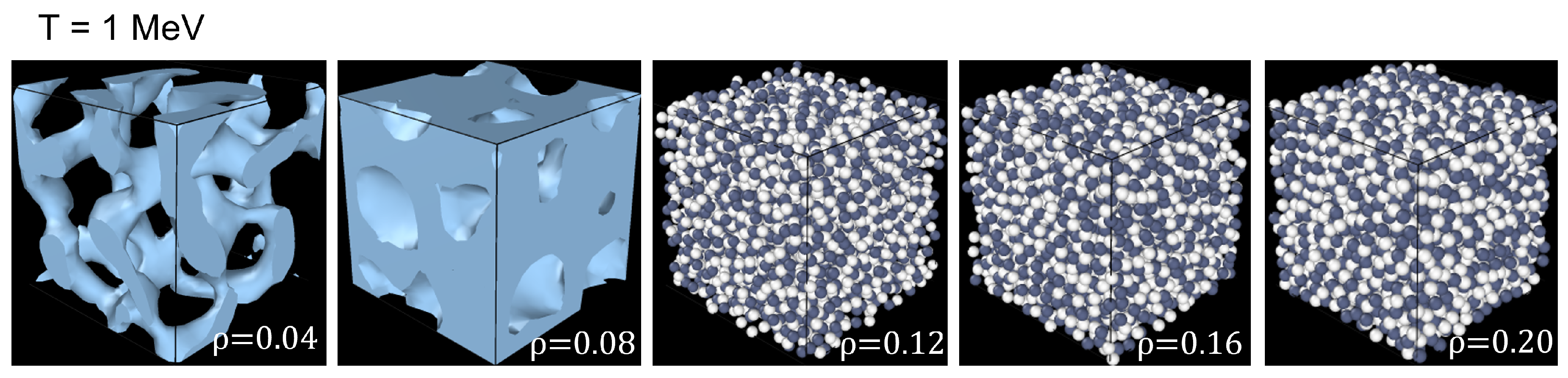
Figure 11.
Left panel: Curvature - Euler characteristic coordinates of the pastas of figures to color coded according to the structures observed visually. Right panel: expanded view of the left panel color coded according to the density.
Figure 11.
Left panel: Curvature - Euler characteristic coordinates of the pastas of figures to color coded according to the structures observed visually. Right panel: expanded view of the left panel color coded according to the density.
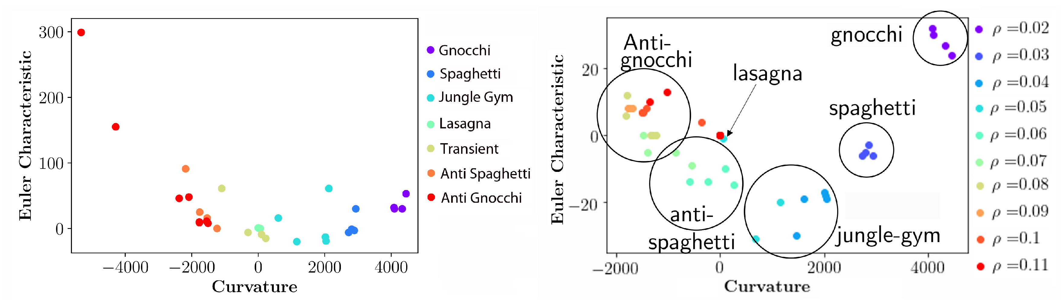
Figure 12.
Left : Side view of a set of points filling uniformly a cube but excluding a sphere at the center of the cube. Right: corresponding alpha complex.
Figure 12.
Left : Side view of a set of points filling uniformly a cube but excluding a sphere at the center of the cube. Right: corresponding alpha complex.
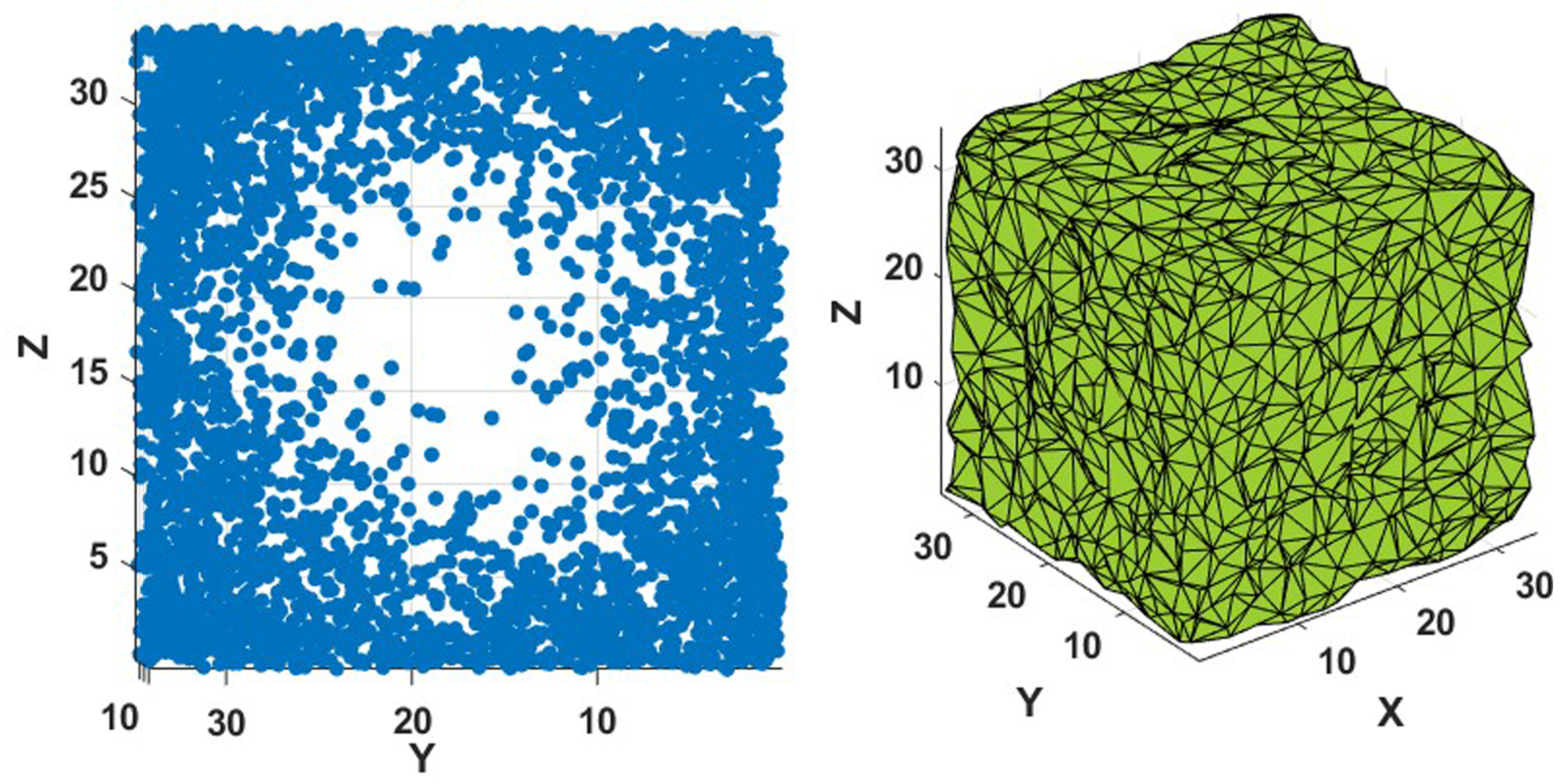
Figure 13.
Minkowski functionals of the alpha complex of a set of points filling uniformly a cube but excluding a sphere at the center of the cube, as a function of the alpha value.
Figure 13.
Minkowski functionals of the alpha complex of a set of points filling uniformly a cube but excluding a sphere at the center of the cube, as a function of the alpha value.
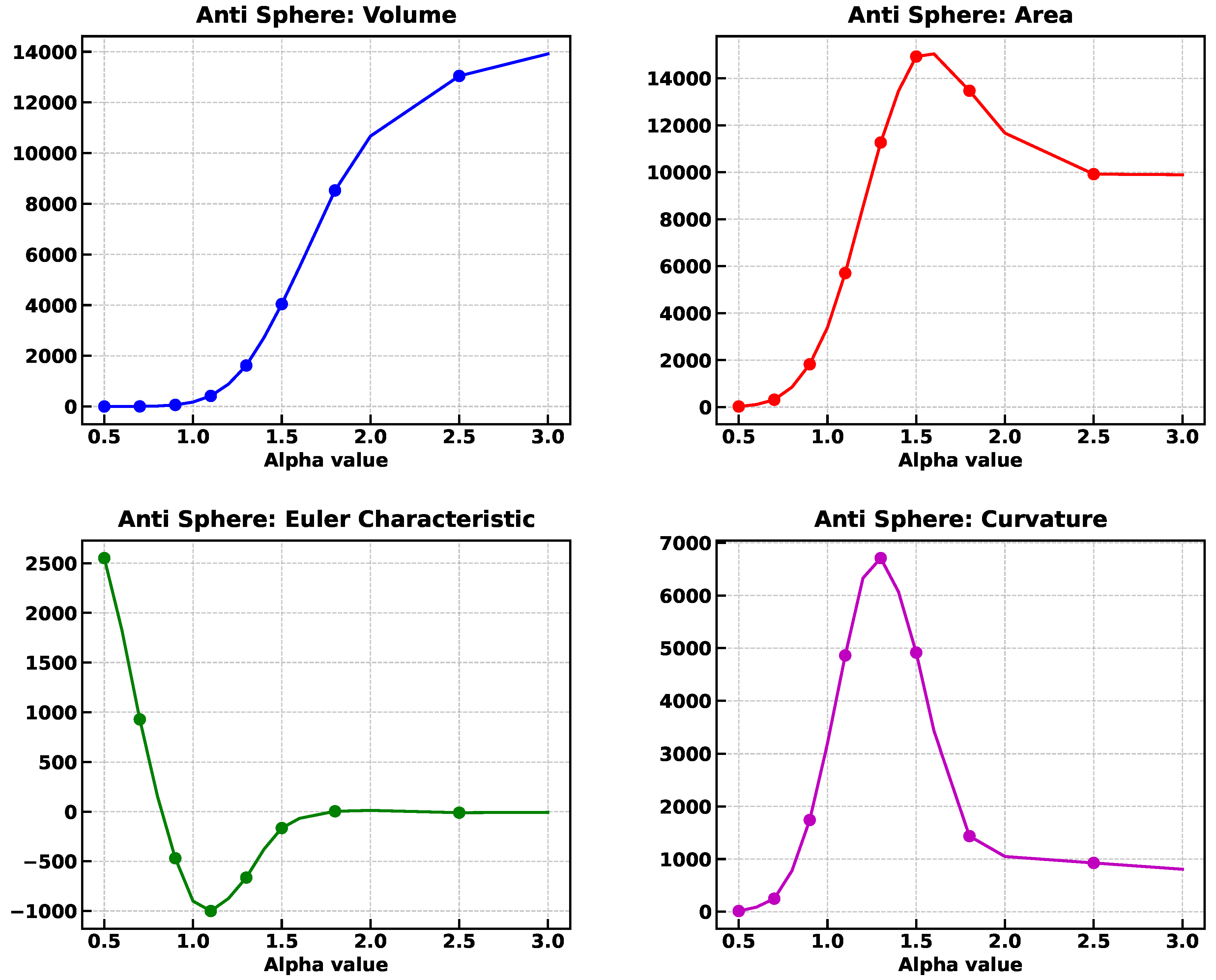
Figure 14.
Left: Side view of a set of points filling uniformly a cube but excluding a sphere at the center of the cube. Right: corresponding alpha complex.
Figure 14.
Left: Side view of a set of points filling uniformly a cube but excluding a sphere at the center of the cube. Right: corresponding alpha complex.
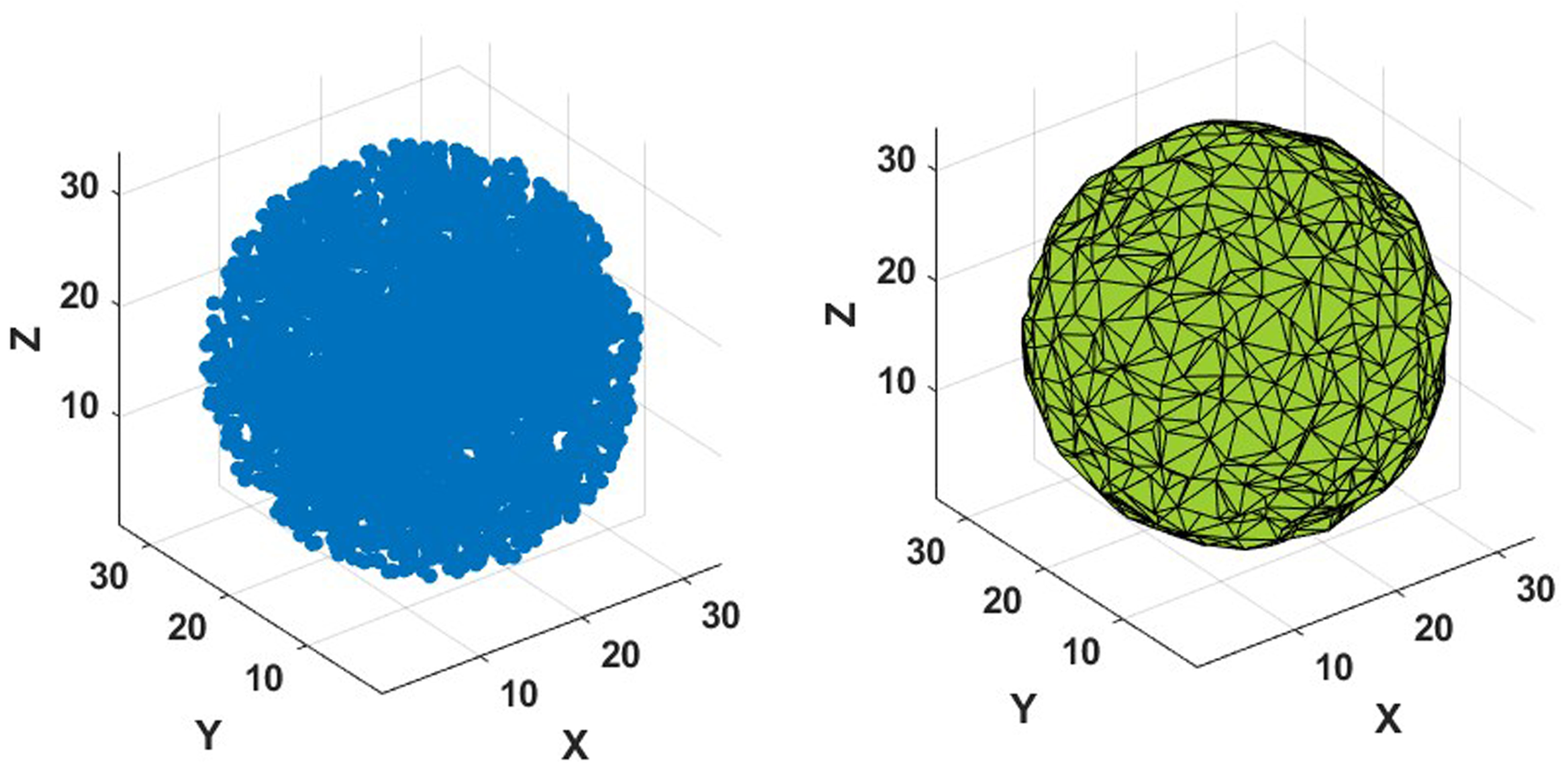
Figure 15.
Minkowski functionals of the alpha complex of a set of points filling uniformly a cube but excluding a sphere at the center of the cube, as a function of the alpha value.
Figure 15.
Minkowski functionals of the alpha complex of a set of points filling uniformly a cube but excluding a sphere at the center of the cube, as a function of the alpha value.
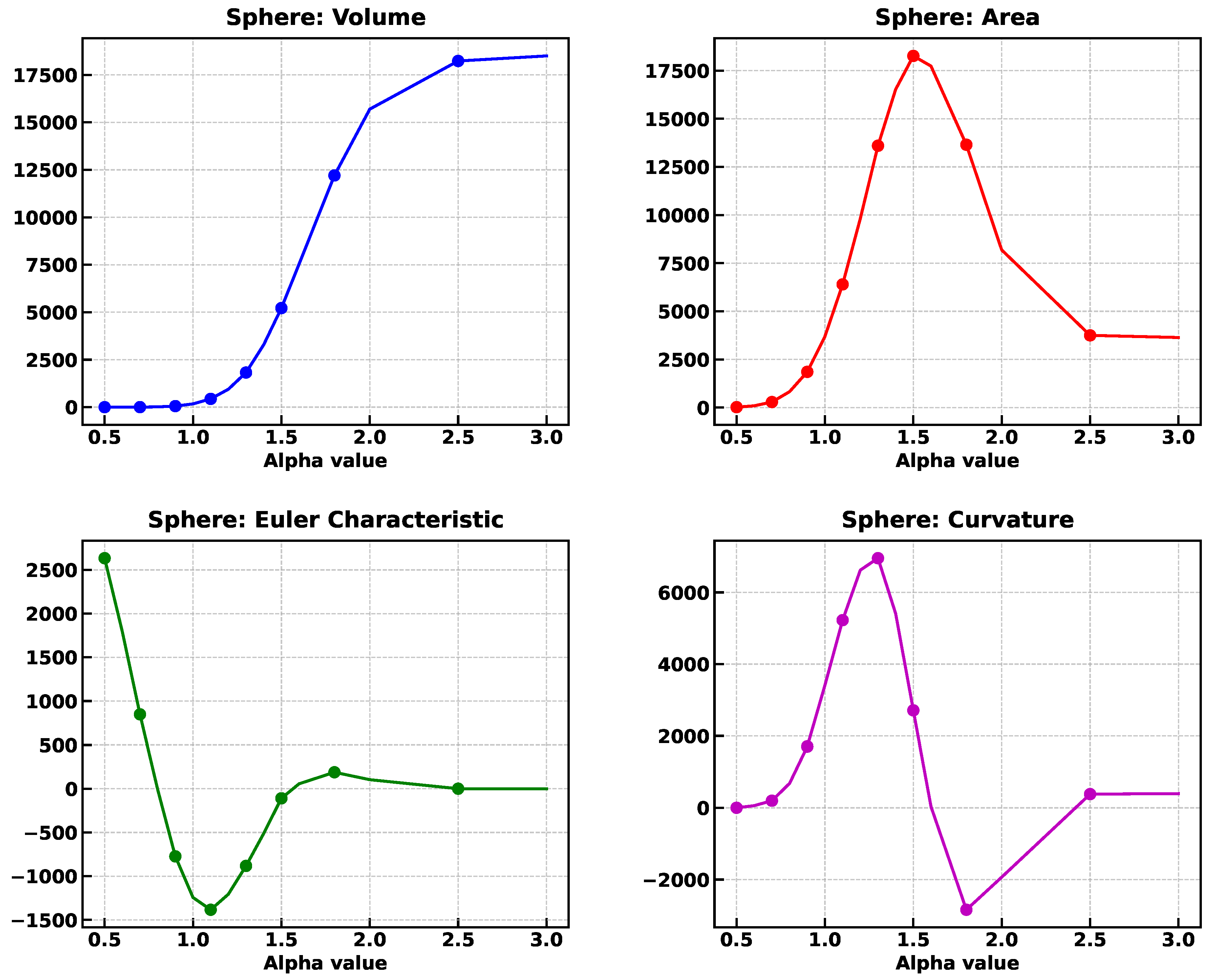
Figure 16.
Left: Side view of a set of points filling uniformly a cube but excluding eight spheres placed symmetrically in the cube in the locations indicated by the circles. Right: corresponding alpha complex.
Figure 16.
Left: Side view of a set of points filling uniformly a cube but excluding eight spheres placed symmetrically in the cube in the locations indicated by the circles. Right: corresponding alpha complex.
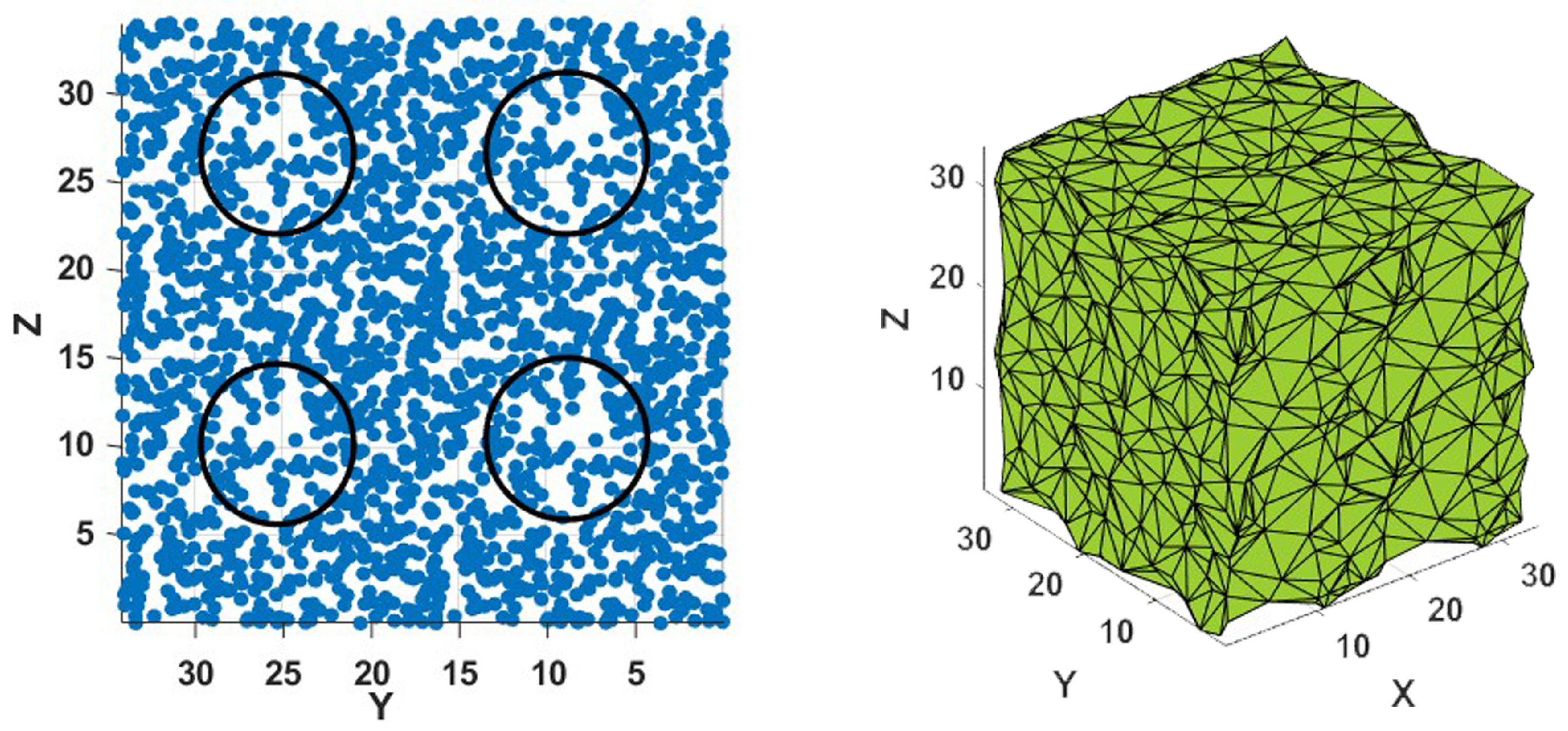
Figure 17.
Minkowski functionals of the alpha complex of a set of points filling uniformly a cube but excluding eight spheres placed symmetrically in the cube, as a function of the alpha value.
Figure 17.
Minkowski functionals of the alpha complex of a set of points filling uniformly a cube but excluding eight spheres placed symmetrically in the cube, as a function of the alpha value.
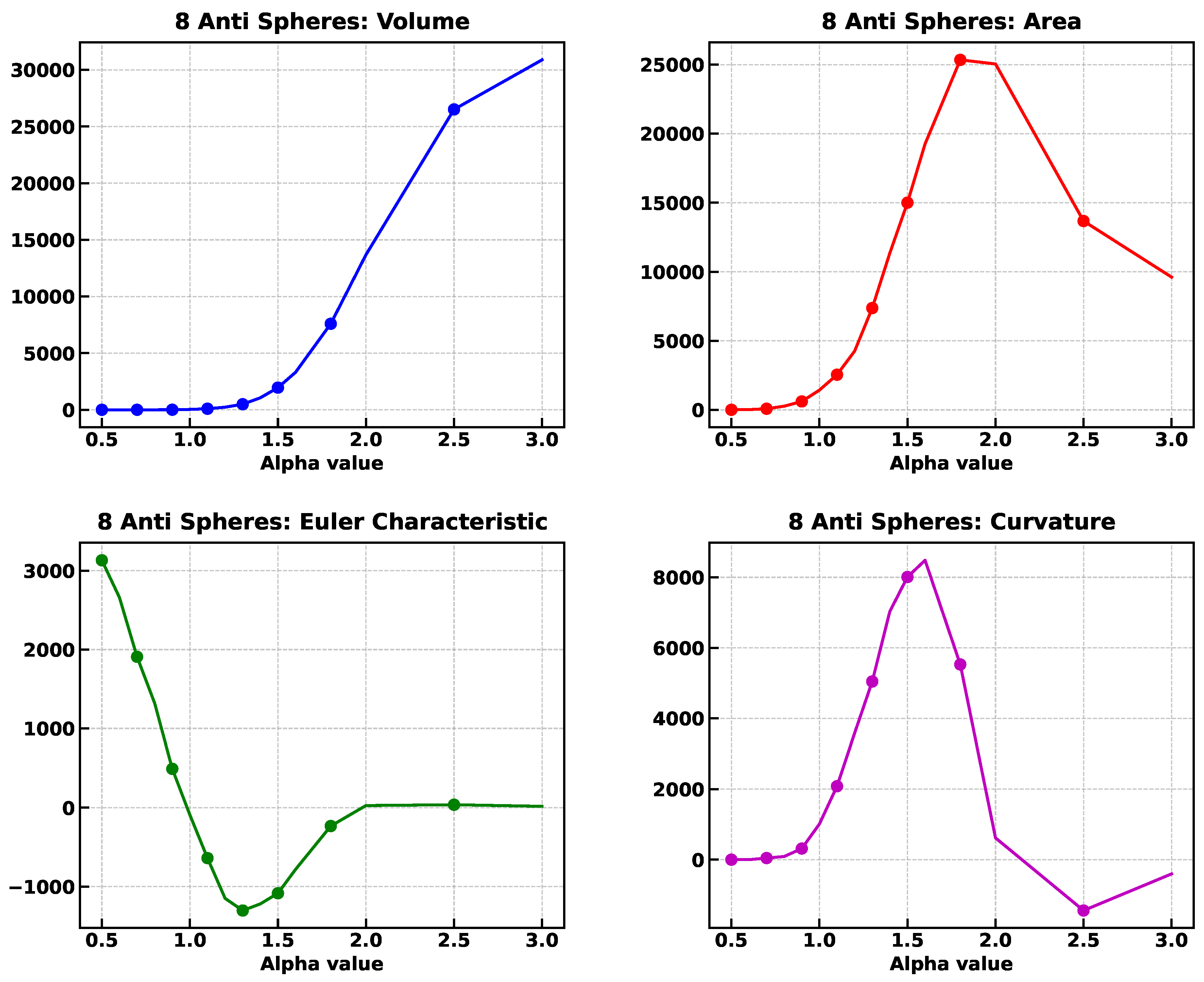
Figure 18.
Left: Set of points filling uniformly eight spheres. Right: corresponding alpha complex.
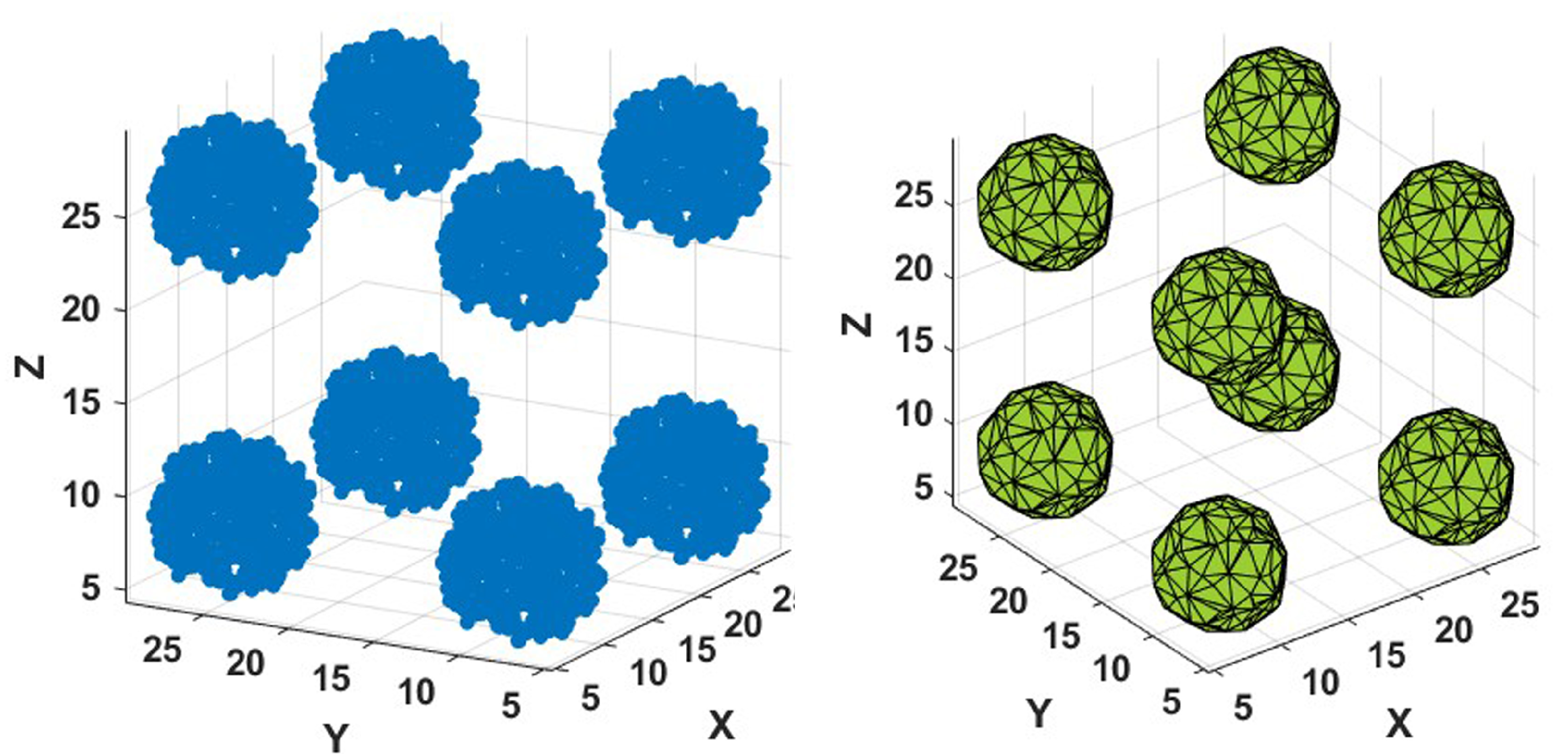
Figure 19.
Minkowski functionals of the alpha complex of a set of points filling uniformly eight spheres, as a function of the alpha value.
Figure 19.
Minkowski functionals of the alpha complex of a set of points filling uniformly eight spheres, as a function of the alpha value.
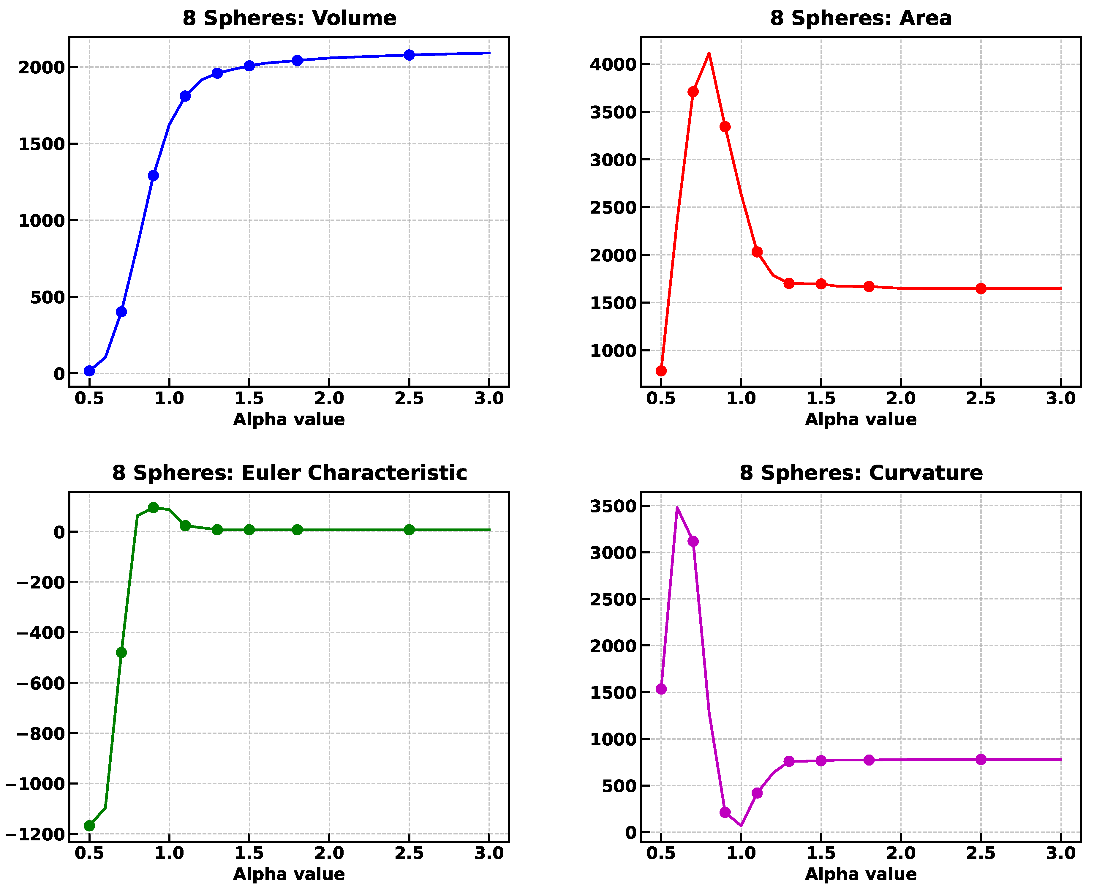
Figure 20.
Left: Set of points filling uniformly four tubes. Right: corresponding alpha complex.
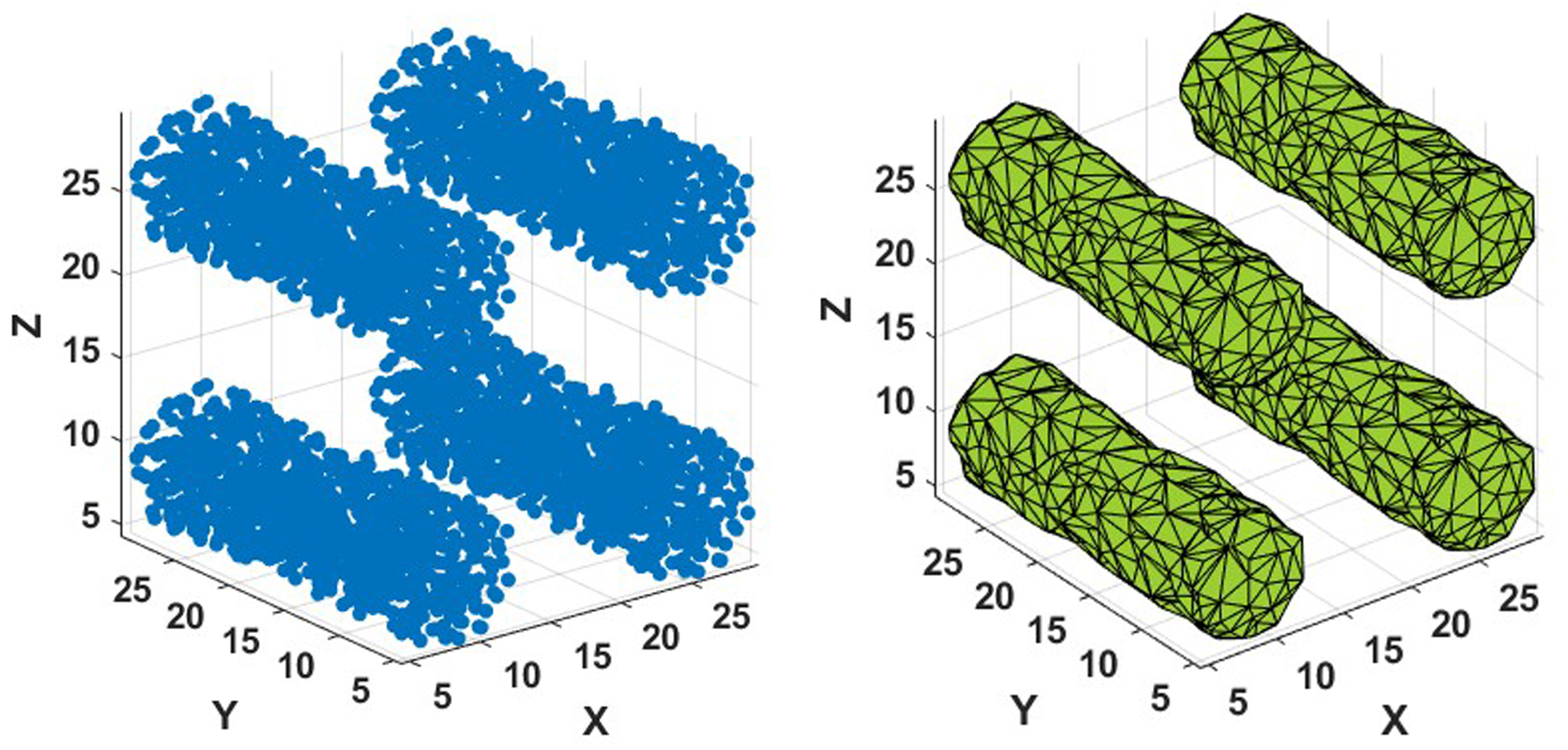
Figure 21.
Minkowski functionals of the alpha complex of a set of points filling uniformly four tubes, as a function of the alpha value.
Figure 21.
Minkowski functionals of the alpha complex of a set of points filling uniformly four tubes, as a function of the alpha value.
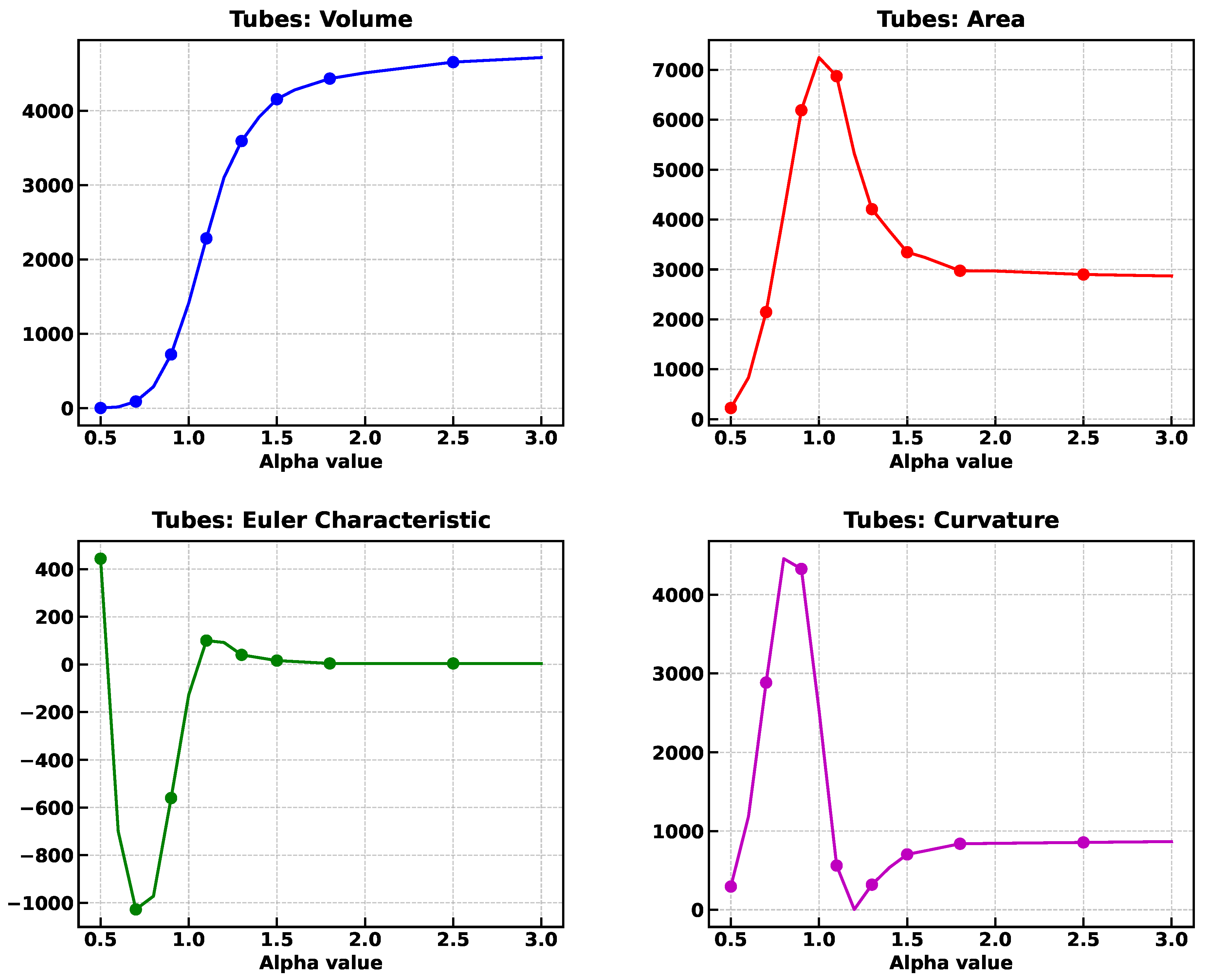
Figure 22.
Left: Set of points filling uniformly a cube except for the location of four tubes. Right: corresponding alpha complex for .
Figure 22.
Left: Set of points filling uniformly a cube except for the location of four tubes. Right: corresponding alpha complex for .
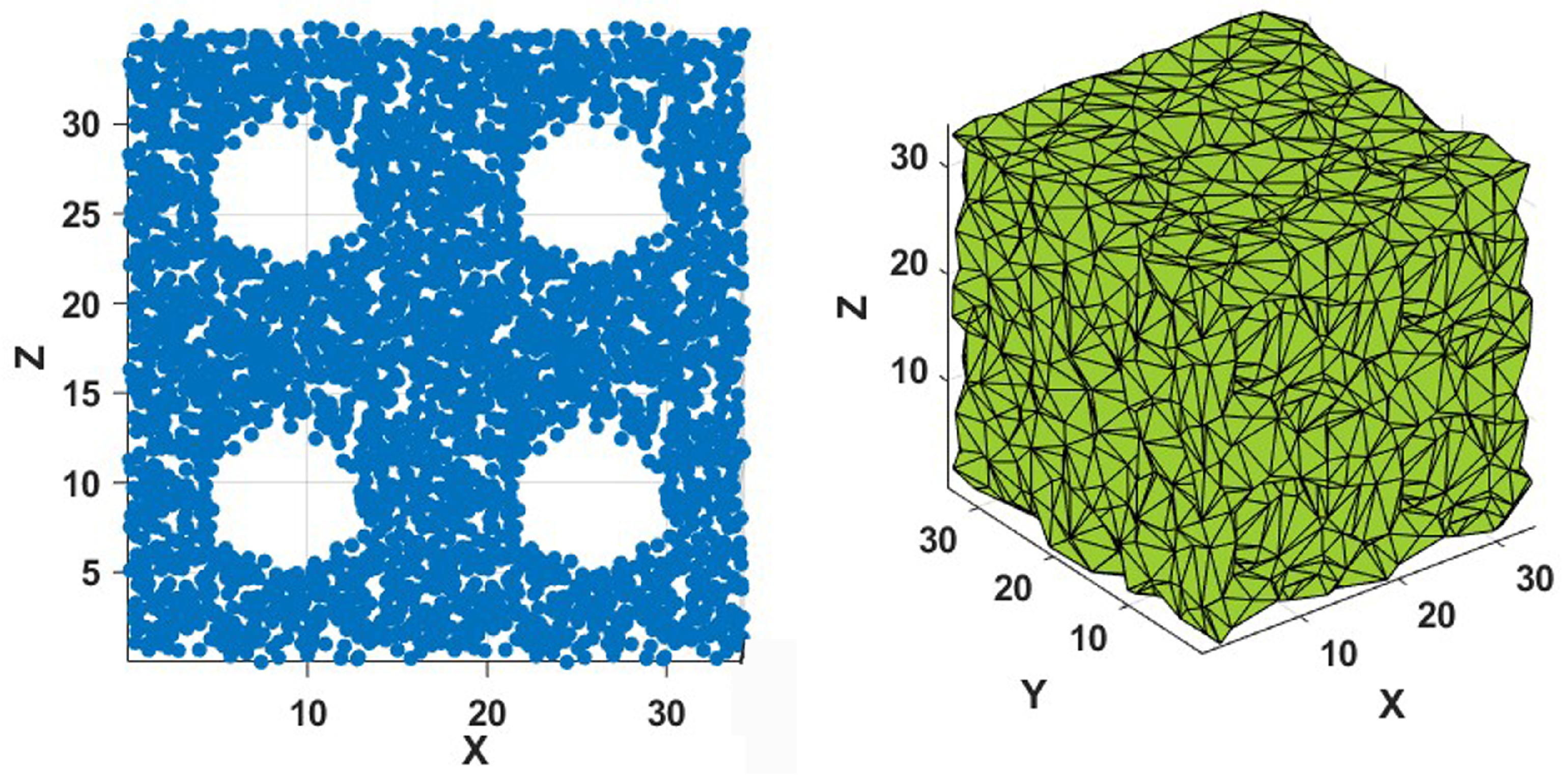
Figure 23.
Minkowski functionals of the alpha complex of Figure 22, as a function of the alpha value.
Figure 23.
Minkowski functionals of the alpha complex of Figure 22, as a function of the alpha value.
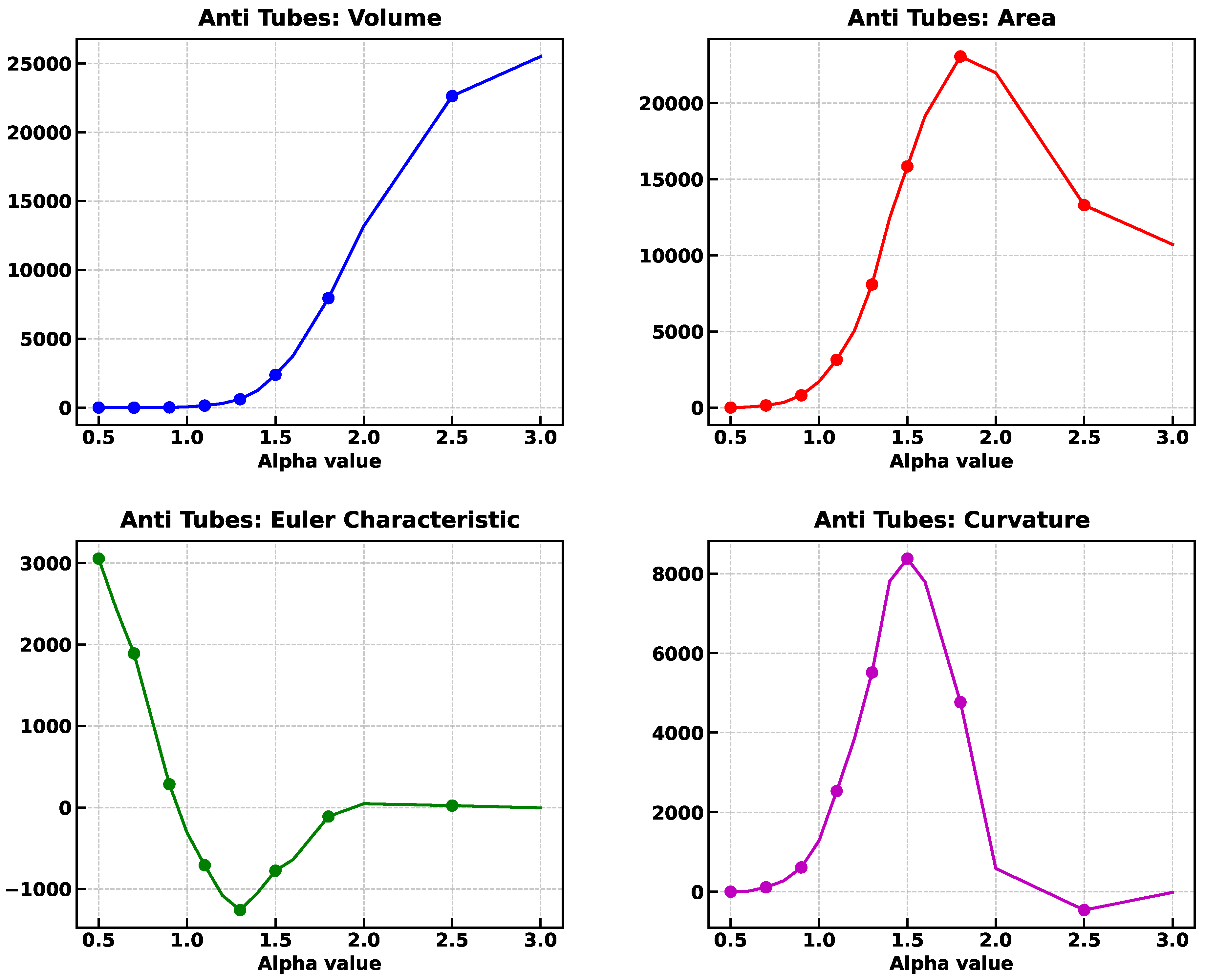
Figure 24.
Left: Set of points filling uniformly a sphere at the center of the cube. Right: corresponding alpha complex.
Figure 24.
Left: Set of points filling uniformly a sphere at the center of the cube. Right: corresponding alpha complex.
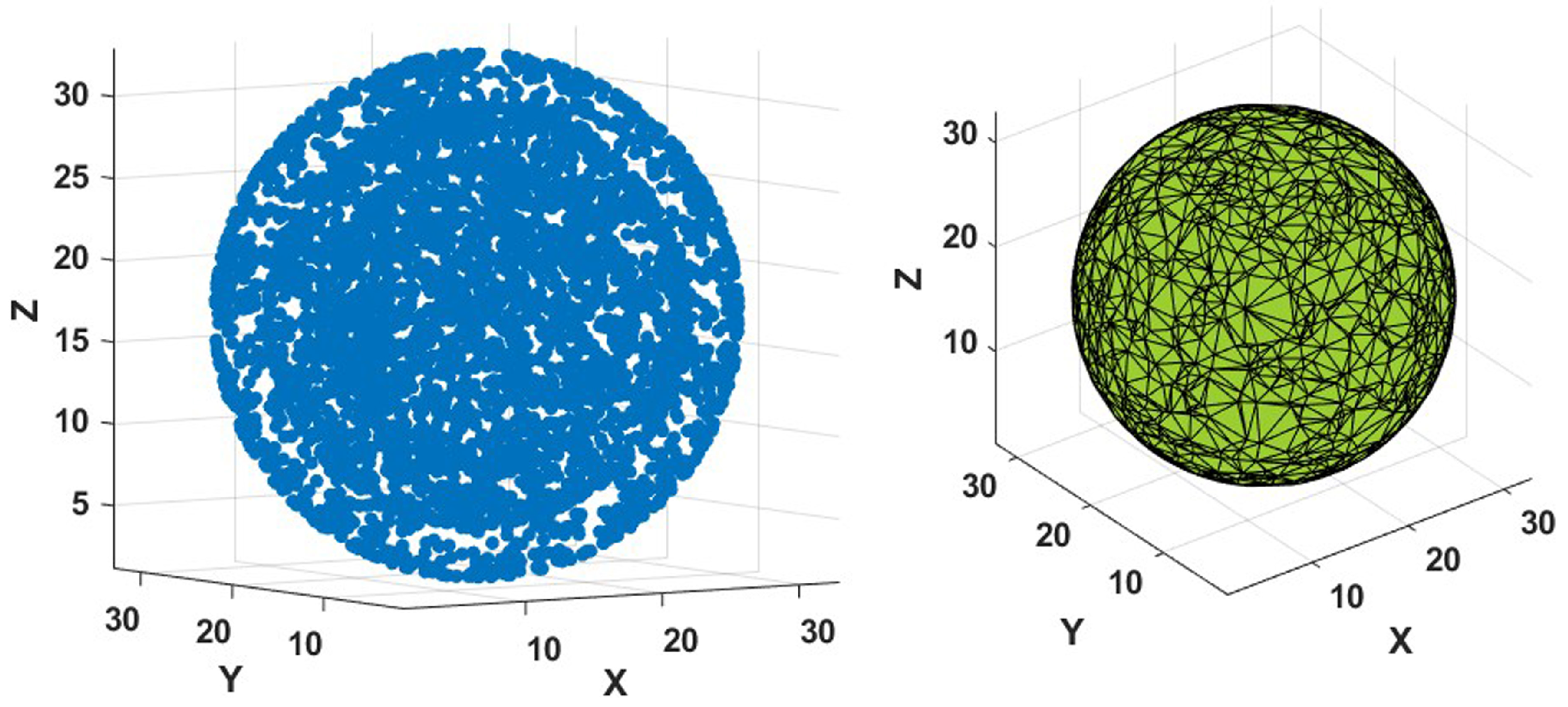
Figure 25.
Minkowski functionals of the alpha complex of a set of points filling uniformly a sphere, as a function of the alpha value.
Figure 25.
Minkowski functionals of the alpha complex of a set of points filling uniformly a sphere, as a function of the alpha value.
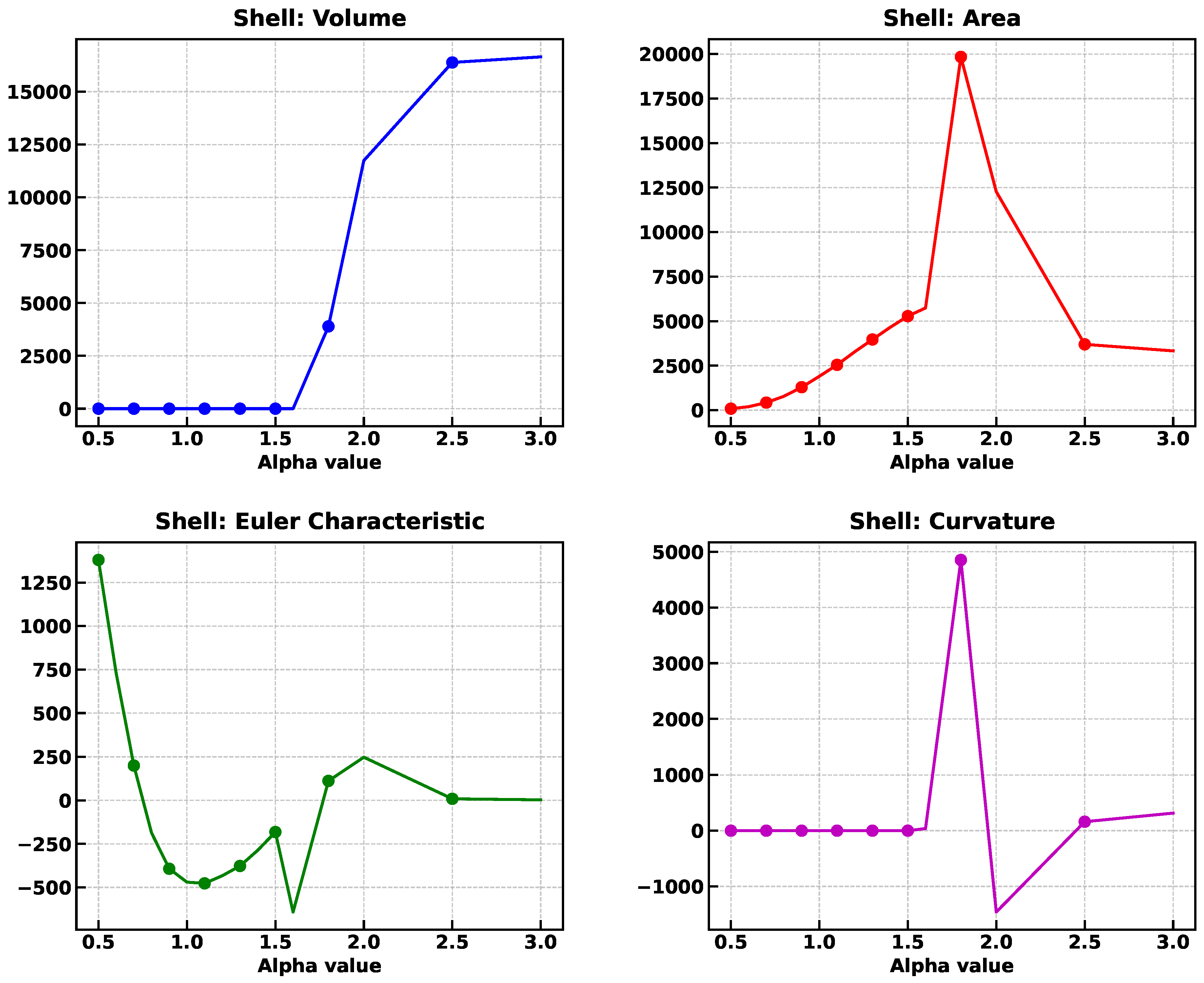
Figure 26.
Curvature-Euler Characteristic for the test structures.
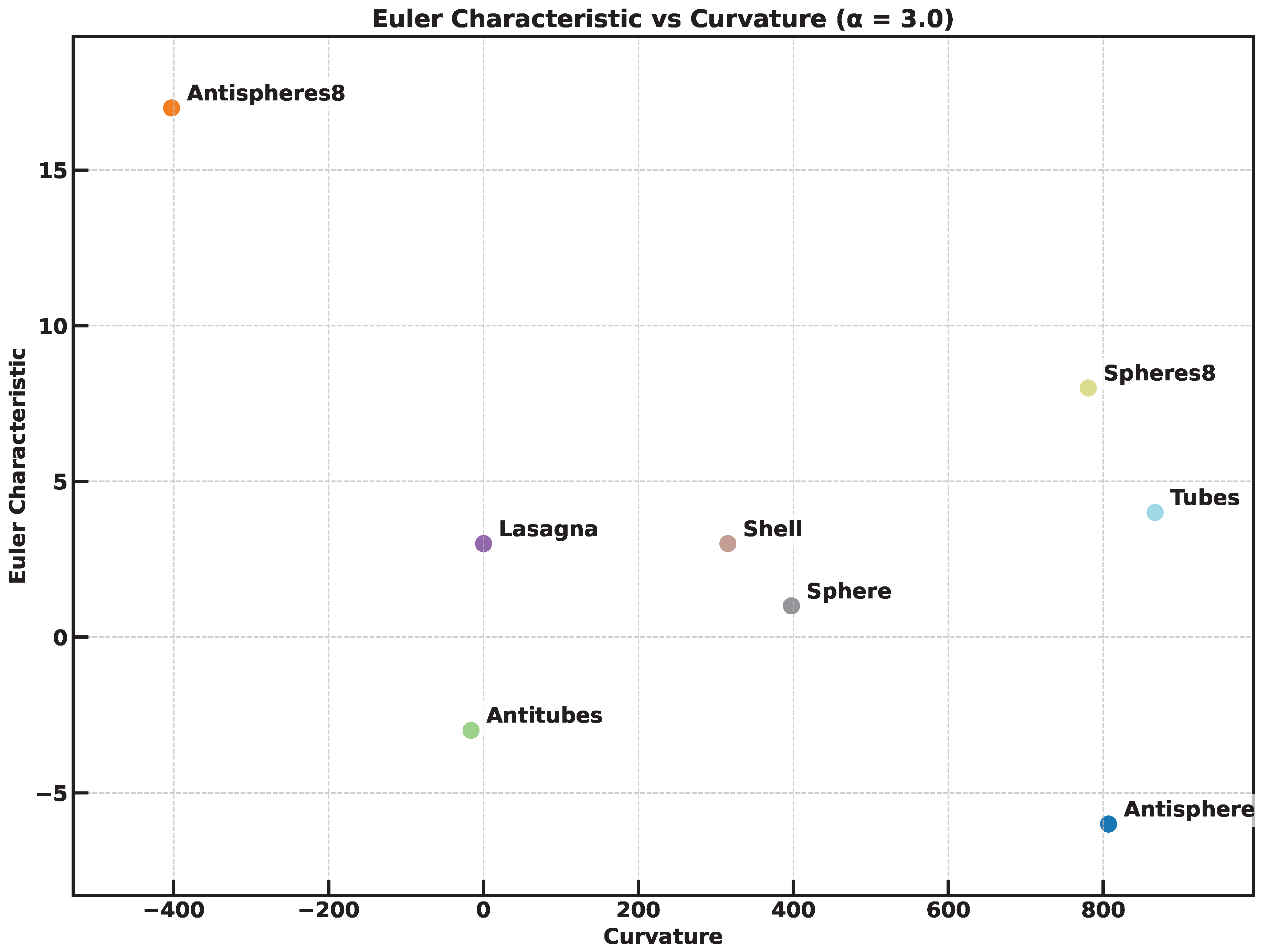

Table 1.
Minkowski functionals for the solids of Figure 2.
Table 1.
Minkowski functionals for the solids of Figure 2.
| Minkowski Functional | Estimated value | Voxels | Alpha shape |
|---|---|---|---|
| (voxel size 1.06 fm) | (alpha 3.0 fm) | ||
| Volume (fm) | 13,649 | 2,750 | 12,889 |
| Area (fm) | 7,791 | 14,330 | 7,696 |
| Mean curvature (fm) | 0 | 207 | 1,129 (0.146) |
| Euler Characteristic | 2 | 2304 | 0 |
Table 2.
Minkowski functionals for the voxelization and alpha shape of Figure 4.
Table 2.
Minkowski functionals for the voxelization and alpha shape of Figure 4.
| Minkowski Functional | Voxels | Alpha shape |
|---|---|---|
| (voxel size 1.8 fm) | (alpha 2.0 fm) | |
| Volume | 21,327 | 19,730 |
| Area | 18,283 | 19,146 |
| Mean curvature | -166.63 | 2,216 |
| Euler Characteristic | 23 | -38 |
Table 3.
Parameter set for the CMD computations [6].
Table 3.
Parameter set for the CMD computations [6].
| Parameter | Pandharipande | New Medium | Units |
|---|---|---|---|
| 3088.118 | 3097.0 | MeV | |
| 2666.647 | 2696.0 | MeV | |
| 373.118 | 379.5 | MeV | |
| 1.7468 | 1.648 | fm | |
| 1.6000 | 1.528 | fm | |
| 1.5000 | 1.628 | fm | |
| 5.4 | 5.4/20 | fm |
Disclaimer/Publisher’s Note: The statements, opinions and data contained in all publications are solely those of the individual author(s) and contributor(s) and not of MDPI and/or the editor(s). MDPI and/or the editor(s) disclaim responsibility for any injury to people or property resulting from any ideas, methods, instructions or products referred to in the content. |
© 2025 by the authors. Licensee MDPI, Basel, Switzerland. This article is an open access article distributed under the terms and conditions of the Creative Commons Attribution (CC BY) license (http://creativecommons.org/licenses/by/4.0/).
Copyright: This open access article is published under a Creative Commons CC BY 4.0 license, which permit the free download, distribution, and reuse, provided that the author and preprint are cited in any reuse.


