Deep Reinforcement Learning Based Robotic Arm’s Target Reaching Performance Enhancement

1. Introduction

The enhancement of precision for robot arm manipulation remains a core research area for acquiring full autonomy of robots in various sectors such as industrial manufacturing and assembly processes. The next logical progression in this field is to achieve complete autonomy of robotic manipulators through the use of machine learning (ML), artificial neural networks (ANNs), and artificial intelligence (AI) as a whole, given the maturity of image recognition and vision systems [1,2]. Numerous attempts have been made to create intelligent robots that can take tasks and execute accordingly [3,4,5,6,7,8,9,10].

Although developing a system with intelligence close to that of humans is still a long way off, robots that can perform specialized autonomous activities, such as intelligent facial emotion recognition [11], fly in natural and man-made environments [12], drive a vehicle [13], swim [14], carry boxes and material in different terrains [15], and pick up and place objects [16,17] is already actualized.

However, some challenges must be overcome to achieve this goal. For instance, the mapping complexity from Cartesian space to the joint space of a robot arm increases with the number of joints and linkages that the manipulator has. This is problematic because the tasks assigned to a robotic arm are in Cartesian space, whereas the commands (velocity or torque) are in joint space [18,19]. Therefore, if full autonomy of robotic manipulators is the objective, the target-reaching problem is probably one of the most crucial factors that must be addressed.

The field of reinforcement learning, as described in [20,21], is a type of machine learning that aims to maximize the outcome of a given system using a dynamic and autonomous trial-and-error approach. It shares a similar objective with human intelligence, which is characterized by the ability to perceive and retain information as knowledge to be used for environment-adaptive behaviors. Central to the reinforcement learning framework are trial-and-error search and delayed rewards, which allow the learning strategy to interact with the environment by performing actions and discovering rewards [22]. Through this approach, software agents and machines can automatically select the most effective course of action to take in a given circumstance, thus improving performance. Reinforcement learning offers a framework and set of tools for designing sophisticated and challenging-to-engineer behaviors in robotics [23,24]. In contrast, the challenges presented by robotic issues serve as motivation, impact, and confirmation of advances in reinforcement learning. Multiple previous works on the implementation of reinforcement learning in the field of robotics depict this fact [25,26,27,28,29].

2. Modeling of Robotic Arm

2.1. Direct Kinematic Model of Robot Arm

The rotation matrices in the DH coordinate frame represent the rotations about the X and Z axes. The rotation matrices for these axes are, respectively, given as:

$$R_x=\left[\begin{array}{ccc}1& 0& 0\\ 0& C{\delta }_i& -S{\delta }_i\\ 0& S{\delta }_i& C{\delta }_i\end{array}\right]$$

(1)

and

$$R_z=\left[\begin{array}{ccc}C{\varphi }_i& -S{\varphi }_i& 0\\ S{\varphi }_i& C{\varphi }_i& 0\\ 0& 0& 1\end{array}\right]$$

(2)

The homogeneous transformation matrix ($T_{i-1}^i$) that accounts for rotation and translation is given as:

$$\begin{array}{cc}\hfill T_{i-1}^i& =\left[\begin{array}{cc}{R}_{i-1}^1& p_{i-1}^1\\ 0& 1\end{array}\right]\hfill \\ & ={\mathrm{Rot}}_x\left({\varphi }_i\right)·{\mathrm{trans}}_x\left(d_i\right)·{\mathrm{trans}}_z\left({\Delta }_i\right)·{\mathrm{Rot}}_z\left(a_i\right)\hfill \end{array}$$

$$\Rightarrow \begin{array}{c}\hfill T_{i-1}^1=\left[\begin{array}{cccc}C{\varphi }_i& -S{\varphi }_{i}C{\delta }_i& S{\varphi }_{i}S{\delta }_i& a_{i}C{\varphi }_i\\ S{\varphi }_i& C{\varphi }_{i}C{\delta }_i& -C{\varphi }_{i}S{\delta }_i& a_{i}S{\varphi }_i\\ 0& S{\delta }_i& C{\delta }_i& d_i\\ 0& 0& 0& 1\end{array}\right]\end{array}$$

(3)

where:

• The rotation matrix ($R_{i-1}^1$) represents the orientation of the i-th frame relative to the $(i-1)$-th frame.
• $P_{i-1}^1$ represents the center of the link frame with components ($P_x$, $P_y$, and $P_z$).

2.1.1. DH Axis Representation

The four DH parameters describe the translation and rotation relationship between two consecutive coordinate frames as follows:

• d: a distance between the current frame and the previous frame along the Z-axis,
• ($\varphi$): an angle between the X-axis of the previous frame and the X-axis of the current frame about the previous z-axis,
• a: a distance between the Z-axes of the current and previous frames.
• $\delta$: an offset of the previous frame from the current frame along the Z-axis of the current frame.

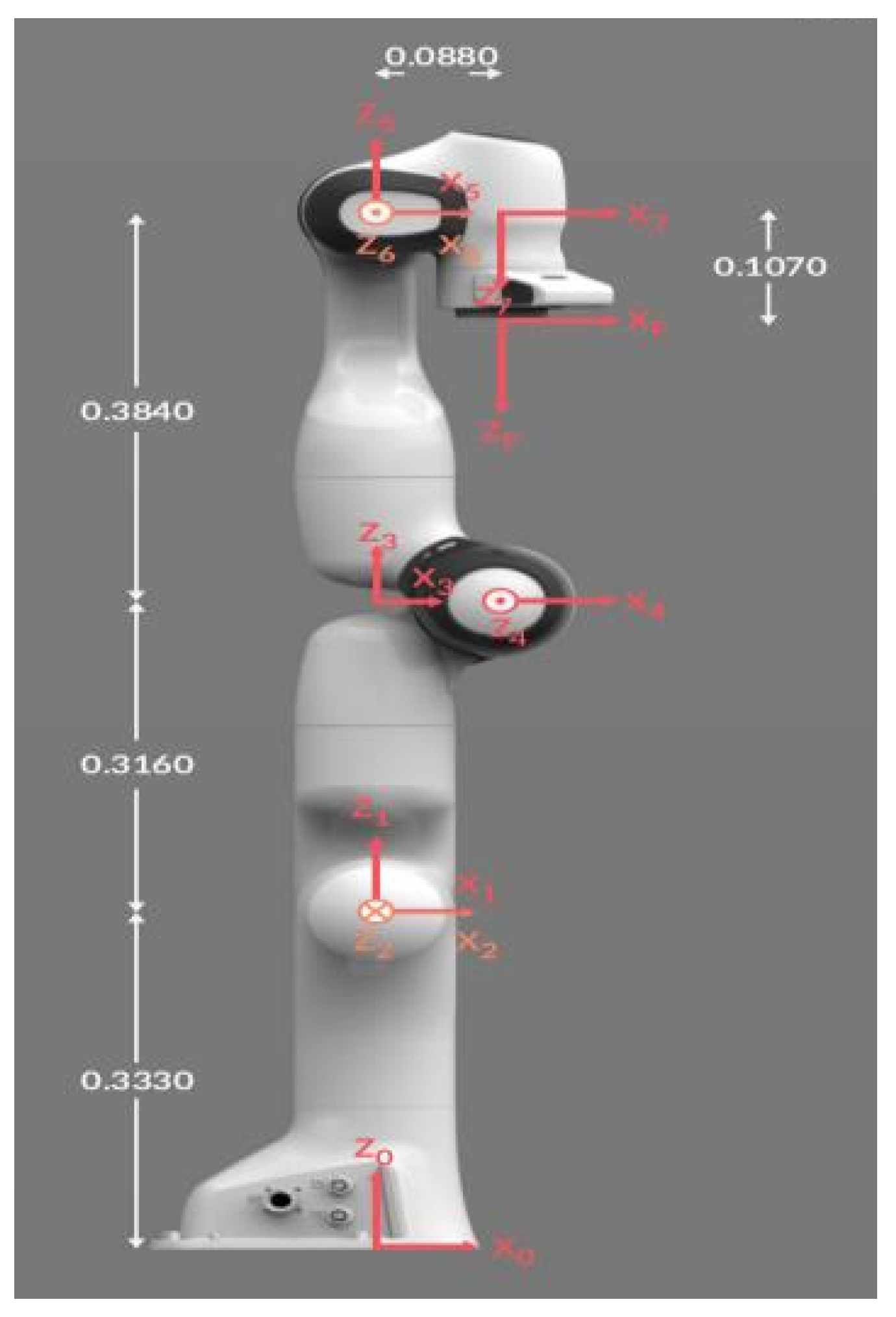
The DH parameters for the Franka Panda robot, shown in Figure 1 are given in Table 1. From the above DH parameters and based on the homogeneous transformation matrix 3, the transformation matrix for the Franka Panda robot is derived as.

$$T_{i-1}^1=\left[\begin{array}{cccc}C{\varphi }_i& -S{\varphi }_{i}C{\delta }_i& S{\varphi }_{i}S{\delta }_i& a_{i}C{\varphi }_i\\ S{\varphi }_i& C{\varphi }_{i}C{\delta }_i& -C{\varphi }_{i}S{\delta }_i& a_{i}S{\varphi }_i\\ 0& S{\delta }_i& C{\delta }_i& d_i\\ 0& 0& 0& 1\end{array}\right]$$

$$T_0^1=\left[\begin{array}{cccc}C{\varphi }_1& -S{\varphi }_1& 0& 0\\ S{\varphi }_1& C{\varphi }_1& 0& 0\\ 0& 0& 1& 0.33\\ 0& 0& 0& 1\end{array}\right]$$

(4)

$$T_1^2=\left[\begin{array}{cccc}C{\varphi }_2& 0& -S{\varphi }_2& 0\\ S{\varphi }_2& 0& C{\varphi }_2& 0\\ 0& -1& 0& 0\\ 0& 0& 0& 1\end{array}\right]$$

(5)

$$T_2^3=\left[\begin{array}{cccc}C{\varphi }_3& 0& S{\varphi }_3& 0\\ S{\varphi }_3& 0& -C{\varphi }_3& 0\\ 0& 1& 1& 0.316\\ 0& 0& 0& 1\end{array}\right]$$

(6)

$$T_3^4=\left[\begin{array}{cccc}C{\varphi }_4& 0& S{\varphi }_4& 0.0825C{\varphi }_4\\ S{\varphi }_4& 0& -C{\varphi }_4& 0.0825S{\varphi }_4\\ 0& 1& 1& 0\\ 0& 0& 0& 1\end{array}\right]$$

(7)

$$T_4^5=\left[\begin{array}{cccc}C{\varphi }_5& 0& -S{\varphi }_5& 0.0825C{\varphi }_5\\ S{\varphi }_5& 0& C{\varphi }_5& 0.0825S{\varphi }_5\\ 0& -1& 0& 0.384\\ 0& 0& 0& 1\end{array}\right]$$

(8)

$$T_5^6=\left[\begin{array}{cccc}C{\varphi }_6& 0& S{\varphi }_6& 0\\ S{\varphi }_6& 0& -S{\varphi }_6& 0\\ 0& 1& 0& 0\\ 0& 0& 0& 1\end{array}\right]$$

(9)

$$T_6^7=\left[\begin{array}{cccc}C{\varphi }_7& 0& S{\varphi }_7& 0.088C{\varphi }_7\\ S{\varphi }_7& 0& -C{\varphi }_7& 0.088S{\varphi }_7\\ 0& 1& 0& 0\\ 0& 0& 0& 1\end{array}\right]$$

(10)

$$T_7^0=T_0^1·T_1^2·T_2^3·T_3^4·T_4^5·T_5^6·T_6^7$$

(11)

$$T_7^0=\left[\begin{array}{cccc}{r}_{11}& r_{12}& r_{13}& p_x\\ r_{21}& r_{22}& r_{23}& p_y\\ r_{31}& r_{32}& r_{33}& p_z\\ 0& 0& 0& 1\end{array}\right]$$

(12)

The orientation and position of the end-effector, respectively, are given by:

$$\begin{array}{cc}\hfill R_{11}& =-S{\varphi }_{1}S{\varphi }_{3}C{\varphi }_2+C{\varphi }_{1}C{\varphi }_{3}C{\varphi }_4\hfill \end{array}$$

(13)

$$\begin{array}{cc}\hfill R_{12}& =-S{\varphi }_{1}C{\varphi }_{2}C{\varphi }_{3}C{\varphi }_4-S{\varphi }_{3}C{\varphi }_1\hfill \end{array}$$

(14)

$$\begin{array}{cc}\hfill R_{13}& =S{\varphi }_{2}C{\varphi }_1\hfill \end{array}$$

(15)

$$\begin{array}{cc}\hfill R_{21}& =S{\varphi }_{1}C{\varphi }_{3}C{\varphi }_4+S{\varphi }_{3}C{\varphi }_{1}C{\varphi }_2\hfill \end{array}$$

(16)

$$\begin{array}{cc}\hfill R_{22}& =-S{\varphi }_{1}S{\varphi }_{3}C{\varphi }_2+C{\varphi }_{1}C{\varphi }_{3}C{\varphi }_4\hfill \end{array}$$

(17)

$$\begin{array}{cc}\hfill R_{23}& =-S{\varphi }_{2}S{\varphi }_1\hfill \end{array}$$

(18)

$$\begin{array}{cc}\hfill R_{31}& =-S{\varphi }_{2}C{\varphi }_{3}C{\varphi }_4\hfill \end{array}$$

(19)

$$\begin{array}{cc}\hfill R_{32}& =S{\varphi }_{2}S{\varphi }_{3}C{\varphi }_4\hfill \end{array}$$

(20)

$$\begin{array}{cc}\hfill R_{33}& =C{\varphi }_2\hfill \end{array}$$

(21)

and

$$\begin{array}{cc}\hfill p_x& =-0.107S{\varphi }_{2}C{\varphi }_1+0.088C{\varphi }_1\hfill \\ \hfill & +0.384\left(-S{\varphi }_{1}S{\varphi }_{3}C{\varphi }_2+C{\varphi }_{1}C{\varphi }_{3}C{\varphi }_4\right)\hfill \\ \hfill & +0.316C{\varphi }_{1}C{\varphi }_2+0.333C{\varphi }_1\hfill \end{array}$$

(22)

$$\begin{array}{cc}\hfill p_y& =-0.107S{\varphi }_{2}S{\varphi }_1+0.088S{\varphi }_1\hfill \\ \hfill & +0.384\left(S{\varphi }_{1}C{\varphi }_{3}C{\varphi }_4+S{\varphi }_{3}C{\varphi }_{1}C{\varphi }_2\right)\hfill \\ \hfill & +0.316S{\varphi }_{1}C{\varphi }_2+0.333S{\varphi }_1\hfill \end{array}$$

(23)

$$\begin{array}{cc}\hfill p_z& =0.107C{\varphi }_2\hfill \\ \hfill & +0.384S{\varphi }_{2}C{\varphi }_{3}C{\varphi }_4\hfill \\ \hfill & +0.316S{\varphi }_2+0.333S{\varphi }_2\hfill \end{array}$$

(24)

2.2. Incremental Inverse Kinematics of Robot Arm

The 3D position vector $\mathbf{x}\in {\mathbb{R}}^6$ of the end-effector (EE) is given by:

$$\mathbf{y}=\mathbf{f}\left(\mathbf{q}\right)$$

(25)

In case of the Panda robot, there are $n=7$ active joint angles $\mathbf{q}={\left[{\varphi }_1,\dots ,{\varphi }_7\right]}^{\mathsf{T}}.$ With these joint angles(q) and direct kinematics $\mathbf{f}:{\mathbb{R}}^n\to {\mathbb{R}}^6$, the goal is to solve the inverse kinematics $\mathbf{q}={\mathbf{f}}^{-1}\left(\mathbf{y}\right)$ using incremental inverse kinematics. In incremental inverse kinematics, a direct kinematics is linearized around the current joint angle configuration $q^{*}$ as

$$\delta {\left.\mathbf{x}\right|}_{{\mathbf{x}}^{*}}\propto \delta {\left.\mathbf{q}\right|}_{{\mathbf{q}}^{*}}.$$

(26)

The goal is to find the change in joint angles ($\delta \mathbf{q}$) that corresponds to a desired change in the end-effector position ($\delta \mathbf{y}$). The linearized form of the direct kinematics equations is expressed as 27, where

• $\delta {\left.\mathbf{x}\right|}_{{\mathbf{y}}^{*}}$ represents the change in end-effector position around a reference point ${\mathbf{x}}^{*}$ and
• $\delta {\left.\mathbf{q}\right|}_{{\mathbf{q}}^{*}}$ represents the change in joint angles around a reference point ${\mathbf{q}}^{*}$.

The proportionality symbol (∝) indicates that the change in end-effector position is directly related to the change in joint angles. To solve for the change in joint angles, the Jacobian matrix, denoted as ${\mathbf{J}}_{\mathbf{f}}$, is utilized. The Jacobian matrix is a matrix of partial derivatives that describes how the end-effector position $\mathbf{f}$ depends on the joint angles $\mathbf{q}$. Specifically, the Jacobian matrix is defined as

$$\begin{array}{c}\hfill J_{\mathbf{f}}:={\left({\displaystyle \frac{\partial f_i}{\partial q_j}}\right)}_{i,j},\end{array}$$

(27)

• where ${\displaystyle \frac{\partial f_i}{\partial q_j}}$ represents the partial derivative of the $ith$ component of the end-effector position with respect to the $jth$ joint angle.

By multiplying the Jacobian matrix ${\mathbf{J}}_{\mathbf{f}}$ by the change in joint angles $\delta {\left.\mathbf{q}\right|}_{{\mathbf{q}}^{*}}$, an approximation of the change in the end-effector position $\delta {\left.\mathbf{x}\right|}_{{\mathbf{y}}^{*}}$ is obtained. The joint angles are iteratively updated to minimize the difference between the current end-effector position and the desired end-effector position.This can be efficiently solved around $({\mathbf{x}}^{*},{\mathbf{q}}^{*})$using the Jacobian.

$${\mathbf{J}}_{\mathbf{f}}:={(\partial f_i/\partial q_j)}_{i,j}$$

$$\Delta {\left.\mathbf{x}\right|}_{{\mathbf{x}}^{*}}={\mathbf{J}}_{\mathbf{f}}\left({\mathbf{q}}^{*}\right)\delta {\left.\mathbf{q}\right|}_{{\mathbf{q}}^{*}}$$

(28)

2.2.1. Steps of Incremental Inverse Kinematics

Given: target pose ${\mathbf{y}}^{\left(t\right)}$

Required: joint angles ${\mathbf{q}}^{\left(t\right)}$

• Define the starting pose $({\mathbf{x}}^{\left(0\right)},{\mathbf{q}}^{\left(0\right)})$ and set up the Incremental inverse kinematics from (3.29)

  $$\delta {\left.\mathbf{x}\right|}_{{\mathbf{x}}^{\left(0\right)}}=\mathbf{J}\left({\mathbf{q}}^{\left(0\right)}\right)\delta {\left.\mathbf{q}\right|}_{{\mathbf{q}}^{\left(0\right)}}$$
• Determine the deviation $\delta {\mathbf{y}}^{\left(r\right)}$ relative to the target pose; e.g. $({\mathbf{y}}^{\left(t\right)}-{\mathbf{y}}^{\left(0\right)})$
• Check for termination; e.g.$max\left(\right|\delta y_{i,j}^{\left(r\right)}\left|\right)\le ϵ$.
• Solve

  $$\delta {\mathbf{x}}^{\left(k\right)}=\mathbf{J}\left({\mathbf{q}}^{\left(k\right)}\right)\delta {\mathbf{q}}^{\left(k\right)}$$

  (29)
• Calculate new joint angles

  $${\mathbf{q}}^{(r+1)}={\mathbf{q}}^{\left(r\right)}+\delta {\mathbf{q}}^{\left(r\right)}$$

  (30)
• $r\leftarrow r+1$

3. Deep Reinforcement Learning Algorithm Design

3.1. Policy Gradient Algorithm

The policy gradient theorem states that the expected return to the policy parameters can be calculated as the sum of the action value function $q^{\pi }(s,a)$ multiplied by the policy function ${\pi }_{\varrho }(s,a)$, summed over all states s and actions a, and weighted by the stationary distribution of states $d^{\pi }\left(s\right)$.

$$\begin{array}{c}\hfill O\left(\varrho \right)=\sum _s{d}^{\pi }\left(s\right)\sum _a{Q}^{\pi }(s,a){\pi }_{\varrho }(s,a)\end{array}$$

(31)

where:

• Objective function($J_{\varrho }$): Represents the expected cumulative reward obtained by following the policy ${\pi }_{\varrho }$ in the given environment. The objective function is optimized by adjusting the parameter $\varrho$ to maximize the expected cumulative reward.
• Discounted state distribution($d^{\pi }\left(s\right)$): Represents the probability of being in a particular state s under the policy $\pi$. Mathematically,

  $$\begin{array}{c}\hfill d^{\pi }\left(s\right)=\underset{t\to \infty }{lim}P(s_t=s|s_0,{\pi }_{\varrho })\end{array}$$

  (32)

  where $s_t=s$ when starting from $s_0$ and following policy ${\pi }_{\varrho }$ for t time steps.
• Action-value function (($Q^{\pi }(s,a)$ ): Represents the expected cumulative reward obtained by taking action a in state s and following the policy $\pi$ thereafter.
• Policy function(${\pi }_{\varrho }(s,a)$): Represents the probability of taking action a in state s under the parameterized policy $\varrho$.

The policy gradient theorem helps to solve this problem by providing a formula for the gradient of the expected return to the policy parameters. This formula involves the stationary distribution of the Markov chain and is given by:

$$\begin{array}{c}\hfill {\nabla }_{\varrho }{J}_{\varrho }=\sum _s{d}^{\pi }\left(s\right)\sum _a{q}^{\pi }(s,a){\nabla }_{\varrho }{\pi }_{\varrho }\left(a\right|s)\end{array}$$

(33)

where $q^{\pi }(s,a)$ is the state-action value function for policy ${\pi }_{\varrho }$.

$$\begin{array}{c}\hfill \propto \sum _{s\in S}{d}^{\pi }\left(s\right)\sum _{a\in A}{Q}^{\pi }(s,a){\nabla }_{\varrho }{\pi }_{\varrho }(s,a)\end{array}$$

(34)

3.1.1. Derivation of Policy Gradient Theorem

$$\begin{array}{c}\hfill {\nabla }_{\varrho }{V}^{\pi }\left(s\right)={\nabla }_{\varrho }\left[\sum _{a\in A}{\pi }_{\varrho }\left(a\right|s)Q^{\pi }(s,a)\right]\end{array}$$

(35)

using derivative product rule:

$$\begin{array}{c}\hfill =\sum _{a\in A}({\nabla }_{\varrho }{\pi }_{\varrho }\left(a\right|s)Q^{\pi }(s,a)+{\pi }_{\varrho }\left(a\right|s){\nabla }_{\varrho }{Q}^{\pi }(s,a))\end{array}$$

The steps of the derivation using, the derivative product rule from equation (4.6) are as follows:

Step 1: Apply the derivative product rule:

$$\begin{array}{cc}\hfill {\nabla }_{\varrho }{V}^{\pi }\left(s\right)& ={\nabla }_{\varrho }\sum _{a\in A}\left({\pi }_{\varrho }\left(a\right|s)Q^{\pi }(s,a)\right)\hfill \end{array}$$

Step 2: Distribute the derivative operator inside the summation:

$$\begin{array}{cc}\hfill {\nabla }_{\varrho }{V}^{\pi }\left(s\right)& =\sum _{a\in A}{\nabla }_{\varrho }\left({\pi }_{\varrho }\left(a\right|s)Q^{\pi }(s,a)\right)\hfill \end{array}$$

Step 3: Apply the chain rule to differentiate the product of ${\pi }_{\varrho }\left(a\right|s)$ and $Q^{\pi }(s,a)$ to $\varrho$:

$$\begin{array}{cc}\hfill {\nabla }_{\varrho }{V}^{\pi }\left(s\right)& =\sum _{a\in A}\left({\nabla }_{\varrho }{\pi }_{\varrho }\left(a\right|s)Q^{\pi }(s,a)+{\pi }_{\varrho }\left(a\right|s){\nabla }_{\varrho }{Q}^{\pi }(s,a)\right)\hfill \end{array}$$

Step 4: Simplify the expression by rearranging the terms.

After applying the derivative product rule, the derivative of the state-value function $V^{\pi }\left(s\right)$ to the policy parameter $\varrho$ is:

$$\begin{array}{c}\hfill {\nabla }_{\varrho }{V}^{\pi }\left(s\right)=\sum _{a\in A}\left({\nabla }_{\varrho }{\pi }_{\varrho }\left(a\right|s)Q^{\pi }(s,a)+{\pi }_{\varrho }\left(a\right|s){\nabla }_{\varrho }{Q}^{\pi }(s,a)\right)\end{array}$$

(36)

Extend $Q^{\pi }(s,a)$ by incorporating the future state value. This can be done by considering the state-action pair $(s,a)$ and summing over all possible future states $s^{\prime }$ and corresponding rewards r:

$$\begin{array}{cc}\hfill & =\sum _{a\in A}[{\nabla }_{\varrho }{\pi }_{\varrho }\left(a\right|s)Q^{\pi }(s,a)\hfill \\ \hfill & +{\pi }_{\varrho }\left(a\right|s){\nabla }_{\varrho }\sum _{s^{\prime },r}P(s^{\prime },r|s,a)(r+V^{\pi }\left(s^{\prime }\right))];\hfill \end{array}$$

(37)

Since $P(s^{\prime },r|s,a)$ and r are not functions of $\varrho$, the derivative operator ${\nabla }_{\varrho }$ can be moved inside the summation over $s^{\prime },r$ without affecting these terms.

$$\begin{array}{cc}\hfill {\nabla }_{\varrho }{V}^{\pi }\left(s\right)& =\sum _{a\in A}[{\nabla }_{\varrho }{\pi }_{\varrho }\left(a\right|s)Q^{\pi }(s,a)\hfill \\ \hfill & +{\pi }_{\varrho }\left(a\right|s)\sum _{s^{\prime },r}P(s^{\prime },r|s,a){\nabla }_{\varrho }{V}^{\pi }\left(s^{\prime }\right)]\hfill \end{array}$$

(38)

Next, it is observed that ${\nabla }_{\varrho }{V}^{\pi }\left(s^{\prime }\right)$ is the derivative of the state-value function to the policy parameter $\varrho$ at state $s^{\prime }$. This can be rewritten as ${\nabla }_{\varrho }{V}^{\pi }\left(s^{\prime }\right)={\nabla }_{\varrho }{V}^{\pi }\left(s^{\prime }\right){\sum }_{s^{\prime }}P\left(s^{\prime }\right|s,a)$. Here, $P\left(s^{\prime }\right|s,a)$ represents the probability of transitioning to state $s^{\prime }$ given the current state-action pair $(s,a)$. The following substitution is now made:

$$\begin{array}{c}\hfill =\sum _{a\in A}\left[{\nabla }_{\varrho }{\pi }_{\varrho }\left(a\right|s)Q^{\pi }(s,a)+{\pi }_{\varrho }\left(a\right|s)\sum _{s^{\prime },r}P(s^{\prime },r|s,a){\nabla }_{\varrho }{V}^{\pi }\left(s^{\prime }\right)\right]\end{array}$$

$$\begin{array}{c}\hfill =\sum _{a\in A}\left[{\nabla }_{\varrho }{\pi }_{\varrho }\left(a\right|s)Q^{\pi }(s,a)+{\pi }_{\varrho }\left(a\right|s)\sum _{s^{\prime }}P\left(s^{\prime }\right|s,a){\nabla }_{\varrho }{V}^{\pi }\left(s^{\prime }\right)\right]\end{array}$$

Where $P\left(s^{\prime }\right|s,a)={\sum }_{r}P\left(s^{\prime }\right|s,a)$

Now there is,

$$\begin{array}{cc}\hfill & ={\nabla }_{\varrho }{V}^{\pi }\left(s\right)=\sum _{a\in A}[{\nabla }_{\varrho }{\pi }_{\varrho }\left(a\right|s)Q^{\pi }(s,a)\hfill \\ \hfill & +{\pi }_{\varrho }\left(a\right|s)\sum _{s^{\prime }}P\left(s^{\prime }\right|s,a){\nabla }_{\varrho }{V}^{\pi }\left(s^{\prime }\right)]\hfill \end{array}$$

(39)

Consider the following visiting sequence and identify the probability of changing state s to state x using policy ${\pi }_{\varrho }$ after k steps as $\rho (s\to x,k)$

$$s\stackrel{a\sim {\pi }_{\varrho }(.|s)}{\to }{s}^{\prime }\stackrel{a\sim {\pi }_{\varrho }(.|s^{\prime })}{\to }{s}^{\prime \prime }\stackrel{a\sim {\pi }_{\varrho }(.|s^{\prime \prime })}{\to }\cdots$$

• When $k=0:\rho (s\to s,k=0)=1.$
• When $k=1$, consider every action that might be taken and add up the probabilities of reaching the desired state:

  $$\begin{array}{c}\hfill \rho (s\to x,k=1)=\sum _a{\pi }_{\varrho }\left(a\right|s)P\left(s^{\prime }\right|s,a)\end{array}$$

  (40)
• The goal is to move from s to x after $k+1$ steps, by following ${\pi }_{\varrho }$.The agent can first move from s to intermediate state $s^{\prime }(s^{\prime }\in S)$ going to final state x in the last steps after the k stages. This allows to recursively update the visitation probability.

  $$\begin{array}{c}\hfill \rho (s\to x,k+1)=\sum _{s^{\prime }}{\rho }^{\pi }(s\to s^{\prime },k)\rho (s^{\prime }\to x,1)\end{array}$$

  (41)

After discussing the probability $\rho (s\to x,k)$ for transitioning from state s to state x after a certain number of steps k, the next step is to drive a recursive formulation for ${\nabla }_{\varrho }{V}^{\pi }\left(s\right)$.

To accomplish this, a function $\varphi \left(s\right)$ is introduced, defined as:

$$\begin{array}{c}\hfill \varphi \left(s\right)=\sum _{a\in A}{\nabla }_{\varrho }{\pi }_{\varrho }\left(a\right|s)Q^{\pi }(s,a)\end{array}$$

(42)

Here, $\Phi \left(s\right)$ represents the sum of the gradients of the policy ${\pi }_{\varrho }$ to $\varrho$, weighted by the corresponding action-value function $Q^{\pi }(s,a)$.

To simplify (4.10)

$$\begin{array}{c}\hfill {\nabla }_{\varrho }{V}^{\pi }\left(s\right)=\Phi \left(s\right)+\left[\sum _{a\in A}{\pi }_{\varrho }\left(a\right|s)\sum _{s^{\prime }}P\left(s^{\prime }\right|s,a){\nabla }_{\varrho }{V}^{\pi }\left(s^{\prime }\right)\right]\end{array}$$

(43)

$$\begin{array}{c}\hfill =\varphi \left(s\right)+\sum _a{\pi }_{\varrho }\left(a\right|s)\sum _{s^{\prime }}P\left(s^{\prime }\right|s,a){\nabla }_{\varrho }{V}^{\pi }\left(s^{\prime }\right)\end{array}$$

(44)

$$\begin{array}{c}\hfill =\Phi \left(s\right)+\sum _{s^{\prime }}\sum _{a\in A}{\pi }_{\varrho }\left(a\right|s)P\left(s^{\prime }\right|s,a){\nabla }_{\varrho }{V}^{\pi }\left(s^{\prime }\right)\end{array}$$

(45)

$$\begin{array}{c}\hfill =\Phi \left(s\right)+\sum _{s^{\prime }}\sum _{a\in A}{\pi }_{\varrho }\left(a\right|s)P\left(s^{\prime }\right|s,a){\nabla }_{\varrho }{V}^{\pi }\left(s^{\prime }\right)\end{array}$$

(46)

$$\begin{array}{c}\hfill =\Phi \left(s\right)+\sum _{s^{\prime }}{\rho }^{\pi }(s\to s^{\prime },1){\nabla }_{\varrho }{V}^{\pi }\left(s^{\prime }\right)\end{array}$$

(47)

$$\begin{array}{cc}\hfill & =\Phi \left(s\right)+\sum _{s^{\prime }}{\rho }^{\pi }(s\to s^{\prime },1)\left[\varphi \left(s^{\prime }\right)+\sum _{s^{\prime \prime }}{\rho }^{\pi }(s^{\prime }\to s^{\prime \prime },1){\nabla }_{\varrho }{V}^{\pi }\left(s^{\prime \prime }\right)\right]\hfill \end{array}$$

Consider $s^{\prime }$ as the middle point for $s^{\prime }\to s^{\prime \prime }$

$$\begin{array}{cc}\hfill & =\Phi \left(s\right)+\left[\sum _{s^{\prime }}{\rho }^{\pi }(s\to s^{\prime },1)\varphi \left(s\right)\right]\hfill \\ \hfill & +\left[\sum _{s^{\prime }}{\rho }^{\pi }(s^{\prime }\to s^{\prime \prime },2){\nabla }_{\varrho }{V}^{\pi }\left(s^{\prime \prime }\right)\right]\hfill \end{array}$$

(48)

The expression for ${\nabla }_{\varrho }{V}^{\pi }\left(s\right)$ can be unrolled as follows:

$$\begin{array}{cc}\hfill & =\Phi \left(s\right)+\left[\sum _{s^{\prime }}{\rho }^{\pi }(s\to s^{\prime },1)\Phi \left(s^{\prime }\right)\right]\hfill \\ \hfill & +\left[\sum _{s^{\prime \prime }}{\rho }^{\pi }(s\to s^{\prime \prime },2)\Phi \left(s^{\prime \prime }\right)\right]\hfill \\ \hfill & +\left[\sum _{s^{\prime \prime \prime }}{\rho }^{\pi }(s\to s^{\prime \prime \prime },3){\nabla }_{\varrho }{V}^{\pi }\left(s^{\prime \prime \prime }\right)\right]\hfill \end{array}$$

(49)

$$\begin{array}{c}\hfill {\nabla }_{\varrho }{V}^{\pi }\left(s\right)=\sum _{x\in S}\sum _{k=0}{\rho }^{\pi }(s\to x,k)\Phi \left(x\right)\end{array}$$

(51)

Eliminating the derivatives of the Q-value function ${\nabla }_{\varrho }{Q}^{\pi }\left(s\right)$ and inserting objective function $O\left(\varrho \right)$ in (4.5), starting from state $S_0$

$$\begin{array}{c}\hfill {\nabla }_{\varrho }O\left(\varrho \right)={\nabla }_{\varrho }{V}^{\pi }\left(S_0\right)\end{array}$$

(52)

$$\begin{array}{c}\hfill =\sum _s\sum _{k=0}{\rho }^{\pi }(s\to x,k)\varphi \left(s\right);\end{array}$$

(52)

Let, $\eta \left(s\right)={\sum }_s{\rho }^{\pi }(s,\to x,k)$

$$\begin{array}{c}\hfill {\nabla }_{\varrho }O\left(\varrho \right)=\sum _s\eta \left(s\right)\varphi \left(s\right)\end{array}$$

(53)

Substituting $\eta \left(s\right)={\sum }_s{\rho }^{\pi }(s,\to x,k)$ in to eqn(4.24)

$$\begin{array}{c}\hfill {\nabla }_{\varrho }O\left(\varrho \right)=\sum _s\eta \left(s\right)\varphi \left(s\right)\end{array}$$

(54)

Normalize $\eta \left(s\right)$ in (4.27), $s\in S$ to be probability distribution as show down bellow:

$$\begin{array}{c}\hfill {\nabla }_{\varrho }O\left(\varrho \right)=\left(\sum _s\eta \left(s\right)\right)\sum _s\left[{\displaystyle \frac{\eta \left(s\right)}{{\sum }_s\eta \left(s\right)}}\varphi \left(s\right)\right]\end{array}$$

(55)

Since the ${\sum }_s\eta \left(s\right)$ is constant, the gradient of the objective function is proportional to the normalized $\eta \left(s\right)$ and $\varphi \left(s\right)$

$$\begin{array}{c}\hfill {\nabla }_{\varrho }O\left(\varrho \right)\propto \sum _s\left[{\displaystyle \frac{\eta \left(s\right)}{{\sum }_s\eta \left(s\right)}}\varphi \left(s\right)\right]\end{array}$$

(56)

Where $d^{\pi }\left(s\right)={\displaystyle \frac{\eta \left(s\right)}{{\sum }_s\eta \left(s\right)}}$ is stationary distribution.

In the episodic case, the constant proportionality ${\sum }_s\eta \left(s\right)$ is the average length of an episode; In the continuing case, it is one(1) [31].

$$\begin{array}{c}\hfill =\sum _s{d}^{\pi }\left(s\right)\sum _{a\in A}{\nabla }_{\varrho }{\pi }_{\varrho }\left(a\right|s)Q^{\pi }(s,a)\end{array}$$

(57)

$$\begin{array}{c}\hfill {\nabla }_{\varrho }O\left(\varrho \right)\propto \sum _{s\in S}{d}^{\pi }\left(s\right)\sum _{a\in A}{Q}^{\pi }(s,a){\nabla }_{\varrho }\pi \left(\varrho \right)\left(a\right|s)\end{array}$$

(58)

$$\begin{array}{c}\hfill {\nabla }_{\varrho }O\left(\varrho \right)=\sum _{s\in S}{d}^{\pi }\left(s\right){\displaystyle \frac{{\nabla }_{\varrho }{\pi }_{(}\varrho )\left(a\right|s)}{{\pi }_{(}\varrho )\left(a\right|s)}}\end{array}$$

(59)

$$\begin{array}{c}\hfill =\sum _{s\in S}{d}^{\pi }\left(s\right){\displaystyle \frac{{\nabla }_{\varrho }{\pi }_{(}\varrho )\left(a\right|s)}{{\pi }_{(}\varrho )\left(a\right|s)}}\end{array}$$

(60)

$$\begin{array}{c}\hfill {\nabla }_{\varrho }O\left(\varrho \right)=E_{\pi }\{Q^{\pi }(s,a){\nabla }_{\varrho }ln\left({\pi }_{\varrho }\left(a\right|s)\right)\}\end{array}$$

(61)

Where $E_{\pi }\mathrm{refers}\mathrm{to}{E}_{s\sim d_{\pi },a\sim {\pi }_{\varrho }}$ when the distribution of states and actions follows policy ${\pi }_{\varrho }$(on policy).

3.1.2. Off-Policy Policy Gradient

Since DDPG is one of the off-policy Policy gradient Algorithms, First let’s talk about off-policy Policy gradient Algorithms in great detail.

The behavior policy for collecting samples is known and labeled as $\alpha \left(a\right|s)$ the objective function sums up the reward over the state distribution defined by this behavior policy:

$$O\left(\varrho \right)=\sum _{s\in \mathcal{S}}{d}^{\alpha }\left(s\right)\sum _{a\in \mathcal{A}}{Q}^{\pi }(s,a){\pi }_{\varrho }\left(a\right|s)$$

$$={\mathbb{E}}_{s\sim d^{\alpha }}\left[\sum _{a\in \mathcal{A}}{Q}^{\pi }(s,a){\pi }_{\varrho }\left(a\right|s)\right]$$

where $d^{\alpha }\left(s\right)$ is the stationary distribution of the behavior policy $\alpha$ since $d^{\alpha }\left(s\right)={lim}_{t\to \infty }P(S_t=s|S_0,\alpha )$and $Q^{\pi }$ is the action-value function estimated about the target policy $\pi$. Given that the training observations are sampled by $a\sim \alpha \left(a\right|s)$, the gradient can be rewritten as:

$$\begin{array}{cc}\hfill {\nabla }_{\varrho }O\left(\varrho \right)& ={\nabla }_{\varrho }{\mathbb{E}}_{s\sim d^{\alpha }}\left[\sum _{a\in \mathcal{A}}{Q}^{\pi }(s,a){\pi }_{\varrho }\left(a\right|s)\right]\hfill \end{array}$$

(62)

By Derivative product rule.

$$\begin{array}{c}\hfill ={\mathbb{E}}_{s\sim d^{\alpha }}\left[\sum _{a\in \mathcal{A}}\left(Q^{\pi }(s,a){\nabla }_{\varrho }{\pi }_{\varrho }\left(a\right|s)+{\pi }_{\varrho }\left(a\right|s){\nabla }_{\varrho }{Q}^{\pi }(s,a)\right)\right]\end{array}$$

(63)

By ignoring ${\pi }_{\varrho }\left(a\right|s){\nabla }_{\varrho }{Q}^{\pi }(s,a)$

$$\begin{array}{c}\hfill \stackrel{\left(i\right)}{\approx }{\mathbb{E}}_{s\sim d^{\alpha }}\left[\sum _{a\in \mathcal{A}}{Q}^{\pi }(s,a){\nabla }_{\varrho }{\pi }_{\varrho }\left(a\right|s)\right]\end{array}$$

(64)

$$\begin{array}{c}\hfill ={\mathbb{E}}_{s\sim d^{\alpha }}\left[\sum _{a\in \mathcal{A}}\alpha \left(a\right|s){\displaystyle \frac{{\pi }_{\varrho }\left(a\right|s)}{\alpha \left(a\right|s)}}{Q}^{\pi }(s,a){\displaystyle \frac{{\nabla }_{\varrho }{\pi }_{\varrho }\left(a\right|s)}{{\pi }_{\varrho }\left(a\right|s)}}\right]\end{array}$$

(65)

$$\begin{array}{c}\hfill ={\mathbb{E}}_{\alpha }\left[{\displaystyle \frac{{\pi }_{\varrho }\left(a\right|s)}{\alpha \left(a\right|s)}}{Q}^{\pi }(s,a){\nabla }_{\varrho }ln{\pi }_{\varrho }\left(a\right|s)\right]\end{array}$$

(66)

Where $\left[{\displaystyle \frac{{\pi }_{\varrho }(a\mid s)}{\alpha (a\mid s)}}\right]$ is the importance weight. Since $Q^{\pi }$ is a function of the target policy and, consequently, a function of the policy parameter $\varrho$, the derivative ${\nabla }_{\varrho }{Q}^{\pi }(s,a)$ must also be computed using the product rule. However, computing ${\nabla }_{\varrho }{Q}^{\pi }(s,a)$ directly is challenging in practice. Fortunately, by approximating the gradient and ignoring the gradient of $Q^{\pi }$, policy improvement can still be guaranteed, and eventual convergence to the true local minimum is achieved.

In summary, when applying policy gradient in the off-policy setting, it can be adjusted by a weighted sum, where the weight is the ratio of the target policy to the behavior policy, $\left[{\displaystyle \frac{{\pi }_{\varrho }\left(a\right|s)}{\alpha \left(a\right|s)}}\right]$ [31].

3.2. Deterministic Policy Gradient (DPG)

The policy function $\pi (·|s)$ is typically represented as a probability distribution over actions A based on the current state, making it inherently stochastic. However, in the case of the Deterministic Policy Gradient (DPG), the policy is modeled as a deterministic decision, denoted as $a=\mu \left(s\right)$. Instead of selecting actions probabilistically, DPG directly maps states to specific actions without uncertainty. Let:

• ${\rho }_0\left(s\right)$ The initial distribution over states
• ${\rho }^{\mu }(s\to s^{\prime },k)$: Starting from state s, the visitation probability density at state $s^{\prime }$ after moving k steps by policy $\mu$.
• ${\rho }^{\mu }\left(s^{\prime }\right)$: Discounted state distribution, defined as
  ${\rho }^{\mu }\left(s^{\prime }\right)={\int }_{\mathcal{S}}{\sum }_{k=1}^{\infty }{\gamma }^{k-1}{\rho }_0\left(s\right){\rho }^{\mu }(s\to s^{\prime },k)d_s$

The objective function to optimize for is listed as follows:

$$\begin{array}{c}\hfill O\left(\varrho \right)={\int }_{\mathcal{S}}{\rho }^{\mu }\left(s\right)Q(s,{\mu }_{\varrho }\left(s\right))ds\end{array}$$

(67)

According to the chain rule, first, take the gradient of Q with respect to the action a and then take the gradient of the deterministic policy function $\mu$ w.r.t.$\varrho$ :

$$\begin{array}{cc}\hfill {\nabla }_{\varrho }O\left(\varrho \right)& ={\int }_{\mathcal{S}}{\rho }^{\mu }\left(s\right){\nabla }_a{Q}^{\mu }(s,a){\nabla }_{\varrho }{\mu }_{\varrho }{\left(s\right)|}_{a={\mu }_{\varrho }\left(s\right)}ds\hfill \end{array}$$

(68)

$$\begin{array}{cc}\hfill & ={\mathbb{E}}_{s\sim {\rho }^{\mu }}{\left[{\nabla }_a{Q}^{\mu }(s,a){\nabla }_{\varrho }{\mu }_{\varrho }\left(s\right)\right|}_{a={\mu }_{\varrho }\left(s\right)}]\hfill \end{array}$$

(69)

3.3. Deep Deterministic Policy Gradient (DDPG)

By combining DQN and DPG, DDPG leverages the power of deep neural networks to handle high-dimensional state spaces and complex action spaces, making it suitable for a wide range of reinforcement learning tasks. The original DQN works in discrete space, and DDPG extends it to continuous space with the actor-critic framework while learning a deterministic policy. In order to do better exploration, an exploration policy ${\mu }^{\prime }$ is constructed by adding noise $\mathcal{N}$:

$$\begin{array}{c}\hfill {\mu }^{\prime }\left(s\right)={\mu }_{\varrho }\left(s\right)+\mathcal{N}\end{array}$$

(70)

Moreover, the DDPG algorithm integrates a sophisticated technique known as soft updates, or conservative policy iteration, to update the parameters of both the actor and critic networks. This revised methodology utilizes a small parameter, denoted as $\tau$, which is much smaller than 1($\tau \ll 1$).

The soft update equation is formulated as

$$\begin{array}{c}\hfill {\varrho }^{\prime }\leftarrow \tau \varrho +(1-\tau ){\varrho }^{\prime }\end{array}$$

(71)

It guarantees that the target network values alter gradually over time, unlike the approach employed in DQN, where the target network remains static for a fixed period.

3.4. Working of DDPG Algorithm

Algorithm 1: Deep Deterministic Policy Gradient

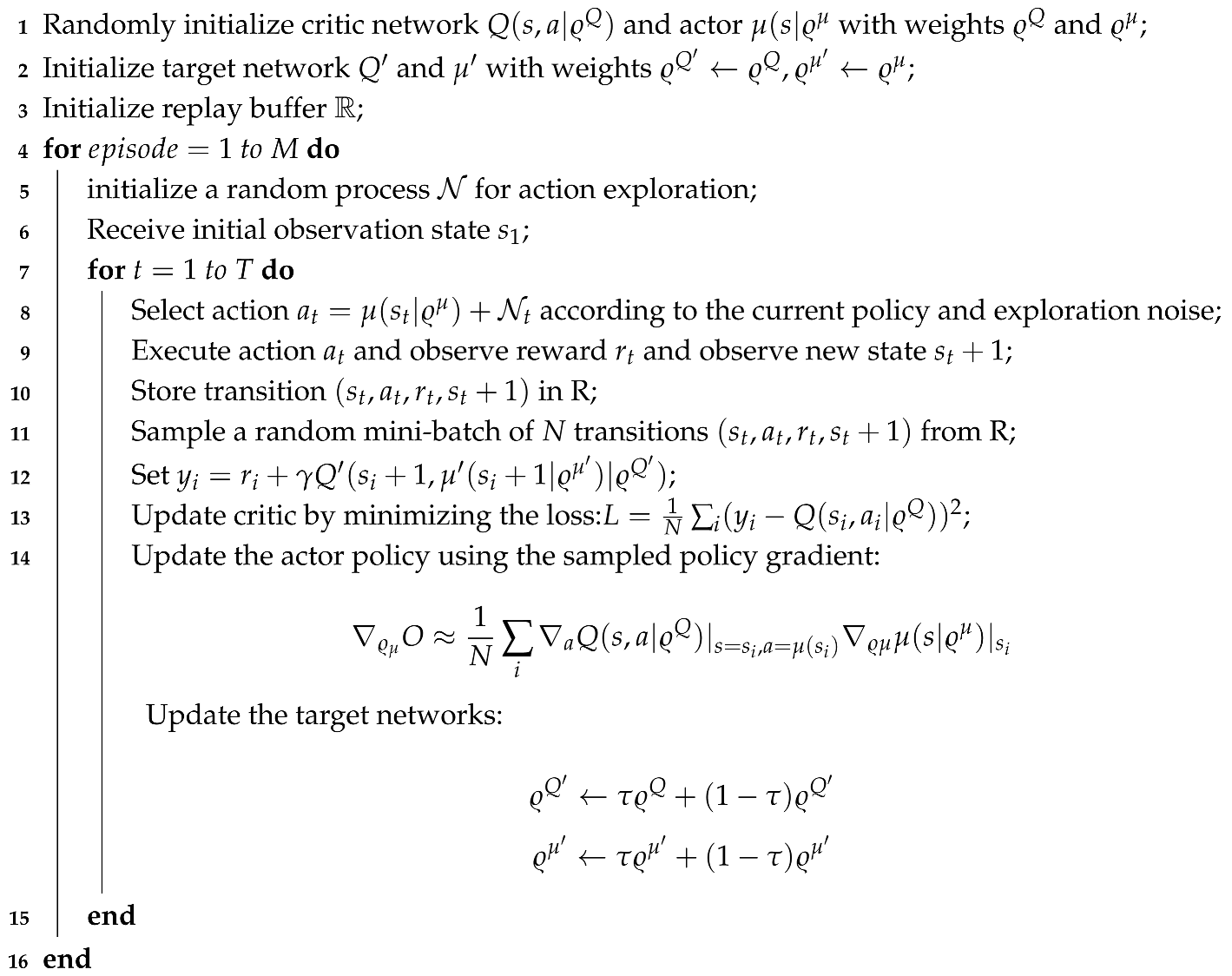4. Results And Discussions

4.1. Software Configuration

The deep reinforcement learning agent was trained using Python within a Jupyter Notebook on a Linux Ubuntu 20.04 operating system. The training process spanned approximately 5.415 hours on a modest hardware configuration consisting of an Intel graphics card, 8 GB of RAM, and a 1.9 GHz processor.

4.2. Hyper Parameter Selection and Initial Search

Parameters given in Table 2 are selected in this work.

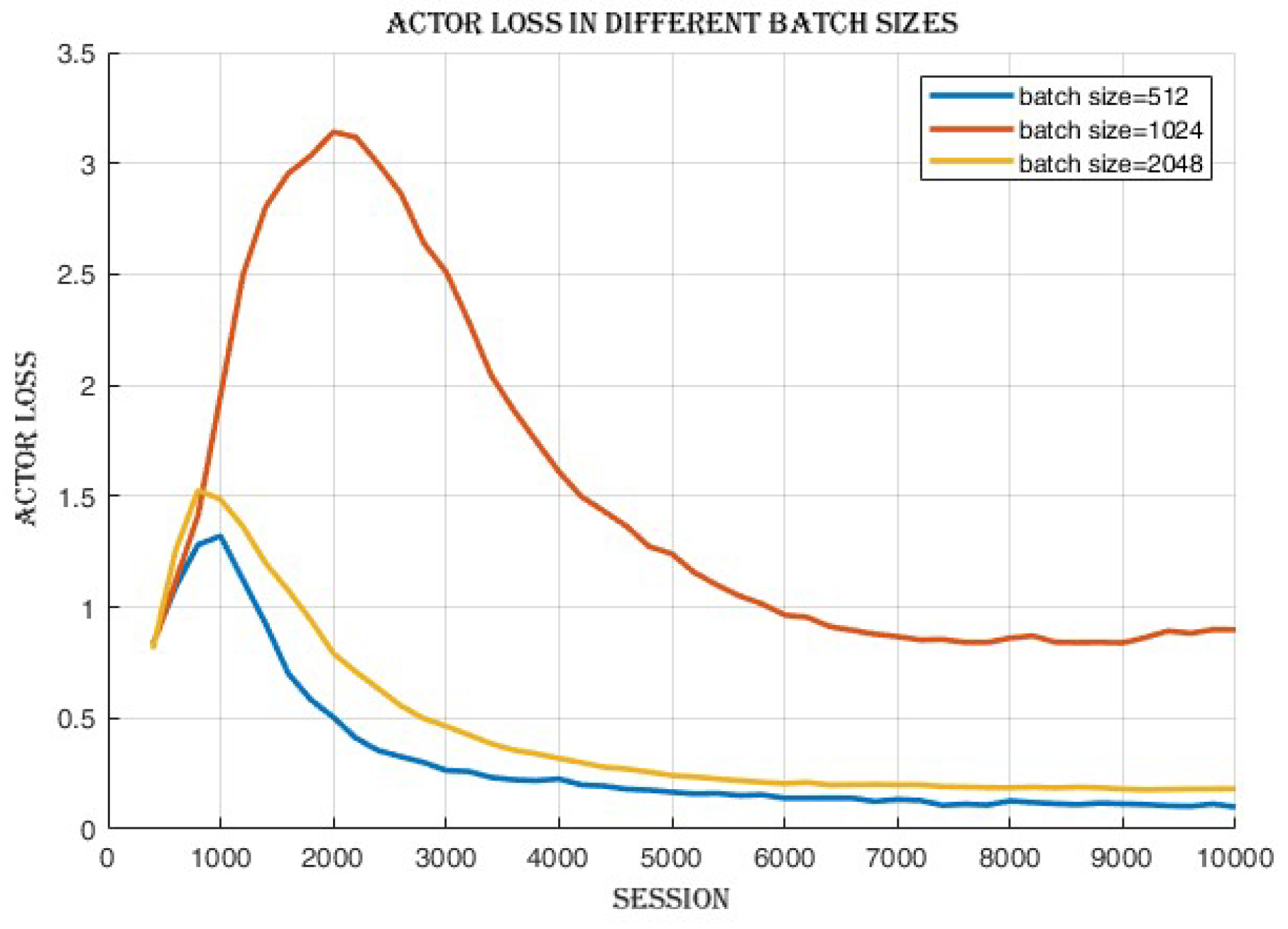
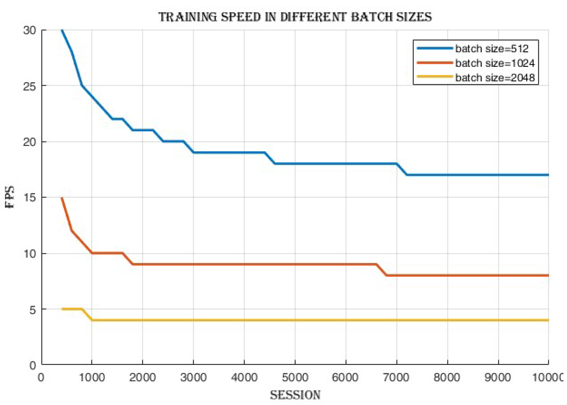
4.2.1. Batch Size Comparison

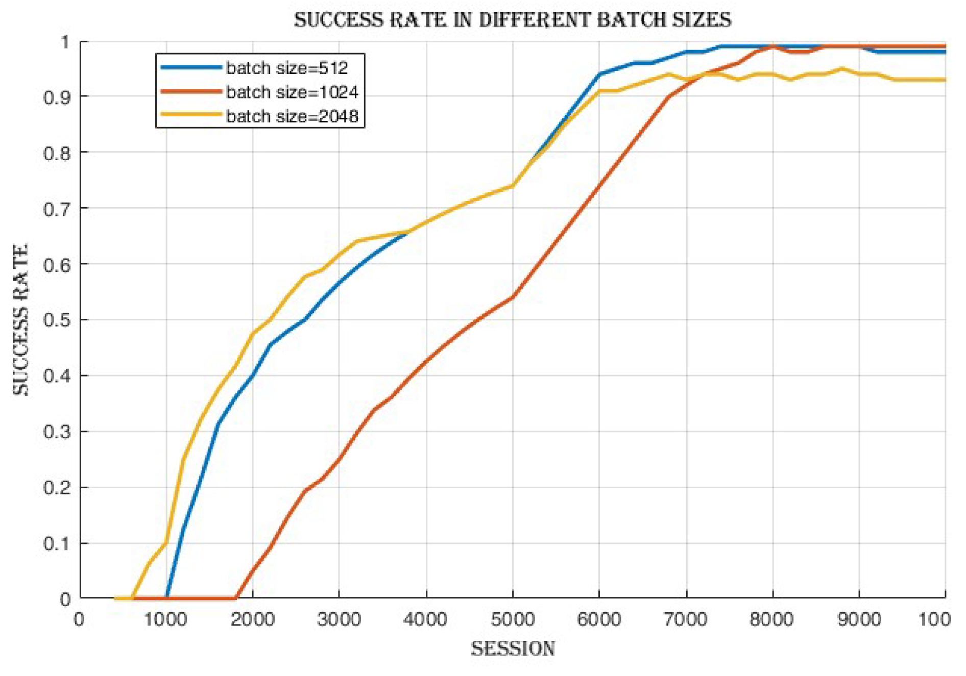
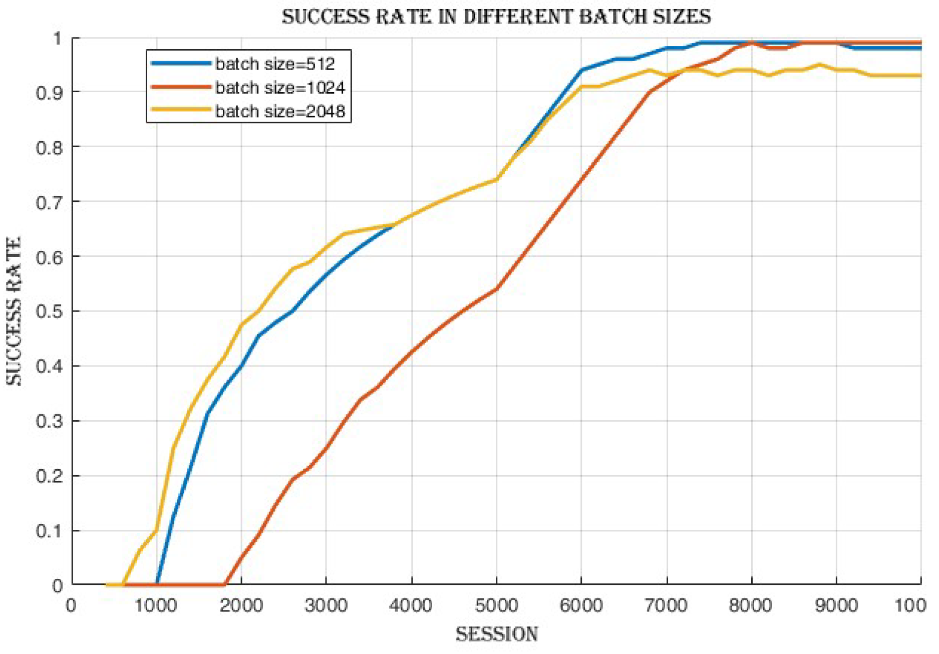
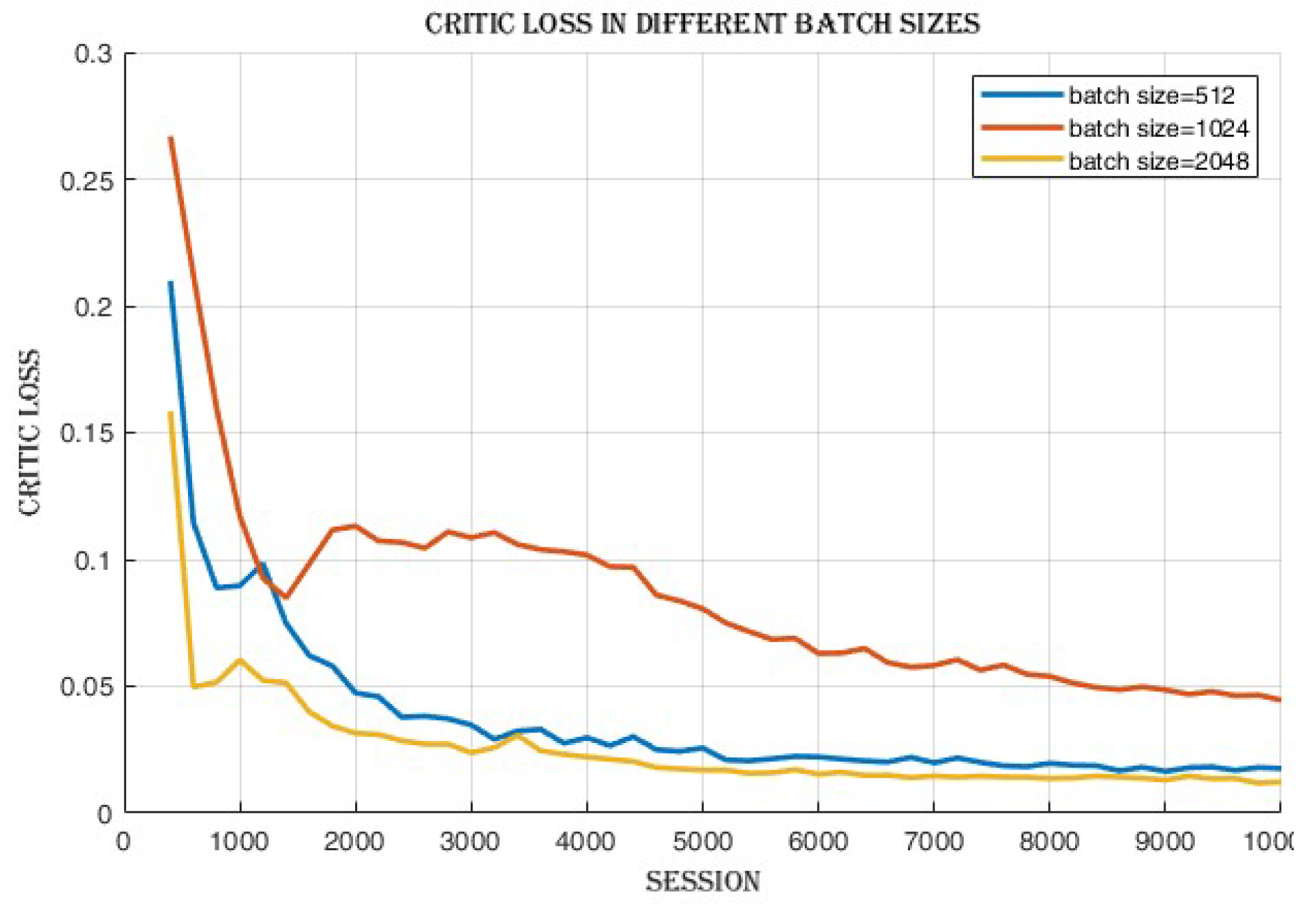
Upon completing the training process, it was observed that there was a minimal disparity in the success rate, Figure 2, and cumulative reward, Figure 3, achieved across the different batch sizes. Also, the decrease in critic loss values, Figure 4 and actor loss values, Figure 5 indicates an improvement in the actor and critic networks’ ability to approximate the optimal policy and value functions. Although the success rate and cumulative reward were similar, the enhanced convergence demonstrated by the lower losses in the 2048 batch size suggests a more efficient learning process and a potentially higher quality of learned policies.

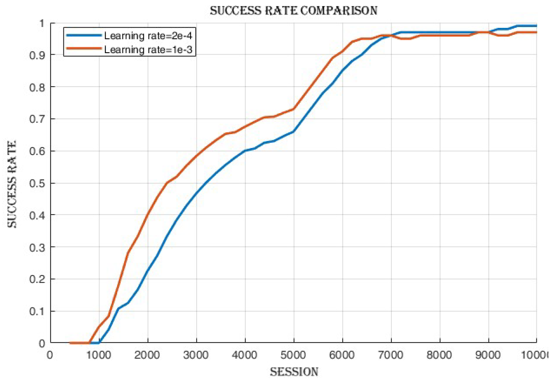
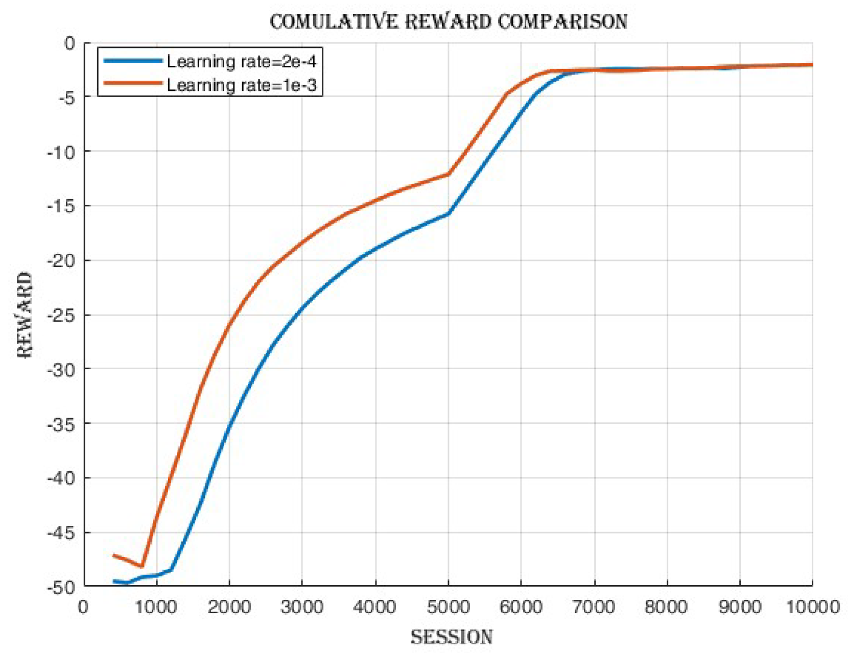
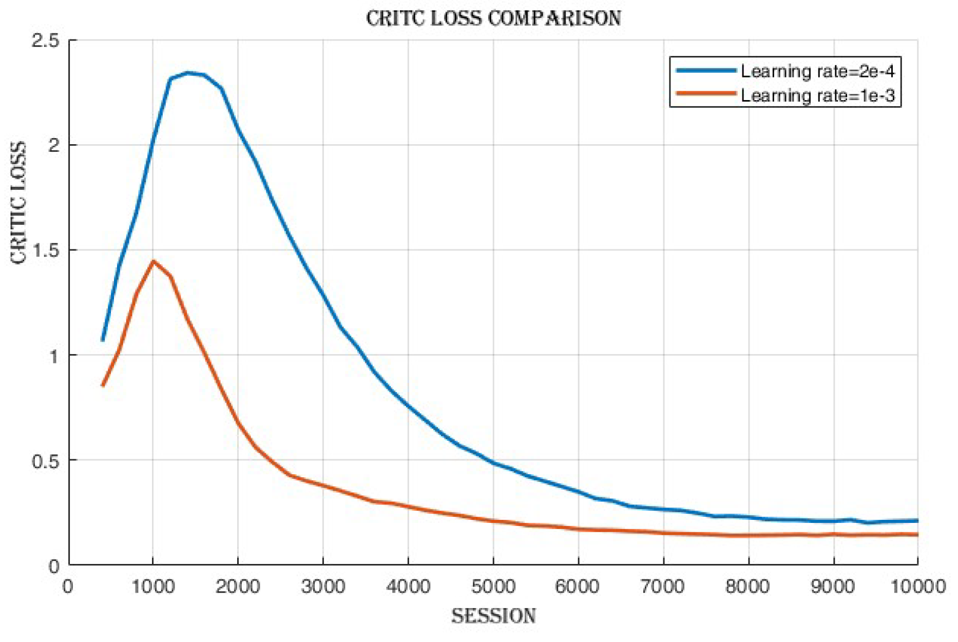
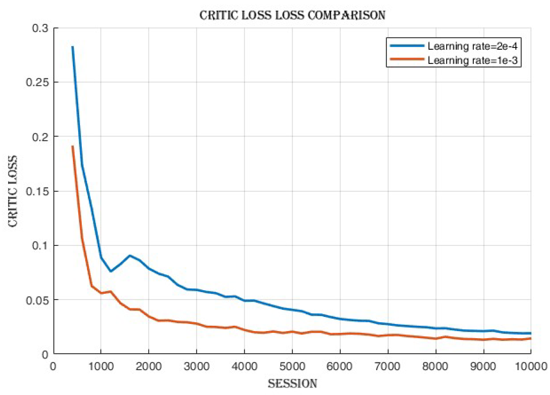
4.2.2. Learning Rate Comparison

After the training process, observations, Figure 8 revealed that there was a minimal disparity in the cumulative reward and success rate achieved between the two learning rates as shown in Figure 7. However, the learning rate of 2e-4 displayed slightly superior performance compared to 1e-3 in terms of success rate. Conversely, when using the learning rate of 1e-3, a notable decrease in actor loss, Figure 9 and critic loss, Figure 10 was observed, indicating improved policy and value estimation by the agent. Despite comparable cumulative reward and success rates, the reduced losses at the learning rate of 1e-3 signify enhanced convergence and a potentially more efficient learning process, suggesting the agent may have acquired higher-quality learned policies.

4.3. Selection of Optimal Hyperparameters and Extended Training of DDPG Agent

After comparing the hyperparameters, as depicted in the preceding figures, and conducting a thorough analysis of the associated results, the selection of hyperparameters with promising performance was undertaken. Following this, an extended training phase was initiated, encompassing 100,000 time steps. This extended training phase serves as the fundamental training stage, which will be elaborated upon in the subsequent section.

Table 3. Parameters and Selected Hyper parameters.

Parameter	Value
Policy	MultiInputPolicy
Replay buffer class	HerReplayBuffer
Verbose	1
Gamma	0.95
Tau ($\tau$)	0.005
Batch size	2048
Buffer size	100000
Replay buffer kwargs	rb kwargs
Learning rate	1e-3
Action noise	Normal action noise
Policy kwargs	Policy kwargs
Tensorboard log	Log path

Table 3. Parameters and Selected Hyper parameters.

Parameter	Value
Policy	MultiInputPolicy
Replay buffer class	HerReplayBuffer
Verbose	1
Gamma	0.95
Tau ($\tau$)	0.005
Batch size	2048
Buffer size	100000
Replay buffer kwargs	rb kwargs
Learning rate	1e-3
Action noise	Normal action noise
Policy kwargs	Policy kwargs
Tensorboard log	Log path

Table 4. Training Metrics at 200 time step and at $100,000$ time step.

Category	Value	Category	Value
rollout/		rollout/
Episode length	50	Episode length	50
Episode mean reward	-49.2	Episode mean reward	-1.8
Success rate	0	Success rate	1
time/		time/
Episodes	4	Episodes	2000
FPS	18	FPS	5
Time elapsed	10	Time elapsed	19505
Total timesteps	200	Total time steps	100000
train/		train/
Actor loss	0.625	Actor loss	0.0846
Critic loss	0.401	Critic loss	0.00486
Learning rate	0.001	Learning rate	0.001
Number of updates	50	Number of updates	99850

Table 4. Training Metrics at 200 time step and at $100,000$ time step.

Category	Value	Category	Value
rollout/		rollout/
Episode length	50	Episode length	50
Episode mean reward	-49.2	Episode mean reward	-1.8
Success rate	0	Success rate	1
time/		time/
Episodes	4	Episodes	2000
FPS	18	FPS	5
Time elapsed	10	Time elapsed	19505
Total timesteps	200	Total time steps	100000
train/		train/
Actor loss	0.625	Actor loss	0.0846
Critic loss	0.401	Critic loss	0.00486
Learning rate	0.001	Learning rate	0.001
Number of updates	50	Number of updates	99850

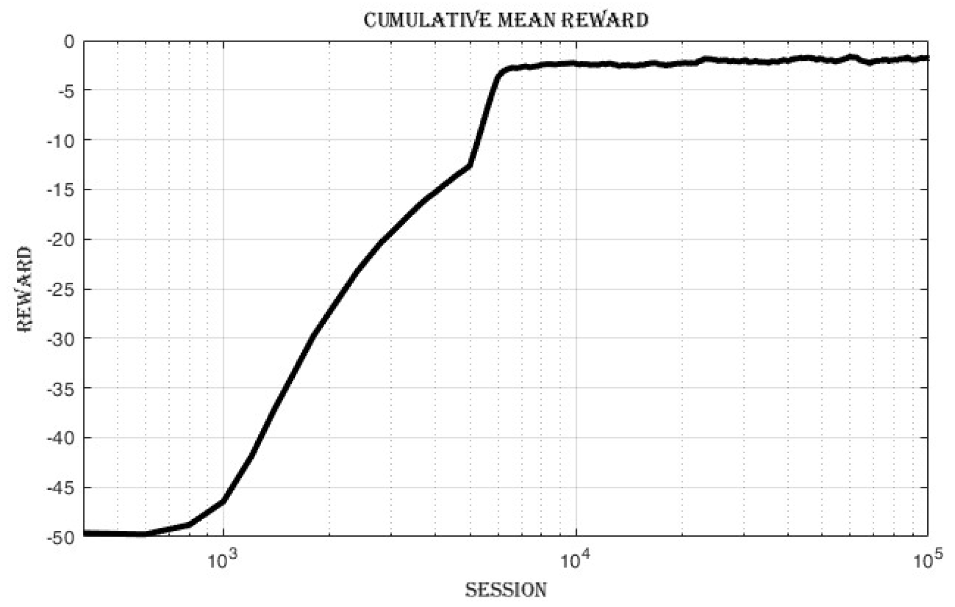
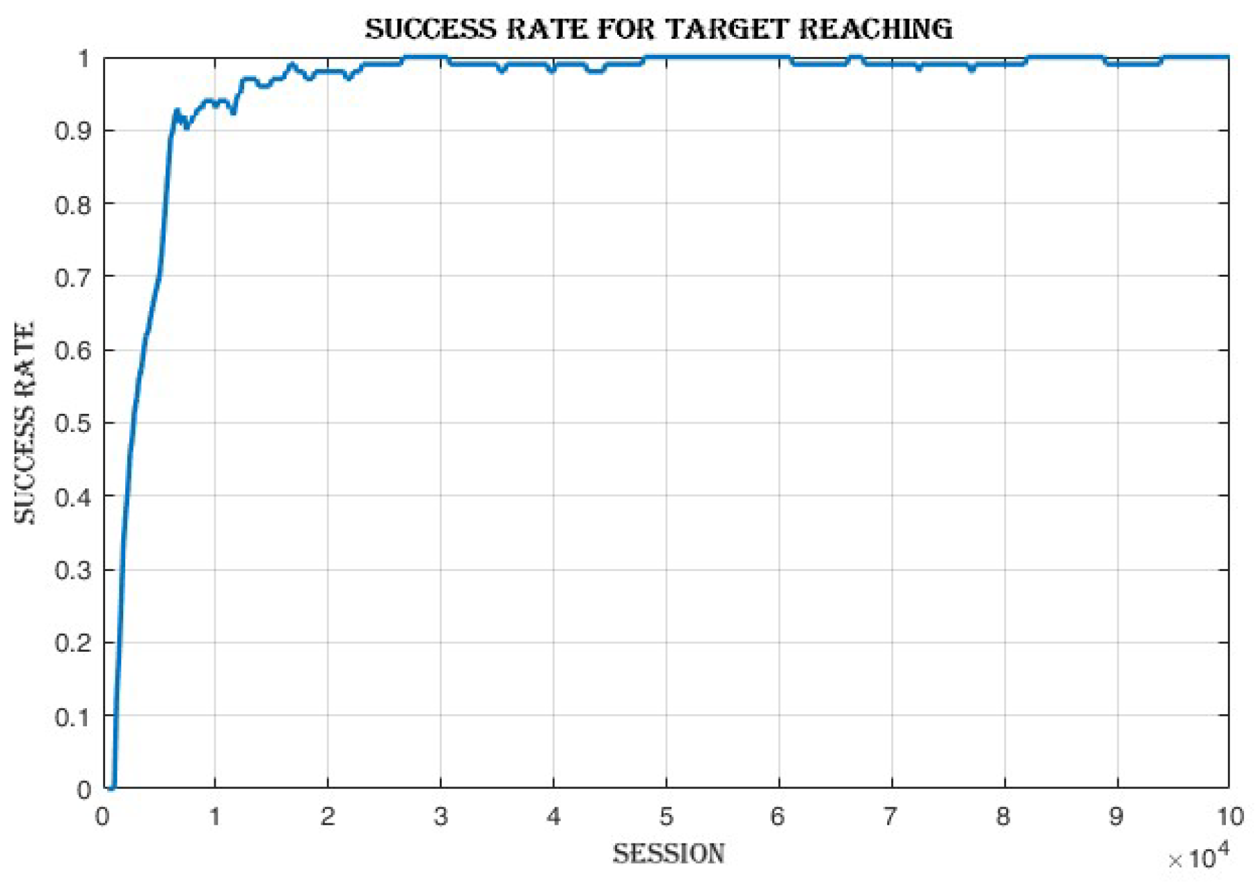
4.3.1. Improvement in Cumulative Reward and Success Rate

The mean episode reward, Figure 11 improves from -49.2 in the first loop to -1.8 in the last loop. The success rate, Figure 12 increases from 0 in the first loop to 1 in the last loop.

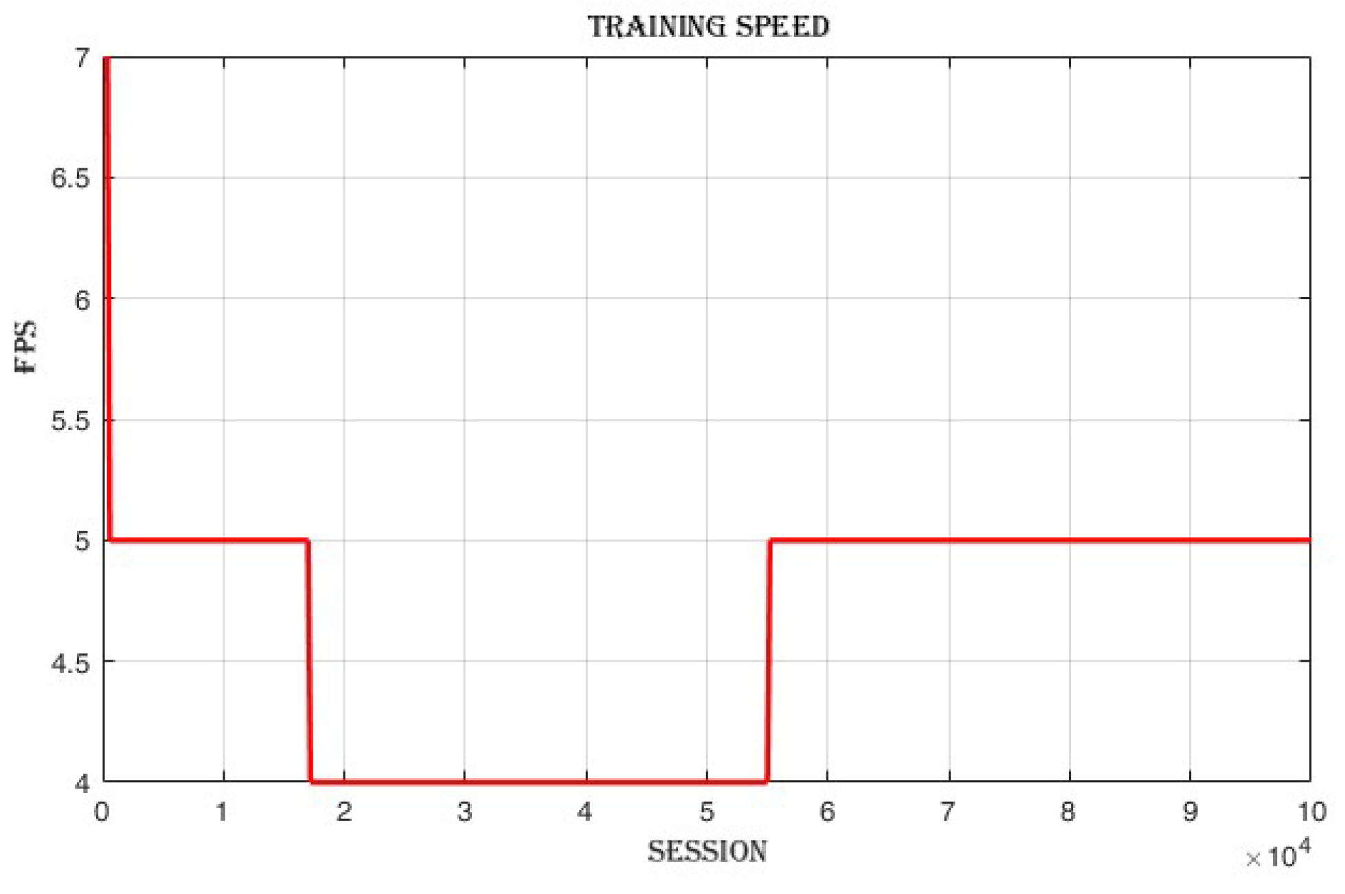
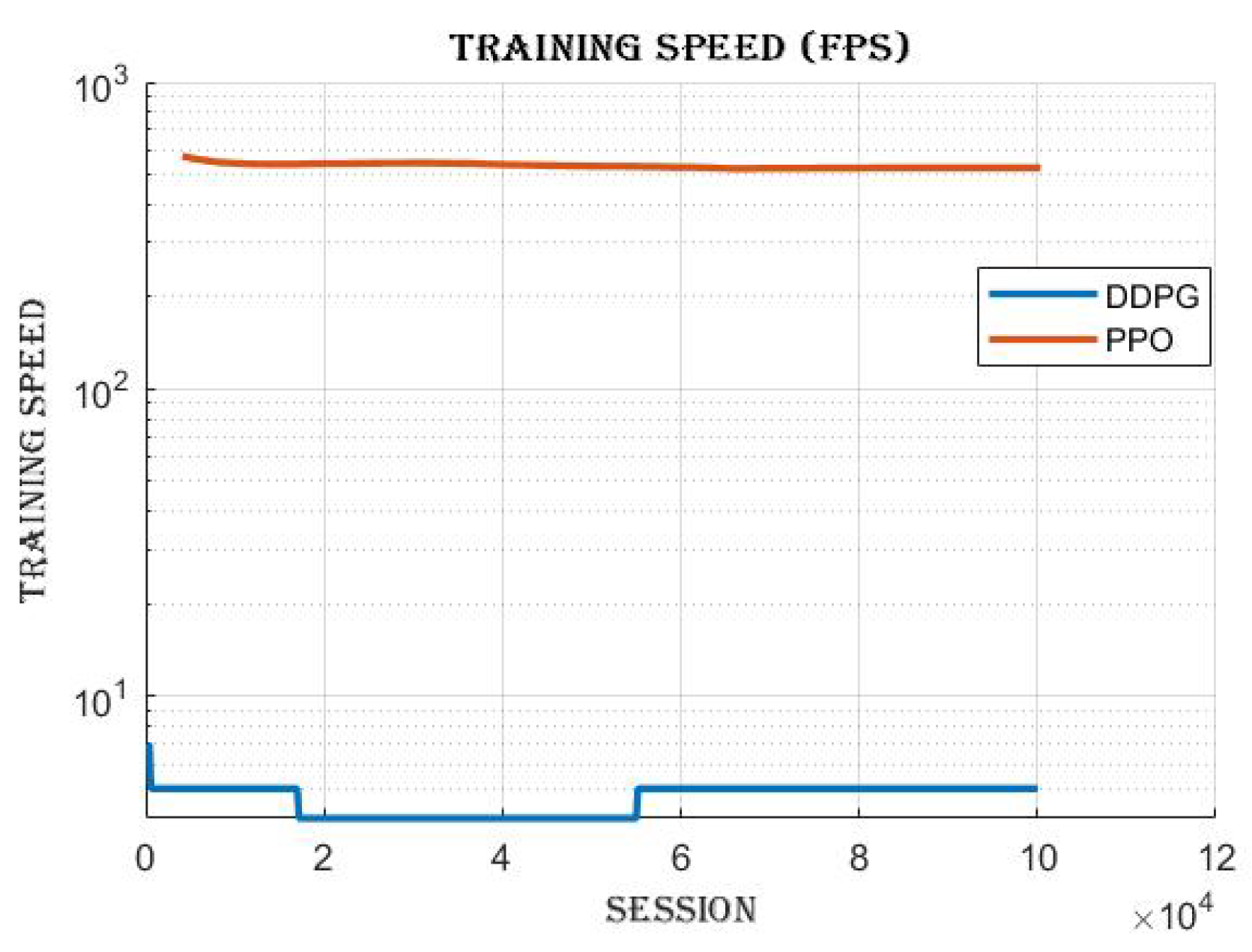
4.3.2. Frames per Second (FPS)

The training speed, Figure 13 decreases from 18 frames per second (FPS) in the first loop to 5 FPS in the last loop.

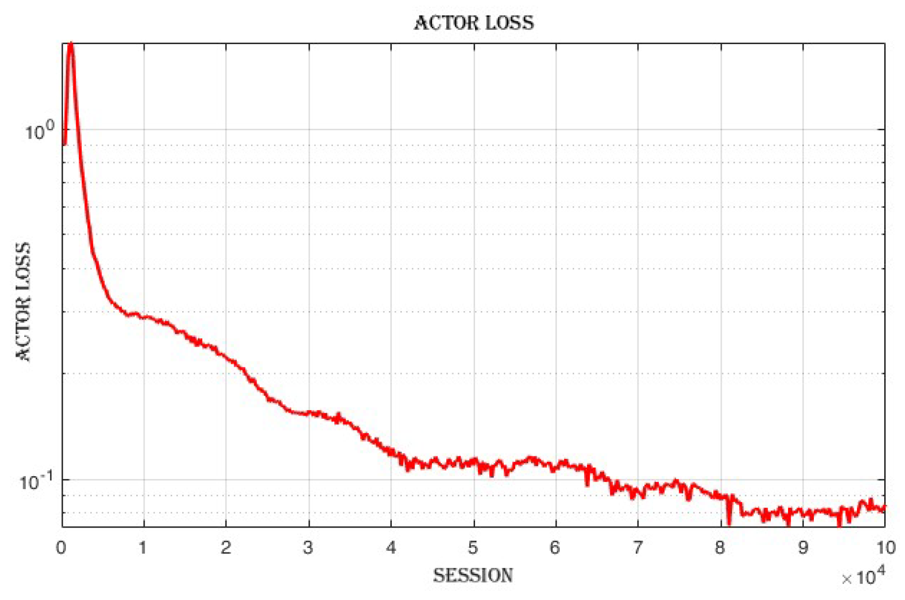
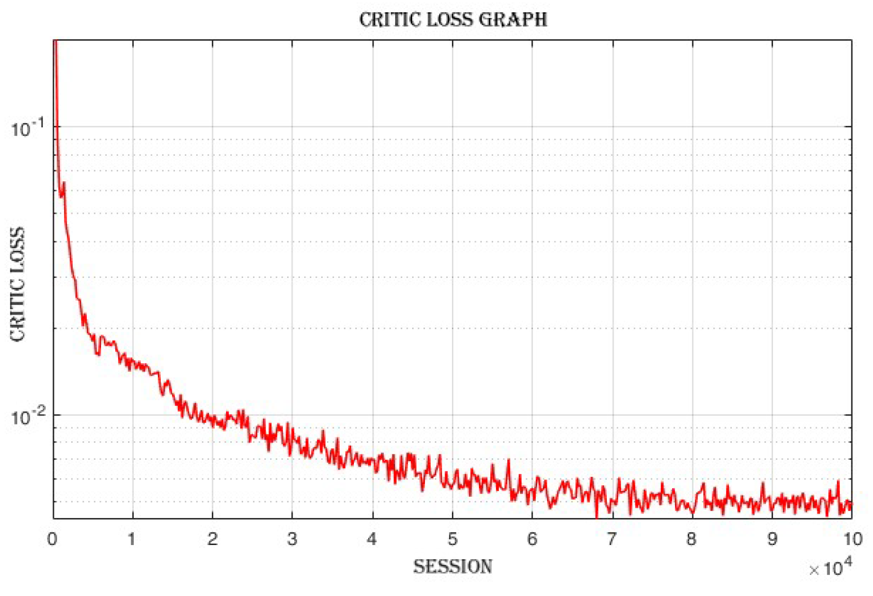
4.3.3. Improvement in Actor and Critic Losses

The actor loss, Figure 14 decreases from 0.625 in the first loop to 0.0846 in the last loop. The critic loss, Figure 15 decreases from 0.401 in the first loop to 0.00486 in the last loop.

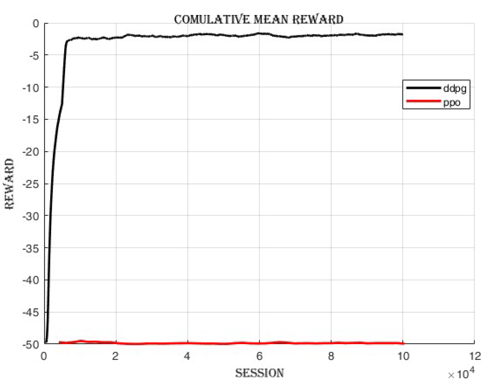
4.4. Comparing DDPG and PPO: Off-Policy vs. On-Policy Reinforcement Learning Algorithms

Proximal policy optimization (PPO), an on-policy reinforcement learning algorithm, was trained to compare its performance with Deep deterministic policy gradient (DDPG), an off-policy algorithm, as shown in Figure 16 and Figure 17. The cumulative reward achieved by DDPG was $-1.8$, whereas the cumulative reward obtained by PPO was $-50$ as shown in Figure 16. The results of this comparison indicate that, in this particular scenario, DDPG exhibited superior performance over PPO in terms of cumulative reward.

5. Conclusion

In this study, the Deep Deterministic Policy Gradient (DDPG) algorithm is applied to train a robotic arm manipulator, specifically the Franka Panda robotic arm, for a target-reaching task. The objective of this task is to enable the robotic arm to accurately reach a designated target position. The DDPG algorithm is chosen because of its effectiveness in continuous control tasks and its ability to learn policies with high-dimensional action spaces. By leveraging a combination of deep neural networks and actor-critic architecture, DDPG approximates the optimal policy for the robotic arm. When comparing the performance of PPO and DDPG after training for $100,000$ time steps:

PPO achieved a mean episode reward of $-50$ indicating that the agent struggled to achieve positive rewards on average. Despite training at a relatively fast speed of $561FPS$, the results suggest that PPO faced challenges in finding successful strategies for the given task.

On the other hand, DDPG demonstrated superior performance with a mean episode reward of $-1.8$. It achieved a success rate of 1, indicating consistent success in reaching desired outcomes. Despite a slower training speed of $5FPS$. DDPG showcased its capability to effectively learn and improve its policy over time. Based on these results, DDPG outperformed PPO in terms of cumulative reward and success rate in the given scenario.

References

- Mohsen, S.; Behrooz, A.; Roza, D. Artificial intelligence, machine learning and deep learning in advanced robotics, a review. Cognitive Robotics 2023, 3, 54–70. [Google Scholar]
- Sridharan, M.; Stone, P. Color Learning on a Mobile Robot: Towards Full Autonomy under Changing Illumination. In Proceedings of the International Joint Conference on Artificial Intelligence (IJCAI); 2007; pp. 2212–2217. [Google Scholar]
- Xinle, Y.; Minghe, Sh.; Lingling, Sh. Adaptive and intelligent control of a dual-arm space robot for target manipulation during the post-capture phase. Aerospace Science and Technology 2023, 142, 108688. [Google Scholar]
- Abayasiri, R. A. M.; Jayasekara, A. G. B. P.; Gopura, R. A. R. C.; Kazuo, K. Intelligent Object Manipulation for a Wheelchair-Mounted Robotic Arm. Journal of Robotics, 2024. [Google Scholar]
- Mohammed, M. A.; Hui, L.; Norbert, St.; Kerstin, Th. Intelligent arm manipulation system in life science labs using H20 mobile robot and Kinect sensor. 2016 IEEE 8th International Conference on Intelligent Systems (IS), Sofia, Bulgaria, 2016. [Google Scholar]
- Yoshiyuki Ohmura and Yasuo Kuniyoshi. Humanoid robot which can lift a 30kg box by whole body contact and tactile feedback. 007 IEEE/RSJ International Conference on Intelligent Robots and Systems, San Diego, CA, USA, 2007; pp. 1136–1141. [Google Scholar]
- Li, Z.; Ming, J.; Dewan, F.; Hossain, M.A. Intelligent facial emotion recognition and semantic-based topic detection for a humanoid robot. Expert Systems with Applications 2013, 40, 5160–5168. [Google Scholar]
- Martin, J. G. Muros, F. J., Maestre, J. M., and Camacho, E. F. Multi-robot task allocation clustering based on game theory. Robotics and Autonomous Systems. Robotics and Autonomous Systems 2023, 161, 104314. [Google Scholar] [CrossRef]
- Nguyen, M. N. T. Ba, D. X. A neural flexible PID controller for task-space control of robotic manipulators. Frontiers in Robotics and AI 2023, 9, 975850. [Google Scholar]
- Laurenzi, A. Antonucci, D., Tsagarakis, N. G., and Muratore, L. The XBot2 real-time middleware for robotics. Robotics and Autonomous Systems. Robotics and Autonomous Systems 2023, 163, 104379. [Google Scholar] [CrossRef]
- Zhang, L. Jiang, M., Farid, D., and Hossain, M. A. Intelligent Facial Emotion Recognition and Semantic-Based Topic Detection for a Humanoid Robot. Expert Systems with Applications 2013, 40, 5160–5168. [Google Scholar] [CrossRef]
- Floreano, D. Wood, R. J. Science, Technology, and the Future of Small Autonomous Drones. Nature 2015, 521, 460–466. [Google Scholar] [CrossRef] [PubMed]
- Chen, T. D. , Kockelman, K. M., and Hanna, J. P. Operations of a Shared, Autonomous, Electric Vehicle Fleet: Implications of Vehicle & Charging Infrastructure Decisions. Transportation Research Part A: Policy and Practice, 2016. [Google Scholar]
- Chen, Z. Jia, X., Riedel, A., and Zhang, M. A Bio-Inspired Swimming Robot. 2014 IEEE International Conference on Robotics and Automation (ICRA), 2014; pp. 2564–2564. [Google Scholar]
- Ohmura, Y. and Kuniyoshi, Y. Humanoid Robot Which Can Lift a 30kg Box by Whole Body Contact and Tactile Feedback. 2007 IEEE/RSJ International Conference on Intelligent Robots and Systems; 2007; pp. 1136–1141. [Google Scholar]
- Kappassov, Z. Corrales, J.-A., and Perdereau, V. Tactile Sensing in Dexterous Robot Hands. Robotics and Autonomous Systems 2015, 74, 195–-220. [Google Scholar] [CrossRef]
- Arisumi, H. Miossec, S., Chardonnet, J.-R., and Yokoi, K Dynamic Lifting by Whole Body Motion of Humanoid Robots. 2008 IEEE/RSJ International Conference on Intelligent Robots and Systems; 2008; pp. 668–675. [Google Scholar]
- Aryslan, M. Yevgeniy, L., Troy, H., Richard, P. A deep reinforcement-learning approach for inverse kinematics solution of a high degree of freedom robotic manipulator. Robotics 2022, 11, 44. [Google Scholar] [CrossRef]
- Serhat, O. Enver T., Erkan Z. Adaptive Cartesian space control of robotic manipulators: A concurrent learning based approach. Journal of the Franklin Institute 2024, 361, 106701. [Google Scholar]
- Kaelbling, L. P. Littman, M. L., and Moore, A. Reinforcement Learning: A Survey. Journal of Artificial Intelligence Research 1996, 4, 237–285. [Google Scholar] [CrossRef]
- Fadi, Al. , Katarina Gr. Reinforcement learning algorithms: An overview and classification. 2021 IEEE Canadian Conference on Elec-trical and Computer Engineering (CCECE); 2021; pp. 1–7. [Google Scholar]
- Thrun, S.; and Littman, M. L. Reinforcement Learning: An Introduction. AI Magazine 2000, 21, 103-. [Google Scholar]
- Smruti Amarjyoti. Deep reinforcement learning for robotic manipulation-the state of the art. arXiv:1701.08878, 2017.
- Jens, K., Bagnell. Reinforcement learning in robotics: A survey. The International Journal of Robotics Research 2013, 32, 1238–1274. [Google Scholar]
- Tianci, G. Optimizing robotic arm control using deep Q-learning and artificial neural networks through demonstration-based methodologies: A case study of dynamic and static conditions. Robotics and Autonomous Systems 2024, 104771. [Google Scholar]
- Andrea, Fr., Elisa. Robotic Arm Control and Task Training through Deep Reinforcement Learning. 2020, arXiv:2005.02632v1. [Google Scholar]
- Jonaid, Sh., Michael. Optimizing Deep Reinforcement Learning for Adaptive Robotic Arm Control. 2024, arXiv:2407.02503v1. [Google Scholar]
- Roman, P. , Jakub, K. Computation 2024, 12(6), 116. [Google Scholar]
- Wanqing, X., Yuqian. Deep reinforcement learning based proactive dynamic obstacle avoidance for safe human-robot collaboration. Manufacturing Letters 2024, 1246–1256. [Google Scholar]
- Franka Emika Documentation. Control Parameters Documentation, 2024. Available at: CrossRef.
- Weng, L. Policy Gradient Algorithms. Lil’Log, 2018. 2024. Available online: https://lilianweng.github.io/posts/2018-04-08-policy-gradient.