Submitted:
21 January 2025
Posted:
21 January 2025
Read the latest preprint version here
Abstract
Amid the advancements in computer-based chemical process modeling and simulation packages used in commercial applications aimed at accelerating chemical process design and analysis, there are still certain tasks in design optimization such as distillation column internals design that become bottlenecks due to inherent limitations in such software packages. This work demonstrated the use of soft actor-critic (SAC) reinforcement learning (RL) in automating the task of determining the optimal design of trayed multi-stage distillation column. The design environment was created using the AspenPlus® software with its RadFrac module for the required rigorous modeling of column internals. The RL computational work was achieved by developing a Python package that allows interfacing with AspenPlus®, and by implementing in OpenAI’s Gymnasium module the learning space for the state and action variables. The results evidently show that: (1) SAC RL works as automation approach for the design of distillation column internals, (2) the reward scheme in the SAC model significantly affects SAC performance, (3) column diameter is a significant constraint in achieving column internals design specification in flooding, and (4) SAC hyperparameters have varying effect on SAC performance. Therefore, SAC RL can significantly improve the design of multistage distillation column internals by automating the optimization process.
Keywords:
1. Introduction
1.1. The Challenge: Distillation Column Internals Design
1.1. The Solution: SAC algorithm-based Design Optimization
2. Methodology
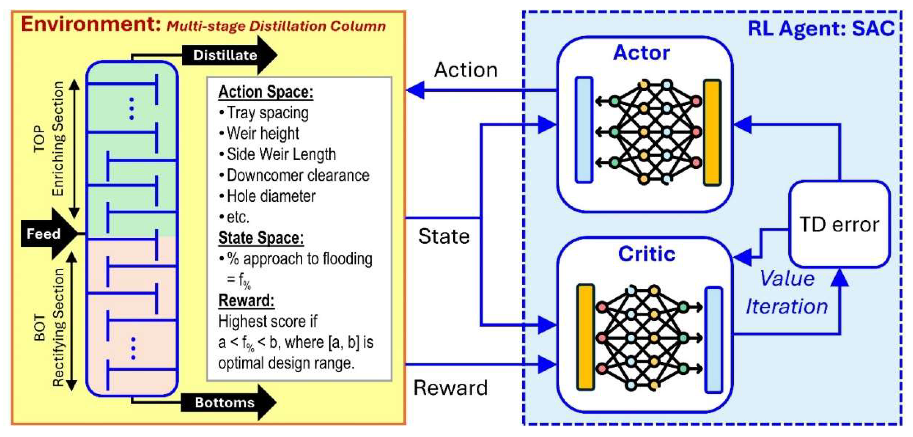
2.1 Environment: Multi-stage Distillation Column as RadFrac in AspenPlus
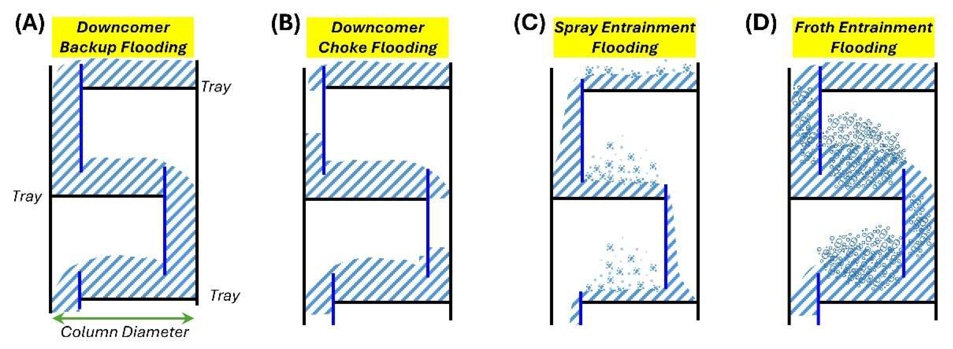
2.2 Distillation Column Flooding
2.3 Notation
2.4 SAC RL
2.5 Implementation: OpenAI Gymnasium, PyTorch
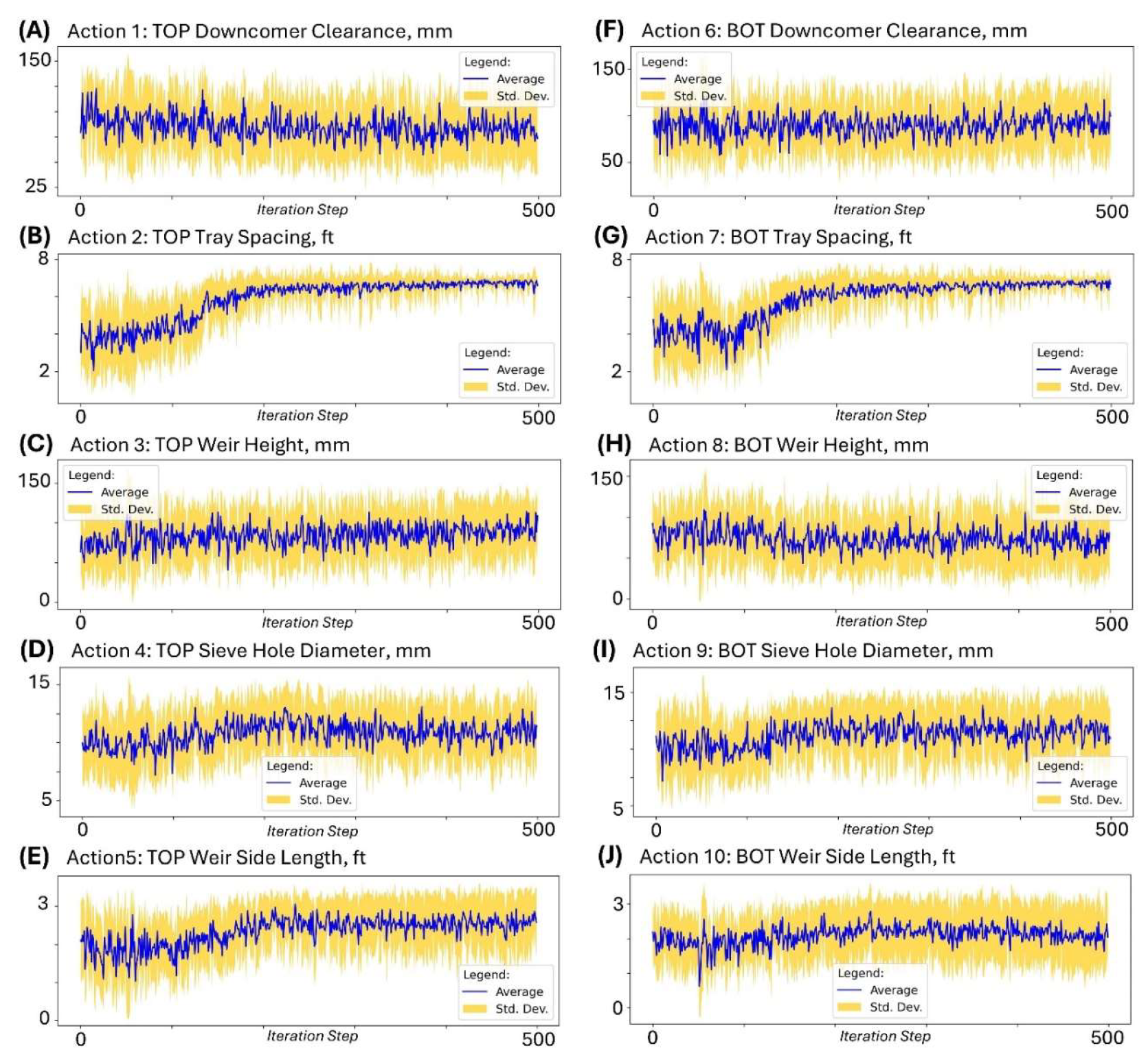
2.5.1 Action variables
2.5.2 State Variables
2.5.3 Reward Scheme
2.5.4 Hardware Setup
2.5.4 Code and Documentation of the Work Done
2.6 SAC RL Runs
2.7 Data Collection and Analysis
3. Results and Discussion
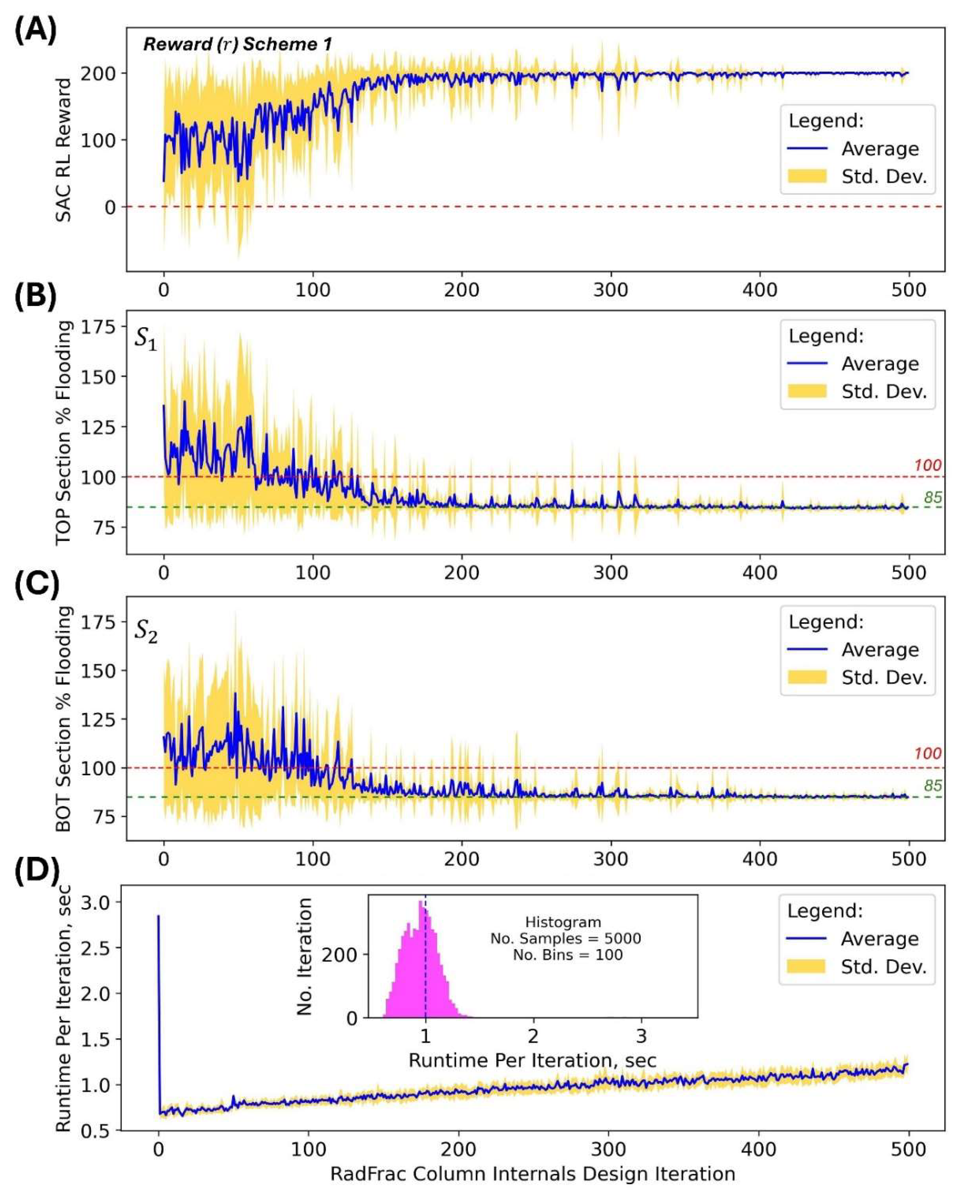
3.1 Feasibility of Using SAC RL for Distillation Column Internals Design
3.2 Effect of Reward Scheme on the Performance of SAC
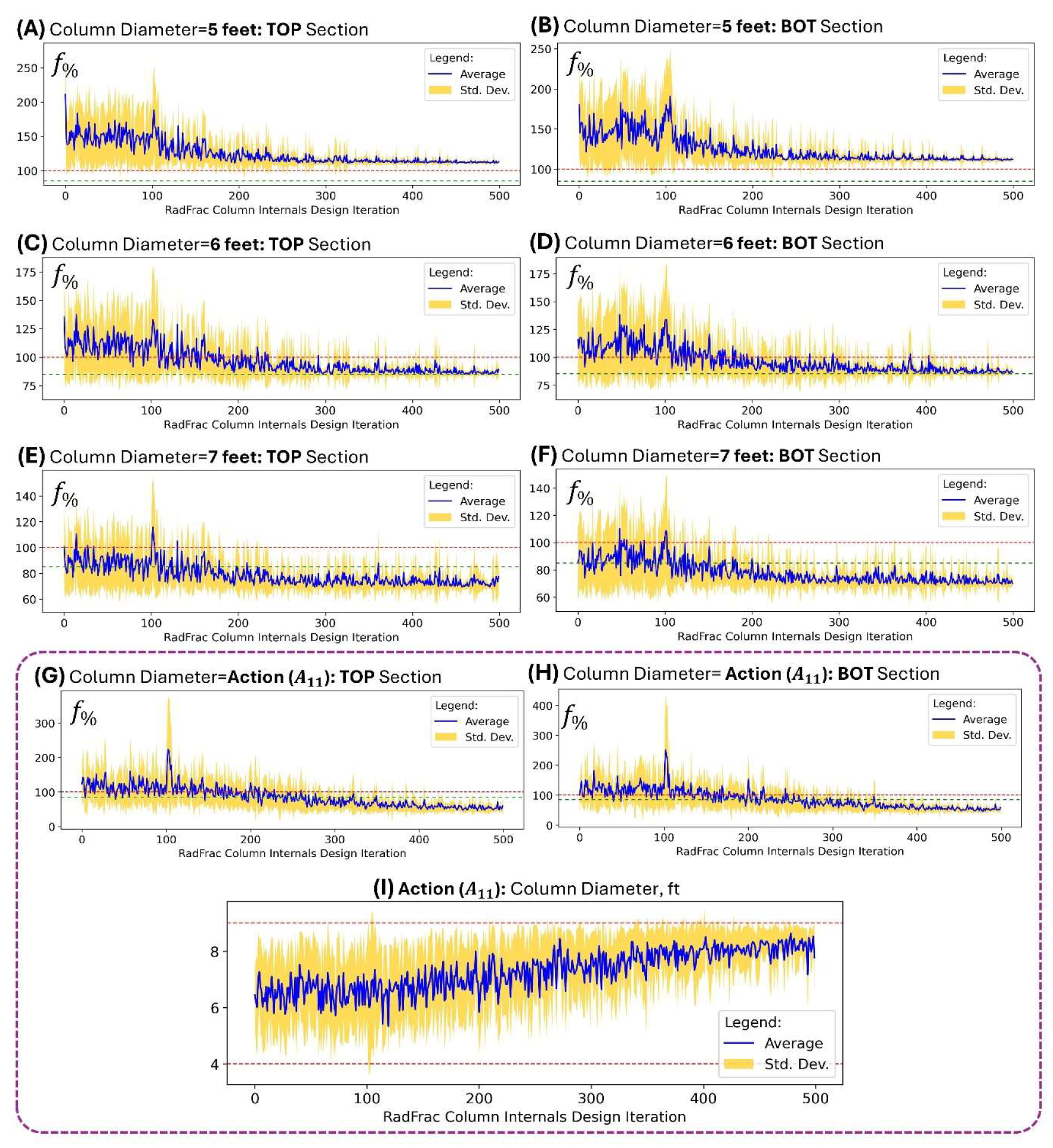
3.3 Effect of Column Diameter on the Performance of SAC
3.4 Effect of SAC Hyperparameters on Performance
4. Conclusions
Author Contributions
Funding
Data Availability Statement
Acknowledgments
Conflicts of Interest
References
- Seidel T, Biegler LT. Distillation column optimization: A formal method using stage-to stage computations and distributed streams. Chemical Engineering Science. 2025 2025/02/05/;302:120875.
- Seader JD, Henley EJ, Roper DK. Separation Process Principles: With Applications Using Process Simulators. 4th ed. New York: Wiley 2016.
- Al-Malah KIM. Aspen Plus: Chemical Engineering Applications. 2nd ed.: Wiley; 2022.
- Haydary, J. Chemical Process Design and Simulation: Aspen Plus and Aspen Hysys Applications. Wiley; 2019.
- AspenTech. AspenPlus: AspenTech; 2024 [cited v12]. Available from: https://www.aspentech.com/en.
- Bao J, Gao B, Wu X, et al. Simulation of industrial catalytic-distillation process for production of methyl tert-butyl ether by developing user’s model on Aspen plus platform. Chemical Engineering Journal. 2002 2002/12/28/;90(3):253-266.
- Kamkeng ADN, Wang M. Technical analysis of the modified Fischer-Tropsch synthesis process for direct CO2 conversion into gasoline fuel: Performance improvement via ex-situ water removal. Chemical Engineering Journal. 2023 2023/04/15/;462:142048.
- Syauqi A, Kim H, Lim H. Optimizing olefin purification: An artificial intelligence-based process-conscious PI controller tuning for double dividing wall column distillation. Chemical Engineering Journal. 2024 2024/11/15/;500:156645.
- Byun M, Lee H, Choe C, et al. Machine learning based predictive model for methanol steam reforming with technical, environmental, and economic perspectives. Chemical Engineering Journal. 2021 2021/12/15/;426:131639.
- Schefflan, R. Teach Yourself the Basics of Aspen Plus. 2nd ed.: Wiley; 2016.
- Agarwal RK, Shao Y. Process Simulations and Techno-Economic Analysis with Aspen Plus. In: Agarwal RK, Shao Y, editors. Modeling and Simulation of Fluidized Bed Reactors for Chemical Looping Combustion. Cham: Springer International Publishing; 2024. p. 17-73.
- Chen Q, editor The Application of Process Simulation Software of Aspen Plus Chemical Engineering in the Design of Distillation Column. Cyber Security Intelligence and Analytics; 2020 2020//; Cham: Springer International Publishing.
- Haarnoja T, Zhou A, Abbeel P, et al. Soft Actor-Critic: Off-Policy Maximum Entropy Deep Reinforcement Learning with a Stochastic Actor. arXiv e-prints. 2018. arXiv:1801.01290.
- Haarnoja T, Zhou A, Hartikainen K, et al. Soft Actor-Critic Algorithms and Applications. ArXiv. 2018;abs/1812.05905.
- Wankat, P. Separation Process Engineering - Includes Mass Transfer Analysis. 3rd ed. New York: Prentice Hall; 2012. (Wankat P, editor.).
- Kister, H. Distillation Design. Boston: McGraw-Hill; 1992.
- Taqvi SA, Tufa LD, Muhadizir S. Optimization and Dynamics of Distillation Column Using Aspen Plus®. Procedia Engineering. 2016 2016/01/01/;148:978-984.
- Tapia JFD. Chapter 16 - Basics of process simulation with Aspen Plus∗. In: Foo DCY, editor. Chemical Engineering Process Simulation (Second Edition): Elsevier; 2023. p. 343-360.
- Hammond, M. pywin32: PyPi; 2024 [cited 2025 Jan. 9]. Available from: https://pypi.org/project/pywin32/.
- OpenAI. Soft Actor-Critic: OpenAI; 2025 [cited 2025 Jan. 9]. Available from: https://spinningup.openai.com/en/latest/algorithms/sac.html.
- McCabe WL, Thiele EW. Graphical Design of Fractionating Columns. Industrial & Engineering Chemistry. 1925 1925/06/01;17(6):605-611.
- Jones E, Mellborn M. Fractionating column economics. Chemical Engineering Progress (CEP). 1982:52-55.
- Lillicrap TP, Hunt JJ, Pritzel A, et al. Continuous control with deep reinforcement learning. arXiv e-prints. 2015. arXiv:1509.02971.
- Towers M, Kwiatkowski A, Terry J, et al. Gymnasium: A Standard Interface for Reinforcement Learning Environments. arXiv e-prints. 2024. arXiv:2407.17032.
- Brockman G, Cheung V, Pettersson L, et al. OpenAI Gym. ArXiv. 2016;abs/1606.01540.
- Zhang X, Mao W, Mowlavi S, et al. Controlgym: Large-Scale Control Environments for Benchmarking Reinforcement Learning Algorithms. arXiv e-prints. 2023. arXiv:2311.18736.
- Nath A, Oveisi A, Pal AK, et al. Exploring reward shaping in discrete and continuous action spaces: A deep reinforcement learning study on Turtlebot3. PAMM. 2024 2024/10/01;24(3):e202400169.
- Viswanadhapalli JK, Elumalai VK, S S, et al. Deep reinforcement learning with reward shaping for tracking control and vibration suppression of flexible link manipulator. Applied Soft Computing. 2024 2024/02/01/;152:110756.
- Veviurko G, Böhmer W, de Weerdt M. To the Max: Reinventing Reward in Reinforcement Learning. arXiv e-prints. 2024. arXiv:2402.01361.
- Dayal A, Cenkeramaddi LR, Jha A. Reward criteria impact on the performance of reinforcement learning agent for autonomous navigation. Applied Soft Computing. 2022 2022/09/01/;126:109241.
- Anaconda. Anaconda: The Operating System for AI: Anaconda; 2025. Available from: https://www.anaconda.com/.
- Liu J, Guo Q, Zhang J, et al. Perspectives on Soft Actor–Critic (SAC)-Aided Operational Control Strategies for Modern Power Systems with Growing Stochastics and Dynamics. Applied Sciences. 2025 [cited. [CrossRef]
- Fortela DLB. aspenRL: Enhanced AspenPlus-based Multi-stage Distillation Design Using SAC Reinforcement Learning: GitHub; 2025 [cited 2025 Jan. 19]. Available from: https://github.com/dhanfort/aspenRL.
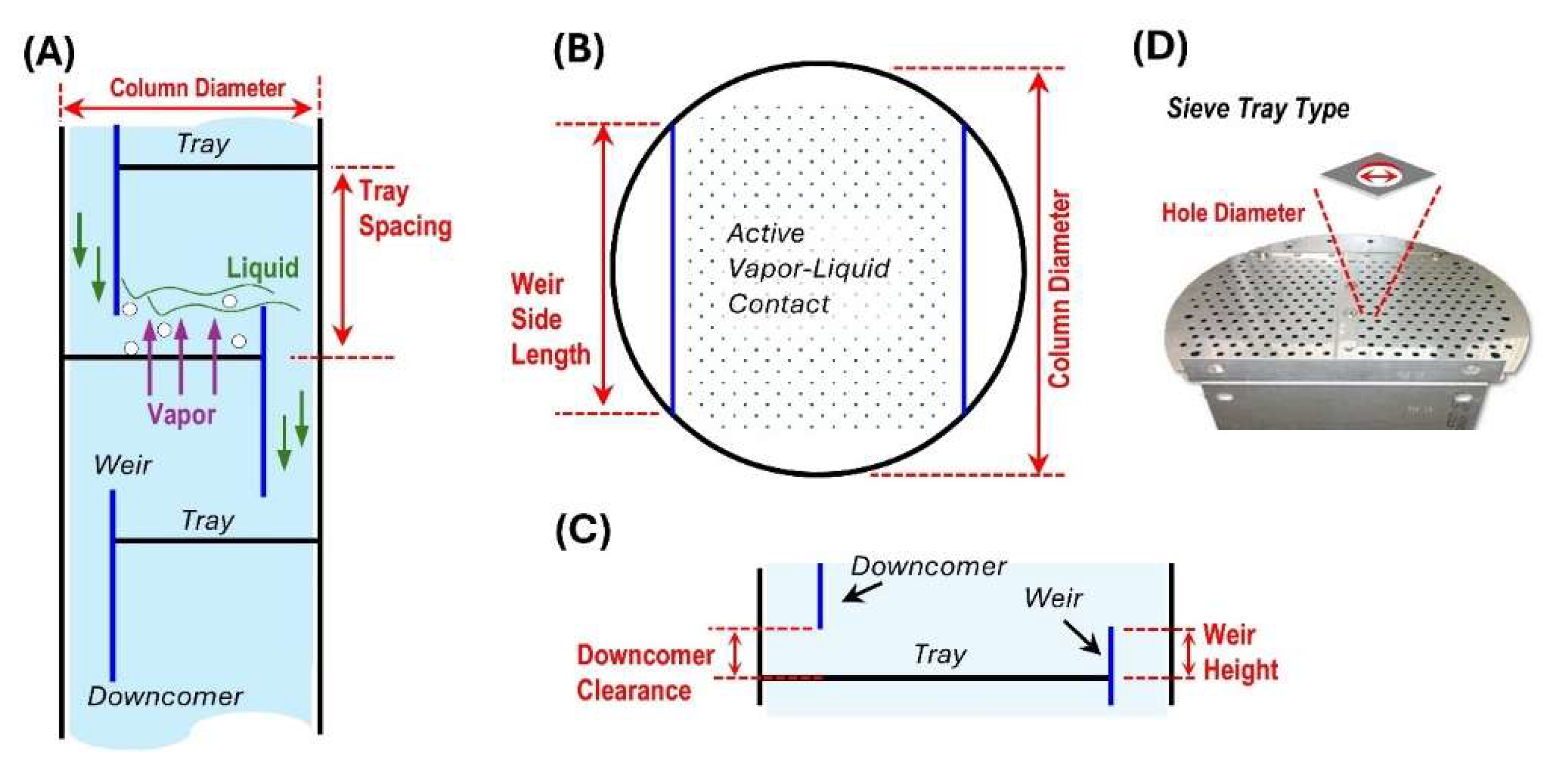

| Action/State Variable | Description |
| ) = TOP Downcomer clearance | Distance between the bottom edge of the downcomer and the tray below; Value range: [30, 150]; Units: mm |
| ) = TOP Tray spacing | Distance between two consecutive trays; Value range: [1, 7]; Units: ft |
| ) = TOP Weir height | Height of a tray outlet weir, which regulates the amount of liquid build-up on the plate surface; Value range: [10, 150]; Units: mm |
| ) = TOP Sieve hole diameter | Diameter of the holes on the sieve tray; Value range: [5, 15]; Units: mm |
| ) = TOP Weir side length | Length of the tray outlet weir; Value range: [0.1, 1]; Units: ft |
| ) = BOT Downcomer clearance | Distance between the bottom edge of the downcomer and the tray below; Value range: [30, 150]; Units: mm |
| ) = BOT Tray spacing | Distance between two consecutive trays; Value range: [1, 7]; Units: ft |
| ) = BOT Weir height | Height of a tray outlet weir, which regulates the amount of liquid build-up on the plate surface; Value range: [10, 150]; Units: mm |
| ) = BOT Sieve hole diameter | Diameter of the holes on the sieve tray; Value range: [5, 15]; Units: mm |
| ) = BOT Weir side length | Length of the tray outlet weir; Value range: [0.1, 1]; Units: ft |
| ) = Column diameter** | Diameter of the column; Value range: [4, 9]; Units: ft |
| ; Units: % | |
| ; Units: % |
| Reward Model | Definition |
| Scheme 1 |
where is the reward in section of the column. For each : where or |
| Scheme 2 |
where is the reward in section of the column. For each : where |
| Scheme 3 | Reward is based on the intervals of with highest score for the target interval . where is the reward in section of the column. For each : if ; if ; if ; if ; if ; if ; if ; if ; if ; if ; if ; if ; if |
| Scheme 4 | Reward is similar to Scheme 3 but with reward values lower by a factor of 10. where is the reward in section of the column. For each : if ; if ; if ; if ; if ; if ; if ; if ; if ; if ; if ; if ; if |
| Scheme 5 |
where is the reward in section of the column. For each : |
| Reward Model | Column Section | ||||||
| Scheme 1 | TOP | 88.5 | 8.7 | 0.955 | 0.826 | 0.251 | 0 |
| BOT | 88.8 | 8.6 | 0.945 | 0.796 | 0.216 | 0 | |
| Scheme 2 | TOP | 87.9 | 7.1 | 0.963 | 0.837 | 0.293 | 0 |
| BOT | 88.2 | 6.1 | 0.974 | 0.835 | 0.146 | 0 | |
| Scheme 3 | TOP | 87.7 | 6.0 | 0.971 | 0.841 | 0.29 | 0 |
| BOT | 88.0 | 5.6 | 0.976 | 0.823 | 0.214 | 0 | |
| Scheme 4 | TOP | 93.8 | 14.6 | 0.851 | 0.587 | 0.111 | 0 |
| BOT | 94.0 | 14.6 | 0.845 | 0.57 | 0.102 | 0 | |
| Scheme 5 | TOP | 101.9 | 21.8 | 0.686 | 0.371 | 0.067 | 0 |
| BOT | 102.4 | 22.0 | 0.686 | 0.359 | 0.052 | 0 |
| SAC Setting | Hyperparameter | Fraction of | Mean | Std. Dev. | |||
| Replay buffer length | |||||||
| 1 | 0.2 | 0.05 | 0.99 | 50 | 0.945 | 85.3 | 4.0 |
| 2 | 0.2 | 0.05 | 0.9 | 50 | 0.918 | 85.9 | 3.6 |
| 3 | 0.5 | 0.05 | 0.9 | 100 | 0.881 | 86.8 | 5.3 |
| 4 | 0.2 | 0.05 | 0.9 | 100 | 0.886 | 86.8 | 6.3 |
| 5 | 0.2 | 0.05 | 0.99 | 100 | 0.826 | 88.5 | 8.7 |
| 6 | 0.2 | 0.01 | 0.99 | 50 | 0.978 | 84.8 | 2.1 |
| 7 | 0.5 | 0.01 | 0.9 | 50 | 0.865 | 86.8 | 5.2 |
| 8 | 0.1 | 0.01 | 0.9 | 50 | 0.881 | 86.7 | 5.1 |
| 9 | 0.2 | 0.01 | 0.9 | 50 | 0.938 | 85.4 | 3.2 |
| 10 | 0.5 | 0.01 | 0.9 | 100 | 0.916 | 86.5 | 5.3 |
| 11 | 0.1 | 0.01 | 0.9 | 100 | 0.947 | 85.8 | 3.2 |
| 12 | 0.2 | 0.01 | 0.9 | 100 | 0.932 | 86.4 | 6.1 |
| 13 | 0.2 | 0.01 | 0.99 | 100 | 0.870 | 87.5 | 7.7 |
Disclaimer/Publisher’s Note: The statements, opinions and data contained in all publications are solely those of the individual author(s) and contributor(s) and not of MDPI and/or the editor(s). MDPI and/or the editor(s) disclaim responsibility for any injury to people or property resulting from any ideas, methods, instructions or products referred to in the content. |
© 2025 by the authors. Licensee MDPI, Basel, Switzerland. This article is an open access article distributed under the terms and conditions of the Creative Commons Attribution (CC BY) license (http://creativecommons.org/licenses/by/4.0/).


