
Submitted:
20 January 2025
Posted:
20 January 2025
You are already at the latest version
Abstract
This study analyzes a system of interacting particles influenced by gravitational forces and internal Lennard-Jones interactions, focusing on energy redistribution and introducing D-Entropy as a measure of internal energy changes. Numerical simulations reveal that, despite overall energy conservation, significant initial fluctuations in individual energy components occur due to complex interactions. The system shows dynamic energy redistribution, particularly as it transitions from a far-from-equilibrium state to a stable configuration, with D-Entropy capturing periods of rapid energy exchange followed by reduced fluctuations.Particle trajectories exhibit complex behaviors, including deviations and oscillations driven by gravitational and Lennard-Jones forces. Nonlinear interactions significantly impact energy redistribution and system stability. The results demonstrate the utility of D-Entropy in quantifying energy changes and provide insights into the thermodynamic evolution of structured bodies.Future research will incorporate dissipative forces, explore other interaction potentials, and scale up the system to study collective effects and phase transitions. These findings have potential applications in materials science, astrophysics, and other fields involving dynamic structured systems.
Keywords:
Entropy
; energy
; evolution
; nonlinearity
; determinism
; probability
1. Introduction
Motion and fundamental interactions are inherent properties of matter, but evolution should also be considered as a fundamental aspect. Evolution is not merely a combination of motion and interactions; it encompasses the processes of birth, development, and decay of complex systems. While well-developed theories exist for studying the dynamics and interactions of matter, comprehensive theories that describe evolutionary processes are still lacking [1].
As Ilya Prigogine noted, we currently have a physics of “the existing,” but we lack a “physics of the emerging,” which we will refer to as the “physics of evolution” [1]. The main objective of this field is to describe the processes of formation, development, and decay of systems within the framework of fundamental physical laws. Achieving this goal requires accounting for all processes that occur during the motion of objects in non-uniform external force fields. This is particularly important for studying the evolution of the universe, where such processes cannot be ignored [2,3].
However, the path to creating a physics of evolution is fraught with challenges. One of the main problems is the lack of unity in modern physics: it is divided into several fragments, each dealing with separate aspects of nature—such as mechanics and thermodynamics—but insufficiently describing their interactions [2]. To effectively describe evolution, it is necessary to connect these fragments, creating a unified theory that considers not only the dynamics of objects but also their internal states.
Today, physics is conventionally divided into two sections. The first section includes disciplines that study the dynamics and interactions of objects based on fundamental physical laws, such as Newton’s laws [4,5,6]. However, the role of a body’s internal structure in its motion is not taken into account, limiting the ability to describe processes related to changes in internal energy, such as dissipation.
The second section addresses the behavior of internal states of bodies in response to changes in external conditions. Here, models often represent large closed systems that can be described using statistical ensembles of equilibrium subsystems. This approach allows the use of statistical physics methods to study processes occurring in these systems and considers entropy as a measure of disorder [7].
Yet, a problem remains: classical mechanics describes processes as reversible, whereas thermodynamic processes are irreversible. To resolve this contradiction, attempts have been made to introduce a dynamic interpretation of entropy using positive Lyapunov exponents, which determine the nature of system mixing. However, such methods rely on probabilistic laws and therefore cannot be used to construct a complete deterministic theory [7].
In this work, the concept of D-entropy is introduced, defining changes in the internal energy of a system moving in non-uniform external force fields. D-entropy is characterized as the ratio of the change in internal energy to its total magnitude, allowing for the consideration of energy redistribution between the ordered and chaotic components of motion. D-entropy not only links the dynamics of bodies with thermodynamics but also resolves contradictions between them, opening up the possibility of creating a physics of evolution that describes processes of formation, development, and decay of systems within the framework of physical laws [7,8].
Thus, D-entropy becomes an important tool for analyzing evolutionary processes. It is applicable in both mechanics and thermodynamics and allows for determining how the internal state of a system changes under the influence of external forces. This is crucial for understanding dissipation processes and the transition to thermodynamic equilibrium.
2. Theoretical Background
2.1. Concept of Structured Bodies
In classical mechanics, the concept of a material point is often used to simplify the analysis of motion. A material point is an idealized object, which has mass but no internal structure or spatial extent. It allows us to focus on the translational motion without considering any internal dynamics or deformation.
However, real physical objects often have an internal structure that plays a significant role in their dynamics, especially in the presence of external forces or interactions between particles. These objects are referred to as structured bodies. A structured body is characterized not only by its mass and position but also by its internal state, which may involve factors like deformation, relative motions of constituent particles, and internal stresses.
The key difference between a structured body and a material point lies in the consideration of internal degrees of freedom:
- A material point is described by a limited number of degrees of freedom, typically three for translational motion in space.
- A structured body, on the other hand, has additional degrees of freedom that account for internal dynamics. This includes relative motion between different parts of the body, rotational dynamics, and deformations that result from external forces [9].
2.2. Difference Between Structured Bodies and Material Points
The main differences between structured bodies and material points can be summarized as follows:
- 1)
- Degrees of Freedom: A material point has only translational degrees of freedom, whereas a structured body has additional internal degrees of freedom, such as rotation, deformation, and internal vibration.
- 2)
- Energy Representation: For a material point, the energy is solely associated with its translational motion. For a structured body, the energy also includes internal kinetic and potential energy due to the interactions and relative motion of its constituent particles.
- 3)
- Interaction with External Fields: Structured bodies have a more complex response to external fields due to their internal structure. Internal forces and energy redistribution play a significant role in determining the body’s behavior under external influences.
The difference between structured bodies and material points is crucial for understanding the limitations of classical mechanics when applied to real physical systems:
- Material Points: Only possess translational degrees of freedom, and their energy is associated solely with the motion of the center of mass.
- Structured Bodies: Possess additional degrees of freedom that account for internal interactions, rotations, deformations, and relative motions. These internal dynamics result in complex energy exchanges that cannot be captured by treating the system as a simple material point.
2.3. Equation of Motion for a Structured Body
To describe the dynamics of a structured body, it is essential to account for both the macroscopic motion of the body as a whole and the microscopic motions of its internal constituents. The equation of motion for a structured body can be derived by applying Newton’s second law to both the center of mass and the internal dynamics of the system.
2.3.1. Motion of the Center of Mass
The motion of the center of mass (CM) of a structured body can be described using the same principles as for a material point:
where:
- is the total mass of the structured body.
- is the position vector of the center of mass.
- represents the sum of all external forces acting on the body.
This equation represents the macroscopic dynamics of the system as a whole, neglecting internal interactions.
2.3.2. Internal Dynamics and Decomposition of Motion
The internal dynamics of a structured body involve the relative motion of its constituent particles with respect to the center of mass. To describe this, we decompose the total kinetic energy (Ek) of the body into two parts:
- Kinetic Energy of the Center of Mass (CM):where is the velocity of the center of mass.
- Relative Kinetic Energy (Internal Kinetic Energy):where and are the mass and velocity of the i-th particle of the body, respectively.
The potential energy (Ep) of a structured body can also be divided into two components:
- 1)
- – potential energy of the CM in an external field.
- 2)
- – internal Potential Energy, which depends on the relative positions of the constituent particles and the forces between them (e.g., Lennard-Jones potentials).
The total energy of the system is given by:
2.4. Derivation of the Equation of Motion for Internal Components
To derive the equation of motion for the internal components, we consider the forces acting on individual particles within the body. For each particle i, Newton’s second law can be applied:
where:
- represents external forces acting on particle i.
- represents the internal interaction force between particles i and j.
The resulting set of equations form a generalized Newtonian framework that not only describes the movement of the system as a whole but also accounts for internal energy transformations due to interactions between particles. Thus, this new formulation represents an extension of Newton’s equation to structured bodies, allowing us to model the internal complexity of real physical systems, where energy is not only associated with macroscopic motion but is also dynamically redistributed among internal degrees of freedom.
This extension is crucial for capturing the full dynamics of complex systems, including their internal energy variations, deformations, and how these properties influence overall behavior, bridging the gap between mechanics of rigid bodies and statistical descriptions typical of thermodynamic systems.
2.5. D-Entropy and Energy Redistribution
In the context of structured bodies, D-entropy becomes a crucial concept for understanding energy redistribution between the internal and external components of motion. D-entropy is defined as the ratio of the change in internal energy (ΔUinternal) to its total value, which helps to characterize the transition of energy from ordered (macroscopic) to disordered (microscopic) forms and vice versa [10]:
When a structured body interacts with an external field, part of the energy associated with the motion of the center of mass may be transferred to internal degrees of freedom, resulting in an increase in internal energy and, consequently, D-entropy. Conversely, a decrease in D-entropy may indicate that internal energy is being converted into macroscopic kinetic energy, reflecting a movement towards a more ordered state.
3. Methods
The Methods section describes the numerical and analytical techniques used to analyze the dynamics of interacting structured bodies, focusing on their energy distribution and the concept of D-entropy. This study considers a system of five interacting particles modeled in two dimensions, taking into account both gravitational forces and internal interaction potentials such as Lennard-Jones. The dynamics of these particles were analyzed using numerical integration methods, with special attention to the conservation of total energy and the measurement of D-entropy.
3.1. System Setup
The physical system under consideration is a set of five particles, each of mass m=1.0 kg. The particles interact with each other under the influence of both gravitational forces and internal interactions, and their dynamics are simulated in a two-dimensional plane. The key features of the system are as follows:
- Number of Particles (N): 5
- Mass of Each Particle (m): 1.0 kg
- Gravitational Acceleration (G): 9.8 m/s2
- Interaction Potentials: Lennard-Jones potentials
The particles were initialized with random positions and zero initial velocities, allowing us to observe the impact of interactions on the system’s energy distribution and dynamics over time. The initial positions were chosen to ensure sufficient spacing between particles to reduce the likelihood of singularities at the start of the simulation.
3.2. Numerical Integration Method
The equations of motion for each particle were integrated using a Verlet integration scheme, a widely used technique in molecular dynamics due to its stability and energy conservation properties.
3.2.1. Verlet Integration
The Verlet method is a second-order numerical integration method that is particularly well-suited for systems involving interactions and conservative forces. It provides good stability when dealing with time-reversible dynamics and helps ensure that total energy is conserved over time [11].
The update equations for position and velocity at each time step (Δt) are given by
3.2.2. Time Step Selection
The time step (Δt) was chosen as 0.001 s, to achieve a balance between accuracy and computational efficiency. A smaller time step helps maintain the stability of the Verlet method, especially when handling the steep gradients of the Lennard-Jones potential.
3.3. Interaction Potentials
The interactions between particles were modeled using Lennard-Jones potential. The Lennard-Jones potential is a mathematical model that describes the interaction between two neutral atoms or molecules. It is widely used in physics, chemistry, and materials science to model intermolecular interactions. The potential accounts for both attractive and repulsive forces between particles and has key characteristics that make it useful for studying systems with particle interactions.
The Lennard-Jones potential is used to model intermolecular forces, accounting for both attractive and repulsive interactions. The potential energy between two particles separated by a distance r is given by [12]:
where:
r is the distance between two interacting particles (atoms or molecules). The minimum of the potential energy occurs at a distance approximately equal to rmin≈1.12σ. This distance is known as the equilibrium distance between the particles and corresponds to the minimum potential energy, which equals −ϵ. At this point, the repulsive and attractive forces balance each other, providing a stable configuration
ϵ is the depth of the potential well, characterizing the strength of the interaction between particles. It defines how strongly the particles attract each other at the optimal distance.  The value of ϵ defines the energetic advantage of two particles being at the optimal distance. The larger ϵ, the stronger the attraction between the particles and the greater the energy needed to separate them. This value reflects how stable the bond between two particles is in their equilibrium state.
The value of ϵ defines the energetic advantage of two particles being at the optimal distance. The larger ϵ, the stronger the attraction between the particles and the greater the energy needed to separate them. This value reflects how stable the bond between two particles is in their equilibrium state.
σ is the distance at which the potential is zero. It roughly corresponds to the effective size of the particles and indicates the distance where the attractive and repulsive forces balance each other.
The Lennard-Jones potential consists of two parts:
-
Repulsive Component :
- This term is proportional to and describes strong repulsion at short distances.
- Repulsion arises due to the Pauli exclusion principle, which states that electron clouds of atoms cannot overlap, leading to a sharp increase in energy.
- This component diverges to infinity as r→0, preventing atoms from collapsing into each other.
-
Attractive Component :
- This term is proportional to and describes the attraction between particles.
- The attractive forces arise due to dispersion interactions (London forces), which are associated with temporary correlations of the dipole moments of particles. These forces are typically weak and act over longer distances.
- The attractive component approaches zero as the distance r increases, meaning that the attractive forces diminish with increasing separation between particles.
The corresponding force is obtained by taking the negative gradient of the potential:
where
3.4. Calculation of Energy Components
The total energy of the system was computed as the sum of various components, which were separately monitored over time: the kinetic energy associated with the motion of the center of mass is given by Equation (2). The relative kinetic energy represents the kinetic energy of individual particles relative to the center of mass is given by Equation (4).
Gravitational Potential Energy of the center of mass:
where is the vertical position of the center of mass.
Internal Potential Energy due to interactions between particles was calculated using either the Lennard-Jones potential as described above.
The total energy of the system is the sum of all kinetic and potential energy components (Equation (5)). Where represents the internal potential energy due to particle interactions.
3.5. Calculation of D-Entropy
D-entropy was calculated to evaluate the change in internal energy over time. D-entropy is defined as Equation (7). The change in internal energy was tracked over time to understand the redistribution between macroscopic and microscopic components, and to determine whether the system was evolving towards a more ordered or disordered state.
3.6. Implementation and Simulation Environment
The numerical simulations were implemented using Python, utilizing:
- NumPy for efficient numerical calculations and data manipulation.
- SciPy for solving differential equations when computing forces and energy changes.
- Matplotlib for visualization of particle trajectories, energy components, and D-entropy over time.
The entire simulation was conducted on a standard desktop computer, and computational efficiency was achieved by leveraging vectorized operations for force calculations and Verlet integration.
3.7. Validation and Energy Conservation
To ensure the accuracy of the numerical simulations, total energy conservation was monitored at each time step. The Verlet integration method, combined with an appropriate time step size, was chosen specifically to minimize numerical errors and ensure that the total energy fluctuated within an acceptable tolerance range.
Additionally, the behavior of energy components was cross-validated against known physical behaviors for both the Lennard-Jones potentials, providing confidence in the validity of the numerical results.
4. Results
In this section, we present the results obtained from the numerical simulations of the system of five interacting particles, modeled as a structured body in a two-dimensional space. The particles were subjected to gravitational forces and interacted via Lennard-Jones potential. The key focus of the analysis was on the evolution of various energy components and the behavior of D-entropy over time. The results provide insight into the energy redistribution within the system, the role of internal interactions, and the approach to thermodynamic equilibrium.
4.1. Particle Trajectories
The trajectories of the particles in the 2D space are illustrated in Figure 1. Each particle exhibits a unique path influenced by both gravitational forces and internal interactions (Lennard-Jones). The results demonstrate that the gravitational force causes the particles to accelerate downward, while internal interactions lead to complex and non-linear deviations from simple free fall.
Figure 1 shows the trajectories of five particles in a two-dimensional plane under the influence of gravitational forces and internal interactions modeled using the Lennard-Jones potential. Each particle’s trajectory is represented by a different colored line.
All particles are influenced by gravitational acceleration, which results in a downward curved motion. This can be observed as the particles move significantly downward along the y-axis over time.
The small oscillations observed in the trajectories are a result of the Lennard-Jones interactions between particles. These interactions include both attractive and repulsive forces, which cause deviations from a smooth free-fall path.
Due to the combination of attractive and repulsive forces characteristic of the Lennard-Jones potential, the particles exhibit complex paths, with some trajectories bending significantly. This is especially noticeable for Particles 3, 4, and 5, which have more pronounced deviations, possibly due to being closer to other particles and thus experiencing stronger interactions.
The variation in trajectories reflects the initial conditions, such as initial positions and distances between particles. Particles that started closer together interacted more strongly, leading to visible deviations from parabolic free-fall paths, while others followed more stable, less disturbed trajectories.
The sharp changes in trajectory for some particles indicate close encounters, where repulsive forces became dominant, preventing particles from collapsing into each other.
Overall, the figure illustrates how gravitational forces combined with internal interactions, modeled by the Lennard-Jones potential, lead to complex dynamics and non-linear paths for each particle. The interaction effects are highlighted by the oscillatory features superimposed on the otherwise parabolic paths typical for gravitational free-fall. The sudden changes in direction of the particles are due to the strong repulsive component of the Lennard-Jones potential when particles come very close to each other. This repulsion acts like a collision, causing abrupt deviations in their paths. These interactions are influenced by the initial positions and velocities of the particles, as well as by the nonlinear nature of the Lennard-Jones forces, leading to complex and often chaotic behavior in their trajectories.
4.2. Evolution of Energy Components
The evolution of different energy components over time is shown in Figure 2. The total energy of the system, including kinetic and potential components, was monitored to assess the energy conservation properties of the numerical method.
4.2.1. Energies related with macro variables
Figure 2 shows the evolution of energy components of the system over time, focusing on the center of mass (CM). The figure includes the following energy components:
- Total Energy of CM (black solid line): The total energy of the system’s center of mass, which is shown as a constant value. In an ideal situation where all forces are properly accounted for and no external work is being done on the system, this value should remain constant over time.
- Kinetic Energy of CM (blue dashed line): The kinetic energy associated with the motion of the center of mass. This energy increases significantly with time, indicating that the velocity of the center of mass is continuously increasing. This is consistent with the influence of an unbalanced external force, such as gravity, which accelerates the entire system downward.
- Potential Energy of CM (green dashed line): The potential energy of the center of mass, associated with the height of the particles in a gravitational field. As the system falls under the influence of gravity, the height of the center of mass decreases, leading to a significant decrease in potential energy over time. The decrease in potential energy corresponds to the work done by gravity.
The potential energy of the center of mass decreases continuously, while the kinetic energy increases. This indicates that gravitational potential energy is being converted into kinetic energy of the center of mass as the particles fall. The rate of conversion appears to be linear, which is consistent with the influence of a constant gravitational force.
The total energy of the center of mass is shown as constant (black line), which suggests that, in the center of mass frame, there are no additional energy contributions or losses affecting the entire system. However, the plotted total energy being constant, while the individual components change dramatically, indicates that the energy conservation is maintained, but the forms of energy are transforming within the system.
The kinetic energy of the center of mass shows an increasing trend that appears to match the magnitude of the decrease in potential energy. This is indicative of the conservation of mechanical energy: as potential energy decreases, kinetic energy increases proportionately. The observed relationship between kinetic and potential energy is consistent with free-fall motion in a uniform gravitational field, where the gravitational force leads to a constant acceleration of the system’s center of mass.
The figure demonstrates that, as expected for a system under gravitational influence, there is a continuous conversion of potential energy to kinetic energy. This transformation results in an increase in the kinetic energy of the center of mass and a corresponding decrease in potential energy. The total energy remains constant, indicating proper energy conservation in the system during free fall. The trends in energy suggest a typical behavior for a system under the influence of gravity, with no significant energy losses or gains beyond the gravitational potential conversion.
4.2.2. Energies related with micro variables
Figure 3 shows the evolution of different internal energy components of the system over time, specifically focusing on the internal dynamics of the particles. The energy components are broken down as follows:
- Total Internal Energy (black dashed line): Represents the sum of the relative kinetic energy and the internal potential energy due to interactions between particles. This line shows how the overall energy of the system that is not associated with the motion of the center of mass changes over time.
- Relative Kinetic Energy (red dashed line): Represents the kinetic energy associated with particles moving relative to the center of mass of the system. This energy component fluctuates significantly over time, reflecting the complex and non-uniform interactions between particles.
- Internal Potential Energy (Lennard-Jones) (yellow dashed line): Represents the potential energy due to the Lennard-Jones interactions between particles. This potential energy also shows fluctuations, which correspond to changes in the distances between particles as they move and interact.
Both relative kinetic energy and internal potential energy exhibit oscillatory behavior over time, which indicates a continuous exchange of energy between kinetic and potential forms due to interactions between particles.The total internal energy (black dashed line) remains relatively constant but still shows minor fluctuations, reflecting the energy conservation within the system while considering only internal degrees of freedom.
The relative kinetic energy (red dashed line) is generally positive, with peaks and troughs indicating that particles are repeatedly moving closer together and then moving apart. The fluctuations in this energy are caused by particles accelerating and decelerating due to the forces they exert on each other, particularly when they experience attractive or repulsive forces under the Lennard-Jones potential.
The internal potential energy (yellow dashed line) is predominantly negative, which is characteristic of the attractive component of the Lennard-Jones potential dominating the system’s interactions. Periodic dips in the potential energy indicate times when particles come very close to each other, leading to a temporary increase in attractive interactions. The sharp drops suggest that particles are experiencing strong attraction, briefly forming a more stable configuration before moving apart again.
The total internal energy of the system remains close to a constant value, showing that while internal energy fluctuates between kinetic and potential forms, the sum remains roughly conserved over time. The small oscillations are due to the exchange of energy between different degrees of freedom, specifically between relative motion and interactions.
The exchange between relative kinetic energy and internal potential energy indicates that as particles approach each other, kinetic energy is converted into potential energy due to attraction, and as they move away, potential energy is converted back to kinetic energy. This behavior is typical for systems governed by a potential like the Lennard-Jones potential, which includes both attractive and repulsive components depending on the distance between particles. The relative kinetic energy and internal potential energy of the system exhibit continuous fluctuations due to the dynamic interactions between particles. The total internal energy remains relatively stable, reflecting the conservation of internal energy during particle interactions. The negative values of the internal potential energy indicate that the system is in a bound state, with the attractive forces playing a dominant role. Overall, the energy exchanges observed are consistent with the nature of the Lennard-Jones interactions, which include both short-range repulsion and long-range attraction. The continuous conversion between kinetic and potential energy is a key characteristic of this dynamic, interacting system.
4.2.3. Macro and Micro Energy Conservation
Figure 4 shows the evolution of different energy components of the entire system over time, including both macro and micro variables. The energy components presented in the graph are:
- Total Energy (black solid line): Represents the sum of all energy components within the system, including both the energy of the center of mass (CM) and the internal energy contributions. This total energy line remains approximately constant, which indicates that the conservation of energy is maintained throughout the simulation.
- Total Energy of CM (blue dashed line): Represents the energy associated with the center of mass of the system. This energy includes both kinetic and potential energy associated with the movement and position of the center of mass.
- Total Internal Energy (green dashed line): Represents the internal energy of the system, which includes the relative kinetic energy of the particles with respect to the center of mass, as well as the internal potential energy due to the Lennard-Jones interactions between the particles.
Figure 4.
Energy Components of System Over Time (Macro and Micro Variables).
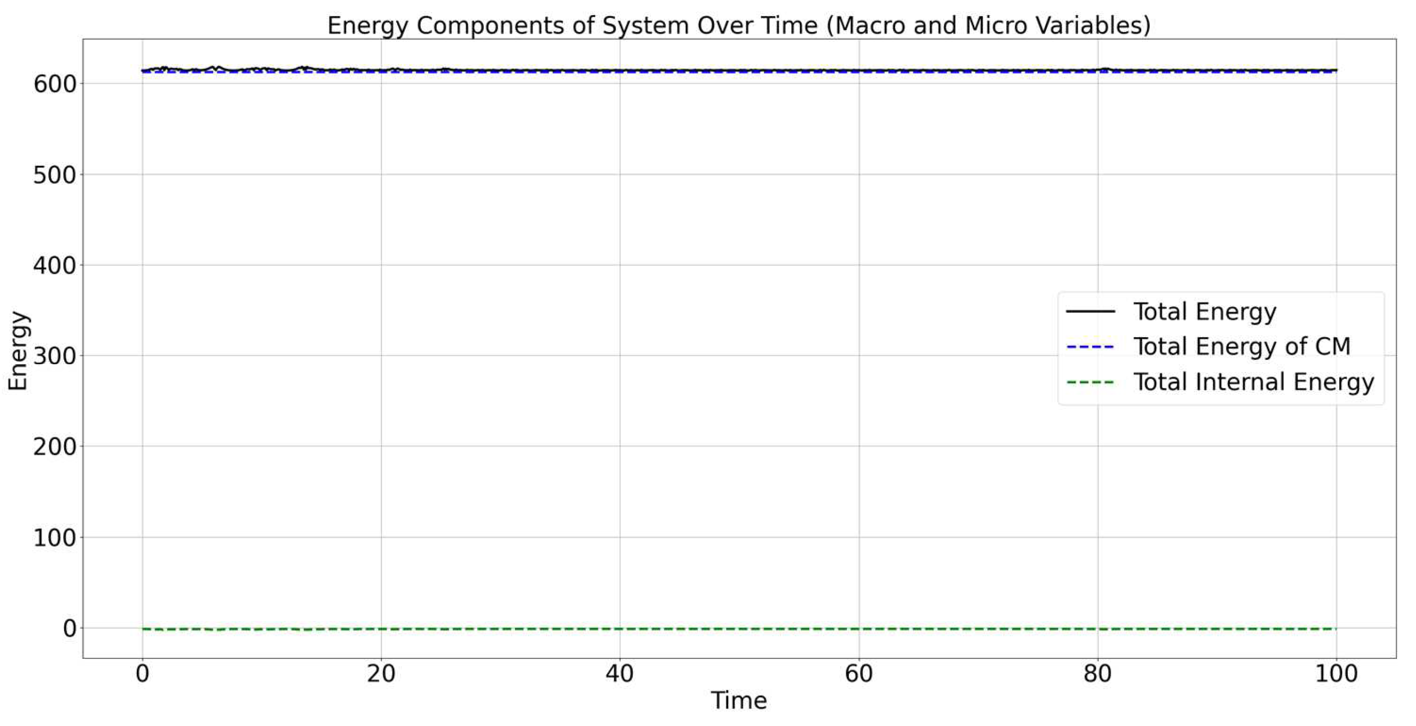
The total energy of the system (black line) remains constant over time, which indicates that the numerical model correctly conserves energy. The constancy of total energy also implies that there are no external forces or energy losses (e.g., due to friction) that would otherwise change the total energy.
The total energy of the CM (blue dashed line) remains nearly constant and is slightly above the total energy line. This suggests that most of the system’s energy is associated with the motion of the center of mass. The constancy of the energy of the CM also suggests that the energy involved in the system’s translation is stable and not significantly influenced by internal interactions.
The total internal energy (green dashed line) remains consistently lower compared to the other components, indicating that the internal interactions (both relative kinetic and potential energies) are relatively small compared to the energy of the center of mass.
The low value of internal energy means that the internal motion and interactions between particles contribute much less to the overall energy of the system compared to the collective movement of the entire system.
The total energy of the CM and total internal energy collectively contribute to the total energy of the system. The graph suggests that while there are small fluctuations in the energy of the CM and internal energy, these changes are balanced, maintaining the conservation of total energy.
The total energy of the system remains nearly constant, indicating that energy is conserved in the simulation and that there are no significant numerical errors or losses. The energy of the center of mass constitutes the dominant part of the system’s energy, indicating that the overall movement of the system is the most significant contributor to the total energy. The internal energy contributes relatively little compared to the energy of the CM, which suggests that the interactions between particles do not significantly impact the total energy, likely because the internal interactions are not intense enough to cause major energy shifts in the system. These findings illustrate that the model effectively captures the energy dynamics of both the macroscopic motion of the system (via the center of mass) and the microscopic interactions between particles, while preserving energy conservation over time.
4.3. D-Entropy Behavior
The behavior of D-entropy (SD) over time is shown in Figure 5. D-entropy measures the ratio of the change in internal energy to the total internal energy and helps describe the system’s progression towards thermodynamic equilibrium.
Figure 5 presents the evolution of D-Entropy over time, represented by a purple line. D-Entropy in this context measures the relative change in the internal energy of the system due to energy transfers within the particles. The plot shows fluctuations in D-Entropy values, oscillating between positive and negative values. These fluctuations indicate changes in the internal energy of the system, either increasing (positive values) or decreasing (negative values). The fluctuations are indicative of ongoing exchange processes within the internal degrees of freedom of the system.
During the initial phase (approximately the first 20 units of time), there is a higher magnitude of D-Entropy changes, with both positive and negative spikes being more pronounced.This indicates a period of energetic adjustment, likely due to the system transitioning from its initial state to a more settled state. The particles are undergoing significant interactions and energy redistribution as they find equilibrium positions.
As time progresses, the magnitude of fluctuations decreases, and the D-Entropy values become more stable, with smaller oscillations around zero.This suggests that the system is reaching a state of dynamic equilibrium, where the rate of energy exchange between particles becomes more uniform, and large deviations in internal energy are less frequent. Around t = 80, there is a noticeable spike in D-Entropy, followed by rapid stabilization, indicating a transient interaction or event that momentarily disturbed the energy balance before settling back.
Positive values of D-Entropy indicate that internal energy is increasing, meaning that energy is being added to the internal system. This could be due to energy transferred from kinetic to potential forms within the interacting particles. Negative values imply a loss of internal energy, often due to energy being redistributed away from internal forms—possibly into the kinetic energy of the center of mass or due to internal relaxation effects.
The fact that the fluctuations reduce over time indicates that the dissipative processes in the system are settling to a balanced state. The D-Entropy tends toward zero, implying minimal net change in internal energy over time, which is consistent with the system reaching a state of thermodynamic balance. These observations suggest that the system is moving towards a steady state, where energy exchanges still occur, but without significant net gains or losses in internal energy.
D-Entropy reflects the changes in internal degrees of freedom of the system, which is related to how energy is redistributed among particles. The initial high variability in D-Entropy suggests that the system undergoes significant reconfiguration and energy redistribution after the initial setup. This is common in systems that begin with random initial conditions, where particles take time to reach a relatively stable arrangement. As the system progresses, the fluctuations reduce in magnitude, which indicates a movement towards energy equilibrium. Negative D-Entropy values imply that the system experiences periods where energy is predominantly being transferred out of the internal interactions, while positive values suggest energy is being absorbed internally.
The fluctuating behavior of D-Entropy indicates an ongoing process of energy exchange between particles, with periods of gain and loss depending on their interactions. The system shows evidence of moving towards dynamic equilibrium, where D-Entropy oscillates around zero with decreasing amplitude, suggesting stabilization of energy exchanges. The overall trend suggests that internal energy redistribution within the system reaches a balance over time, consistent with the system approaching a thermodynamically stable state. This analysis provides insights into the internal dynamics of the system and helps in understanding the energetic processes that occur as the system evolves towards equilibrium.
4.4. System Dynamics and Equilibrium
The system undergoes an initial phase of high-energy fluctuation as it attempts to reach equilibrium. This is characterized by strong interactions between particles due to the Lennard-Jones potential, which results in rapid changes in relative kinetic and potential energies.
Over time, the system achieves a dynamic equilibrium, where internal energy fluctuations are reduced, and the D-Entropy settles around zero, indicating minimal net changes in internal energy.
Throughout the simulation, the total energy of the system is conserved, with changes in individual energy components being balanced by corresponding changes elsewhere. The trajectories demonstrate complex interactions under the influence of both gravity and inter-particle forces. The resulting paths and energy fluctuations highlight the impact of the Lennard-Jones potential in driving non-linear and chaotic behavior.
The behavior of D-Entropy provides insights into the system’s approach to equilibrium, with initial fluctuations giving way to stable energy exchanges as the system reaches a balanced state.
These results provide a comprehensive understanding of the system’s behavior, showing the interplay between gravitational forces, inter-particle interactions, and energy conservation, with D-Entropy serving as a valuable metric for tracking internal energy dynamics.
4.5. Deviation of Total Energy Over Time
Figure 6 illustrates the deviation of the total energy of the system over time. This deviation represents how much the calculated total energy of the system fluctuates from its expected value, which, in an ideal energy-conserving system, should remain constant. The deviation of total energy provides important insights into the accuracy of the numerical integration and the stability of the simulation. Relative deviation percentage=0.6647368688422619%
4.6.1. Initial Fluctuations and System Stabilization
During the initial phase (up to approximately 20 units of time), there are noticeable large deviations in total energy, reaching values up to 4 units. This is consistent with the system undergoing rapid energetic adjustments from its initial random state. Particles experience strong initial forces, including both repulsive and attractive interactions due to the Lennard-Jones potential, causing energy to fluctuate significantly.
As time progresses, the energy deviation decreases, indicating that the system is moving towards a more stable state. The amplitude of these fluctuations gradually diminishes, settling around a relatively small range after the initial chaotic period. This suggests that the system reaches a dynamic equilibrium, where energy exchanges are balanced, and the rate of fluctuations becomes considerably lower.
4.6.2. Possible Sources of Energy Deviation
The observed deviations in total energy are also influenced by numerical errors inherent in the integration method. While the Velocity-Verlet method, used for numerical integration, is known for its good energy conservation properties, it is not entirely free of error, especially during highly dynamic and non-linear interactions at the beginning of the simulation.
The complexity of the Lennard-Jones interactions, especially during close particle encounters, leads to rapid energy changes. These rapid interactions are more difficult to resolve accurately, which can lead to spikes in the total energy deviation.
4.6.3. Insights into System Behavior
The transition from large initial deviations to smaller, more controlled deviations reflects the system’s progress towards stability. The significant energy deviations during the early phase align with the strong fluctuations in D-Entropy observed in Figure 5, which highlights a period of intense energy redistribution as the system searches for equilibrium.
The reduction in energy deviation over time demonstrates the effectiveness of the numerical scheme in maintaining energy conservation once the system reaches a more stable configuration. After t ≈ 20, the energy deviation stays relatively low, which is an indicator of a well-behaved numerical model and a system approaching dynamic equilibrium.
The initial energy deviations are largely a result of the system’s transition from a far-from-equilibrium state. During this phase, particles interact strongly, leading to rapid changes in internal energy and correspondingly higher deviations.
As the simulation progresses, energy conservation improves, and the deviation stabilizes to smaller values, suggesting that the system has reached a balanced state where internal and external forces are in equilibrium.
The overall trend in energy deviation provides an important measure of the accuracy and stability of the numerical model and helps verify the system’s progression towards energy balance and equilibrium.
This analysis of total energy deviation contributes to understanding how the system evolves from an initial, chaotic state towards a stable equilibrium, and it validates the reliability of the numerical methods used for this study.
5. Discussion
5.1. Energy Dynamics and Conservation
The results of this study demonstrate the dynamics of a system of five particles under the influence of both gravitational forces and internal Lennard-Jones interactions. One of the key observations is the conservation of total energy within the system, even as energy components fluctuate between different forms (e.g., kinetic, potential, internal).
The total energy of the system remains nearly constant over time, indicating that the simulation has properly implemented energy conservation. This is crucial for understanding the system’s behavior, as it validates that no energy is artificially lost or added during numerical integration.
The energy components, such as the kinetic energy of the center of mass and the internal potential energy, demonstrate significant fluctuations, especially during the initial stages. These fluctuations reflect the redistribution of energy as particles move under the influence of gravitational pull and mutual interactions.
The analysis of energy conservation also reveals the efficiency of the numerical methods employed, such as the Velocity-Verlet algorithm, which is well-suited for maintaining energy conservation in systems dominated by non-linear interactions.
5.2. Initial Fluctuations and Approach to Equilibrium
The initial fluctuations observed in the D-Entropy plot provide insight into how the system transitions from an initial random configuration to a more stable equilibrium state. The strong oscillations in D-Entropy suggest a significant exchange of energy between the internal components of the system during the early stages of simulation.
During the initial phase, the particles are far from equilibrium, leading to rapid adjustments in their velocities and positions. The Lennard-Jones potential, with its combination of attractive and repulsive components, drives these changes as particles attempt to find stable configurations.
The large initial D-Entropy values highlight the energy redistribution occurring as particles experience both repulsion (due to close proximity) and attraction (at intermediate distances). This dynamic behavior ultimately results in the system reaching a state of dynamic equilibrium, where fluctuations in energy are minimized.
The damped oscillations of D-Entropy after the initial phase reflect the system’s approach to a steady state, where internal energy changes occur at a much slower rate, indicating that a stable configuration has been reached. This dynamic equilibrium suggests that while individual particle interactions continue, the system as a whole is balanced.
5.3. Particle Trajectories and Interaction Effects
The trajectories of the particles provide valuable information about the influence of both gravitational forces and Lennard-Jones interactions.
The gravitational force primarily drives the downward motion of the particles, resulting in a parabolic trajectory for each particle. However, deviations from a purely parabolic path indicate the influence of inter-particle forces.
The Lennard-Jones interactions lead to complex behaviors, including oscillatory motions and sharp changes in direction due to repulsion when particles come too close. The strong repulsive forces act like elastic collisions, preventing the particles from collapsing into each other and thereby contributing to the observed deviations.
The complexity of particle motion under both forces underscores the importance of considering non-linear interactions when analyzing multi-body systems. The oscillatory behaviors and non-linear trajectories are typical in systems governed by potentials like Lennard-Jones, which include both short-range repulsion and longer-range attraction.
5.4. D-Entropy and Thermodynamic Insight
The concept of D-Entropy was introduced as a means of quantifying the relative change in internal energy. The behavior of D-Entropy provides key insights into the thermodynamic evolution of the system.
During the simulation, periods of positive D-Entropy indicate phases where internal energy increases, likely due to particles moving closer together, thereby increasing relative potential energy. Conversely, negative D-Entropy values reflect a decrease in internal energy, potentially as particles move apart and reduce potential energy.
The trend toward smaller D-Entropy fluctuations over time suggests that the system is approaching a thermodynamic equilibrium. In this state, the rate of energy exchange between internal degrees of freedom and the center of mass becomes minimal, and the system reaches a more uniform energy distribution.
The use of D-Entropy provides a useful measure of the internal stability of the system and the efficiency of energy redistribution over time. The decreasing amplitude of D-Entropy suggests that the system has reached a point where the internal energy contributions are relatively stable, and major energy exchanges are no longer occurring.
5.5. Implications for Structured Body Dynamics
The results of this study provide a foundation for understanding the dynamics of structured bodies—systems that, unlike simple point masses, have internal degrees of freedom and complex interactions. The division of energy into components associated with the center of mass and those related to internal interactions is a key characteristic of structured bodies.
The internal energy dynamics captured by D-Entropy illustrate how energy is transferred within a structured system, providing insight into the thermodynamic stability and response to external forces.
The findings also highlight how structured systems interact with external forces, such as gravity, while managing internal energy, which is crucial for applications in fields like material science and astrophysics where structured bodies are common.
5.6. Limitations and Future Directions
While the current simulation effectively captures the energy dynamics and trajectory behaviors of the particles, several aspects could be further explored in future research.
Extended Interaction Potentials: The Lennard-Jones potential provides a good approximation for many types of molecular interactions, but other potentials, such as Morse or Coulombic potentials, could be explored to better understand the effects of different interaction types on system dynamics.
Dissipative Forces: The current study assumes conservative forces with no energy dissipation. Introducing dissipative forces (e.g., friction or damping) would help understand how energy is lost over time and how systems achieve true thermodynamic equilibrium.
Scaling Up the System: Increasing the number of particles would provide more insight into collective behaviors and phase transitions, which could be relevant in understanding complex systems such as granular materials or biological tissues.
5.7. Comparison of D-Entropy with Other Entropies
D-Entropy represents a unique approach to understanding the changes in internal energy within a system, particularly by capturing how energy redistributes among the internal degrees of freedom. It is useful in contexts where both micro-level interactions and macro-level dynamics need to be accounted for. Below, we compare D-Entropy with more conventional types of entropy, such as thermodynamic entropy, Shannon entropy, and Boltzmann entropy.
1) D-Entropy vs. Thermodynamic Entropy
Thermodynamic entropy, denoted typically as S, measures the degree of disorder or randomness in a thermodynamic system and is related to the number of accessible microstates. According to Prigogine [13], thermodynamic entropy is closely linked to the number of microstates and is suitable for equilibrium processes. It is a state function and is defined within the context of thermal equilibrium. D-Entropy, in contrast, measures the relative change in internal energy due to dynamic interactions in a system, capturing how energy flows between internal and external components. It is a measure that reflects changes in the energetic structure of a system rather than focusing directly on disorder or the number of states. Unlike thermodynamic entropy, which tends to increase according to the second law of thermodynamics, D-Entropy can have both positive and negative values, indicating increases or decreases in internal energy. This reflects energy exchange dynamics rather than simply measuring the system’s disorder.
2) D-Entropy vs. Shannon Entropy
Shannon [14] introduced entropy for assessing informational uncertainty. It measures the expected value of the information content and is often used to represent the information complexity of a system. D-Entropy is related to energetic changes in a physical system and describes how energy is redistributed among particles. It does not measure information content directly but could be interpreted in terms of how energy distributions impact the complexity of internal dynamics. While Shannon entropy considers the probability distribution of different outcomes (e.g., symbols or states), D-Entropy focuses specifically on the energetic outcome of interactions and the change in energy balance over time. In a sense, Shannon entropy could describe the configurational complexity, while D-Entropy is more focused on the energetic complexity of how energy shifts occur.
3) D-Entropy vs. Boltzmann Entropy
In Boltzmann’s classic work [15], entropy is related to the number of accessible microstates.Boltzmann entropy (SB) is defined as SB=kB ln(Ω) is the number of possible microstates corresponding to a particular macrostate, and kB is the Boltzmann constant. This entropy relates to the statistical properties of the microstates of a system and provides a bridge between microscopic and macroscopic thermodynamics. D-Entropy, unlike Boltzmann entropy, does not rely on counting microstates or analyzing statistical distributions. Instead, it captures dynamic energy changes over time, especially focusing on the exchange between internal degrees of freedom and external contributions.
Boltzmann entropy is often associated with the system’s approach to equilibrium, where the number of accessible microstates increases, resulting in an overall increase in entropy. D-Entropy, on the other hand, provides a more dynamic perspective, quantifying how internal energy changes can evolve even before equilibrium is reached.
4) Time Dependence and Dynamics
Research by Kazutinsky and Mamchur [2] emphasizes the importance of studying dynamic aspects of entropy in the context of nonequilibrium processes, which is also characteristic of D-Entropy.
Thermodynamic entropy generally increases monotonically in isolated systems, reflecting the irreversibility of natural processes and the tendency towards maximum entropy and equilibrium. D-Entropy is time-dependent and reflects non-equilibrium dynamics. The fact that D-Entropy can be both positive and negative means it can capture transient states where energy is redistributed, often before the system settles into an equilibrium.
For complex systems undergoing rapid changes, D-Entropy provides a useful measure of the rate and nature of internal energy redistribution, giving insights that static measures like traditional entropy might miss, particularly during far-from-equilibrium processes.
5) Applicability in Different Contexts
D-Entropy is particularly useful in understanding the energetic dynamics of systems that are interacting and evolving over time, where energy redistribution is a critical aspect of the system’s behavior. It is beneficial for studying structured systems where internal energy changes have a direct influence on overall dynamics, such as in astrophysical bodies, complex materials, or biological structures.
In Anderson’s article [3], the importance of considering both microscopic and macroscopic aspects in physical systems is highlighted, making D-Entropy a useful tool for studying energy dynamics in complex systems.
In conclusion, D-Entropy provides a dynamic perspective that differs significantly from the more traditional entropies by focusing on energy flows within a system. It helps in understanding how structured systems evolve over time and how internal degrees of freedom interact with external forces, making it a valuable tool in non-equilibrium dynamics, complex systems, and scenarios involving significant energy redistribution.
The discussion highlights the key dynamics of the system, including energy conservation, particle trajectories, and the role of D-Entropy in understanding internal energy changes. The initial fluctuations in D-Entropy reflect the system’s energetic adjustment, while the eventual reduction in fluctuations suggests a movement towards dynamic equilibrium.
The implications for structured body dynamics are significant, as this study illustrates how internal interactions and external forces affect the system’s behavior. Future work could focus on expanding the scope of interactions and introducing dissipative effects to provide a more comprehensive understanding of structured systems in various physical contexts.
6. Conclusion
This study explored the dynamics of a system of five interacting particles under the influence of gravitational forces and internal interactions modeled using the Lennard-Jones potential. The primary focus was on analyzing the redistribution of energy among different components of the system and investigating the concept of D-Entropy as a measure of changes in internal energy. Based on numerical simulations and the analysis of the results, the following conclusions can be drawn:
- 1)
- Energy conservation was successfully demonstrated throughout the simulation. The total energy of the system remained constant over time, despite significant fluctuations between different energy components. This confirms the correctness of the chosen numerical method and approach for modeling interacting particles.
- 2)
- Initial energy and D-Entropy fluctuations reflect the system’s attempt to transition from an unstable initial state to a more stable configuration. During the early stages, significant changes in internal energy components were observed, driven by energy redistribution between potential and kinetic forms due to attractive and repulsive particle interactions.
- 3)
- Particle trajectories exhibited complex behavior under the influence of gravitational and inter-particle forces. Gravity led to the downward motion of particles, while internal Lennard-Jones interactions caused deviations and oscillations in the trajectories. This emphasizes the importance of accounting for non-linear interactions when modeling multi-body systems.
- 4)
- D-Entropy proved to be a useful tool for tracking changes in internal energy and assessing the thermodynamic state of the system. In the early stages, significant D-Entropy fluctuations indicated intense energy exchange between components, while a reduction in fluctuation amplitude over time signaled that the system reached dynamic equilibrium.
- 5)
- Implications for structured bodies lie in the fact that the division of energy into components associated with the center of mass and internal interactions helps to better understand the behavior of more complex systems with internal structures. Systems such as materials with complex microstructures or celestial bodies with internal mass distribution can be effectively described using the presented approach.
Future Research Directions
This study identified several directions for further work:
Introducing dissipative forces into the system, such as friction, would provide a better understanding of how energy dissipates and how the system achieves true thermodynamic equilibrium. Using other interaction potentials, such as the Coulomb or Morse potential, could expand our understanding of how different types of interactions affect the system’s dynamics. Increasing the number of particles and scaling up the system would help to identify collective effects and phase transitions, which would be useful for modeling complex materials and biological systems.
In conclusion, this study demonstrates that using concepts like D-Entropy, along with a detailed analysis of energy components, are important steps in understanding the dynamics of complex systems with internal interactions. The presented methods and conclusions can be useful in various fields, from materials science to astrophysics, where it is necessary to consider interactions between multiple particles and the distribution of energy within the system.
Funding
This research was funded by Committee of Science of the Ministry of Science and Higher Education of the Republic of Kazakhstan, grant number AP19174928 “Study of ionospheric irregularities by methods of nonlinear analysis”.
Conflicts of Interest
The authors declare no conflicts of interest.
References
- Prigogine, I. Understanding the Complex; World: Moscow, 1990; 342 p. [Google Scholar]
- Kazutinsky, V.V.; Mamchur, E.A. (Eds.) Evolutionism and Global Problems; Russian Academy of Sciences, Institute of Philosophy: Moscow, 2007; 253 p. [Google Scholar]
- Anderson, P.W. More Is Different. Science 1972, 177, 393. [Google Scholar] [CrossRef] [PubMed]
- Goldstein, H. Classical Mechanics; Nauka: Moscow, 1975; 416 p. [Google Scholar]
- Lanczos, C. The Variational Principles of Mechanics; Mir: Moscow, 1965. [Google Scholar]
- Landau, L.D.; Lifshitz, E.M. Mechanics; Nauka: Moscow, 1973; 215 p. [Google Scholar]
- Zaslavsky, G.M. Stochasticity of Dynamical Systems; Nauka: Moscow, 1984; 273 p. [Google Scholar]
- Greenstein, J.; Zajonc, A. The Quantum Challenge: Modern Research on the Foundations of Quantum Mechanics; Intellect: Dolgoprudny, 2012; 432 p. [Google Scholar]
- Somsikov, V.M.; Andreev, A.B. On the Criteria for the Transition to a Thermodynamic Description of the Dynamics of Systems. News University. Series Physics 2015, 7. [Google Scholar] [CrossRef]
- Somsikov, V.M. D-Entropy in Classical Mechanics. 14th Chaotic Modeling and Simulation International Conference; Springer: Cham, 2022. [Google Scholar] [CrossRef]
- Hu, W.; Song, M.; Deng, Z. Structure-preserving properties of Störmer-Verlet scheme for mathematical pendulum. Applied Mathematics and Mechanics 2017, 38, 1225–1232. [Google Scholar] [CrossRef]
- Lennard-Jones, J.E. “Cohesion”, Proceedings of the Physical Society (1931).
- Prigogine, I. Understanding the Complex. Moscow: World, 1990.
- Shannon, C. E. “A Mathematical Theory of Communication.”. The Bell System Technical Journal, 1948, 27, 379–423. [Google Scholar] [CrossRef]
- Boltzmann, L. Lectures on Gas Theory. University of California Press, 1964.
Figure 1.
Trajectories of Particles in 2D (Free Fall with Lennard-Jones Interaction).
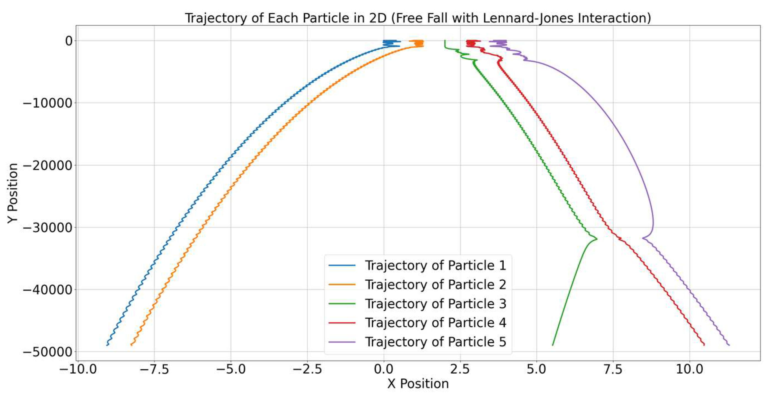
Figure 2.
Energy Components of System Over Time (Macro Variables).
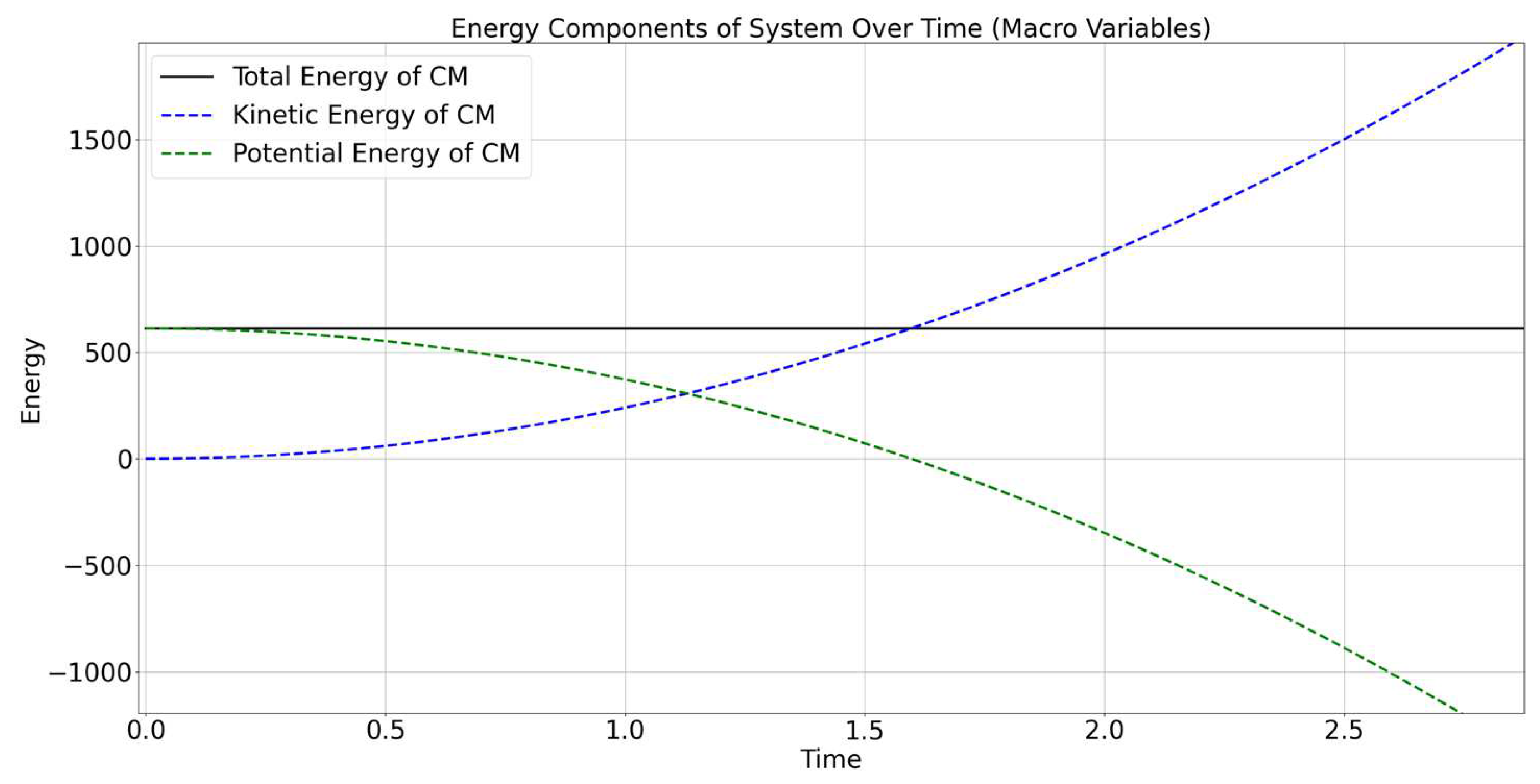
Figure 3.
Energy Components of System Over Time (Micro Variables).
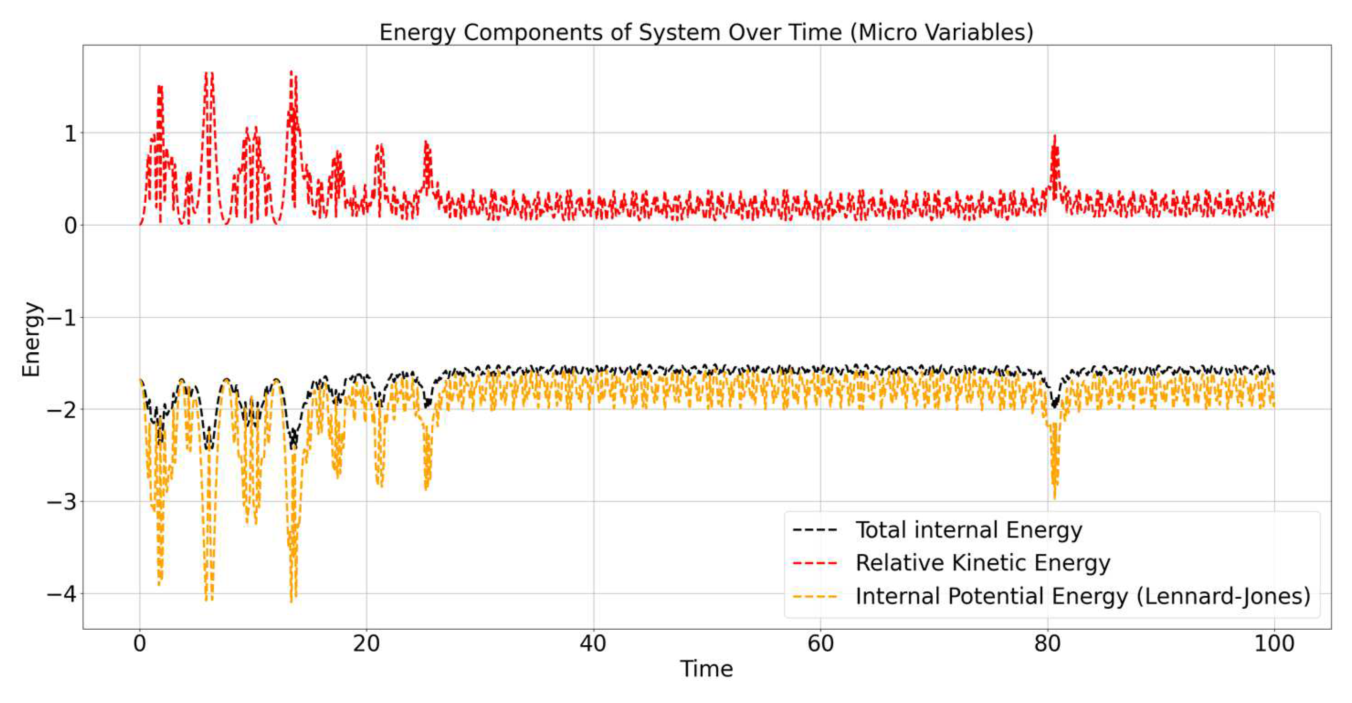
Figure 5.
D-Entropy Over Time.
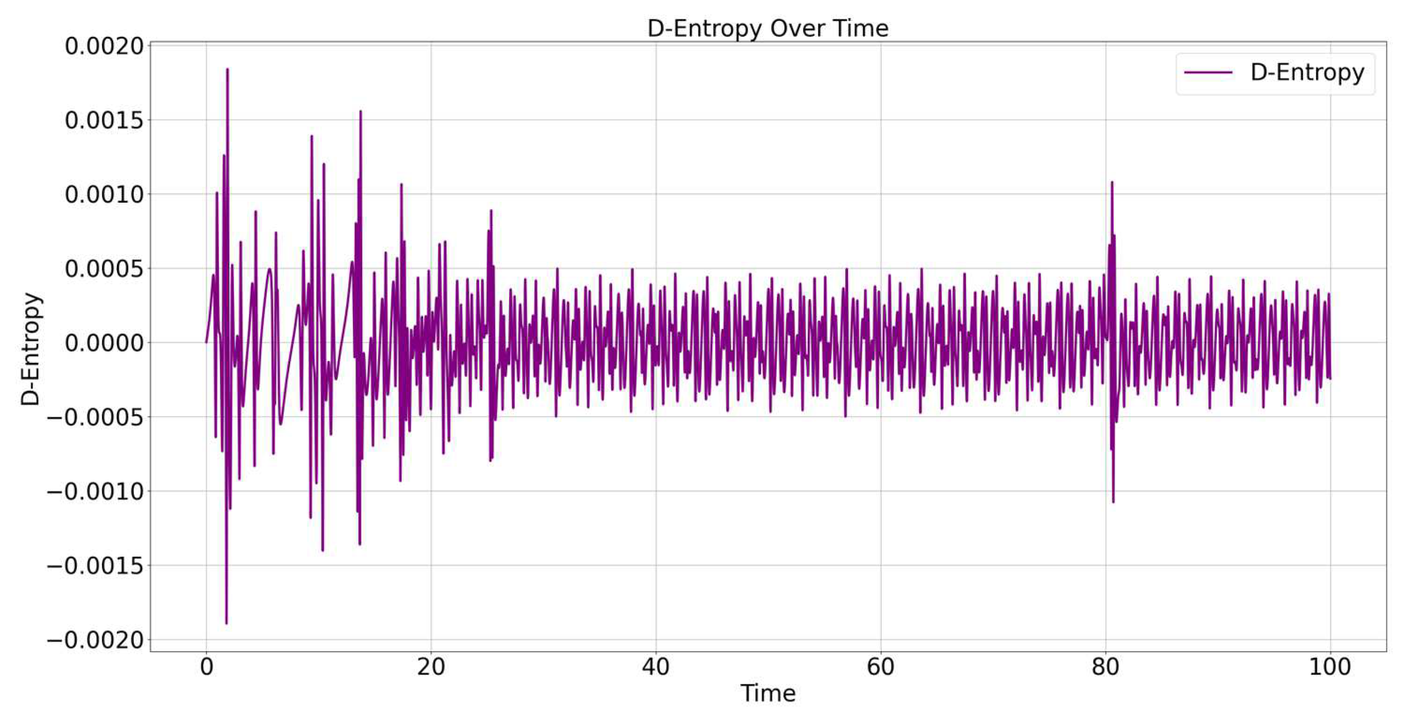
Figure 6.
Deviation of the total energy of the system over time.

Disclaimer/Publisher’s Note: The statements, opinions and data contained in all publications are solely those of the individual author(s) and contributor(s) and not of MDPI and/or the editor(s). MDPI and/or the editor(s) disclaim responsibility for any injury to people or property resulting from any ideas, methods, instructions or products referred to in the content. |
© 2025 by the authors. Licensee MDPI, Basel, Switzerland. This article is an open access article distributed under the terms and conditions of the Creative Commons Attribution (CC BY) license (http://creativecommons.org/licenses/by/4.0/).
Copyright: This open access article is published under a Creative Commons CC BY 4.0 license, which permit the free download, distribution, and reuse, provided that the author and preprint are cited in any reuse.


