
Submitted:
25 December 2024
Posted:
26 December 2024
You are already at the latest version
Abstract
Structural health monitoring (SHM) in Composite Fiber Reinforced Polymer (CFRP) structures is essential to ensure safety and reliability during service, particularly in critical industries such as aerospace and wind energy. Traditional methods of analysing Acoustic Emission (AE) signals in the time domain often fail to accurately detect subtle or early-stage damage, limiting their effectiveness. The present study introduces a novel approach that integrates frequency-domain analysis using Fast Fourier Transform (FFT) with deep learning techniques for more accurate and proactive damage detection. AE signals are first transformed into the frequency domain, where significant frequency components are extracted and used as input for an autoencoder network. The autoencoder reduces the dimensionality of the data while preserving essential features, enabling unsupervised clustering to identify distinct damage states. Temporal damage evolution is modeled using Markov chain analysis to provide insights into how damage progresses over time. The proposed method achieves a reconstruction error of 0.0017 and a high R-squared value of 0.95, indicating the autoencoder's effectiveness in learning compact representations while minimising information loss. Clustering results, with a silhouette score of 0.37, demonstrate well-separated clusters that correspond to different damage stages. Markov chain analysis captures the transitions between damage states, providing a predictive framework for assessing damage progression. These findings highlight the potential of the proposed approach for early damage detection and predictive maintenance, significantly improving the effectiveness of AE-based SHM systems in reducing downtime and extending component lifespan.
Keywords:
Structural Health Monitoring (SHM)
; Acoustic Emission (AE)
; Fast Fourier Transform (FFT)
; autoencoders
; deep learning
; clustering
; Markov chain analysis
; Composite Fiber Reinforced Polymer (CFRP)
; damage detection
; predictive maintenance
1. Introduction
Fibre Reinforced Polymers (FRPs) are the materials of choice for a wide range of industrial structural components where light weight, high stiffness and high strength are required. FRPs often exhibit superior performance in comparison with metallic alloys, without risk of corrosion or Stress Corrosion Cracking (SCC) due to exposure to the prevailing environmental conditions of the application. The exact physical properties of these are dependent on the specific combination of matrix polymer resin material and type of reinforcing fibres. This allows versatility in the mechanical properties of the FRPs allowing their tailoring according to the requirements of a particular application. However, their inspection and monitoring, is also more complex due to the anisotropic microstructure and the more complex damage modes affecting FRPs [1].
Traditionally, damage assessment in FRPs is carried out using appropriate Non-Destructive Testing (NDT) techniques. One such technique commonly employed for the inspection of FRPs is Ultrasonic Testing (UT) [2]. UT allows the precise localisation of existing damage or defects within an FRP structure but is adversely affected by high attenuation of the interrogating ultrasonic beam. Other issues are associated with the deployment of the ultrasonic probe, which requires it to be directly coupled with the surface of the test piece, also necessitating that the surface is clean and has low roughness. Examples of FRP components requiring inspection include Wind Turbine Blades (WTBs), aircraft aerofoils, composite pipes, etc., each of which pose their own inspection challenges. Wind turbines are installed in remote locations and often offshore with WTBs being in excess of several metres high from the ground. This renders inspection with conventional NDT techniques, such as UT, very challenging. Additionally, the use of paints and coatings, may adversely affect transmissibility of UT signals. A significant shortcoming is that ultimately UT can only detect damage that has already occurred when inspection takes place. Thus, it offers no warning during damage initiation and subsequent evolution between inspection intervals. Infrared (IR) thermography is an alternative NDT method but generally it has limitation in terms of depth of penetration. Moreover, it is better suited for detection of volumetric defects, close to the surface, rather than detection of cracks, which is more difficult to achieve [3]. The combination of NDT techniques can maximise the likelihood of detection of defects in FRPs. However, real-time evaluation is still not straightforward. The application of online real-time SHM on FRP structures using AE can provide useful information during in-service operation by detecting, localising and characterising damage initiation and subsequent evolution.
Unlike comparable NDT methods, AE does not rely on the direct excitation of the material. It is based instead on a passive monitoring approach relying on the response of the material to the occurrence internal physical irreversible changes. These events generate transient elastic wave, which in anisotropic plate structures, such as FRPs, propagate in the form of Lamb waves [4]. Lamb waves propagating along the plate structure are detected using piezoelectric sensors, with the sensing elements made of lead zircoate titanate. Piezoelectric sensors are able to convert the mechanical deformations occurring on the surface of the test-piece to electric signals which can be subsequently digitised, analysed and stored. AE signal assessment is typically based on the evaluation of the acquired signals, analysing features and trends in the time domain. Some Key Parameter Indicators (KPIs) used for the evaluation of AE signals are the peak signal amplitude of a detected AE event, AE energy and rise time of the signal [5]. However, assessment using such KPIs makes the identification of the specific damage mechanism very complex and not particularly reliable. The application of Digital Signal Processing (DSP) techniques, such as the Fourier series within a Fast Fourier Transform (FFT) [6], allow for more in-depth and reliable analysis of the actual waveforms captured. Such analysis permits the evaluation of the input signal in the frequency-domain representation providing valuable information regarding the specific damage mechanism to which the signal is associated.
The integration of machine learning and deep learning into AE analysis marks a significant evolution in structural health monitoring, addressing the constraints of traditional methods. Recent studies have explored supervised learning approaches for AE-based damage detection, demonstrating improved accuracy in time-domain signal classification. Recent advancements in Artificial Intelligence (AI), particularly in Multitask Learning Deep Neural Networks (MTL-DNN), have demonstrated substantial potential for modal identification of large-scale structures in SHM. In this context, MTL-DNN models, like the one proposed by García-Macías et al. [7] were designed to reduce computational demands while improving the accuracy of damage assessments. For instance, the MTL-DNN applied to the Méndez-Núñez Bridge in Spain reduced modal identification time from 57 minutes to just 0.4 seconds, with modal assurance criterion (MAC) values close to 1.00, signifying almost perfect correlation between the modes identified by the model and traditional methods.
In other studies deep learning implementations for AE source localization addressed restricted and imbalanced datasets from fiber-optic AE sensors used in SHM [8]. Using generative adversarial networks (GANs) for data augmentation and an inception-based neural network for regression, the proposed approach localized precisely with one sensor. The augmented dataset delivered 83% fidelity and 50% error reduction over non-augmented models, improving damage identification and predictive maintenance in complex infrastructures. Also, on the time domain, studies have achieved great results by utilizing hybrid approaches. A real-time deep learning framework, combining CNNs and LSTM, for diagnosing composite impact damage in SHM was able to to categorize damage into minor, intermediate, and severe failure [9]. Barile et al. [10] proposed a deep learning framework utilizing pre-trained CNN models (AlexNet, SqueezeNet) and a new simplified CNN model to classify and characterize the mechanical behavior of AlSi10Mg components during tensile testing. AE signals were recorded from specimens built using Selective Laser Melting with varying bed orientations. The study applied time-frequency analysis using continuous wavelet transform (CWT)-based spectrograms to classify damage in three categories. The results show that the new CNN model achieves 100% classification accuracy in less time compared to AlexNet and SqueezeNet, highlighting its efficiency for AE signal classification. Finally, Sikdar et al. [11] investigated SHM for lightweight composite structures by utilzing a data-driven deep learning approach. AE signals from piezoelectric sensor newtwork on a composite panel were processed with continuous wavelet traform to extract time-frequency scalograms. A CNN was proposed to classify damage-source regions based on these scalograms, demonstrating high accuracy in training, validation, and testing, even for unseen datasets. The use of peak-signal scalogram data significantly improved the performance of the damage-source classification by achieving an accuracy of 97.34%.
Nonetheless, AE analysis implementation frequently encounters obstacles because to inconsistencies between simulated and empirical data, along with imbalances in datasets characterized by paucity of late-stage fracture data. Huang et al. [12] presented a domain adaptation framework to address these problems, utilizing sophisticated feature extraction methods and a dual-loss optimization approach to align the data distributions of the source (simulated) and target (experimental) datasets. The model adeptly categorized stages of crack growth by integrating Finite Element Method (FEM) simulations with actual data from a Fiber Bragg Grating Fabry–Perot Interferometer (FBG-FPI) sensor system. The results illustrated the model's flexibility and resilience, attaining elevated classification accuracy and equitable performance across imbalanced datasets. Zhang et al. [13] presented an innovative damage identification method which integrated double-window principal component analysis (DWPCA) with AI techniques, specifically random forest (RF) and bidirectional gated recurrent unit (BiGRU). The method employed multiple temporal window scales (e.g. annual, seasonal, and monthly) to derive damage-sensitive eigenvectors, subsequently utilized as inputs for the AI algorithms. The findings demonstrated that the integrataed DWPCA eigenvectors improved damage identificaiton precision, with over 95% accuracy, despote constrained training data and noise interference.
However, these methods often overlook the potential of frequency-domain features and struggle to track temporal damage evolution effectively. Existing research highlights the need for unsupervised techniques capable of capturing both frequency and temporal dynamics of AE signals. This gap underscores the importance of innovative frameworks that leverage deep learning for holistic AE signal analysis and damage progression monitoring.
In light of the limitations posed by traditional time-domain-based damage detection methods and the challenges in accurately tracking damage progression in CFRP structures, this study presents a novel, multi-phase approach that integrates frequency-domain analysis, deep learning autoencoders, clustering, and Markov chain analysis. By transforming AE signals using FFT and employing autoencoders [14] for dimensionality reduction, the proposed method effectively captures essential frequency components and identifies distinct damage states through unsupervised clustering. The subsequent application of Markov chain analysis [15] models the temporal evolution of these damage states, offering predictive insights into damage progression. This integrated framework addresses the current research gaps by providing a robust, unsupervised method for early damage detection and predictive maintenance, thereby enhancing the reliability and lifespan of critical components in industries like wind energy and aerospace. The contributions of this work not only advance the state-of-the-art in AE-based SHM but also offer a practical, scalable solution for real-time damage monitoring.
The rest of the paper is organized as follows: Section 2 describes the materials and methods used in the study, including the experimental setup, data collection, signal pre-processing, FFT transformation, and the deep learning techniques employed. Section 3 presents the results of the analysis, including damage detection, clustering, and temporal damage evolution. Section 4 discusses the findings, highlights the contributions of the proposed method, and situates them within the context of existing research. Finally, Section 5 provides the conclusions and outlines potential directions for future research.
2. Materials and Methods
This section outlines the methodology employed in the study (Figure 1), detailing the steps taken from data acquisition to the analysis of damage evolution in Composite Fiber Reinforced Polymer (CFRP) structures. It begins with an overview of the experimental setup and the procedures used for data collection. The subsequent phases cover the signal pre-processing and transformation of AE data from the time domain to the frequency domain using Fast Fourier Transform (FFT), followed by the application of deep autoencoder networks for learning compact representations of the processed signals. The latent space representations obtained from the autoencoder are then subjected to unsupervised clustering to identify distinct damage states. Visualisation techniques are employed to interpret the results, and finally, Markov chain analysis is used to model the temporal evolution of damage. Each stage of the methodology contributes to a comprehensive framework for detecting and monitoring damage progression in CFRP structures.
2.1. Experimental Setup
CFRP and GFRP coupons were used in mechanical tensile and three-point flexural tests were carried out as part of the Horizon 2020 Carbo4Power project. Collection of the AE data utilised for initial analysis and as input for model creation was completed through monitoring during the mechanical tests. Specific focus was placed upon CFRP, which are employed for the reinforcing spar during WTB manufacturing. The reinforcing spar is the main load-bearing component of the WTB. From the AE data captured during tensile and flexural testing it was possible to establish the relationship between AE response and associated damage mechanisms developing from the healthy condition of the material up to its final failure.
Tensile testing was performed using an electro-mechanical testing machine manufactured by Zwick Roell, model 1484, with a 200 kN load cell. The extensometer length was set to 10 mm and the crosshead movement speed was set to 2 mm/min. Test coupons with dimensions 250mm long by 25 mm wide were used for the tensile tests, with a thickness range 1.03-1.33 mm. These had a laminated layered structure with fibre direction of [[0/45/QRS/-45/90], where the QRS are Quantum Resistive Sensors in the shape of wires with a diameter comparable to that of the fibres. QRS are internally positioned, interlaminar, sensors for direct measurement of strain, temperature and humidity developed as part of the Carbo4Power project. End-tabs were used to allow for the proper application of the grip force during loading. Three-point bending testing was carried out using a Dartec Universal Mechanical Testing Machine, with a 50 kN load cell and a crosshead movement speed of 1 mm/min. Test coupons with dimensions 150 mm long by 25 mm wide and a thickness range of 1.15-1.32 mm. Again, these example coupons were of a layered laminated structure, with layup of [0/QRS/45/-45/90]; due to the nature of the specific mechanical testing no end tabs were required.
2.2. Data Collection
The data collection was performed using two R50αa narrow band resonant piezoelectric sensors manufactured by Physical Acoustics Corporation. The operational frequency range of the R50α sensors is from 150kHz to 500kHz. The sensors were mounted on the same side of the samples at each end using araldite two-component epoxy adhesive as illustrated in Figure 2.
The outputs of the sensors were amplified in two stages, a 40dB pre-amplification followed by another 9 dB using a bespoke 4 channel variable gain amplifier manufactured by Feldman Enterprises Ltd. The amplified signal was filtered at 500kHz for anti-aliasing purposes and was digitised using a 4 channel 16-bit National Instrument 9223 Compact Data Acquisition (NI-cDAQ) module. The NI-cDAQ module was connected to a very small Intel Next Unit of Computing (NUC) computer using a cDAQ-9171 via a USB port. The data acquisition was performed using bespoke software written in MATLAB and developed in house using NI-DAQmx which was hosted on the NUC computer. The recorded datasets were captured at 1MSamples/s per channel periodically for 5 second with a 1 second delay between each recording. Figure 3 illustrates a raw dataset recorded from a sample under 3-point flexural testing up to failure.
2.3. Signal Pre-Processing and FFT Transformation for Time-to-Frequency Domain Analysis
In the first phase of the methodology, the AE signals, initially captured in the time domain, are transformed into the frequency domain using FFT. This transformation is essential for revealing key frequency components associated with different types of damage that may not be as evident in the time domain. After the FFT is applied to each windowed signal, the mean FFT across the windows is calculated to create a representative frequency spectrum for the entire signal. To focus the analysis on the most relevant frequency components and filter out noise or insignificant variations, a thresholding technique is employed. In this case, a threshold is applied to the mean FFT values, with the threshold set at 0.01. This value was carefully chosen to retain significant frequency components while discarding those with lower amplitude, which are more likely to represent noise or non-damage-related fluctuations. The threshold ensures that only the most critical frequencies, those indicating potential damage, are passed on to the next phase of the analysis. Specifically, the thresholding is performed as follows: any frequency component in the mean FFT spectrum that exceeds the 0.01 threshold is retained for further processing, while components below this threshold are removed. This process helps reduce the dimensionality of the data and ensures that only the most informative frequency components are used as input for the subsequent autoencoder phase. This phase is crucial for several reasons. First, it allows the system to filter out irrelevant data and focus on the signals most likely to indicate damage. Second, by applying the threshold on the mean FFT of windowed signals, the method accounts for the overall frequency behaviour of the signal over time, providing a more robust approach to identifying key frequency components. By filtering out lower-amplitude noise and emphasising higher-amplitude signals, this thresholding technique enhances the quality of the data input to the autoencoder, improving the overall accuracy of the damage detection process.
2.4. Learning Compact Representations Through Deep Autoencoder Networks
The training of the autoencoder represents a critical phase in the overall methodology, where the model learns to compress the input data into a lower-dimensional latent space and then reconstruct it with minimal loss of information [16]. The input data to the autoencoder consists of the FFT values, after the threshold implementation, carefully filtered to retain only the most significant frequency components. The primary objective of training the autoencoder is to learn a compressed representation of this data in the latent space, while minimising the reconstruction error between the input and output.
The autoencoder architecture consists of two main components: the encoder and the decoder . The encoder is responsible for mapping the high-dimensional input data to a lower-dimensional latent space. During this process, the encoder learns to identify key features in the data that are essential for representing the underlying structure of the signals, effectively reducing the dimensionality of the input. The dimensionality of the latent space is determined through hyperparameter tuning, ensuring that it is compact enough to be efficient, yet large enough to retain critical information about the damage-related frequency components. Once the data has been compressed into the latent space, the decoder is tasked with reconstructing the original input data from this lower-dimensional representation. The decoder mirrors the encoder, gradually upscaling the compressed data back into its original high-dimensional form. The success of this reconstruction is measured by the reconstruction error, which quantifies the difference between the original input and the reconstructed output. The goal of training is to minimise this error, ensuring that the latent space captures the most informative features of the data with minimal loss of fidelity.
The training process involves iteratively adjusting the weights of the encoder and decoder through backpropagation. The autoencoder is trained using mean squared error (MSE) as the loss function, which measures the average squared differences between the input and reconstructed output. By minimising MSE, the autoencoder learns to effectively encode the “thresholded” FFT data in a way that preserves its key characteristics, while discarding irrelevant noise and redundant information. During the training process, Bayesian optimisation was employed to fine-tune the hyperparameters of the autoencoder. This optimisation process explored various configurations, including the size of the latent space, the regularisation terms, and the number of training epochs, to find the optimal settings that resulted in the lowest reconstruction error. The use of L2 weight regularisation and sparsity constraints ensured that the autoencoder did not overfit the training data, promoting a more generalised model that performs well on unseen data.
The autoencoder’s architecture is designed with several key hyperparameters that control its performance. These included: (i) L2 weight regularisation to prevent overfitting by penalising large weights; (ii) Sparsity regularisation to enforce a constraint that encourages the latent space to have a sparse representation, meaning that only a few neurons are activated for any given input; (iii) Sparsity proportion, which controlled the degree of sparsity in the latent representation; (iv) Encoding dimension, which determined the size of the latent space and, therefore, the degree of compression and (v) maximum number of epochs, which defined the number of training iterations. The optimal values of these hyperparameters were identified using Bayesian optimisation, which efficiently searched for the best combination of parameters by balancing exploration and exploitation of the hyperparameter space. This process minimised the reconstruction error and ensured that the autoencoder learned an optimal latent space representation of the normalised FFT data.
The autoencoder’s performance has been evaluated by assessing the ability to accurately reconstruct the original input data from the latent space. The reconstruction error, measured in terms of MSE between the original and reconstructed signals, served as the primary metric for evaluating the model’s performance. The reconstructed signal for each window was compared to the original normalised FFT data , and the reconstruction error was calculated as:
where n is the number of frequency components in each FFT vector. A low reconstruction error indicated that the autoencoder has effectively learned to compress and reconstruct the key features of the data. In addition to the quantitative evaluation, qualitative assessment was also performed by visualising the reconstructed signals alongside the original FFT data. This visual comparison helped to ensure that the shape of the FFT, which was critical for clustering, has been preserved during the dimensionality reduction process.
2.5. Clustering in the Latent Space
Once the autoencoder has performed the dimensionality reduction, the next important step was clustering the latent representations of the AE data. Clustering helped reveal hidden patterns in the latent space, which can correspond to different damage-related events. This section explained the clustering methodology, evaluated its performance, and provided a theoretical background along with result visualisations. The latent space generated by the autoencoder reduced the normalised FFT-transformed AE data into a lower-dimensional space that preserved the most critical features. Each point in the latent space corresponded to a windowed segment of the AE signal, representing the key signal characteristics captured by the autoencoder.
corresponds to the matrix of the encoded features, where was the number of AE windows and was the dimensionality of the latent space (optimised during autoencoder training). The goal of clustering in this latent space is to group data points into clusters, where each cluster potentially represented a distinct damage event or state. We utilised then k-means clustering, as an unsupervised learning algorithm, to partition the data into clusters based on the latent representations of AE data. The k-means algorithm iteratively assigned each data point to one of the clusters, represented by centroids , to minimise the within-cluster sum of squares (WCSS), which is defined as:
The algorithm proceeded in two steps: (1) Assignment Step: Assign each data point to the nearest cluster centroid and (2) Update Step: Update the centroids as the mean of the points in their respective clusters. The Silhoutte Score has been utilised for the clustering evaluation. Furthermore, in order to improve initialisation, we employed K-means [17]. This method selected initial centroids in a way that spreaded them out, reducing the likelihood of poor clustering. The first centroid was selected randomly, and each subsequent centroid was chosen based on the distance from the nearest previously selected centroid. The probability of choosing point was:
where is the distance to the nearest centroid already chosen. This initialisation improved the likelihood of finding globally optimal clustering. After determining the optimal clusters, we were able to classify new AE signals. For a new set of encoded features each data point was assigned to the closest cluster centroid from the original clustering.
where is the encoded feature for a new data point and is the centroid of the -th cluster from the original k-means model.
2.6. Visualisation
After clustering latent space representations, it was crucial to visualise clusters to understand how they group and relate to time-series data. We plotted the mean frequency content of each signal over time and color-code the points according to their cluster. Visualisation provided insights into the structure and evolution of clusters, allowing us to assess the characteristics of AE signals in relation to material damage events. The mean frequency content is calculated as:
where n is the number of frequency components. The points are then plotted against time , with different colors representing clusters. In addition to the latent space clusters, we plotted the accumulated mean frequency for each cluster over time. This is the cumulative sum of the mean frequency content for signals within each cluster:
This time-dependent view revealed frequency trends for each cluster, showing signal characteristics at different stages of damage. In order to understand the spectral characteristics of each cluster, we computed the mean frequency content and its standard deviation :
where is the set of signals in cluster
2.7. Temporal Damage Evolution Using Markov Chain Analysis
To analyse the temporal dynamics of clusters, we modelled transitions between clusters using a Markov chain. This approach allowed us to capture the frequency and likelihood of AE signals transitioning between different clusters over time, providing insights into the evolution of damage states within the monitored structure. Each cluster represents a specific stage or type of damage, and the transitions between them help us understand how damage progresses, stabilises, or regresses. This captured how frequently AE signals transitioned between clusters, corresponding to different damage stages. The transition matrix is:
where is the number of transitions from cluster to and is the total number of transitions from cluster i to any other cluster, ensuring that the probabilities in each row of the matrix sum to 1.
This formulation allows us to calculate the relative likelihood of transitioning between clusters, effectively capturing the progression from one damage state to another, as well as the likelihood of remaining in the same state (self-transitions). The higher the value of, the more likely it is that an AE signal moves from state i to state j, while low values indicate rare transitions or relatively stable states. The transition matrix is visualised as a state transition diagram. The state transition diagram is a graphical representation of the clusters and the transitions between them. Each node in the diagram represents a cluster, while the arrows between nodes indicate the direction and magnitude of transitions between states. The thickness of each arrow is proportional to the transition probability between clusters, with thicker arrows indicating more frequent transitions. Self-transitions are also represented by loops at each node, indicating the probability that a signal remains in the same cluster (damage state) over time. This diagram provides a clear view of the overall flow between different damage stages, allowing for an easy interpretation of how the system evolves.
The Markov chain analysis offers valuable insights into the temporal progression of damage in CFRP structures. By examining the transition probabilities, we can make several important observations:
- Clusters with high self-transition probabilities (i.e., large values of are considered stable states. These clusters represent damage stages that persist for longer periods before transitioning to another state. For instance, if the probability of staying within Cluster 1 is high, it suggests that this stage of damage is more prolonged or stable.
- The transition probabilities between clusters reveal how damage evolves over time. For example, a high probability of transitioning from Cluster 1 to Cluster 2 would indicate that damage is progressing from an early-stage or less severe state (Cluster 1) to a more advanced or severe stage (Cluster 2). These transitions are critical for understanding how damage accumulates and the speed at which it progresses.
- The Markov chain also allows for the analysis of reversibility in damage progression. If there is a significant probability of transitioning back from Cluster 2 to Cluster 1, this could suggest that certain damage processes may stabilise or revert under certain conditions, such as cyclical loads. This could be indicative of periods where the structure is subjected to temporary stress without permanent damage progression.
By modelling the system as a Markov chain, we can use the transition probabilities to forecast future states of the system. For instance, if there is a high probability of transitioning from a stable damage state to a more critical one, maintenance activities can be scheduled preemptively, reducing the risk of unexpected failures.
2.8. Assignment of Frequency Ranges for Damage Mechanisms
For the assessment of damage using the frequency components contained with a given AE event signal, it is important that the identified peaks and features can be properly attributed to their respective source and hence, related damage mechanism. The relationship between energy and frequency is well established, with observed damage mechanisms within an FRP also generating signals with distinctive energy content, which is dependent on the relative interfacial strength. When assessing damage mechanisms, attempting to characterise them using a specific frequency value can result in significant inaccuracies particularly since the propagation of the wave with increasing distance from the source will result in signal attenuation but also frequency dispersion. Hence, assigning ranges to the associated frequencies from observations of the transformed spectra can contribute to the correct identification of the damage mechanism affecting a particular FRP component during damage initiation and subsequent evolution. Assigning accurately the frequency ranges associated with different damage mechanisms will allow the effective damage mechanism identification and monitoring of damage initiation and evolution in FRP components.
One way of achieving this, is through the evaluation of the peak observed frequency for an extracted AE event ([18,19,20]). In previous studies published on the subject, commercial software with automated analysis has been commonly used. Herewith, we have employed a custom-built AE system and associated software. As this only relies on fairly simple Digital Signal Processing (DSP) approaches, the process can be executed with high sensitivity, accuracy and robustness in a time-efficient manner, with required operations completed post-acquisition. When assessing this in a way that allows the relative density of the extracted peak frequencies to be obtained, clear bands can be observed within the analysed signals, considering both frequency versus elapsed time and measured magnitude.
The extraction of peak frequency allows for the assessment of the primary contributing phase within the captured waveform. Hence, information of the dominant damage mode for a given identified AE event can be obtained. Knowing the usual damage progression within the tensile loading of the test coupons assists also in the assignment of damage modes to the bands which can be seen to be present. Based on the damage mechanisms in FRPs, five distinct bands are expected to arise, one for each of the primary damage mechanisms.
Figure 4.
Examples of Peak Frequency Assessment of a Tensile Tested CFRP Sample Coupon; a) Time vs. Peak Frequency and b) Magnitude vs. Peak Frequency.
Figure 4.
Examples of Peak Frequency Assessment of a Tensile Tested CFRP Sample Coupon; a) Time vs. Peak Frequency and b) Magnitude vs. Peak Frequency.
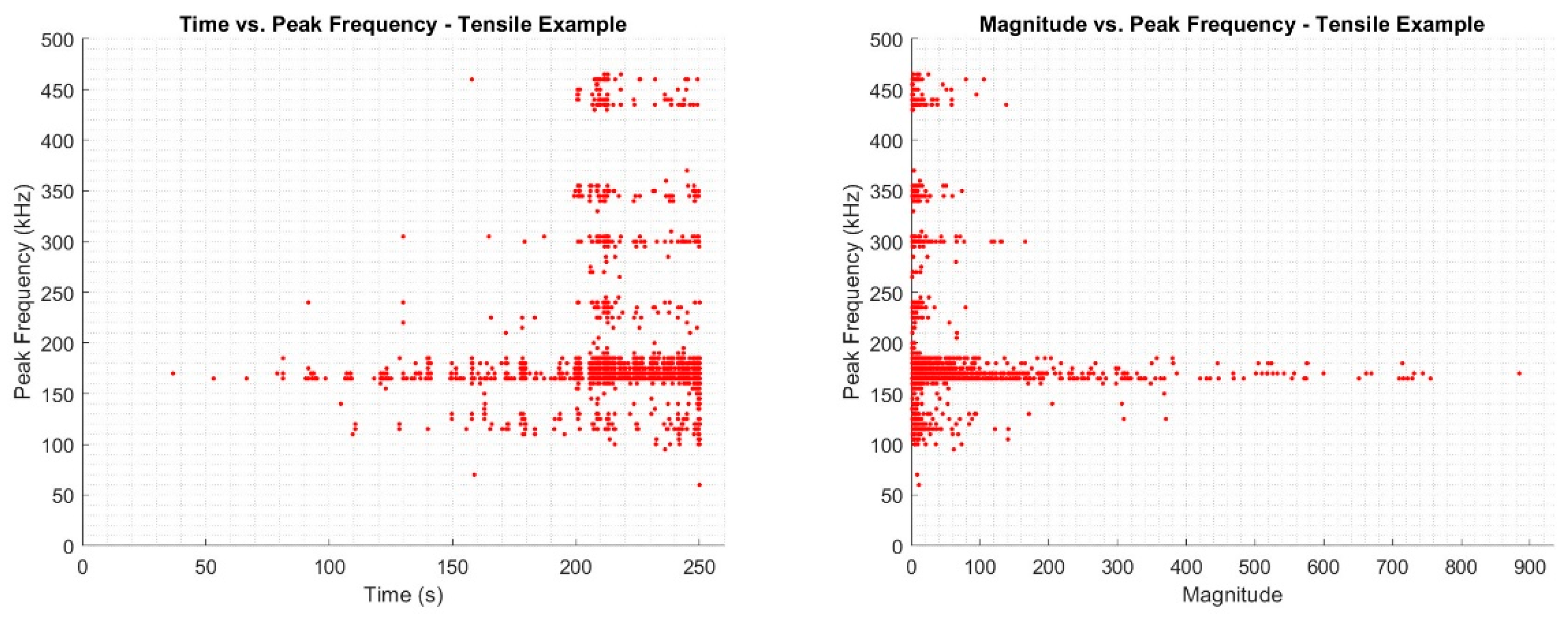

Table 1.
CFRP Damage Type and Assigned Frequency Ranges.
| Damage Mode | Frequency Range (kHz) |
|---|---|
| Matrix Cracking | 100 - 200 |
| Delamination | 200 – 250 |
| Debonding | 250 – 325 |
| Fibre Breakage | 325 – 400 |
| Fibre Pullout | 400 – 500 |
Peak frequency values identified below 100 kHz have been designated as anomalous, likely resulting from noise or from the misidentification of an AE event as damage, also typically associated with relative low signal amplitude. Matrix cracking has been assigned to the lower frequency range of 100-200 kHz. This extended range can be attributed to different directional behaviour associated with matrix cracking within the samples tested, not only in relation to the fibre direction in relation to the individual laminates which can give rise to both longitudinal and transverse matrix cracking. Also, the through-thickness matrix cracking, with cracks propagating perpendicular to the general plane of the material. The frequency ranges identified were observed across all samples tested, for both tensile and flexural testing. Hence, these frequency ranges can be employed for the evaluation of damage for materials tested. However, it is noted that the exact frequency range values are is also material dependent, exemplified through extensive review (9). Hence, this approach requires a given material to be characterised before further conclusions can be made regarding damage characterisation, with the intended sensor also utilised.
3. Results
This section presents the results of our analysis of AE signals using frequency-domain transformations, autoencoder-based representation learning, and clustering techniques. Additionally, we present the outcomes of applying Markov chain analysis to model the temporal evolution of damage, offering insights into the progression of damage states over time.
3.1. Damage Detection
Figure 5 presents a comparative view of AE signals in both the time and frequency domains, demonstrating cases with detected AE events (subplots a and b) and without detected AE events (subplots c and d). While the time-domain signals (top row) provide some information about the AE events, they often contain complex oscillations that may overlap with noise or other irrelevant fluctuations. As a result, they may not clearly differentiate between significant events and background noise. In contrast, the frequency-domain plots (bottom row) offer much more distinct insights. In subplots (a) and (b), clear frequency spikes emerge in the FFT plots, revealing dominant frequency components that are directly tied to the detected AE events. These frequency spikes make it easier to identify and interpret the occurrence of specific damage-related phenomena. The sharp peaks in the frequency domain provide critical insights into the nature of the AE events that are less obvious in the time domain. These peaks correspond to specific vibrational modes or energy releases, which can be directly associated with the physical mechanisms causing the damage. As such, the frequency domain is much more revealing in terms of identifying and classifying different types of AE events.
Subplots (a) and (b) demonstrate how the transition to the frequency domain allows the detection of subtle but significant events that may be difficult to isolate in the time domain. In these cases, the presence of dominant frequencies points to specific damage signatures, which are not as clearly discernible in the raw time-domain signals. This sensitivity to specific frequency components allows for much earlier and more precise detection of defects compared to time-domain-only analysis. The subplots (c) and (d), which represent periods without detected AE events, show how the frequency domain remains insightful even in quieter scenarios. While the time-domain signals still show minor fluctuations, the frequency-domain plots reveal almost no significant peaks, indicating that no meaningful AE events are present. This clear distinction helps reduce false positives, as the frequency-domain analysis can filter out inconsequential noise and focus on genuine event signatures.
Figure 6 presents a frequency-domain analysis for event detection, where the signal thresholding is applied to identify significant events in a lab experiment (T04). The plot shows the amplitude difference of the mean FFT values across multiple window indices, with the threshold set at 0.01, indicated by the red dashed line. This threshold helps distinguish between normal fluctuations in the signal and potential anomalies or events of interest.
The transition from the time domain to the frequency domain significantly enhances the detection sensitivity for damage events. In this case, the use of mean FFT analysis reveals amplitude differences across various windows, providing a clearer view of the frequency components contributing to defect events. Traditional time-domain analysis may not be able to detect these subtle changes, but frequency-domain methods allow the identification of small amplitude deviations that could be indicative of evolving damage. The chosen threshold of 0.01 acts as a critical marker to highlight significant anomalies or events. In the presented experiment, most of the data points remain below the threshold, indicating normal or less significant frequency variations. However, there are distinct peaks that surpass the threshold, signaling potential damage events. This method not only detects the events but also reduces the chance of false positives by focusing on those exceeding the defined amplitude difference threshold.
3.2. Representation Learning Results
Table 2 presents the key hyperparameters and performance metrics of the trained autoencoder model, providing a detailed overview of both its structure and its effectiveness in reconstructing input data. The hyperparameters were fine-tuned using Bayesian optimization to achieve the best possible performance for feature encoding and reconstruction tasks. The L2 Weight Regularisation is set to a low value of 4.0959e-05, indicating that minimal regularization was needed to prevent overfitting while still maintaining the generalisation capability of the model. This balance is crucial for allowing the model to effectively capture the structure of the data without excessively constraining its learning capacity.
The Sparsity Regularisation (0.26843) and Sparsity Proportion (0.27307) parameters further control the sparsity of the encoded representations. These values suggest that the model is encouraged to learn compact representations by activating fewer neurons in the latent space, thus making the encoded data more concise and focused on the essential features. The Encoding Dimension of 76 specifies the size of the latent space, determining the number of features retained after compression. This dimensionality is sufficient for the model to effectively represent the high-dimensional input data while still significantly reducing its size. The training process was allowed to run for 293 epochs, which indicates that the model was given ample time to converge to an optimal solution, allowing it to iteratively improve its performance. The performance of the autoencoder is assessed through two key metrics. The Global Mean Squared Error (MSE) is quite low at 0.0017259, suggesting that the model performs well in reconstructing the input data, with minimal deviation between the original and reconstructed data. This low reconstruction error demonstrates that the model is successfully capturing the key patterns in the data. Similarly, the Global R-squared (R²) value of 0.94774 shows that the model explains a very high proportion (about 94.77%) of the variance in the input data. This high R² value is a strong indicator of the autoencoder’s ability to retain the most important information while compressing the data into a lower-dimensional space.
Figure 7 above shows a comparison between the original and reconstructed FFT signals for four different examples. In each subplot, the original signal (in blue) is plotted against the reconstructed signal (in red dashed lines), providing a visual indication of the autoencoder's reconstruction accuracy. The close alignment between the original and reconstructed signals across all four examples reinforces the earlier quantitative findings, particularly the low MSE and high R-squared (R²) value. These plots highlight that the autoencoder effectively captures the underlying structure of the FFT signals, reproducing the peaks and amplitude variations with minimal deviation. The slight differences in some regions, particularly near higher amplitude peaks, may represent the minor reconstruction errors that contribute to the low MSE value observed. Overall, these visual results confirm the model's capability to faithfully reconstruct the original signals, further validating its use for tasks such as feature extraction, dimensionality reduction, and defect detection in frequency-domain data. This ability to maintain the essential characteristics of the signal through reconstruction illustrates the effectiveness of the hyperparameter tuning and model architecture discussed earlier.
3.3. Clustering Results and Visualisation
Table 3 shows the clustering results based on the analysis of silhouette scores. The table compares the performance of different clustering configurations, where the silhouette score—a measure of how well data points fit within their assigned clusters—indicates the quality of clustering. Based on the silhouette scores, the best number of clusters was determined to be 2, with a score of 0.3687, significantly outperforming configurations with 3, 4, or 5 clusters, which show notably lower silhouette scores.
Figure 8 provides an in-depth analysis of frequency content and clustering results. The top plot illustrates the temporal progression of mean frequency content for two clusters, marked as Cluster 1 and Cluster 2. Over time, the accumulated mean frequency for both clusters grows steadily, with Cluster 2 showing a more rapid increase in frequency content after approximately 2 units of time. This suggests that Cluster 2 is likely capturing events or phenomena characterised by a higher frequency content, which may be indicative of more frequent or intense damage events compared to Cluster 1. The bottom plots from the previous figure display the frequency signatures for both clusters. By comparing these signatures with the damage type frequency ranges in Table 1, we can infer the possible damage modes associated with each cluster.
For Cluster 1, the dominant peak occurs between 100 and 200 kHz, which corresponds to Matrix Cracking. This suggests that Cluster 1 captures events likely associated with the initial stages of damage, such as matrix cracking within the composite structure. Given that there are no significant higher-frequency peaks in this cluster, it seems to focus on less severe or earlier-stage damage types. In contrast, Cluster 2 shows a more complex frequency profile with significant peaks around 150 kHz, 200 kHz, 250 kHz, and beyond. The peaks in the range of 200 to 250 kHz suggest that Delamination is also a likely damage mode captured by Cluster 2. Additionally, the higher frequency peaks in the 250–325 kHz range are indicative of Debonding. The presence of frequency components above 325 kHz, although less pronounced, could also be linked to Fibre Breakage. The richer frequency content in Cluster 2 implies that it captures a wider range of damage types, including more advanced and potentially severe damage stages such as debonding and fiber breakage. This comparison indicates that Cluster 1 may represent early or less severe damage modes, specifically matrix cracking, while Cluster 2 reflects more complex and progressed damage states, including delamination, debonding, and possibly fiber breakage. This interpretation, based on the frequency signatures of each cluster, aligns well with the literature-defined frequency ranges for CFRP damage modes, as outlined in Table 5. It highlights the ability of the frequency-domain clustering approach to not only detect damage but also provide valuable insights into the specific types and progression of damage within the material.
3.4. Damage Evolution Assessment
The state transition diagram depicted in Figure 9 4illustrates the dynamic relationship between two clusters (Cluster 1 and Cluster 2) through the lens of a Markov Chain. It provides insights into how frequently the system remains within a given state (self-transition) versus transitioning between the two clusters over time. The transition probabilities, both within and between the clusters, offer valuable information about the progression of damage or the operational behavior of the system being monitored. The self-transition probabilities for Cluster 1 and Cluster 2 are 0.8 and 0.54, respectively, indicating that Cluster 1 is more stable, with the system more likely to remain in this state once it is reached. This could imply that Cluster 1 represents a more dominant or prolonged phase in the system's behavior, potentially reflecting periods of consistent damage or a stable operational condition. In contrast, Cluster 2 has a lower self-transition probability of 0.54, suggesting that the system is less likely to remain in this state, and transitions out of Cluster 2 occur more frequently.
The transition probabilities between the two clusters are also highly informative. The probability of transitioning from Cluster 1 to Cluster 2 is 0.2, indicating a moderate likelihood that the system will move from Cluster 1 to Cluster 2 over time. This transition could signify a shift from an early-stage damage mode (associated with Cluster 1) to a more advanced or severe state (represented by Cluster 2). On the other hand, the probability of returning from Cluster 2 to Cluster 1 is 0.46, which suggests that even after entering a more advanced damage state, there is still a significant likelihood of reverting to an earlier stage of damage, possibly due to cyclical load conditions or fluctuations in the severity of the damage. The Markov Chain representation in this figure is particularly valuable for predictive maintenance and damage progression tracking in structural health monitoring systems. By understanding the transition dynamics between different damage states, operators can forecast the likelihood of progression from one damage mode to another. For instance, a high self-transition probability for Cluster 1 suggests that the system will likely remain in a less severe state for extended periods, providing more time for monitoring before significant damage occurs. However, the moderate likelihood of transitioning to Cluster 2 indicates that operators should remain vigilant for potential shifts toward more critical damage.
4. Discussion and Conclusions
The methodology presented in this work introduces a novel approach to SHM by integrating frequency-domain analysis with deep learning techniques. By transforming AE signals from the time domain to the frequency domain using FFT, critical frequency components related to various damage types are revealed, enabling more accurate identification and tracking of damage evolution over time. The application of deep autoencoders for dimensionality reduction ensures that the high-dimensional data is effectively compressed while preserving essential information, facilitating the use of clustering techniques to categorise different damage states. This combination of FFT, autoencoder-based representation learning, and Markov chain analysis for temporal damage progression offers significant advancements over traditional SHM systems, allowing for early detection, precise damage classification, and predictive maintenance strategies that extend the lifespan of critical components.
The frequency domain analysis, as illustrated in Figure 2, not only aids in detecting AE events but also provides critical insights into the types of damage occurring. Different damage types manifest as distinct frequency components, allowing for the classification and tracking of damage evolution over time. This ability to detect and monitor changes in frequency content is a key advantage of frequency-domain analysis over time-domain approaches, which often struggle to provide detailed information about the underlying damage mechanisms. The distinct peaks observed in the frequency domain in subplots (a) and (b) highlight the practicality of using frequency-domain methods for real-time monitoring applications. By continuously tracking the dominant frequencies, the system can promptly detect and classify emerging damage types, offering a more proactive and accurate solution for structural health monitoring. This frequency-based insight is critical for applications such as wind turbine maintenance, where early detection of damage can prevent catastrophic failures.
The frequency-domain approach is well-suited for scenarios where subtle or gradual damage is expected to evolve over time. By monitoring the evolution of different damage-related frequency components, this method can provide real-time feedback on the health of structures or materials, such as wind turbine blades, as mentioned in prior tasks. This proactive monitoring ensures that damage is detected early, potentially preventing catastrophic failures. From the experimental results, we observe that there are multiple points where the amplitude difference spikes above the threshold, particularly around indices close to 4×10⁴. These spikes indicate the occurrence of significant events that are likely to represent damage or anomalies detected by the system. The clustering of such events in certain regions suggests periods of heightened activity or damage evolution, which could be investigated further to understand the underlying causes. This figure demonstrates the efficacy of using AI-based tools to automate the detection of damage events by applying frequency-domain transformations and thresholding techniques. The ability to track these events with a predefined threshold ensures that the detection process is not only more sensitive but also more precise, allowing for earlier and more accurate damage identification compared to state-of-the-art commercial systems.
These results highlight the autoencoder's effectiveness in learning compressed representations while maintaining a low level of information loss. The low MSE and high R² values confirm that the model is capable of both reducing dimensionality and preserving the critical characteristics of the data for accurate reconstruction. The selected hyperparameters, particularly those controlling sparsity, ensure that the latent space is used efficiently, capturing meaningful variations in the data and avoiding overfitting. This balance between model capacity and regularisation is essential in ensuring the generalisability of the model across different datasets. In practice, these results suggest that the autoencoder can be highly effective in real-world applications such as defect detection or system health monitoring, where dimensionality reduction and signal reconstruction are key. The model’s ability to compress high-dimensional data while minimising reconstruction error makes it a valuable tool for scenarios where efficient processing of large datasets is required. Additionally, the sparsity and encoding dimension allow the model to distill important features from noisy or redundant data, ensuring robust performance across a range of use cases.
The implications of the clustering analysis for SHM systems are profound, especially in advancing the field of predictive maintenance. By leveraging the frequency-domain clustering technique, SHM systems can move beyond simple damage detection to offer a deeper understanding of how damage evolves over time, thus enhancing decision-making and maintenance planning. Firstly, this analysis allows for multi-stage damage tracking, where the system is capable of distinguishing between different levels of structural degradation. By categorising damage into clusters, SHM systems can not only detect damage but also assess its severity. This opens up the possibility of prioritising maintenance tasks based on the urgency of the damage progression. For example, signals belonging to a cluster associated with early-stage damage could prompt periodic monitoring, while signals from more severe damage clusters would trigger immediate intervention.
Another critical implication is the ability to correlate frequency components with specific damage mechanisms. In systems like wind turbines or aerospace structures, damage can arise from a variety of stressors—such as mechanical loads, environmental exposure, or operational fatigue. The clustering analysis helps operators link the detected damage signals to specific underlying causes, allowing for targeted repairs. This capability to diagnose the type of damage provides a path for improving design and operational parameters, potentially extending the life of the structure by mitigating the identified causes of damage. Moreover, by identifying how damage accumulates over time, this method supports predictive maintenance strategies. SHM systems can use the trends identified in the clusters to forecast when damage might reach a critical point. This allows operators to schedule maintenance activities in advance, minimising unplanned downtime and reducing costs. The use of real-time frequency data enables a data-driven approach to maintenance, where repairs are based on actual damage progression rather than on pre-scheduled intervals.
In practical terms, this analysis can be incorporated into predictive models to enhance maintenance scheduling. By continuously monitoring the system's state transitions, SHM systems can forecast future states, providing early warnings of potential damage progression and enabling more proactive, condition-based maintenance strategies. Moreover, the ability to return from Cluster 2 to Cluster 1 could offer opportunities to temporarily stabilise the system, preventing further deterioration before repairs are necessary. In conclusion, the state transition diagram offers a powerful tool for understanding the dynamics of damage evolution. By quantifying the probabilities of transitioning between different clusters, SHM systems can not only detect and track damage progression but also predict future behavior, optimising maintenance schedules and reducing the risk of catastrophic failure.
Finally, this approach contributes to the optimisation of resource allocation. With a clearer understanding of the different stages of damage and their progression, maintenance efforts can be better focused, avoiding unnecessary interventions on healthy or lightly damaged parts. This not only reduces operational costs but also extends the lifespan of critical components, thereby improving overall system reliability. Overall, the clustering analysis provides a robust framework for advancing SHM systems from reactive to predictive and condition-based maintenance strategies. It enables early detection, tracks damage progression, correlates damage with specific causes, and informs strategic planning, all of which significantly improve the efficiency and effectiveness of structural monitoring.
Author Contributions
Conceptualization, S.M.; methodology, S.M.; software, S.M., S. R. and F.H; validation, M.G., K.S., S.R., F.H., and M.P.; data curation, M.G. and K.S.; writing—original draft preparation, S.M., K.S., M.G.; writing—review and editing, M.P. and P.K.; visualization, S.M.; supervision, F.H. and S.R.; All authors have read and agreed to the published version of the manuscript.
Funding
This research was funded by the European Union’s Horizon 2020 Research and Innovation Pro-gramme Carbo4Power project (Grant No.: 953192).
Data Availability Statement
The data that support the findings of this study are available from the authors upon reasonable request. Please contact the corresponding author for any data access requests.
Conflicts of Interest
The authors declare no conflicts of interest.
References
- J. Qureshi, “A Review of Fibre Reinforced Polymer Structures,” Fibers, vol. 10, no. Art. 27, Art. no. Art. 27, Mar. 2022. [CrossRef]
- C. Garnier, M.-L. Pastor, F. Eyma, and B. Lorrain, “The detection of aeronautical defects in-situ on composite structures using Non Destructive Testing,” Compos. Struct., vol. 93, pp. 1328–1336, 2011. [CrossRef]
- R. Usamentiaga, C. Ibarra-Castanedo, M. Klein, X. Maldague, J. Peeters, and A. Sanchez-Beato, “Nondestructive Evaluation of Carbon Fiber Bicycle Frames Using Infrared Thermography,” Sensors, vol. 17, no. 11, Art. no. 11, Nov. 2017. [CrossRef]
- J. L. Rose, Ultrasonic Guided Waves in Solid Media, 1st ed. Cambridge University Press, 2014. [CrossRef]
- S. Gholizadeh, Z. Leman, and B. T. H. T. Baharudin, “A review of the application of acoustic emission technique in engineering,” Struct. Eng. Mech., vol. 54, no. 6, Art. no. 6, Jan. 2015.
- M. Giordano, A. Calabro, C. Esposito, A. D’Amore, and L. Nicolais, “An acoustic-emission characterization of the failure modes in polymer-composite materials,” Compos. Sci. Technol., vol. 58, no. 12, pp. 1923–1928, Dec. 1998. [CrossRef]
- E. García Macías, I. A. Hernández-González, and F. Ubertini, “Multi-Task AI-driven undetermined blind source identification for modal identification of large scale structures,” E-J. Nondestruct. Test., vol. 29, no. 07, Jul. 2024. [CrossRef]
- X. Huang, M. Han, and Y. Deng, “A Hybrid GAN-Inception Deep Learning Approach for Enhanced Coordinate-Based Acoustic Emission Source Localization,” Appl. Sci., vol. 14, no. 19, Art. no. 19, Jan. 2024. [CrossRef]
- J. Du, J. Zeng, H. Wang, H. Ding, H. Wang, and Y. Bi, “Using acoustic emission technique for structural health monitoring of laminate composite: A novel CNN-LSTM framework,” Eng. Fract. Mech., vol. 309, p. 110447, Oct. 2024. [CrossRef]
- C. Barile, C. Casavola, G. Pappalettera, V. P. Kannan, and D. K. Mpoyi, “Acoustic Emission and Deep Learning for the Classification of the Mechanical Behavior of AlSi10Mg AM-SLM Specimens,” Appl. Sci., vol. 13, no. 1, Art. no. 1, Jan. 2023. [CrossRef]
- S. Sikdar, D. Liu, and A. Kundu, “Acoustic emission data based deep learning approach for classification and detection of damage-sources in a composite panel,” Compos. Part B Eng., vol. 228, p. 109450, Jan. 2022. [CrossRef]
- X. Huang et al., “Deep learning-assisted structural health monitoring: acoustic emission analysis and domain adaptation with intelligent fiber optic signal processing,” Eng. Res. Express, vol. 6, no. 2, p. 025222, May 2024. [CrossRef]
- G. Zhang et al., “Artificial Intelligence-Based Damage Identification Method Using Principal Component Analysis with Spatial and Multi-Scale Temporal Windows,” Int. J. Comput. Methods, p. 2342003, Jan. 2024. [CrossRef]
- W. Yang, “Autoencounter in Machine Learning,” Sci. Technol. Eng. Chem. Environ. Prot., vol. 1, no. 8, Art. no. 8, Aug. 2024. [CrossRef]
- Frigessi, A.; B. Heidergott, “Markov Chains,” 2011, pp. 772–775. [CrossRef]
- N. Gabdullin, “Latent space configuration for improved generalization in supervised autoencoder neural networks,” Feb. 22, 2024, arXiv: arXiv:2402.08441. [CrossRef]
- E. Umargono, J. E. Suseno, and S. K. V. Gunawan, “K-Means Clustering Optimization Using the Elbow Method and Early Centroid Determination Based on Mean and Median Formula,” presented at the The 2nd International Seminar on Science and Technology (ISSTEC 2019), Atlantis Press, Oct. 2020, pp. 121–129. [CrossRef]
- R. Gutkin, C. J. Green, S. Vangrattanachai, S. T. Pinho, P. Robinson, and P. T. Curtis, “On acoustic emission for failure investigation in CFRP: Pattern recognition and peak frequency analyses,” Mech. Syst. Signal Process., vol. 25, no. 4, pp. 1393–1407, May 2011. [CrossRef]
- M. Saeedifar and D. Zarouchas, “Damage characterization of laminated composites using acoustic emission: A review,” Compos. Part B Eng., vol. 195, p. 108039, Aug. 2020. [CrossRef]
- P. J. de Groot, P. A. M. Wijnen, and R. B. F. Janssen, “Real-time frequency determination of acoustic emission for different fracture mechanisms in carbon/epoxy composites,” Compos. Sci. Technol., vol. 4, no. 55, pp. 405–412, 1995. [CrossRef]
Figure 1.
High-level architecture of the proposed methodology .
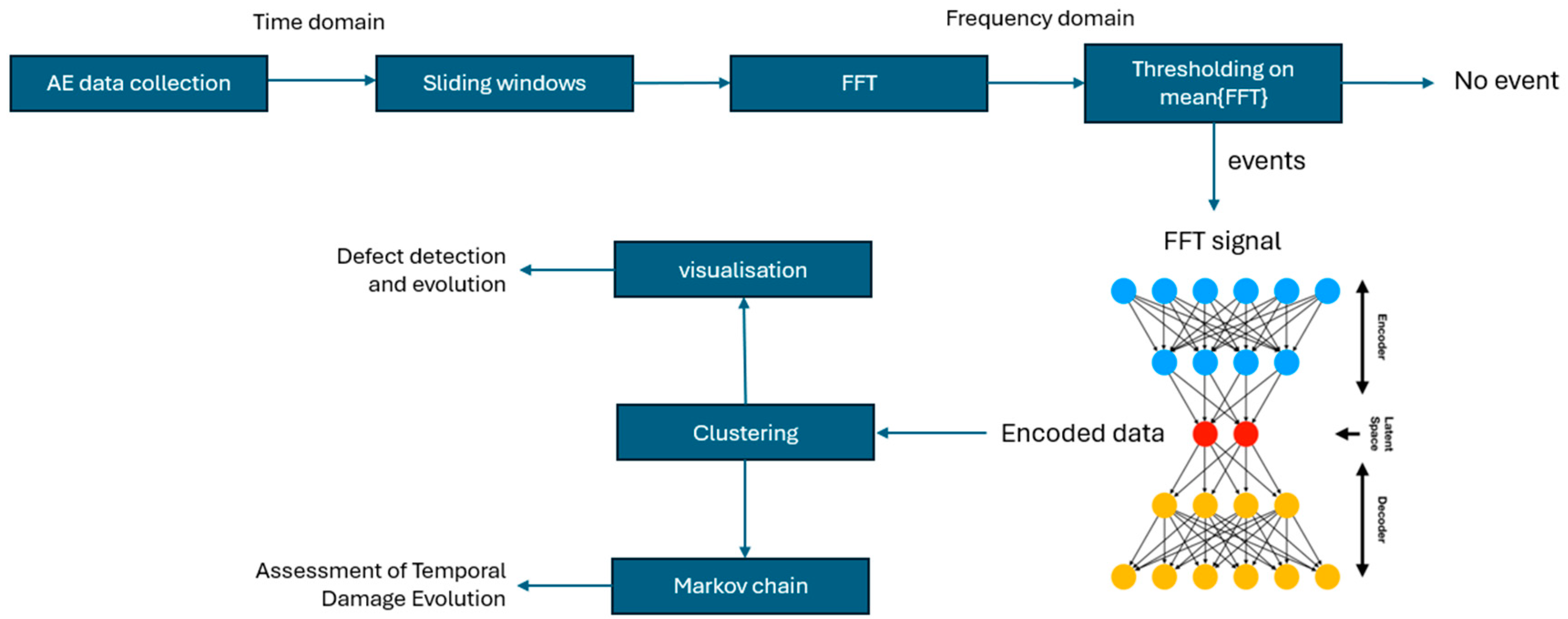
Figure 2.
Sensor positions for the tensile test (left) and 3-point bend (right).
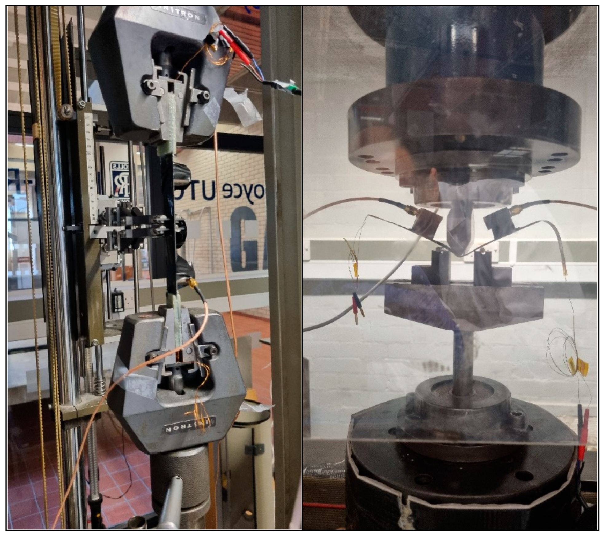
Figure 3.
Raw acoustic data captured from a sample strip in the 3-point bending machine.
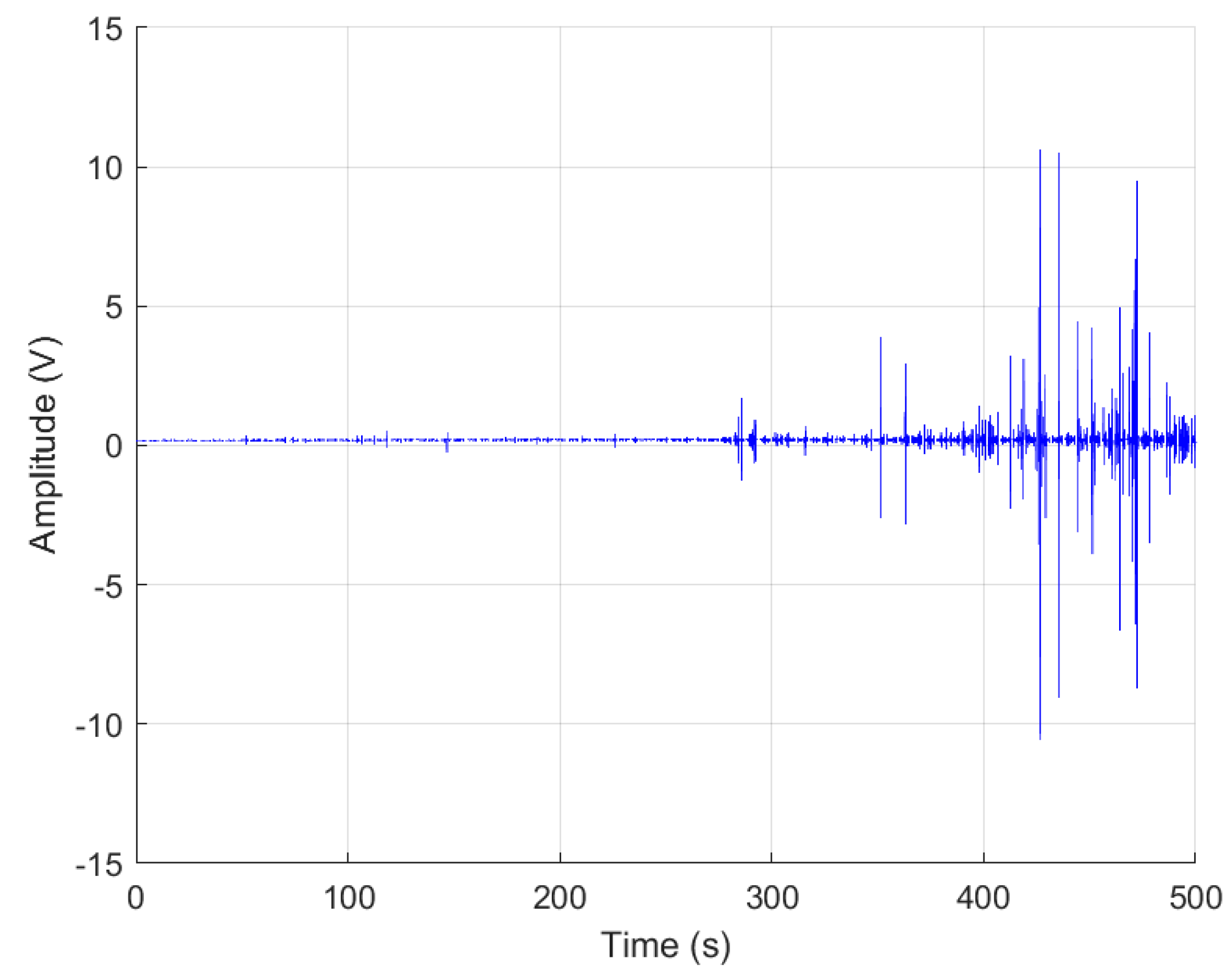
Figure 5.
Time- and frequency-domain of AE signals: a) and b) data with a detected AE event, c) and d) data without a detected AE event.
Figure 5.
Time- and frequency-domain of AE signals: a) and b) data with a detected AE event, c) and d) data without a detected AE event.
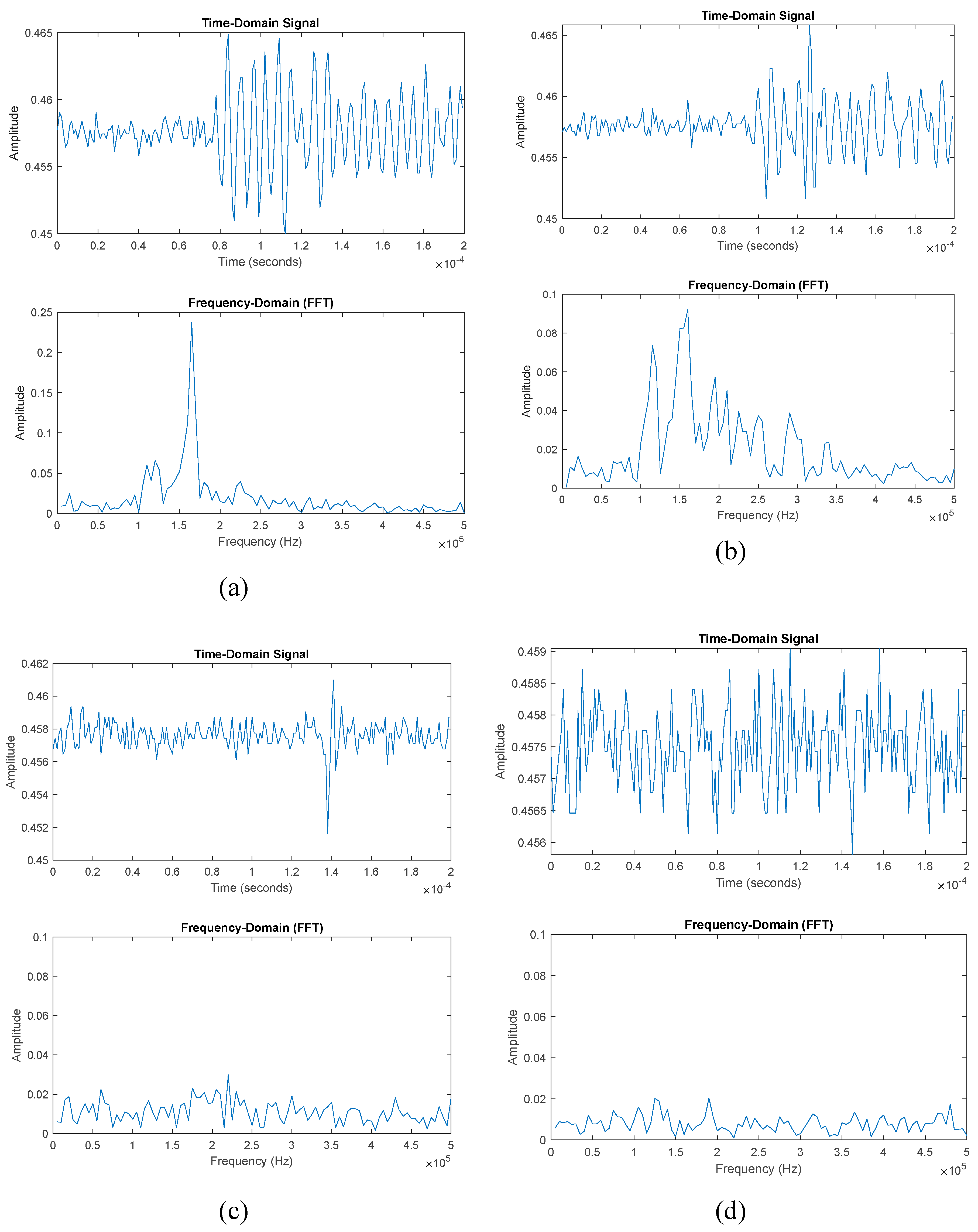
Figure 6.
Thresholding on the frequency domain for detection of events (example from lab experiment T04).
Figure 6.
Thresholding on the frequency domain for detection of events (example from lab experiment T04).
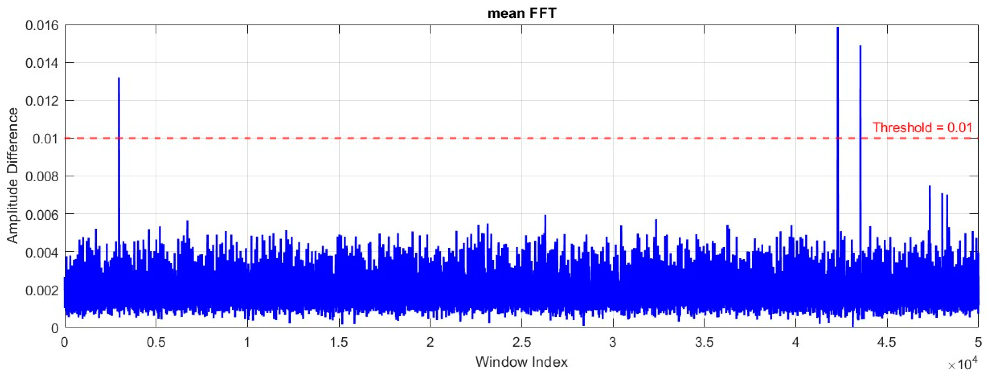
Figure 7.
Examples of reconstructed and original FFT signals.
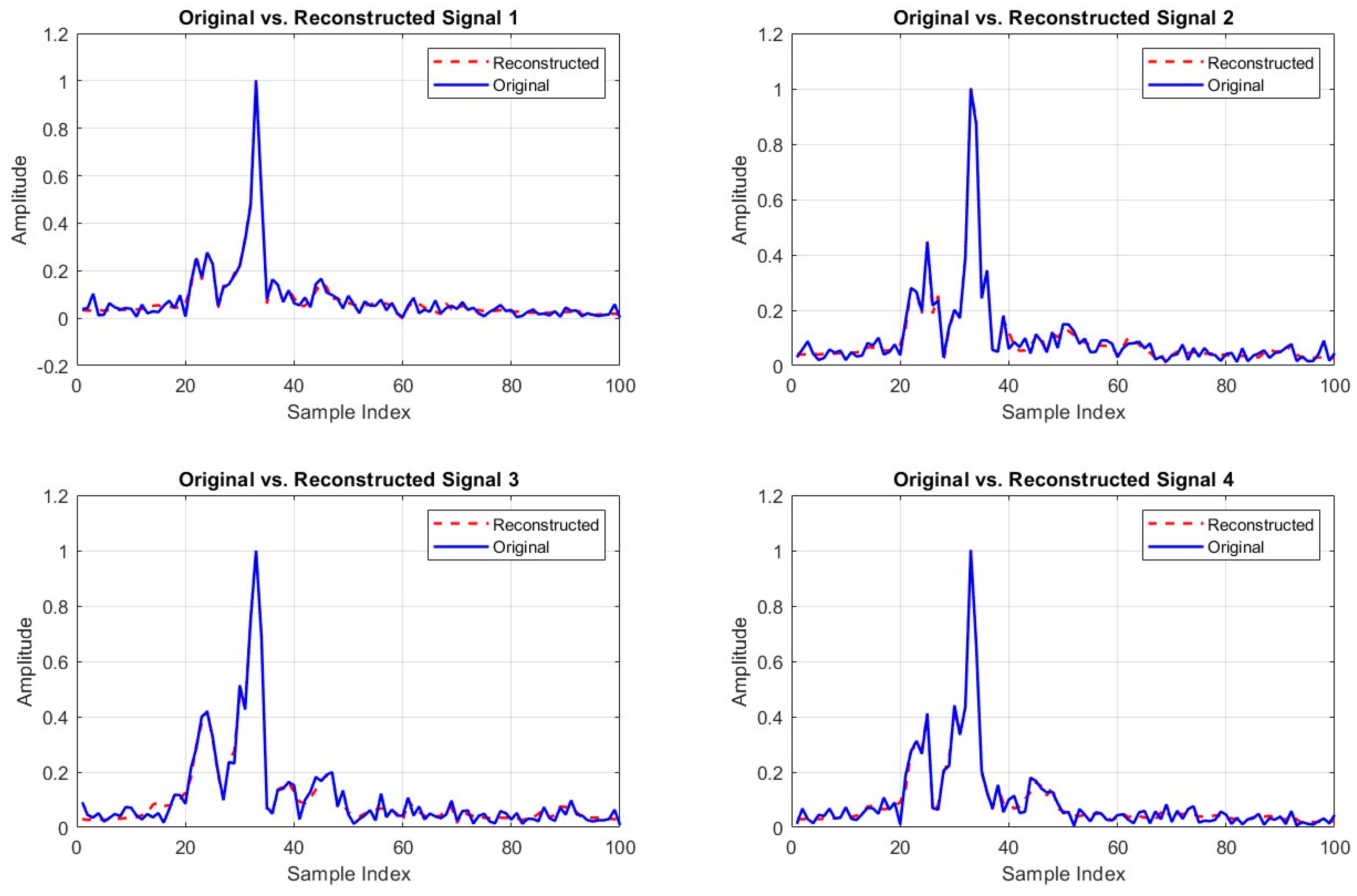
Figure 8.
Analysis of the mean frequency content of two clusters over time. The top plot shows the evolution of the mean frequency content for Cluster 1 and Cluster 2 with accumulated mean frequency curves. The bottom plots display the normalised amplitude of the mean frequency signals for Cluster 1 (left) and Cluster 2 (right), highlighting distinct peaks at specific frequencies within each cluster (results for lab experiment T04).
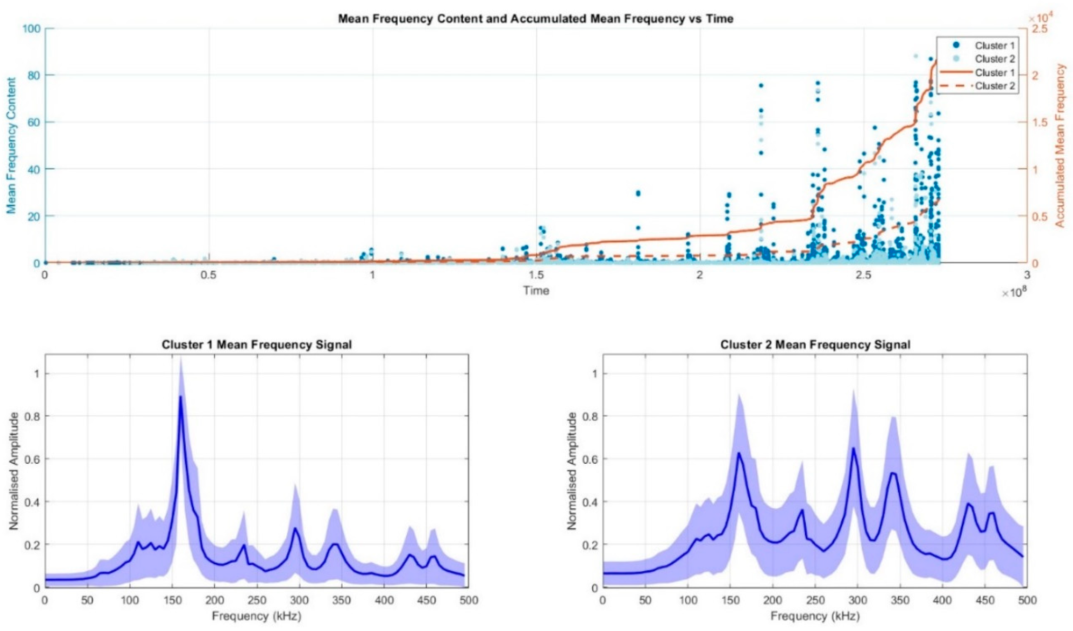
Figure 9.
State Transition Diagram (Markov Chain) representing the probability of transitioning between two clusters. The diagram shows self-transition probabilities for Cluster 1 and Cluster 2, as well as the transition probabilities between the two clusters. The width of the arrows is proportional to the transition probabilities, with values indicated along each transition path.
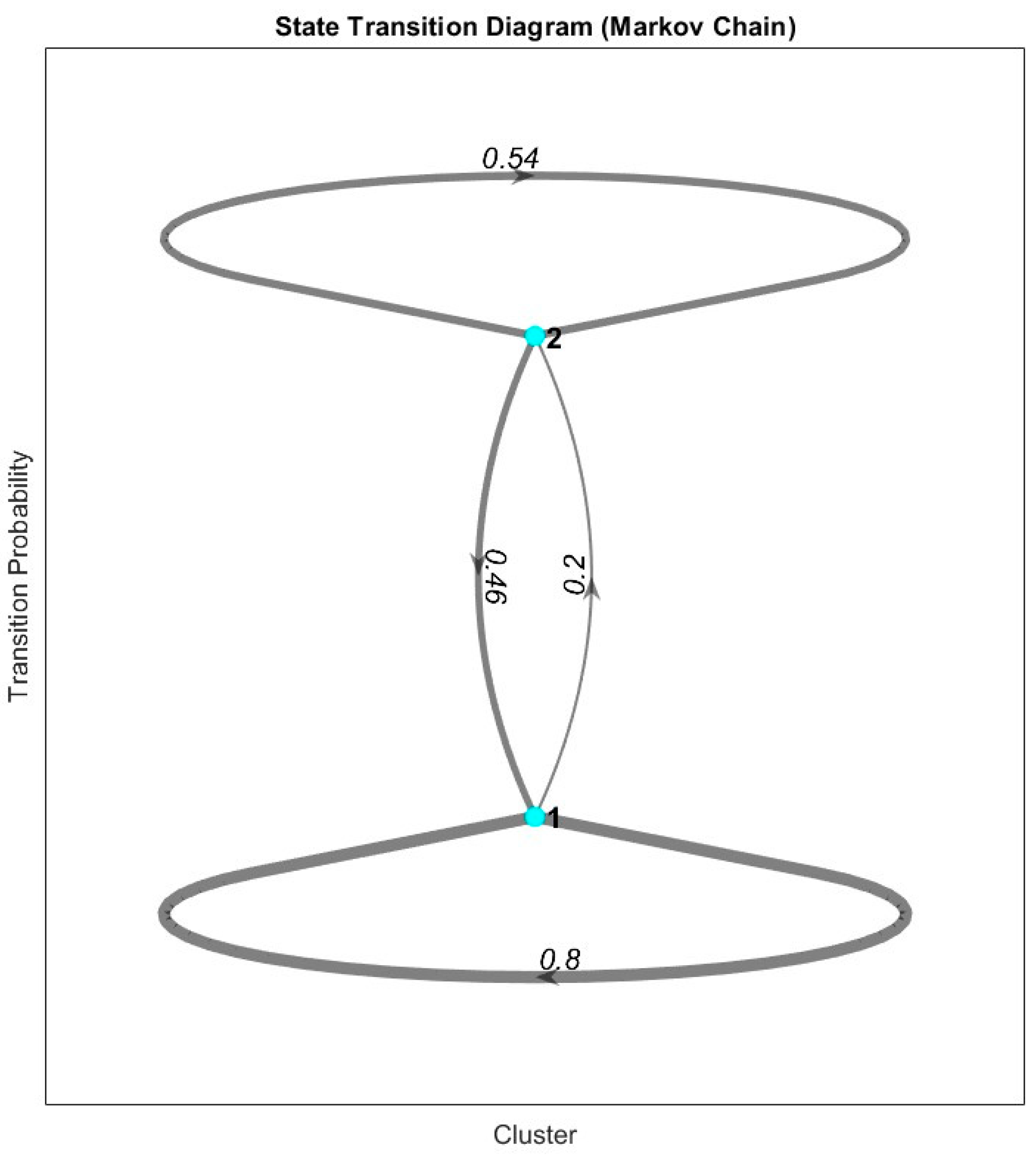
Table 2.
Hyperparameters and performance of the autoencoders.
| Hyperparameter | Value |
| L2 Weight Regularisation | 4.0959e-05 |
| Sparsity Regularisation | 0.26843 |
| Sparsity Proportion | 0.27307 |
| Encoding Dimension | 76 |
| Maximum Epochs | 293 |
| L2 Weight Regularisation | 4.0959e-05 |
| Metric | Performance |
| Global Mean Squared Error (MSE) | 0.0017259 |
| Global R-squared (R²) | 0.94774 |
Table 3.
Comparative analysis based on silhouette scores.
| Number of clusters | silhouette score |
|---|---|
| 2 | 0.3687 |
| 3 | 0.1680 |
| 4 | 0.0689 |
| 5 | 0.0851 |
Disclaimer/Publisher’s Note: The statements, opinions and data contained in all publications are solely those of the individual author(s) and contributor(s) and not of MDPI and/or the editor(s). MDPI and/or the editor(s) disclaim responsibility for any injury to people or property resulting from any ideas, methods, instructions or products referred to in the content. |
© 2024 by the authors. Licensee MDPI, Basel, Switzerland. This article is an open access article distributed under the terms and conditions of the Creative Commons Attribution (CC BY) license (http://creativecommons.org/licenses/by/4.0/).
Copyright: This open access article is published under a Creative Commons CC BY 4.0 license, which permit the free download, distribution, and reuse, provided that the author and preprint are cited in any reuse.


