1. Introduction
This work is motivated by an attempt to describe the fluid behavior of a flat plate in flapping mode. Experimental visualization and numerical calculations are used to fulfill this purpose. The experimental and the numerical calculations are qualitatively compared using both approaches. Then, the velocity field and the dynamic pressure obtained with numerical calculations are analyzed using the Proper Orthogonal Decomposition (POD) to find the main properties of the complex fluid flow.
Flapping motion is a common phenomenon in various engineering applications, such as nuclear safety systems [
1], energy harvesting devices [
2], pendulous behavior in water oil fields [
3], and the design of biomimetic micro air vehicles [
4,
5,
6,
7,
8,
9,
10,
11,
12,
13,
14,
15,
16,
17]. In this last application, much research has been done on visualization and measurements to study these prototypes and understand insect flight physics [
4,
5]. The flow around a flapping plate is usually studied using the PIV technique [
6,
7,
8,
9,
10,
11,
12,
13,
14]. Few works have been reported using the Schlieren method to analyze the flow around a flapping plate [
15,
16,
17]. The Schlieren technique detects refractive index variations in a fluid flow, allowing us to observe its state. The Schlieren method offers some advantages compared with other techniques: it is easy to implement, uses conventional sources for its operation, has variable sensitivity, and is a low-cost method [
18]. In [
15,
16], using the Schlieren method, a solvent was put on the insect wings to visualize the behavior of fluid flow around them. Also, in [
17], a sophisticated temperature gradient generator was developed to study the flapping wings of houseflies. In the same way, in this work, we use the classical Schlieren system as an alternative to visualize the flow behavior of a flapping plate in quasi-quiescent fluid.
On the other hand, the POD method was used to extract organized structures in turbulent flows [
19]. The method obtains an orthonormal basis function from an ensemble of data. The most important property of the POD method is its optimality, in the sense that it provides the most efficient way of capturing the dominant features of an infinite-dimensional process with only a few POD modes. For this reason, the POD method has been extensively used to examine turbulent flows, particularly in the analysis of Direct Numerical Simulation (DNS) data [
20,
21,
22,
23,
24]. The POD analysis has also been used in flapping wing studies, for example, in wing wake interaction [
25,
26], flapping hovering wings [
27], vortex identification and evolution [
28,
29,
30,
31], and in combination with Galerkin projection [
32].
This work used the time-resolved Schlieren technique to visualize a plate (plate or wing) flapping motion. A programmable chilling/heating plate generates a temperature gradient (quasi-quiescent fluid flow) to record the Schlieren images of the flapping wing. The unsteady fluid flow yielded by the flapping wing is spatially and temporally resolved using a fast camera. A numerical calculation is realized using the same condition as its experimental counterpart. The velocity and dynamic pressure field obtained with the numerical calculation are used to find the main component of unstable fluid flow using the POD method.
2. Theoretical Background
2.1. Numerical Model to Simulate the Flapping Movement
ANSYS Fluent software solved the fluid flow modeling of the flapping plate.
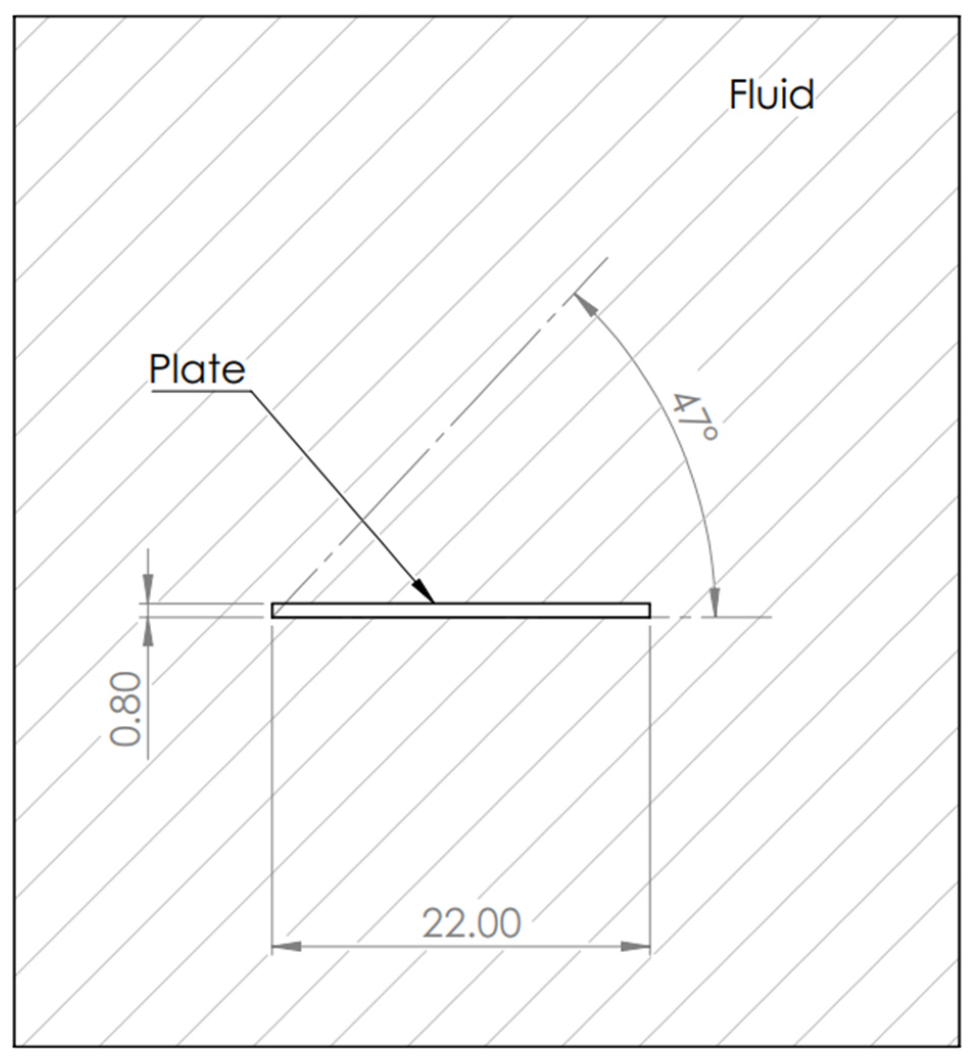
Figure 1 shows a schematic view of the 2D problem to resolve, which we analyzed in the present study. A triangular element was used to generate the mesh to examine the fluid; body sizing, inflations, and edge sizing are used in the meshing with mesh refinements in the plate to capture boundary layer effects better. The number of nodes was 107180 and 208375 elements. The flapping plate has a length of 0.022m and a width of 0.0195m and is subjected to flap frequencies of 10 Hz, 30 Hz, and 40 Hz. Its maximum flapping amplitude is 47°, with an upper stroke of 47° and a lower stroke of 0° (see
Figure 1), and it has a zero-pitch angle. The plate flaps in steady-state fluid at a temperature of 288.16 °K, with a viscosity of 1.7894e-05 kg/(m s) and an air density of 1.225 kg/m3.
2.2. Brief Remarks on the POD Method
Before proceeding, some remarks on notation are introduced. We will use the symbols
x and
y for axial and transverse directions;
x represents a vector. The corresponding velocity components are
u and
v. The dynamic pressure is denoted as
p. Therefore,
ui can be
u,
v, or
p. Any time variable describing a parameter of a flow, such as a velocity or pressure, can be defined as a composition of an average and a random component, as given below:
where
and
are the mean and the random component of any time variable. Thus, the eigenfunctions (or POD modes) are calculated for the random flow component;
.
The proper orthogonal consists of finding a series of POD modes from a data set [
19,
20,
21]. The core of the method is to solve the integral eigenvalue equation:
where
D is the two-dimensional domain of the velocity or pressure field and the kernel,
R, is the average autocorrelation function. The solution of Equation (2) represents a set
n of basis functions with special properties attractive to derive dynamical equations via Galerkin projection.
The eigenfunctions form an orthogonal system, which can be normalized as:
where
δmn is the Kronecker delta symbol. The system
n is complete because the function field
ui represents an expansion of orthogonal eigenfunctions,
where
ς nis the dot product for
ui and
n. That is,
ς n is the projection of
ui in the direction represented by
n. An important property of eigenfunction
n is that it can be expanded as a linear combination of the instantaneous velocity or pressure fields as:
where, the eigenfunction
possess the properties of the velocity or pressure field.
In this work, the data used are velocity and pressure field realizations of 90×120 vectors corresponding to a vector length of 10800. The corresponding autocorrelation matrix has dimensions of 10800 × 10800. The solution to the eigenvalue problem for such a large matrix is cumbersome and time-consuming with the current computers. In [
20] proposed an equivalent approach to overcome this difficulty in which the correlation matrix
R can be expressed as:
Here, M is the number of snapshots (or realizations).
If Equations (2), (5) and (6) are combined, the following equation is obtained:
where
C is an
M ×
M matrix defined as:
In Equation (7), C is a real symmetric matrix with positive real eigenvalues, and Acan be structured in decreasing order of the corresponding eigenvalues λ1 > λ2 > ,…..,λn > 0.
3. Experimental Procedure
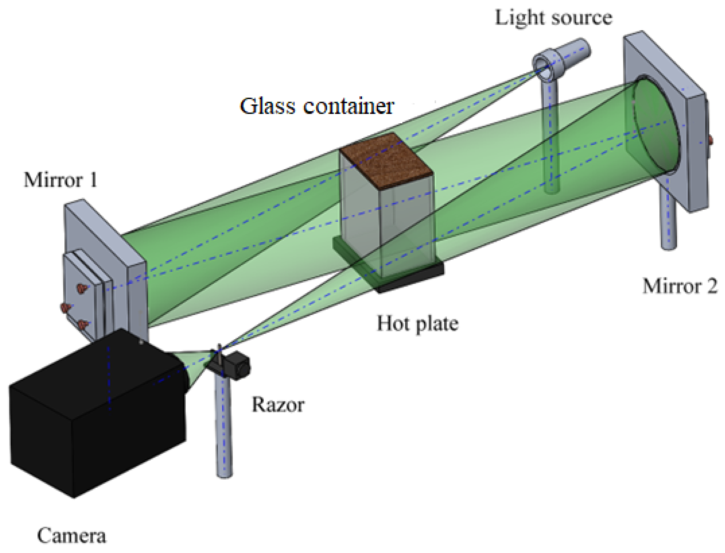
To obtain images of the fluid flow around the flapping mechanism, the Schlieren system shown in
Figure 2 was used. It consists of a white Light-Emitting Diode (LED) source of 3 Watts, two spherical mirrors with a curvature radius of 2 m and a diameter of 0.20 m, a common razor blade, and a high-speed camera MotionPro model Y7 from IDT corporation. 500 images were registered at a frame rate of 5000 Hz. Images were taken with the razor blade in a vertical position to gather more information on the vortex structure formation phenomenon.
The flapping mechanism was constructed using a four-bar linkage mechanism driven by a DC motor with a maximum operating power supply of 5V. The flapping plate’s dimensions are 0.022m and 0.0195m in length and width, respectively. Three fixed flapping frequencies of 10 Hz, 30 Hz, and 40 Hz were studied. The mechanism prototype was placed inside a glass container measuring 0.13×0.09×0.19 m3. The glass container was then placed over a programmable chilling/heating plate provided by Torrey Pines Scientific. The top of the glass container was covered with a wooden board with a slot for securing the flapping mechanism. The temperature set on the surface of the heating plate was 80 °C. The space was sealed, allowing only uniform convection flow generated with direction to the top. The flapping mechanism was placed approximately 0.02 m above the hot plate, which heated the surrounding air to about 40 °C. Reference images were taken without the flapping mechanism in the confined space and at ambient temperature. After placing the mechanism and raising the hot plate temperature, once the working temperature was reached and the flow within the observation area was stable, the mechanism was turned on in each of the three studied frequencies. With the prototype on and after 2 to 3 cycles, 500 Schlieren images were taken. This was repeated for the three mentioned frequencies.
4. Results and Discussion
4.1. Numerical Results
The behavior of the flow field around the flapping plate of each case under analysis can be summarized as follows. A tip vortex is formed at the up and down stroke; these two vortexes roll up over the flapping plate until they stretch and later form a spanwise flow (see
videos LF_S1-10 Hz, MF_S1-30 Hz, and HF_S1-40 Hz, the videos show a flapping cycle of the velocity field overlaid with the dynamic pressure). This behavior is maintained during each cycle of the flapping plate, with the difference that in each case under analysis, the magnitude of the velocity is different, and where the magnitude of the velocity is higher for the flapping plate of 40 Hz.
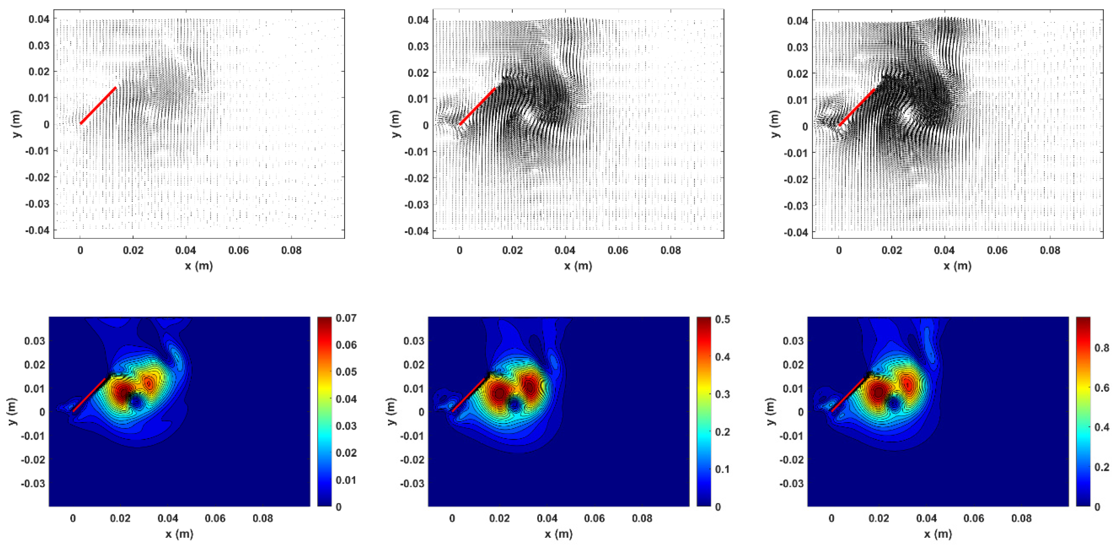
Figure 3 shows the instantaneous velocity and pressure field at the same plate flapping angle (45°) for the three frequencies. In the case of the velocity field, for the three cases, we can note a clockwise rotating vortex (a tip vortex), the main difference being the magnitude of the velocity and the rotation phase of the vortex. Also, a small clockwise vortex is observed at the point of rotation of the flapping plate due to the inherent movement of the point of rotation and initial conditions set to solve the numerical model. The main difference in the pressure fields in each case under study is the value of the pressure. The pressure patterns are similar (not equal), and we can note a drop in the pressure value in the area where the vortex is located.
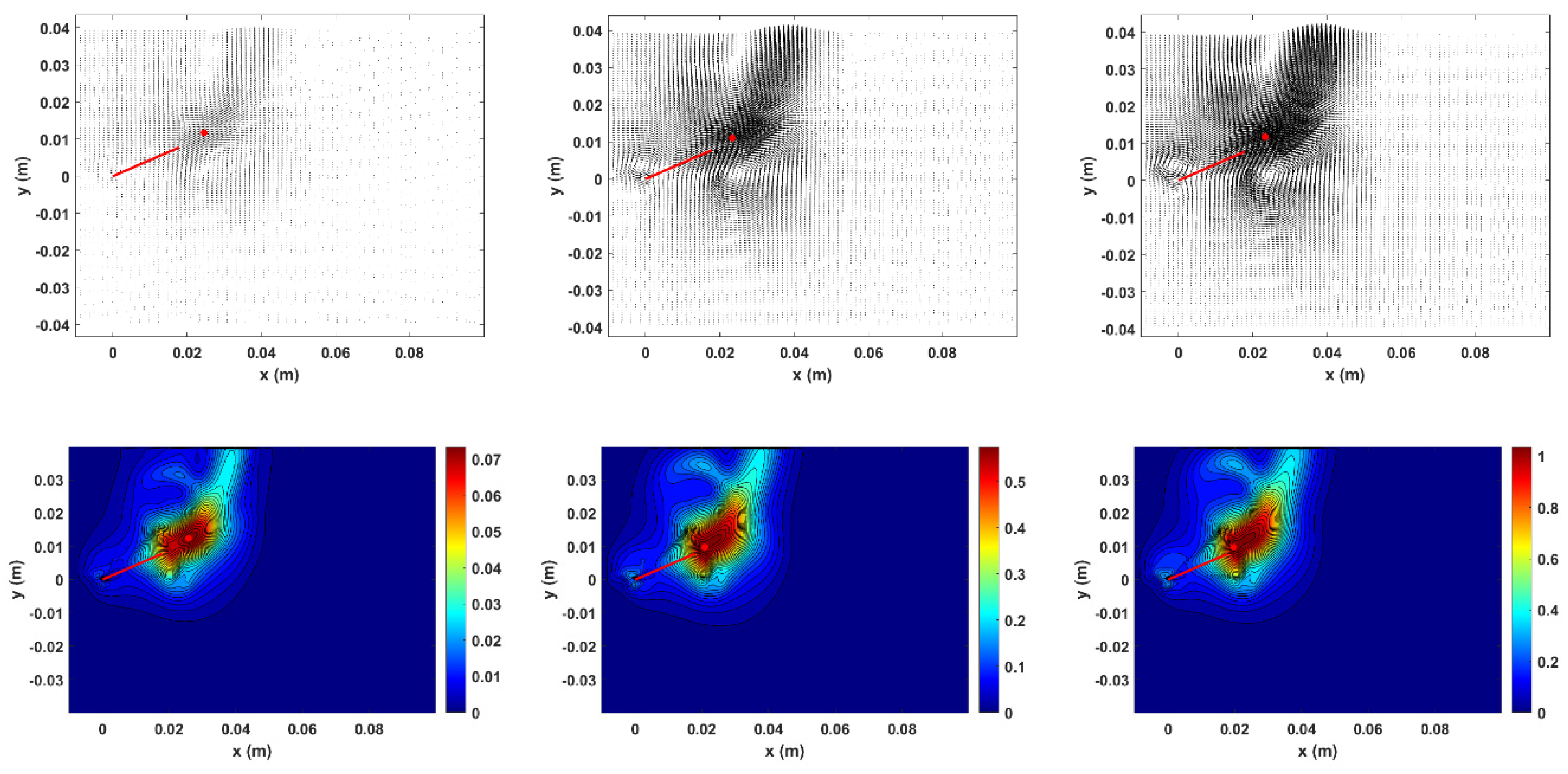
Figure 4 depicts average velocity and pressure fields; the maximum value of the velocity and pressure is indicated with a red solid circle. We can note that this maximum is located almost in the same place for both velocity and pressure, where the up and down stroke vortex merge.
4.2. Experimental Results (Schlieren Images)
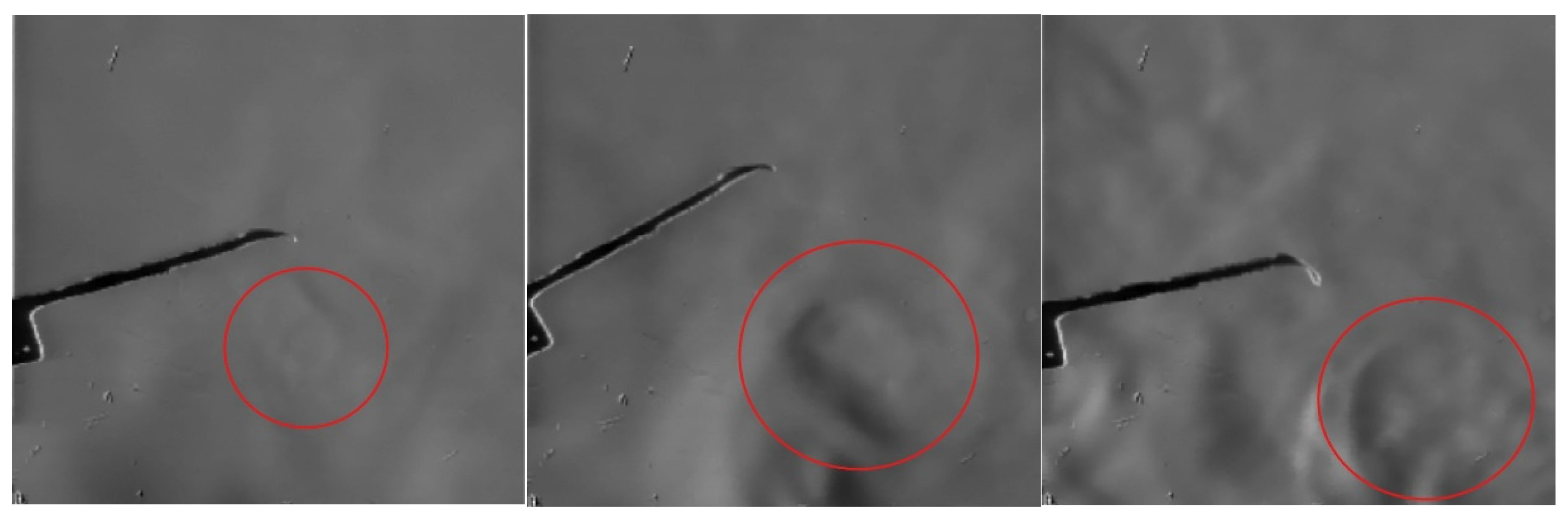
A set of 500 Schlieren images was obtained with a frame rate of 5000 images per second for each plate flapping frequency. Each set of images was obtained after the plate was moved continuously for roughly one second. In this process, depending on the case, the images show unstable flow behavior due to the movement of the plate (see
videos LF_E1-10 Hz, MF_E1-30 Hz, and HF_E1-40 Hz; the videos show a flapping cycle of the plate). These Schlieren images (disturbed) are subtracted from the reference image (undisturbed). After, the section of the image where the airflow disturbed by the plate is located is selected.
We can note that during the up and down strokes of the flapping plate, a tip vortex is formed. However, unlike the simulated results, the vortex is weaker, and its duration is very short.
Figure 5 shows selected Schlieren images from the videos for each case under analysis. In
Figure 5, a red circle indicates the formation of a tip vortex. Due to the velocity, the tip vortex formation is sharper for 30 Hz and 40 Hz because the movement of the plate is at a higher frequency. Then, the movement of the fluid acquires greater velocity, inducing the formation of vortices more easily.
4.3. Qualitative Comparison of Experimental and Numerical Results
The main characteristics of the unsteady flow formed by the flapping plate are maintained in the experimental and numerical cases. In simulated cases, a tip vortex is formed during the up and down stroke during each cycle of the flapping plate. These two vortices merge above the plate to create a spanwise fluid flow. The three cases show the same behavior.
The experimental results show that the tip vortex is clearly created during the upstroke cycle in three cases. However, it is barely noticeable during the downstroke cycle. This may be because a nearly steady air flow occurred under the initial experimental conditions with movement from the bottom to the top of the glass container, preventing the vortex formation during the downstroke cycle. On the other hand, the movement of the flapping plate causes the airflow to become turbulent inside the glass container, making the formation of vortices difficult and their duration very short. Despite this, the fluid’s dynamic behavior in the experimental and simulated results is in good concordance.
4.4. POD Method Results
The POD method is applied to the random component of the velocity and pressure flow fields (see Equation (1)). Then, the average velocity and pressure of the flow are obtained using 556 instantaneous velocity and pressure fields (see
Figure 4). The random component of the velocity and pressure is obtained by subtracting the average of the variable from each instantaneous flow variable. Equation (7) is used to calculate eigenfunctions and eigenvalues.
4.4.1. Energy Distribution
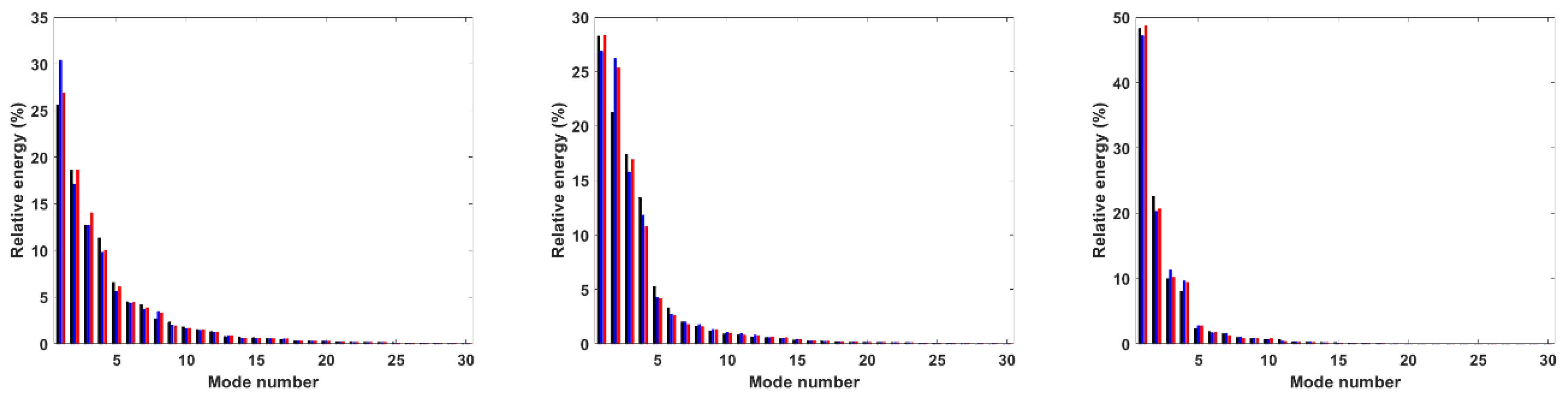
The energy associated with different POD modes is contained in their corresponding eigenvalue (
λ). In Equation (7), the eigenvalues can be ordered from higher to the lower value. Then, the relative value of each eigenvalue can be determined as:
Figure 6 represents the relative energy of the pressure,
u-velocity, and
v-velocity of the first 30 POD modes. The black, blue, and red colors used in bar graphs represent the flapping plate of 10 Hz, 30 Hz, and 40 Hz frequencies used in the experiments and simulations. The results show that the energy associated with the POD modes of the pressure is distributed homogeneously. On the contrary, the
u-velocity shows four dominant POD modes, and the
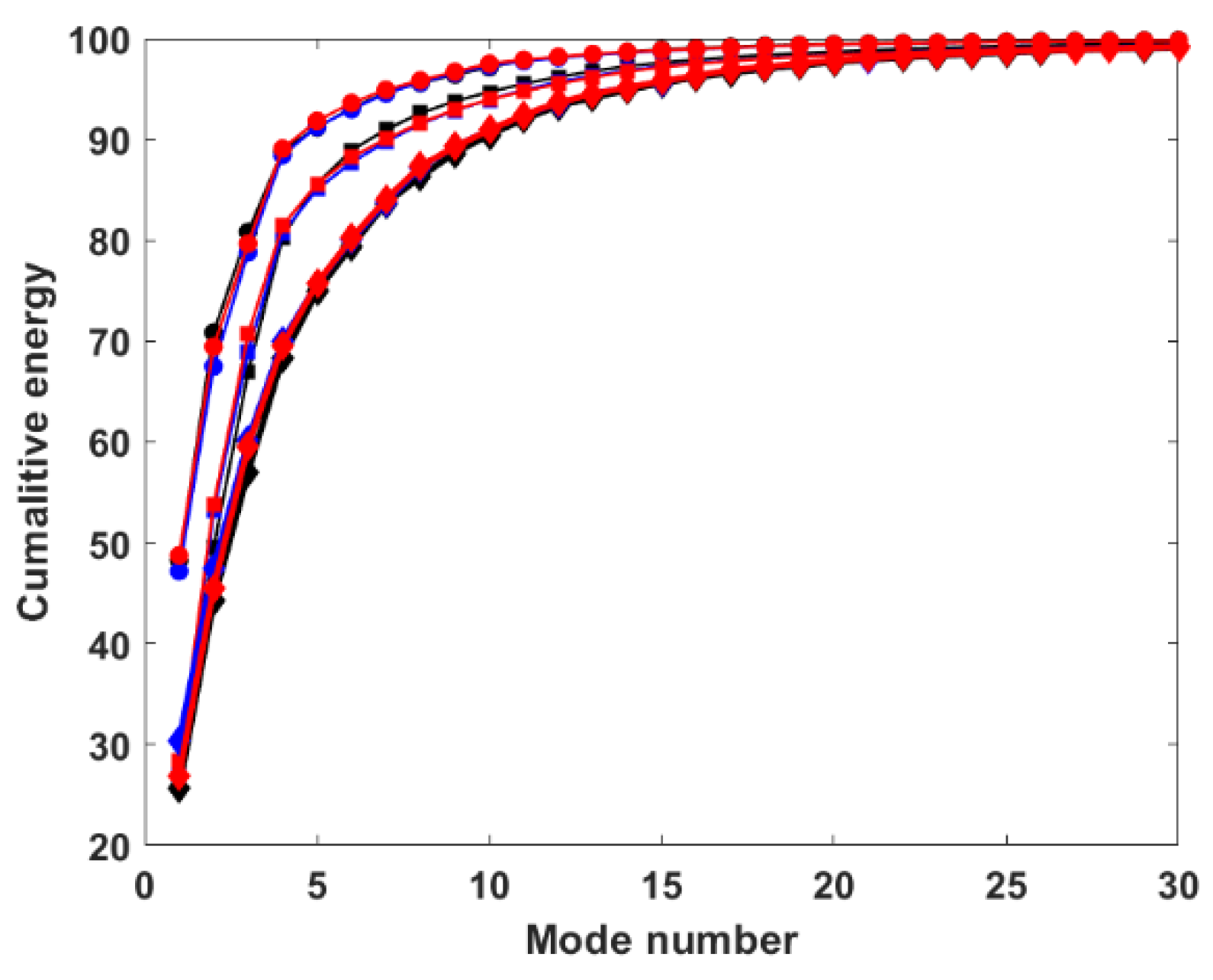
v-velocity shows an energetic dominant POD mode. The cumulative energy is represented in
Figure 7. We note that 90% of the energy is accumulated in 10, 7, and 4 POD modes for the pressure,
v-velocity, and
u-velocity, respectively. On the other hand, the energy associated with each POD mode related to the frequency of the flapping plate does not show a specific trend.
4.4.2. POD Mode Shapes
The characteristics of the POD modes are analyzed for each flapping plate frequency.
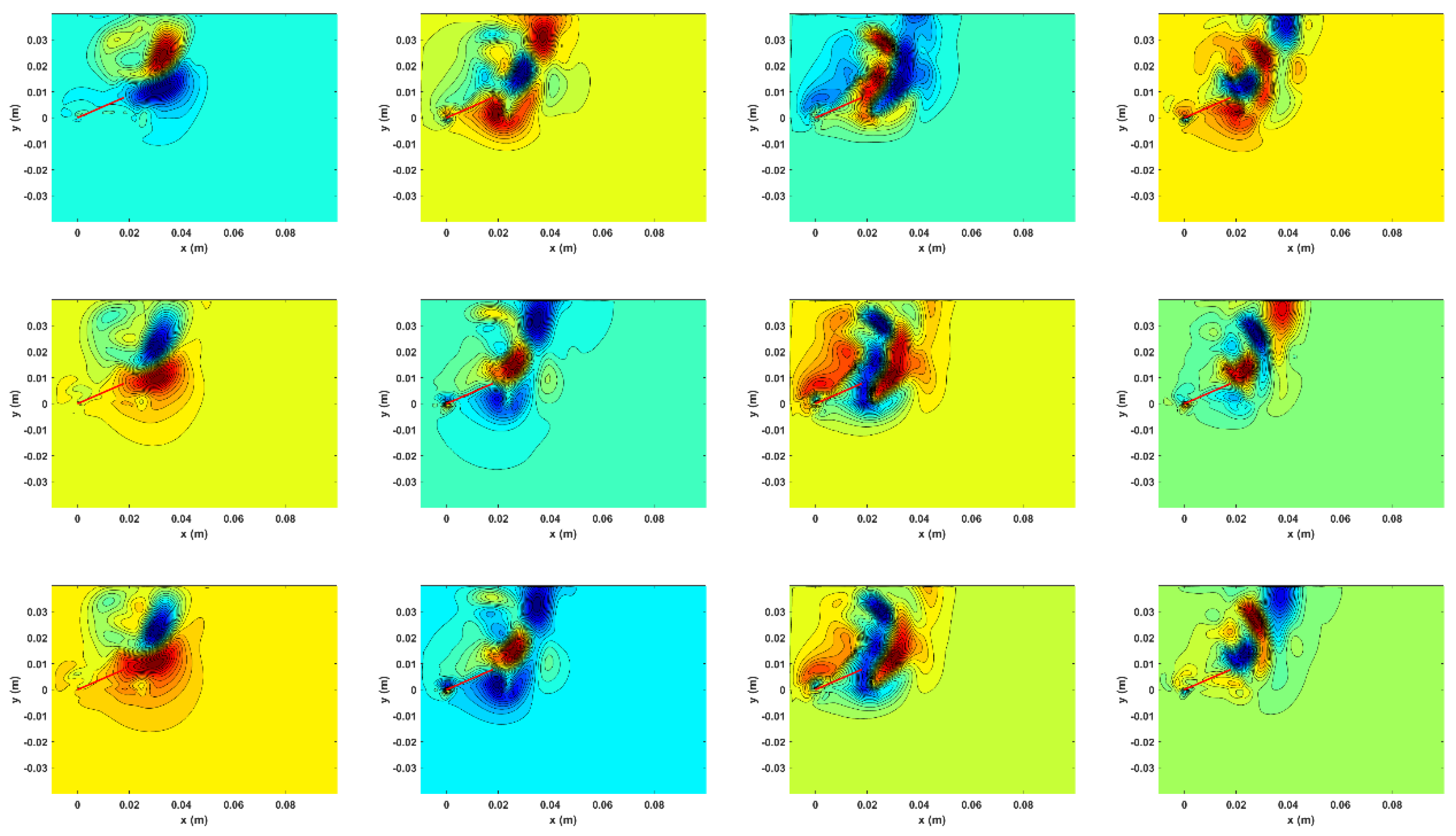
Figure 8 and
Figure 9 represent the first four POD modes for the pressure and velocity fields, respectively. The pressure POD modes shown as color contours represent positive (red) and negative (blue) values. The three POD modes of the flapping plate at 10 Hz are similar in shape to the 30 Hz and 40 Hz but with red and blue color inverted. However, the first three POD modes of these last two flapping frequencies are similar. The fourth POD mode in the three flapping plate frequency cases is different. In general, these red and blue color values correspond to vortical structures in the velocity flow field.
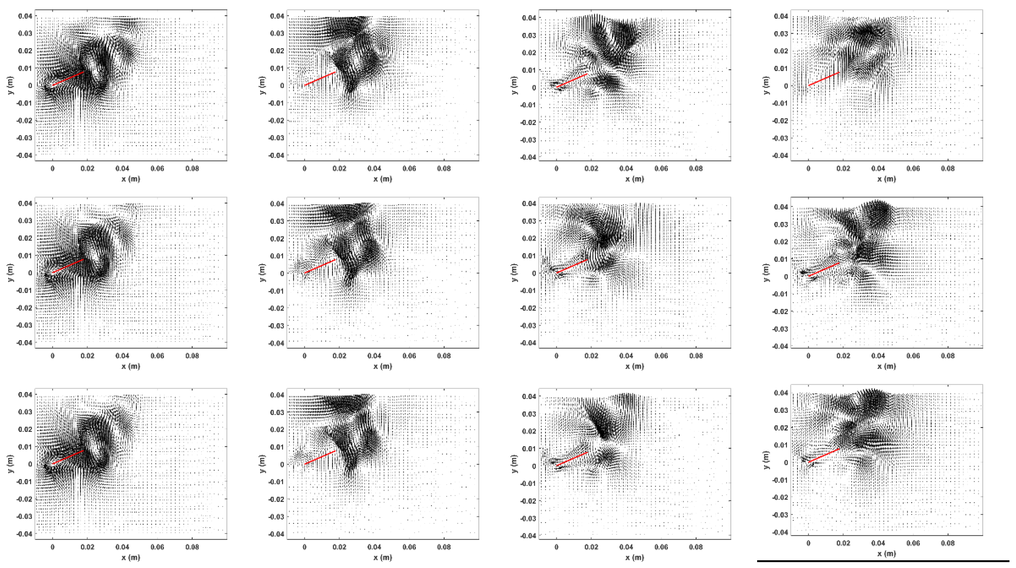
On the other hand, the first two POD modes of the velocity field are similar in shape for each flapping plate frequency under study. In the first POD mode, two main vortical structures are observed at the end of the flapping plate: a large counterclockwise and a small clockwise stretched vortical structure. Also, at the point of rotation of the plate, a clockwise vortex is observed. In the next POD mode, a couple of vortical structures are also observed at the end of the plate. However, the third and fourth POD modes are different for each frequency under analysis; these do not have a specific form.
4.4.3. Reconstruction of Velocity Fields
Reconstructing an instantaneous velocity field will give us an idea of the contribution of each POD mode to that field (see Equation (4)).
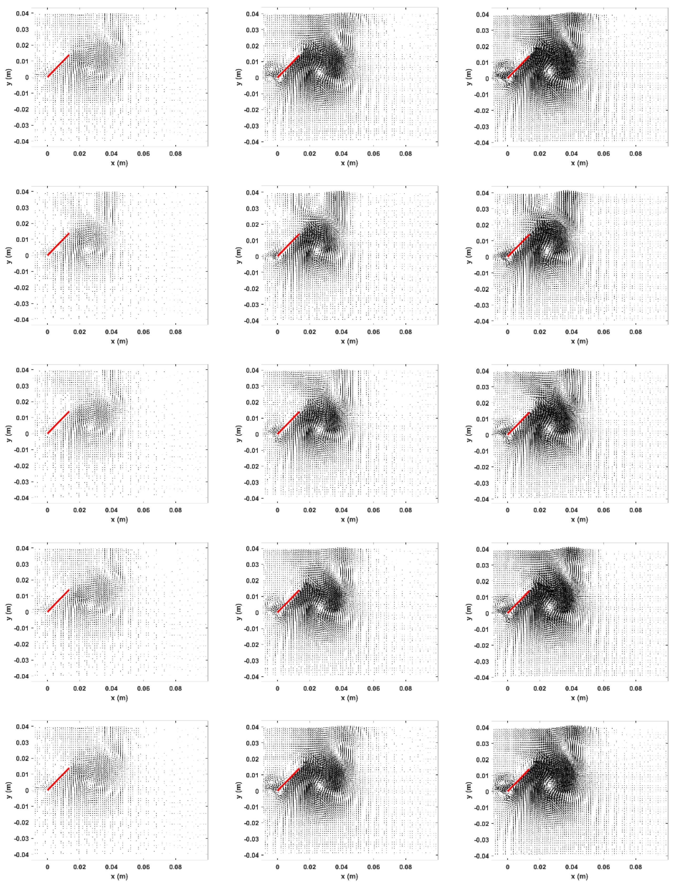
Figure 10 shows the reconstruction with one, five, ten, and fifty POD modes of the instantaneous velocity field of
Figure 3. Using the first POD mode in the reconstruction, the big tip vortex in the velocity field is practically reconstructed. So, we can deduce that the first POD mode is related to the tip vortex formed in this phenomenon. The following POD modes add to the reconstruction of the velocity field fine details. The velocity field reconstruction for the other two frequencies shows the same behavior as the first one.
Table 1 depicts the evolution of the relative error during the velocity field reconstruction. The relative error does not show a specific trend between each flapping frequency. However, for ten POD modes used for reconstruction, the relative error is below 8%, and the velocity field of each case under study contains 90 % of the system’s total energy (data), which is adequate for representing a low-dimensional system model.
5. Final Remarks on This Study
Finally, some observations can be resumed in the following four points:
- -
The initial conditions for the velocity field calculation are for a fluid at rest. However, the fluid (air) is almost at rest in the experimental case. On the other hand, the plate used in the simulated case is rigid, but in the experiment, it is somewhat flexible. Despite these variations in both approaches, the behavior of the fluid during the flapping plate is consistent in the experimental and simulated cases.
- -
The Schlieren method in this work offers advantages over other techniques, such as PIV. It avoids particles in the flow, high-power lasers, and complicated optical array alignments.
- -
The numerical data of the dynamic pressure show that despite being a plate in flapping mode, there are no apparent signs of wing lift in any of the cases analyzed.
- -
The POD method allowed us to decompose the velocity fields of the three cases analyzed into the main characteristics of the unsteady flow under study. The first POD mode is related to the tip vortex that forms during the plate’s up and down strokes.
6. Conclusions
In this work, we present the Schlieren method to study the flapping motion of a rigid plate. The same phenomenon is also simulated using ANSYS Fluent software. Both experimental and simulated results show high qualitative similarities. The POD method is applied to velocity fields obtained from numerical simulations. These results show that the first four POD modes contain high energy of the system’s total energy. On the other hand, the shapes of the first two POD modes are almost equal for the three frequencies of the flapping plate under study. Clearly, it is the same phenomenon but for different frequency plate movements. The difference in POD mode shapes due to plate flapping frequency is probably found from the third POD mode onwards, as shown in the results. This study is preliminary. In future works, we will focus on quantitatively comparing the velocity fields of the unsteady flow generated by a flapping plate. The analysis also will be extended to different up and down stroke angles of the plate.
Supplementary Materials
The following supporting information can be downloaded at the website of this paper posted on Preprints.org. Videos: LF_S1-10 Hz, MF_S1-30 Hz, HF_S1-40 Hz, LF_E1-10 Hz, MF_E1-30 Hz, and HF_E1-40 Hz. S-Simulation, E-Experimental.
Author Contributions
Conceptualization, D.M.H; methodology, C.E.H.M., J.M.G.R, and D.M.H.; software, C.E.H.M. and D.M.H.; validation, C.E.H.M., J.M.G.R., and D.M.H..; formal analysis, D.M.H. and A.M.G.; investigation, D.M.H. and A.M.G.; resources D.M.H. and A.M.G; writing—original draft preparation, D.M.H. and J.M.G.R.; writing—review and editing, D.M.H. and A.M.G.; visualization D.M.H. and A.M.G; supervision, D.M.H.; funding acquisition, D.M.H. All authors have read and agreed to the published version of the manuscript.
Funding
This research received no external funding.
Data Availability Statement
Data underlying the results presented in this article are not publicly
available but may be available from the corresponding authors upon reasonable request.
Acknowledgments
The authors gratefully acknowledge (CONAHCYT) through different projects and scholarships.
Conflicts of Interest
The authors declare no conflicts of interest.
References
- Wang, H.; Lu, C.; Qu, W.; Xiong, J. Experimental investigation on flow field around a flapping plate with single degree of freedom. Nucl. Eng. Technol. 2023, 55, 1999–2010. [CrossRef]
- Zhu, H.; Gao, Y. Vortex induced vibration response and energy harvesting of a marine riser attached by a free-to-rotate impeller. Energy 2017, 134, 532–544. [CrossRef]
- Zhu, Q. Energy harvesting by a purely passive flapping foil from shear flows. J. Fluids Struct. 2012, 34, 157–169. [CrossRef]
- Triantafyllou, M.; Techet, A.; Hover, F. Review of Experimental Work in Biomimetic Foils. IEEE J. Ocean. Eng. 2004, 29, 585–594. [CrossRef]
- Bomphrey, R.J. Insects in flight: direct visualization and flow measurements. Bioinspiration Biomimetics 2006, 1, S1–S9. [CrossRef]
- Toomey, J.; Eldredge, J.D. Numerical and experimental study of the fluid dynamics of a flapping wing with low order flexibility. Phys. Fluids 2008, 20. [CrossRef]
- Fernandes, A.; Mirzaeisefat, S. Flow induced fluttering of a hinged vertical flat plate. Ocean Eng. 2015, 95, 134–142. [CrossRef]
- Altshuler, D.L.; Princevac, M.; Pan, H.; Lozano, J. Wake patterns of the wings and tail of hovering hummingbirds. Exp. Fluids 2008, 46, 835–846. [CrossRef]
- Bomphrey, R.J.; Lawson, N.J.; Taylor, G.K.; Thomas, A.L.R. Application of digital particle image velocimetry to insect aerodynamics: measurement of the leading-edge vortex and near wake of a Hawkmoth. Exp. Fluids 2006, 40, 546–554. [CrossRef]
- Warrick, D.R.; Tobalske, B.W.; Powers, D.R. Aerodynamics of the hovering hummingbird. Nature 2005, 435, 1094–1097. [CrossRef]
- Johansson, L. C.; Engel, L.; Kelbert, C.; Heerenbrink, S. A.; Hedenstrm, M. K. Multiple leading edge vortices of unexpected strength in freely flying hawkmoth. Scientific Report, 2013, 3, 3264. [CrossRef]
- Young, J.; Walker, S.M.; Bomphrey, R.J.; Taylor, G.K.; Thomas, A.L.R. Details of Insect Wing Design and Deformation Enhance Aerodynamic Function and Flight Efficiency. Science 2009, 325, 1549–1552. [CrossRef]
- Lehmann, F.-O.; Wang, H.; Engels, T. Vortex trapping recaptures energy in flying fruit flies. Sci. Rep. 2021, 11, 1–7. [CrossRef]
- Bomphrey, R.J.; Nakata, T.; Phillips, N.; Walker, S.M. Smart wing rotation and trailing-edge vortices enable high frequency mosquito flight. Nature 2017, 544, 92–95. [CrossRef]
- Liu, Y.; Roll, J.; Van Kooten, S.; Deng, X. Schlieren photography on freely flying hawkmoth. Biol. Lett. 2018, 14, 20180198. [CrossRef]
- Zeng, Z.; Ye, Y.; Jiang, H.; Jiang, J.; Wang, Z.; Yuan, S.; Deng, J. Visualization of Vortices Generated by Flapping Wing Device by Schlieren Method. J. Physics: Conf. Ser. 2021, 1985, 012023. [CrossRef]
- Liu, Y.; Lozano, A.D. Liu, Y.; Lozano, A.D. Investigate the Wake Flow on Houseflies with Particle-Tracking-Velocimetry and Schlieren Photography. J. Bionic Eng. 2022, 20, 656–667. [CrossRef]
- Settles, G. S. Schlieren and Shadowgraph Technique. Springer, 2001.
- Lumley, L. The structure of inhomogeneous turbulent flows. In atmospheric turbulence and Radio wave propagations. (Yaglom A. M.; Tatarsky V. I., editors) Nauka, 1967.
- Sirovich,L. Turbulence and the dynamics of coherents structures. Q. Appl. Math. 1987, 45, 561.
- Berkooz, G.; Holmes, P.; Lumley, J. L. The proper orthogonal decomposition in the analysis of turbulent flows. Ann. Rev. Fluid Mech. 1993, 25, 539.
- Rempfer, D. Investigations of boundary layer transition via Galerkin projections on empirical eigenfunctions. Phys. Fluids 1996, 8, 175–188. [CrossRef]
- Rajaee, M.; Karlsson, S.K.F.; Sirovich, L. Low-dimensional description of free-shear-flow coherent structures and their dynamical behaviour. J. Fluid Mech. 1994, 258, 1–29. [CrossRef]
- Rowley, C. W.; Colonius T.; Murray, R. POD based models of self-sustained oscillations in the flow past an open cavity. June 2000, AIAA Paper 2000-1969. [CrossRef]
- Liang, Z.; Dong, H.; Wan, H.; Beran, P.; Wei, M. Wing-Wake Interaction and its Proper Orthogonal Decomposition. 2010, In 28th AIAA Applied Aerodynamics Conference (p. 5084). [CrossRef]
- Stanford, B.; Albertani, R.; Lacore, D.; Parker, G. Proper Orthogonal Decomposition of Flexible Clap and Fling Elastic Motions via High-Speed Deformation Measurements. Exp. Mech. 2013, 53, 1127–1141. [CrossRef]
- Li, C.; Wang, J.; Dong, H. Proper orthogonal decomposition analysis of flapping hovering wings. In 55th AIAA Aerospace Sciences Meeting. 2017, (p. 0327). [CrossRef]
- Goli, S.; Dammati, S. S.; Roy, A.; Roy, S. Vortex identification and proper orthogonal decomposition of rigid flapping wing. International Journal of Fluid Mechanics Research. 2020, 47(4). [CrossRef]
- Chakraborty, P.; Goli, S.; Roy, A. On dissecting the wakes of flapping wings. Phys. Fluids 2023, 35. [CrossRef]
- Poletti, R.; Calado, A.; Koloszar, L.K.; Degroote, J.; Mendez, M.A. On the unsteady aerodynamics of flapping wings under dynamic hovering kinematics. Phys. Fluids 2024, 36. [CrossRef]
- Goli, S.; Roy, A.; Roy, S.; Imran, I.H. Evolution of Vortex Structures Generated by a Rigid Flapping Wing with a Winglet in Quiescent Water. Proc. Eng. Technol. Innov. 2024, 26, 55–71. [CrossRef]
- Liang, Z.; Dong, H.; Beran, P. POD-Galerkin Projection of Flapping Wings. In 49th AIAA Aerospace Sciences Meeting Including the New Horizons Forum and Aerospace Exposition. 2011, (p. 1051). [CrossRef]
Figure 1.
Schematic view of the problem to model. Units in millimeters.
Figure 1.
Schematic view of the problem to model. Units in millimeters.
Figure 2.
Schlieren optical setup used in this work.
Figure 2.
Schlieren optical setup used in this work.
Figure 3.
Top: Velocity field. Bottom: Dynamic pressure. From left to right: 10 Hz, 30 Hz, and 40 Hz. The graphics show the flapping plate as a thick red line.
Figure 3.
Top: Velocity field. Bottom: Dynamic pressure. From left to right: 10 Hz, 30 Hz, and 40 Hz. The graphics show the flapping plate as a thick red line.
Figure 4.
Top: Average velocity field. Bottom: Average dynamic pressure. From left to right: 10 Hz, 30 Hz, and 40 Hz. The graphics show the flapping plate at an angle of 23.5 ° C as a thick red line.
Figure 4.
Top: Average velocity field. Bottom: Average dynamic pressure. From left to right: 10 Hz, 30 Hz, and 40 Hz. The graphics show the flapping plate at an angle of 23.5 ° C as a thick red line.
Figure 5.
Schlieren images of the flapping plate. From left to right: 10 Hz, 30 Hz and 40 Hz. A tip vortex is selected with a red circle.
Figure 5.
Schlieren images of the flapping plate. From left to right: 10 Hz, 30 Hz and 40 Hz. A tip vortex is selected with a red circle.
Figure 6.
The relative energy of each POD mode. From left to right: pressure, u-velocity, and v-velocity. Black bar: 10 Hz. Blue bar: 30 Hz. Red bar: 40 Hz.
Figure 6.
The relative energy of each POD mode. From left to right: pressure, u-velocity, and v-velocity. Black bar: 10 Hz. Blue bar: 30 Hz. Red bar: 40 Hz.
Figure 7.
Cumulative energy. Square symbol: u-velocity. Circle symbol: v-velocity. Diamond symbol: p-pressure.
Figure 7.
Cumulative energy. Square symbol: u-velocity. Circle symbol: v-velocity. Diamond symbol: p-pressure.
Figure 8.
The first four POD modes of dynamic pressure. From left to right: 1, 2, 3, and 4 POD mode. From top to bottom: 10 Hz, 20 Hz, and 40 Hz.
Figure 8.
The first four POD modes of dynamic pressure. From left to right: 1, 2, 3, and 4 POD mode. From top to bottom: 10 Hz, 20 Hz, and 40 Hz.
Figure 9.
The first four POD modes of velocity field. From left to right: 1, 2, 3, and 4 POD mode. From top to bottom: 10 Hz, 20 Hz, and 40 Hz.
Figure 9.
The first four POD modes of velocity field. From left to right: 1, 2, 3, and 4 POD mode. From top to bottom: 10 Hz, 20 Hz, and 40 Hz.
Figure 10.
Reconstruction of the velocity field. From left to right: 10 Hz, 30 Hz, and 40 Hz. Top row: Original velocity field. The following rows are Reconstruction with 1 POD mode, 5 POD modes, 10 POD modes, and 50 POD modes.
Figure 10.
Reconstruction of the velocity field. From left to right: 10 Hz, 30 Hz, and 40 Hz. Top row: Original velocity field. The following rows are Reconstruction with 1 POD mode, 5 POD modes, 10 POD modes, and 50 POD modes.
Table 1.
Relative error during the reconstruction of a velocity field.
Table 1.
Relative error during the reconstruction of a velocity field.
| Frequency (Hz) |
1 POD Modes |
5 POD Modes |
10 POD Modes |
50 POD Modes |
| 10 |
31.0 |
13.1 |
5.9 |
0.50 |
| 30 |
29.1 |
14.2 |
7.7 |
0.46 |
| 40 |
26.3 |
13.0 |
7.2 |
0.47 |
|
Disclaimer/Publisher’s Note: The statements, opinions and data contained in all publications are solely those of the individual author(s) and contributor(s) and not of MDPI and/or the editor(s). MDPI and/or the editor(s) disclaim responsibility for any injury to people or property resulting from any ideas, methods, instructions or products referred to in the content. |
© 2024 by the authors. Licensee MDPI, Basel, Switzerland. This article is an open access article distributed under the terms and conditions of the Creative Commons Attribution (CC BY) license (http://creativecommons.org/licenses/by/4.0/).