Non-hydrostatic Galerkin Model with Weighted Average Pressure Profile

1. Introduction

In recent decades, the importance of research on wave propagation mechanisms in coastal areas has increased due to many coastal catastrophes, partly increased by rising sea levels.

Depth-integrated models using the Boussinesq-type equations have traditionally been utilized to simulate wave propagation. However, the high-order partial derivative terms in the Boussinesq equations have difficult discretization, cause numerical instabilities, and have a non-negligible computational cost. Additionally, the Boussinesq-type equations arise from the supposition of no rotation and no viscosity.

The shallow water models with non-hydrostatic pressure distribution have shown their capacity for accurately modeling nonlinear and dispersive waves since their introduction by Casulli & Stelling (1998) and Stansby & Zhou (1998). The vertical momentum is considered in these models by introducing a non-hydrostatic pressure term into the Reynolds-averaged Navier–Stokes equations. The non-hydrostatic models for water waves are classified as single-layer models (two-dimensional depth-integrated non-hydrostatic) or multi-layer models (three-dimensional non-hydrostatic), depending on the number of layers in the vertical discretization. Many researchers have demonstrated the capabilities of the non-hydrostatic models for water waves with single or multiple layers in the vertical direction (Stelling & Zijlema, 2003; Zijlema et al., 2005; Zijlema & Stelling, 2008; Zijlema et al., 2011).

Calvo et al. (2021) present a two-dimensional depth-integrated non-hydrostatic model for simulating wave propagation, breaking, and runup in a finite element framework. As with all previous non-hydrostatic models, the model uses a linear vertical profile for the non-hydrostatic pressure. The model is constructed using a combination of continuous and discontinuous Galerkin methods. Good agreements between numerical results and experimental data showed that the model adequately simulates wave motions.

Due to the linearization of the vertical momentum equations, it is well known that the depth-integrated, non-hydrostatic models only apply to the intermediate water depth and weakly nonlinear cases (Bai and Cheung, 2013). Recently, researchers have focused on increasing the order of the non-hydrostatic pressure interpolation from a linear to a quadratic vertical pressure profile, showing improvements in dispersion (Jeschke et al., 2017; Wang et al., 2020 (a), Wang et al., 2020 (b)).

This research aims to develop and validate a new two-dimensional depth-integrated non-hydrostatic model for simulating wave propagation using a linear/quadratic weighted average pressure profile. These objectives are achieved by modifying Calvo et al. (2021) existing non-hydrostatic discontinuous/continuous Galerkin finite element model.

The new model has its dispersive characteristics improved by a linear/quadratic weighted average non-hydrostatic pressure profile, with the additional advantage of using unstructured meshes that easily allow local refinement and complex boundaries. Additionally, the utilization of linear quadrilateral finite elements presents the advantage of requiring fewer nodal variables for a given area than linear triangular finite elements in a discontinuous Galerkin context (e.g., four nodal variables instead of six) and with a higher order of interpolation than their triangular counterparts (e.g., bilinear interpolation). The new method is an interesting alternative for modeling shallow water waves while avoiding the numerical instabilities caused by the higher-order terms in a Boussinesq-type model, as well as the increased computational costs arising from a more significant number of vertical layers in a multi-layer non-hydrostatic model.

2. Description of the Model

The proposed model starts with the non-hydrostatic discontinuous/continuous Galerkin finite element model presented in Calvo et al. (2021). This two-dimensional, depth-integrated non-hydrostatic model can simulate wave propagation, breaking, and runup in a finite element framework.

The non-hydrostatic discontinuous/continuous Galerkin model is constructed using a combination of discontinuous and continuous Galerkin methods, where the depth-integrated non-hydrostatic equations are separated into hydrostatic and non-hydrostatic parts. The hydrostatic part corresponds to the depth-integrated shallow water equations. It is solved with a discontinuous Galerkin finite element method to simulate discontinuous flows, wave breaking, and runup. The non-hydrostatic part resulted in a Poisson-type equation, where the non-hydrostatic pressure was resolved by a continuous Galerkin finite element method for modeling wave propagation and transformation. The model utilizes linear quadrilateral finite elements for horizontal velocities, water surface elevations, and non-hydrostatic pressures that permit local refinement and complex boundaries.

The governing equations in the conservation form for depth-integrated, non-hydrostatic flow in the Cartesian coordinates system ($x$, $y,$ and z) are:

$$\begin{gathered} {\displaystyle \frac{\partial HU}{\partial t}}+{\displaystyle \frac{\partial HUU}{\partial x}}+{\displaystyle \frac{\partial HUV}{\partial y}} \\ =-gH{\displaystyle \frac{\partial \xi }{\partial x}}-{\displaystyle \frac{g{n}^{2}U\sqrt{U^2+V^2}}{H^{\frac{1}{3}}}}-{\displaystyle \frac{H}{2\rho }}{\displaystyle \frac{\partial q_b}{\partial x}}-{\displaystyle \frac{q_b}{2\rho }}{\displaystyle \frac{\partial \left(\xi -h\right)}{\partial x}}[1] \\ {\displaystyle \frac{\partial HV}{\partial t}}+{\displaystyle \frac{\partial HUV}{\partial x}}+{\displaystyle \frac{\partial HVV}{\partial y}} \\ =-gH{\displaystyle \frac{\partial \xi }{\partial y}}-{\displaystyle \frac{g{n}^{2}V\sqrt{U^2+V^2}}{H^{\frac{1}{3}}}}-{\displaystyle \frac{H}{2\rho }}{\displaystyle \frac{\partial q_b}{\partial y}}-{\displaystyle \frac{q_b}{2\rho }}{\displaystyle \frac{\partial \left(\xi -h\right)}{\partial y}} [2] \\ {\displaystyle \frac{\partial H}{\partial t}}+{\displaystyle \frac{\partial UH}{\partial x}}+{\displaystyle \frac{\partial VH}{\partial y}}=0[3] \\ {\displaystyle \frac{\partial W}{\partial \mathrm{t}}}={\displaystyle \frac{q_b}{\rho H}} [4] \end{gathered}$$

where$U$,$V$, and W are the depth-averaged velocity components in the x, y, and z directions; $\rho$ is the water density; $n$ is Manning’s roughness coefficient; and $g$ is the gravitational acceleration. The flow depth is $H=\xi +h$, where $\xi$ is the surface elevation measured from the still water level, and $h$ is the water depth measured from the still water level. A linear distribution is assumed in the vertical direction for both the non-hydrostatic pressures and vertical velocities. The non-hydrostatic pressure on the free surface is zero at the bottom, as $q_b$. The effects of turbulence, Coriolis force, atmospheric pressure, and baroclinic pressure gradient are traditionally ignored in the study of non-hydrostatic wave propagation. However, simulation with these effects is possible. The average vertical velocity, $W$, is ${(w}_{\xi }+w_b)/2$, where $w_{\xi }$ is the vertical velocity at the surface, and $w_b$ is the vertical velocity at the bottom. Because of this linearization of the vertical momentum (Eq. [4]), the depth-integrated non-hydrostatic models are only appropriate for weakly nonlinear cases.

Using a discontinuous Galerkin method, the solution begins by solving the horizontal momentum Eq. [1] and [2] without the non-hydrostatic pressure terms. These horizontal momentum equations, coupled with the mass conservation Eq. [3], can be written in the conservative form of Eq. [5]:

$${\displaystyle \frac{\partial \mathit{U}}{\partial t}}+\nabla .\mathit{F}\left(\mathit{U}\right)={\displaystyle \frac{\partial \mathit{U}}{\partial t}}+{\displaystyle \frac{\partial \mathit{E}\left(\mathit{U}\right)}{\partial x}}+{\displaystyle \frac{\partial \mathit{G}\left(\mathit{U}\right)}{\partial y}}=\mathit{S}\left(\mathit{U}\right)[5]$$

The vectors of conserved variables, $\mathit{U}$, source vector, $\mathit{S}$, and flux vectors, $\mathit{F}\left(\mathit{U}\right)$, are given in Eq. [6] to [9].

$$\mathit{U}=\left\{\begin{array}{c}{q}_x\\ q_y\\ H\end{array}\right\}[6]$$

$$\mathit{S}=\left\{\begin{array}{c}-gH{\displaystyle \frac{\partial \xi }{\partial x}}-{\displaystyle \frac{g{n}^{2}U\sqrt{U^2+V^2}}{H^{1/3}}}\\ -gH{\displaystyle \frac{\partial \xi }{\partial y}}-{\displaystyle \frac{g{n}^{2}V\sqrt{U^2+V^2}}{H^{1/3}}}\\ 0\end{array}\right\} [7]$$

$$\mathit{F}=\left(\mathit{E}\left(\mathit{U}\right),\mathit{G}\left(\mathit{U}\right)\right)[8]$$

$$\mathit{E}\left(\mathit{U}\right)=\left\{\begin{array}{c}{q}_x^2/H\\ q_x{q}_y/H\\ q_x\end{array}\right\},\mathit{G}\left(\mathit{U}\right)=\left\{\begin{array}{c}{q}_x{q}_y/H\\ q_y^2/H\\ q_y\end{array}\right\}[9]$$

In these Eq.s, $q_x$ and $q_y$are discharges per unit width in the $x$ and $y$ directions and are equal to $HU$ and$HV$, respectively.

The discontinuous Galerkin formulation of the governing Eq. [5] is obtained by multiplying it with a shape function $\phi$ and integrating it over an element ${\Omega }_e$. The flux term $\mathit{F}$ is integrated using the Gauss theorem, resulting in Eq. [10]. In this Eq. $\mathit{n}=(n_x,n_y)$ is the outward unit normal vector at an element boundary ${\Gamma }_e$.

$${\int }_{{\Omega }_e}\phi {\displaystyle \frac{\partial \mathit{U}}{\partial t}}d\Omega +{\int }_{{\Gamma }_e}\phi \mathit{F}.\mathit{n}d\Gamma -{\int }_{{\Omega }_e}\mathit{F}.\nabla \phi d\Omega ={\int }_{{\Omega }_e}\phi \mathit{S}d\Omega [10]$$

In the discontinuous Galerkin method, the variable vector$\mathit{U}$ is approximated over a quadrilateral element by:

$$\mathit{U}\left(x,y\right)\approx \sum _{\mathit{j}=1}^4{U}_j{\phi }_j\left(x,y\right)[11]$$

where $U_j$ are nodal values of the variables and ${\phi }_j(x,y)$ are the bilinear approximation functions of the solution variables, or shape functions. Since in a discontinuous Galerkin context the discontinuities of variables at the element boundaries are allowed, the intercell flux is taken as dependent on the values $\mathit{U}$ in each of the two adjacent elements. Thus, the normal flux $\mathit{F}.\mathit{n}$ is not exclusively defined and is substituted by a numerical flux $\tilde{\mathit{F}}\left({\mathit{U}}_{L,}{\mathit{U}}_R\right)$, where ${\mathit{U}}_L$ and ${\mathit{U}}_R$ are the variables at the left (internal) and right (external) sides of the element boundary in the counterclockwise direction, respectively. Consequently, the second integral in Eq. [10] is expressed as:

$${\int }_{{\mathit{\Gamma }}_{\mathit{e}}}\phi \mathit{F}.\mathit{n}d\Gamma ={\int }_{{\mathit{\Gamma }}_{\mathit{e}}}\phi \tilde{\mathit{F}}d\Gamma [12]$$

In this analysis, $\tilde{\mathit{F}}$ is chosen to be the common Harten-Lax-van Leer (HLL) numerical flux. The first step of the solution process ends with the intermediate estimation of the conserved variables $q_x$ and $q_y$ from Eq. [10]: ${\tilde{q}}_x^{n+1}and{\tilde{q}}_y^{n+1}$.

Using the continuity Eq. [3], the vertical momentum Eq. [4], and the remaining part of the horizontal momentum Eqs. [1] and [2] including the non-hydrostatic pressure terms:

$${\displaystyle \frac{\partial HU}{\partial t}}=-{\displaystyle \frac{H}{2\rho }}{\displaystyle \frac{\partial q_b}{\partial x}}-{\displaystyle \frac{q_b}{2\rho }}{\displaystyle \frac{\partial \left(\xi -h\right)}{\partial x}}$$

$${\displaystyle \frac{\partial HV}{\partial t}}=-{\displaystyle \frac{H}{2\rho }}{\displaystyle \frac{\partial q_b}{\partial y}}-{\displaystyle \frac{q_b}{2\rho }}{\displaystyle \frac{\partial \left(\xi -h\right)}{\partial y}}[13]$$

a Poisson Eq. is constructed and solved by a continuous Galerkin method to obtain the non-hydrostatic pressures $q_b^{n+1}$.

Once the non-hydrostatic pressures $q_b^{n+1}$are known, the Eq. [13] are solved on an element to obtain the final solutions for the discharges $q_x^{n+1}$and $q_y^{n+1}$. A Galerkin finite element model to solve the Eq. [13] on an element ${\Omega }_e$is:

$${\int }_{{\Omega }_e}\phi q_x^{n+1}d\Omega ={\int }_{{\Omega }_e}\phi {\tilde{q}}_x^{n+1}d\Omega -{\int }_{{\Omega }_e}\phi {\displaystyle \frac{∆t{H}^n}{2\rho }}{\displaystyle \frac{\partial q_b^{n+1}}{\partial x}}d\Omega -{\int }_{{\Omega }_e}\phi {\displaystyle \frac{∆t{q}_b^{n+1}}{2\rho }}{\displaystyle \frac{\partial \left({\xi }^n-h\right)}{\partial x}}d\Omega$$

$${\int }_{{\Omega }_e}\phi q_y^{n+1}d\Omega ={\int }_{{\Omega }_e}\phi {\tilde{q}}_y^{n+1}d\Omega -{\int }_{{\Omega }_e}\phi {\displaystyle \frac{∆t{H}^n}{2\rho }}{\displaystyle \frac{\partial q_b^{n+1}}{\partial y}}d\Omega -{\int }_{{\Omega }_e}\phi {\displaystyle \frac{∆t{q}_b^{n+1}}{2\rho }}{\displaystyle \frac{\partial \left({\xi }^n-h\right)}{\partial y}}d\Omega [14]$$

Finally, with the discharges $q_x^n$, $q_y^n,$ $q_x^{n+1}$, $q_y^{n+1}$ and the flow depth $H^n$ known, the unknown flow depth $H^{n+1}$ is determined from the continuity Eq. [3] using the discontinuous Galerkin formulation in Eq. [10]. Details of the entire solution process can be found in Calvo et al. (2021). A series of numerical tests were conducted to verify and validate the above model. The tests can be found in Calvo et al. (2021).

Unlike previous non-hydrostatic models, where the non-hydrostatic pressure is solved at the bottom, the new model consists of only depth-averaged quantities. A relation between the depth-averaged non-hydrostatic pressure $q$ and the non-hydrostatic pressure at the bottom $q_b$ needs to be established to close the system. Assuming a linear non-hydrostatic pressure profile, the pressure at the bottom is simply twice the depth-averaged pressure, or:

$$q_b=2q [15]$$

Therefore, the governing Eq. [1]-[4] expressed using depth-averaged variables can be written as:

$$\begin{gathered} {\displaystyle \frac{\partial HU}{\partial t}}+{\displaystyle \frac{\partial HUU}{\partial x}}+{\displaystyle \frac{\partial HUV}{\partial y}}=-gH{\displaystyle \frac{\partial \xi }{\partial x}}-{\displaystyle \frac{g{n}^{2}U\sqrt{U^2+V^2}}{H^{\frac{1}{3}}}}-{\displaystyle \frac{1}{\rho }}\left({\displaystyle \frac{\partial Hq}{\partial x}}-2q{\displaystyle \frac{\partial h}{\partial x}}\right)[16] \\ {\displaystyle \frac{\partial HV}{\partial t}}+{\displaystyle \frac{\partial HUV}{\partial x}}+{\displaystyle \frac{\partial HVV}{\partial y}}=-gH{\displaystyle \frac{\partial \xi }{\partial y}}-{\displaystyle \frac{g{n}^{2}V\sqrt{U^2+V^2}}{H^{\frac{1}{3}}}}-{\displaystyle \frac{1}{\rho }}\left({\displaystyle \frac{\partial Hq}{\partial y}}-2q{\displaystyle \frac{\partial h}{\partial y}}\right) \left[17\right] \\ {\displaystyle \frac{\partial H}{\partial t}}+{\displaystyle \frac{\partial UH}{\partial x}}+{\displaystyle \frac{\partial VH}{\partial y}}=0[18] \\ {\displaystyle \frac{\partial W}{\partial t}}+U{\displaystyle \frac{\partial W}{\partial x}}+V{\displaystyle \frac{\partial W}{\partial y}}={\displaystyle \frac{2q}{\rho H}} [19] \end{gathered}$$

where the terms $U{\displaystyle \frac{\partial W}{\partial x}}$ and $V{\displaystyle \frac{\partial W}{\partial y}}$ are now included in the vertical momentum Eq. [19]. The linear assumption can be replaced by a quadratic vertical pressure profile (Jeschke et al., 2017), as shown in Eq. [20].

$$q_b={\displaystyle \frac{3}{2}}q+{\displaystyle \frac{1}{4}}\rho H\varphi [20]$$

$$\mathsf{\varphi }=-▽h\cdot \left({\displaystyle \frac{\partial \mathit{u}}{\partial t}}+\left(\mathit{u}\cdot ▽\right)\mathit{u}\right)-\mathit{u}\cdot ▽\left(▽h\right)\cdot \mathit{u}[21]$$

In this work, the non-hydrostatic pressure at the bottom is considered as:

$$q_b=2q\mathrm{Ө}+\left(1-\mathrm{Ɵ}\right)\left({\displaystyle \frac{3}{2}}q+{\displaystyle \frac{1}{4}}\rho H\varphi \right)=\left({\displaystyle \frac{3}{2}}+{\displaystyle \frac{\mathrm{Ɵ}}{2}}\right)q+\left(1-\mathrm{Ɵ}\right){\displaystyle \frac{1}{4}}\rho H\varphi [22]$$

Choosing $\mathrm{Ө}$= 1, we will have a linear non-hydrostatic pressure profile (Eq. [15]) while taking $\mathrm{Ө}$ = 0, we will have a quadratic non-hydrostatic pressure profile (Eq. [20]). Any value $0<\mathrm{Ө}$ < 1 will give a weighted average linear/quadratic non-hydrostatic pressure profile. Following the above assumption (Eq. [22]), the governing equations with depth-averaged variables become:

$$\begin{gathered} {\displaystyle \frac{\partial HU}{\partial t}}+{\displaystyle \frac{\partial HUU}{\partial x}}+{\displaystyle \frac{\partial HUV}{\partial y}} \\ =-gH{\displaystyle \frac{\partial \xi }{\partial x}}-{\displaystyle \frac{g{n}^{2}U\sqrt{U^2+V^2}}{H^{\frac{1}{3}}}} \\ -{\displaystyle \frac{1}{\rho }}\left({\displaystyle \frac{\partial Hq}{\partial x}}-\left\{2q\mathrm{Ө}+\left(1-Ɵ\right)\left({\displaystyle \frac{3}{2}}q+{\displaystyle \frac{1}{4}}\rho H\varphi \right)\right\}{\displaystyle \frac{\partial h}{\partial x}}\right)\left[23\right] \\ {\displaystyle \frac{\partial HV}{\partial t}}+{\displaystyle \frac{\partial HUV}{\partial x}}+{\displaystyle \frac{\partial HVV}{\partial y}} \\ =-gH{\displaystyle \frac{\partial \xi }{\partial y}}-{\displaystyle \frac{g{n}^{2}V\sqrt{U^2+V^2}}{H^{\frac{1}{3}}}} \\ -{\displaystyle \frac{1}{\rho }}\left({\displaystyle \frac{\partial Hq}{\partial y}}-\left\{2q\mathrm{Ө}+\left(1-Ɵ\right)\left({\displaystyle \frac{3}{2}}q+{\displaystyle \frac{1}{4}}\rho H\varphi \right)\right\}{\displaystyle \frac{\partial h}{\partial y}}\right) [24] \\ {\displaystyle \frac{\partial H}{\partial t}}+{\displaystyle \frac{\partial UH}{\partial x}}+{\displaystyle \frac{\partial VH}{\partial y}}=0[25] \\ {\displaystyle \frac{\partial W}{\partial t}}+U{\displaystyle \frac{\partial W}{\partial x}}+V{\displaystyle \frac{\partial W}{\partial y}}={\displaystyle \frac{1}{\rho H}}\left\{2q\mathrm{Ө}+\left(1-Ɵ\right)\left({\displaystyle \frac{3}{2}}q+{\displaystyle \frac{1}{4}}\rho H\varphi \right)\right\} [26] \end{gathered}$$

where the value of $Ɵ$ determines the non-hydrostatic pressure profile (linear, quadratic, or weighted average linear/quadratic).

The governing Eqs. [23]-[26] are solved similarly to the previous model presented by Calvo et al. (2021) with a linear vertical pressure profile. The solution process is as follows:

• Solve the horizontal momentum Eq. [23] and [24] without the non-hydrostatic pressure terms using a discontinuous Galerkin method. The first step of the solution process ends with the intermediate estimation of the conserved variables $q_x$ and $q_y$ from Eq. [10]: ${\tilde{q}}_x^{n+1}and{\tilde{q}}_y^{n+1}$. This step is identical to the previous model.
• Find the nodal values of $\varphi$ using a continuous Galerkin solution of Eq. [21].
• Using the nodal values of $\varphi$ obtained in the previous step, the continuity Eq. [25], the vertical momentum Eq. [26], the kinematic boundary conditions, and the remaining part of the horizontal momentum Eqs. [23] - [24] including the non-hydrostatic pressure terms:

  $${\displaystyle \frac{\partial HU}{\partial t}}=-{\displaystyle \frac{1}{\rho }}\left({\displaystyle \frac{\partial Hq}{\partial x}}-\left\{2q\mathrm{Ө}+\left(1-\mathrm{Ɵ}\right)\left({\displaystyle \frac{3}{2}}q+{\displaystyle \frac{1}{4}}\rho H\varphi \right)\right\}{\displaystyle \frac{\partial h}{\partial x}}\right)$$

  $${\displaystyle \frac{\partial HV}{\partial t}}=-{\displaystyle \frac{1}{\rho }}\left({\displaystyle \frac{\partial Hq}{\partial y}}-\left\{2q\mathrm{Ө}+\left(1-\mathrm{Ɵ}\right)\left({\displaystyle \frac{3}{2}}q+{\displaystyle \frac{1}{4}}\rho H\varphi \right)\right\}{\displaystyle \frac{\partial h}{\partial y}}\right)[27]$$

  construct a Poisson Eq. that is solved by a continuous Galerkin method to obtain the non-hydrostatic pressures $q^{n+1}$.
• Once the non-hydrostatic pressures $q^{n+1}$are known, the Eq. [27] are solved on an element to obtain the final solutions for the discharges $q_x^{n+1}$and $q_y^{n+1}$.
• Lastly, with the discharges $q_x^n$, $q_y^n,$ $q_x^{n+1}$, $q_y^{n+1}$ and the flow depth $H^n$ known, the unknown flow depth $H^{n+1}$ is determined from the continuity Eq. [25] using the discontinuous Galerkin formulation in Eq. [10]. This step is identical to the previous model.

3. Linear Dispersion

The linear dispersion relation of the depth-averaged non-hydrostatic Eqs. [23]-[26], for the one-dimensional case, without friction and assuming a constant bathymetry, is given by (Jeschke et al., 2018):

$${\omega }_{nh,weigth}^2={\displaystyle \frac{c_{sw}^2{k}^2}{1+\frac{{\left(kh\right)}^2}{2\left(\frac{3}{2}+\frac{\mathrm{Ɵ}}{2}\right)}}}[28]$$

where ${\omega }_{nh,weigth}$ is the wave frequency of the non-hydrostatic model using the weighted average pressure profile, $c_{sw}=\sqrt{gh}$ is the linear shallow water gravity wave speed and $k={\displaystyle \frac{2\pi }{\lambda }}$ is the wave number. Using $\mathrm{Ө}$= 1, the linear non-hydrostatic pressure profile is applied, leading to the dispersion relation:

$${\omega }_{nh,lin}^2={\displaystyle \frac{c_{sw}^2{k}^2}{1+\frac{{\left(kh\right)}^2}{4}}}[29]$$

whereas, using $\mathrm{Ө}$= 0, the quadratic non-hydrostatic pressure profile is applied, leading to the dispersion relation:

$${\omega }_{nh,quad}^2={\displaystyle \frac{c_{sw}^2{k}^2}{1+\frac{{\left(kh\right)}^2}{3}}}[30]$$

These same results are given by Cui et al. (2014) for the linear vertical profile and by Aïssiouene (2016) for both profiles. On the other hand, the dispersion relation from the full linearized inviscid equations (Airy wave theory) is:

$${\omega }_{nh,full}^2=gktanh\left(kh\right)[31]$$

These dispersion relations will be used for numerical validation ahead. Equating Eqs. [28] and [31], we obtain an expression for $Ɵ$ that yields the dispersion relation of the full linearized equations:

$$\mathrm{Ɵ}={\displaystyle \frac{3kh-\left(3+{\left(kh\right)}^2\right)tanh\left(kh\right)}{tanh\left(kh\right)-kh}}[32]$$

The above equation for $Ɵ$, which gives the dispersion relation of the linearized equations (Eq. [31]), depends on $k={\displaystyle \frac{2\pi }{\lambda }}$and the depth h. The wavelength, λ, is provided by Airy’s linear theory:

$$\lambda ={\displaystyle \frac{g{T}^2}{2\pi }}tanh\left({\displaystyle \frac{2\pi }{\lambda }}\right)[33]$$

An explicit formula for the calculation of λ, and subsequently $Ɵ$, is the approximation of Fenton and McKee (1990):

$$\mathsf{\lambda }={\displaystyle \frac{g{T}^2}{2\pi }}{\left(tanh{\left[{\displaystyle \frac{2\pi \sqrt{h/g}}{T}}\right]}^{3/2}\right)}^{2/3}[34]$$

This approximation produces a maximum error of 2% for shallow, intermediate, and deep depths and can be used to determine $Ɵ$ from Eq. [32].

4. Model Validation

The validation of the model was carried out using the analytical solution of a linear standing wave in one spatial dimension with constant bathymetry:

$$H\left(x,t\right)=h-asin\left(kx\right)cos\left(kct\right)[35]$$

$$HU\left(x,t\right)=accos\left(kx\right)sin\left(kct\right)[36]$$

with $a$ being the wave amplitude and $c$ the wave phase speed.

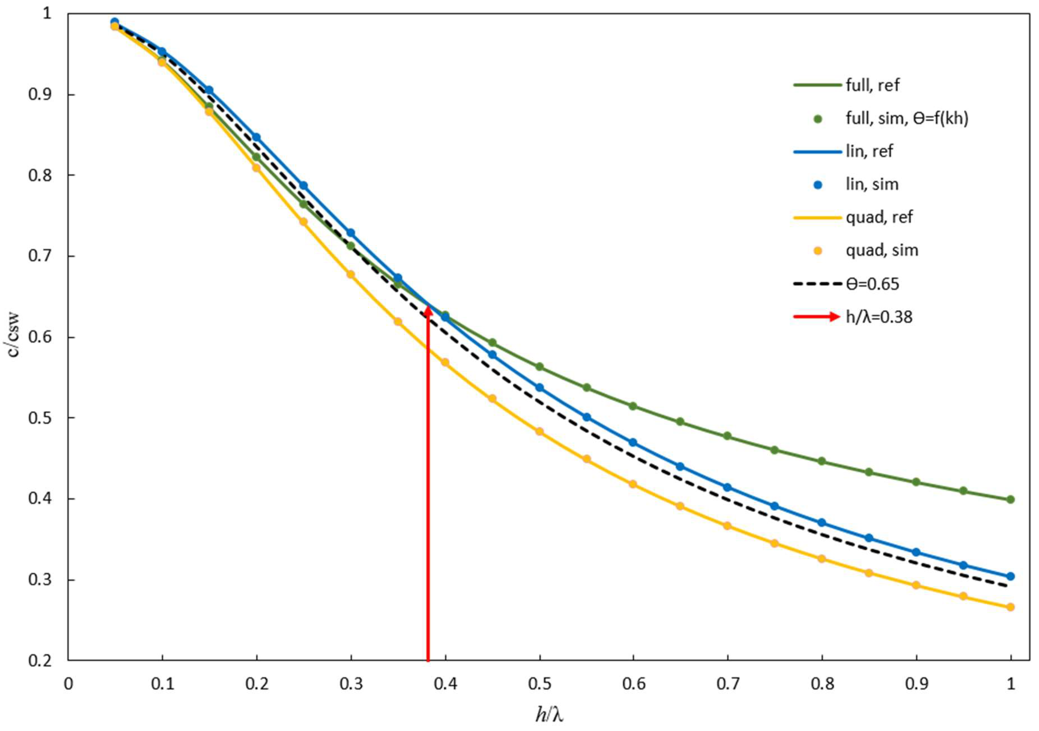
The numerical model was applied on a computational domain length equal to one wavelength. The periodic boundary conditions of Eq. [36] were imposed. The water depth, $h$, was varied while the wavelength $\lambda = {\displaystyle \frac{2\pi }{k}}=20$ m and the maximal amplitude a = 0.01 m were held constant to obtain ratios for ${\displaystyle \frac{h}{\lambda }}$ between 0.05 and 1.0, and ratios for ${\displaystyle \frac{a}{h}}$ between 0.01 and 0.005. The computational domain was discretized with a quadrilateral element mesh of sides ∆x = ∆y = 5 cm. Simulation time was one wave period.

Figure 1 displays the normalized phase velocities resulting from applying the non-hydrostatic Eqs. [23]-[26] with either the linear ($\mathrm{Ө}$= 1), the quadratic ($\mathrm{Ө}$= 0) or the weighted average linear/quadratic ($\mathrm{Ө}=\mathrm{f}\left(kh\right)$) vertical pressure. Additionally, they are compared to their analytical reference phase velocities obtained from Eqs. [29] and [30], and the full reference phase velocity obtained from Eq. [31]. All numerical dispersion relations accurately match the corresponding analytical ones, highlighting the case of the full linearized equations and the non-hydrostatic Eqs. [23]-[26] where the values of $\mathrm{Ө}=\mathrm{f}\left(kh\right)$ are calculated by Eq. $[32]$.

In the application of Eqs. [23]-[26] to the cases of variable bathymetry, only values of $\mathrm{Ө}$calculated by Eq. $[32]$ in the interval 0 ≤ ${\displaystyle \frac{h}{\lambda }}$ ≤ 0.38 were used (Figure 1). This is because averaging must occur within the limits of the two models (quadratic and linear; 0 ≤ $\mathrm{Ө}$ ≤ 1) whose applicability is verified. The value of $\mathrm{Ө}$ that minimizes the sum of the absolute deviations from the full reference phase velocity in the range 0 ≤ ${\displaystyle \frac{h}{\lambda }}$ ≤ 0.38 is $\mathrm{Ө}$= 0.65, as shown in Figure 1.

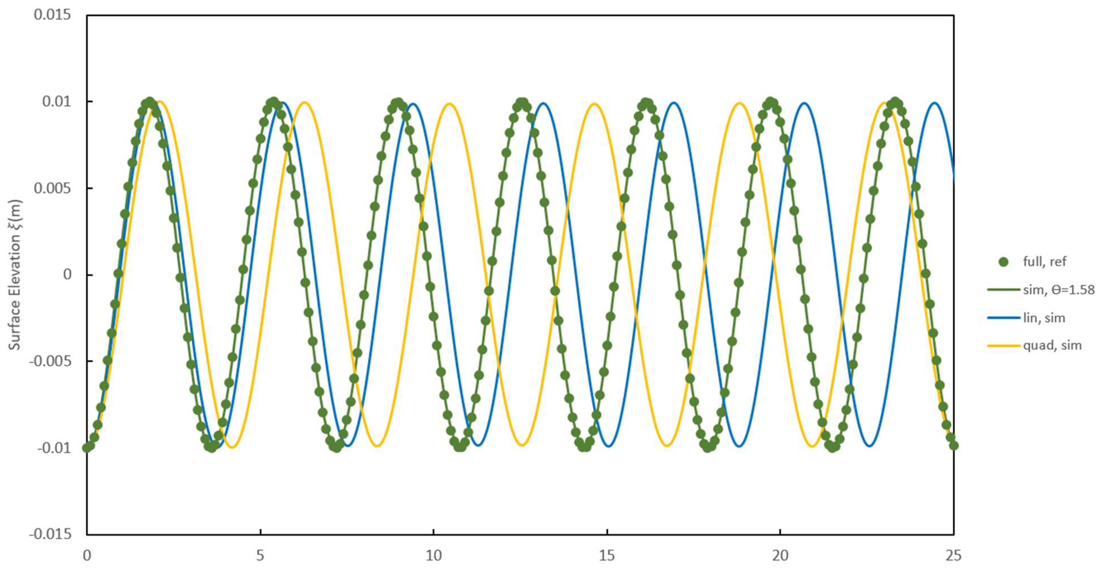
For a longer simulation time of 25 seconds, Figure 2 shows a time series of the surface elevation for the linear, the quadratic, and the weighted average linear/quadratic ($\mathrm{Ө}=1.58$) vertical pressures profiles evaluated at $x$ = 5 m, whereas a ratio of depth to wavelength of 0.5 is employed. As shown in Figure 2, the linear and quadratic pressure profiles lag behind the analytical solution, in particular the quadratic profile, while the weighted average linear/quadratic pressure profile can reproduce precisely the evolution of the water height.

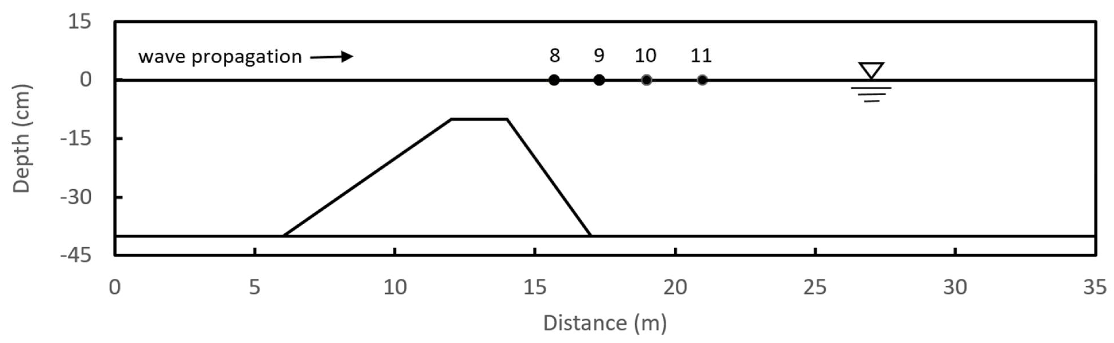
5. Beji and Battjes’ Experiment of Wave Propagation on a Submerged Bar

Beji and Battjes (1993) conducted physical experiments on the propagation of regular waves on a trapezoidal bar submerged in a channel 37.7 m long, 0.8 m wide, and 0.75 m deep.

Figure 3 shows the numerical setup of the experiment. The depth of still water is 0.4 m. A 0.3 m high trapezoidal bar, with a front slope of 1:20 and a back slope of 1:10, is located between 6 and 17 m in the channel. Incident sinusoidal waves with an amplitude of 1.0 cm and a period of 2.02 sec, corresponding to the parameter $kh$ = 0.67 $\left({\displaystyle \frac{h}{\lambda }}=0.11\right)$, are generated on the left side based on the linear wave theory. The boundary of the experiment on the right side is modeled as an open flow area where a Sommerfeld radiation condition is imposed. The non-hydrostatic pressure $q_b$is assumed to be zero on the left and right sides. The figure’s 35 m long computational domain is discretized with a quadrilateral element mesh of sides Δx = Δy = 1.25 cm. At the beginning of the simulation, the velocity and water surface elevation are zero at all nodes, and a short time interval Δt = 0.002 sec is used to develop the wave smoothly.

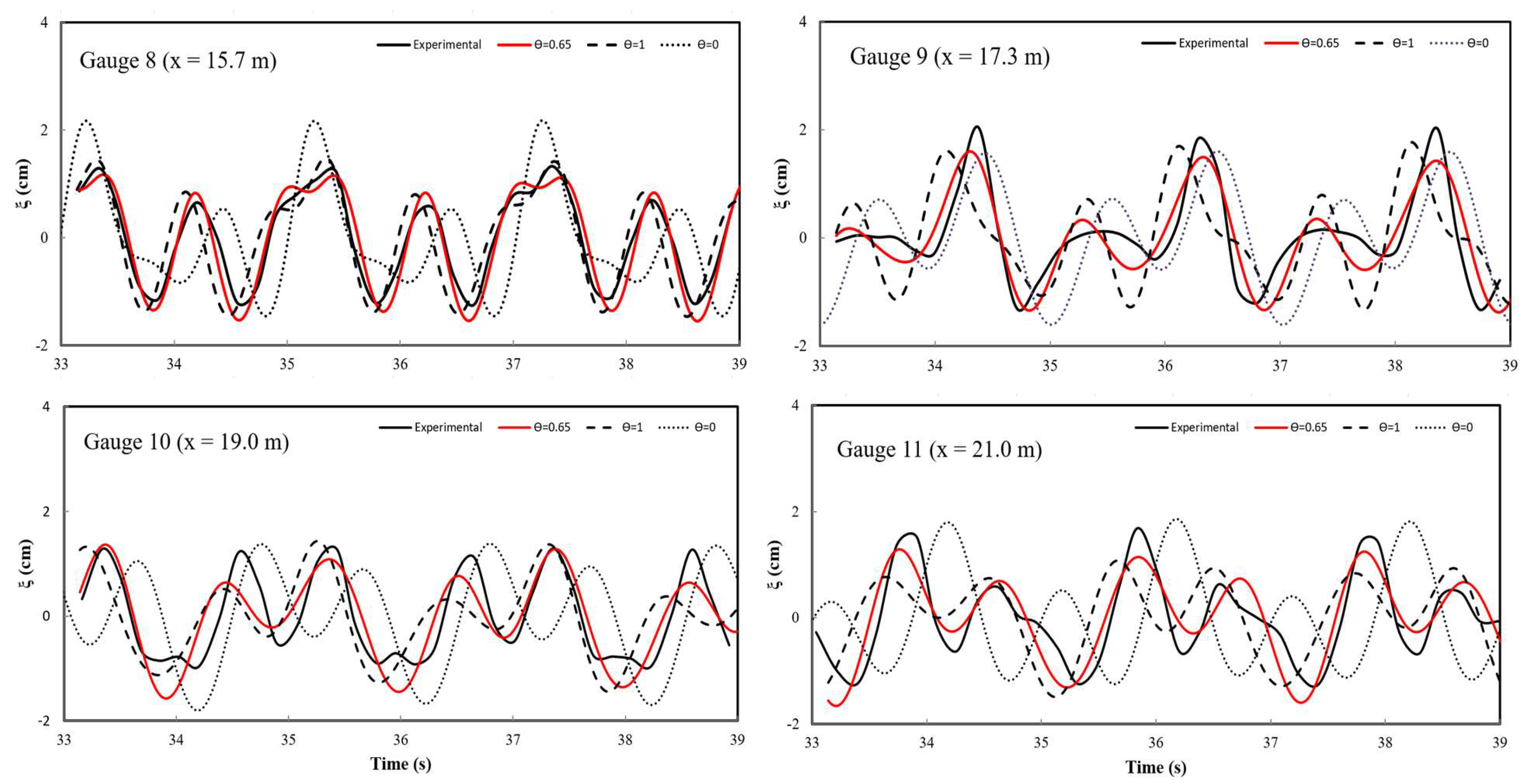
Figure 4 compares simulated and measured free surface elevations at measurement points 8, 9, 10, and 11 in Figure 3. The weighted average linear/quadratic profile using $\mathrm{Ө}$ = 0.65 improves the comparisons between measured and simulated wave elevations in all four measurement points.

= 0.65 (red line), linear profile: $\mathrm{Ө}$ = 1 (dashed line), quadratic profile: $\mathrm{Ө}$ = 0 (dotted line).

6. Whalin’s Wave Diffraction Experiment on a Semicircular Shoal and Comparison with Experimental Data

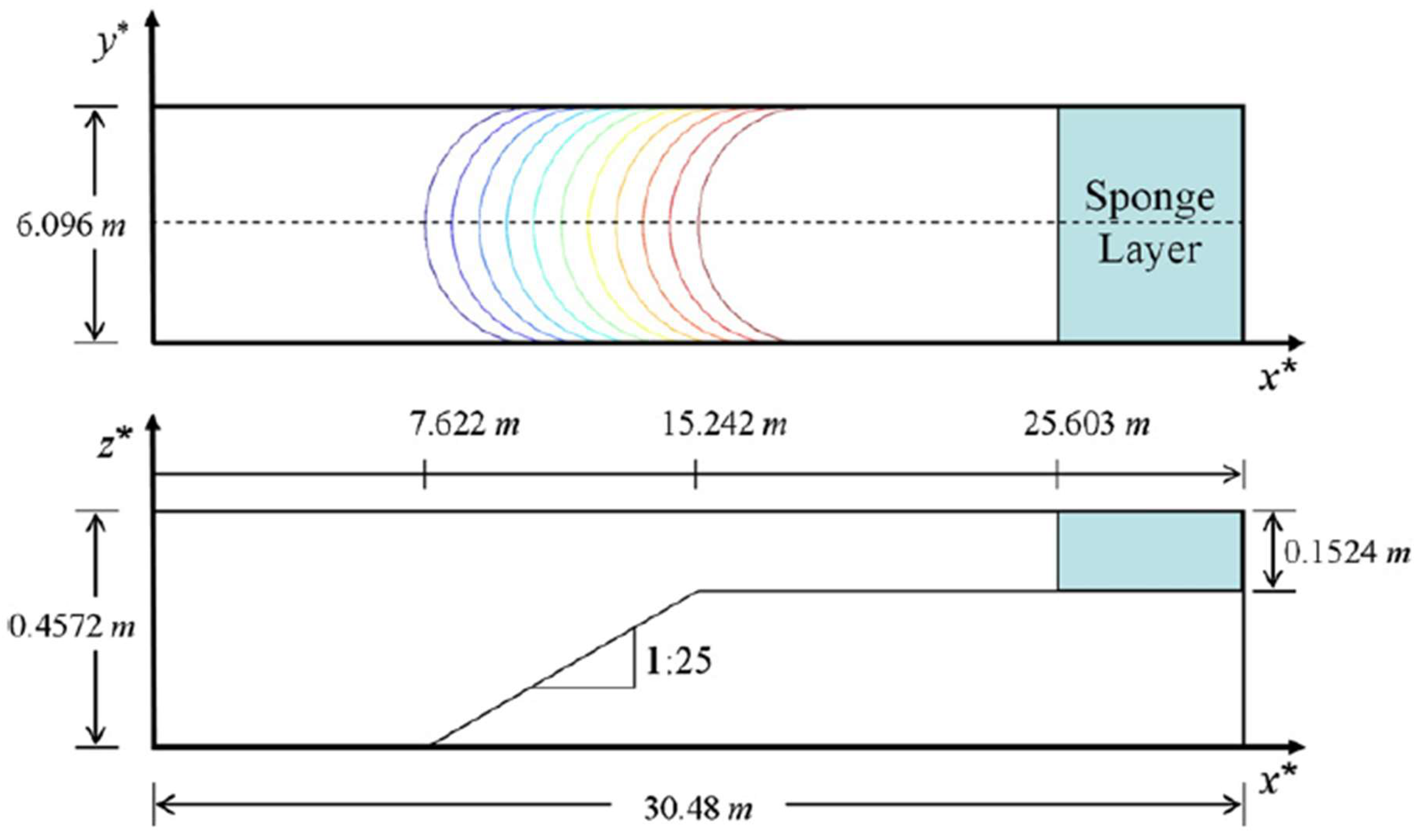
Whalin (1971) conducted laboratory experiments on wave refraction over a semicircular sloping bathymetry. The experiments used a wave tank 25.603 m long and 6.096 m wide (Figure 5). At the beginning of the tank, the water depth was 0.4572 m, while in the middle portion, 7.622 m ≤ $x^{*}$≤ 15.242 m, eleven semicircular steps were regularly spaced, arriving at the shallowest portion with a water depth of 0.1524 m.

The bathymetry was symmetrical to the tank centerline at $y^{*}=3.048 \mathrm{m}$ and was described by:

$$h\left(x^{\mathrm{*}},y^{\mathrm{*}}\right)=\left\{\begin{array}{c}0.4572 0\le x^{\mathrm{*}}\le 10.67-G \\ {\displaystyle \frac{\left(0.4572+10.67-G\right)}{25}} 10.67-G\le x^{\mathrm{*}} \le 18.29-G [37]\\ 0.1542 x^{\mathrm{*}} \le 18.29-G \end{array}\right.$$

$$G\left(y^{\mathrm{*}}\right)=\sqrt{y^{\mathrm{*}}\left(6.096-y^{\mathrm{*}}\right)}[38]$$

where $x^{*}$ and $y^{*}$are length variables in meters.

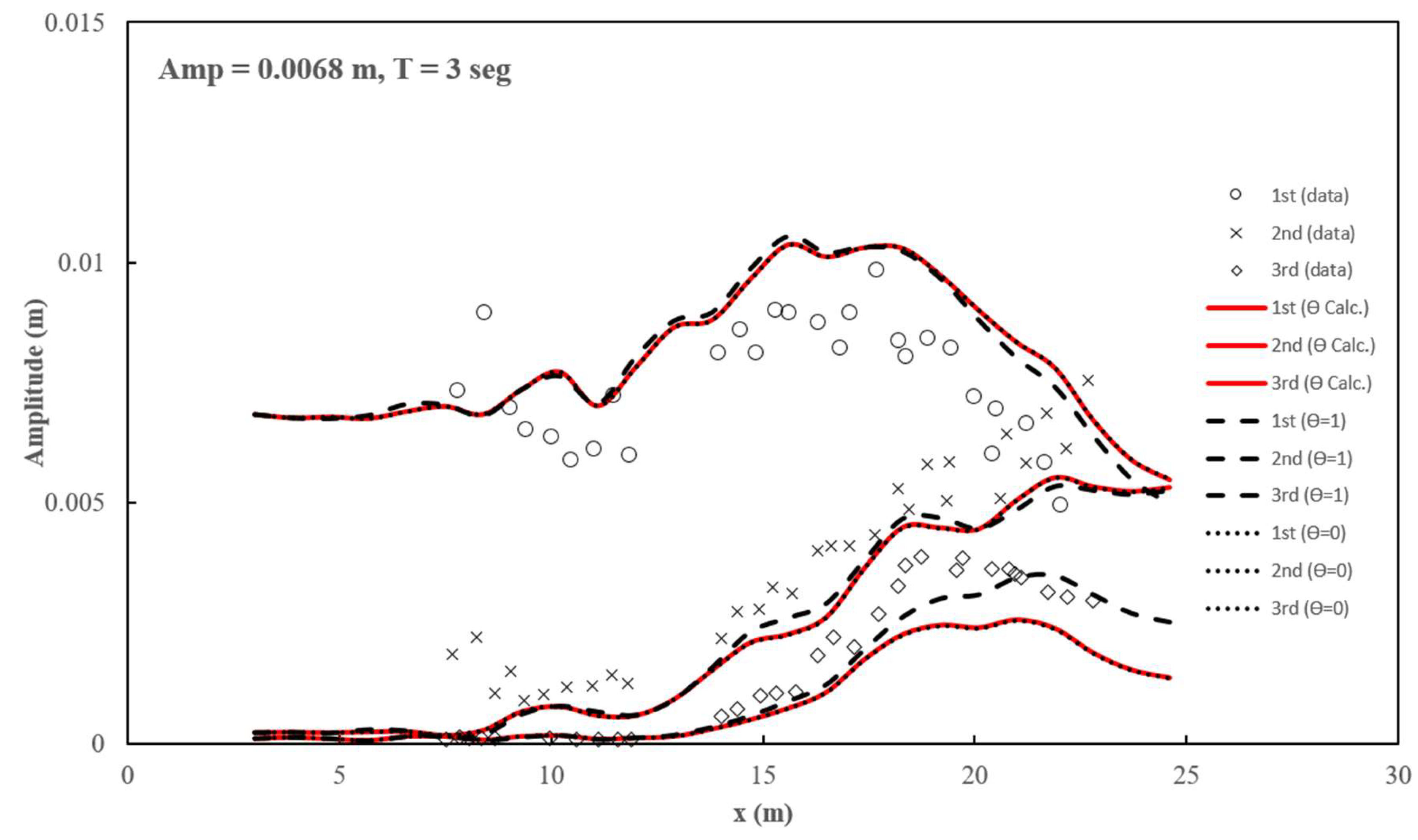
Three series of experiments were carried out generating waves with different periods T and wave amplitudes a:

Case I: T = 3.0 sec, a = 0.0068m, $\left({\displaystyle \frac{h}{\lambda }}=0.07\right)$;

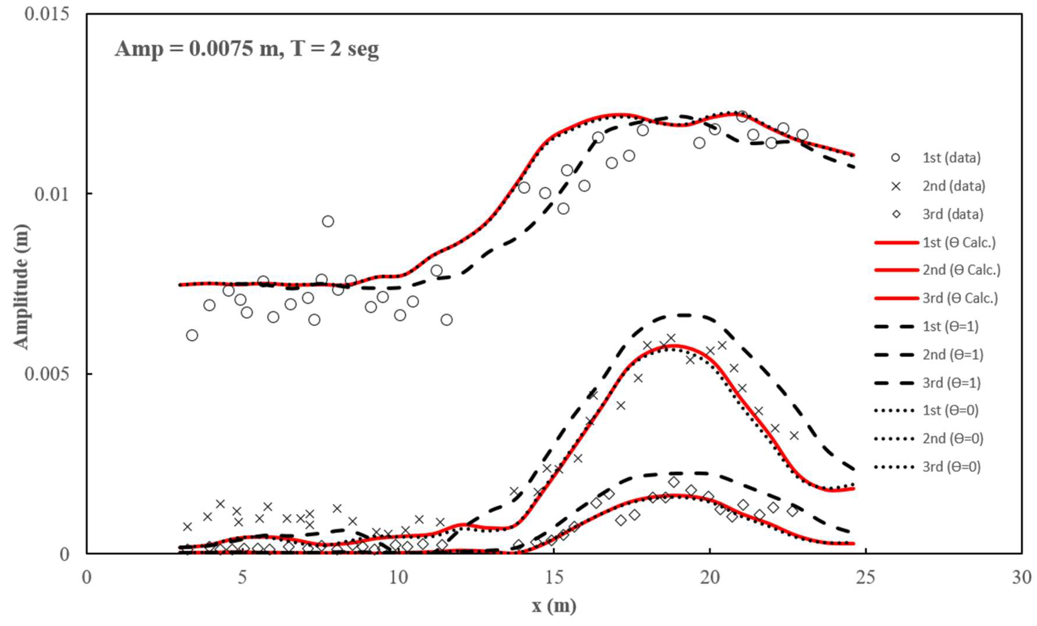
Case II: T = 2.0 sec, a = 0.0075m, $\left({\displaystyle \frac{h}{\lambda }}=0.12\right)$;

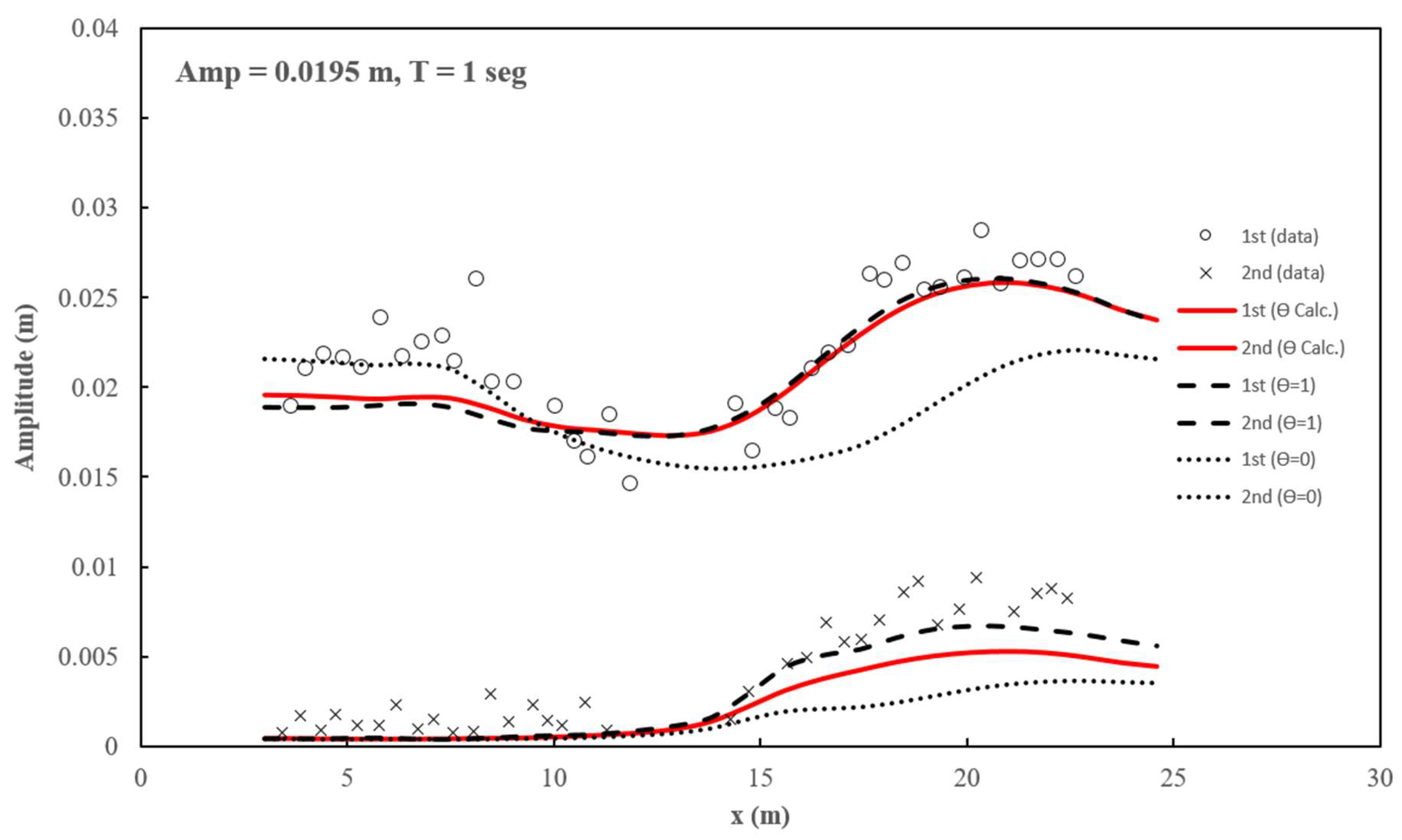
Case III: T = 1.0 sec, a = 0.0195m, $\left({\displaystyle \frac{h}{\lambda }}=0.31\right)$.

An incoming periodic wave train was generated in a 5 m generation zone. Sponge layers were applied upstream and downstream to absorb the outward and reflected waves, and solid wall boundary conditions were applied at the lateral boundaries. A mesh with Δx = 5 cm and Δy = 10 cm was used for the case I and II tests. For the test of case III, Δx = 2.5 cm and Δy = 10 cm were used, as this was the most intense case. Wave propagation was simulated for 100 sec, and numerical data were obtained for the last 25 sec. After measuring water surface elevation along the centerline of the shoal, a harmonic analysis was made to obtain the amplitude of the frequency components. The surface elevation time series along the midline was analyzed to obtain the amplitudes of the first, second, and third harmonics considering their spatial evolution. The numerical results were compared with the experimental data in Figure 6, Figure 7, and Figure 8. These simulations also tested the utilization of parameter $\mathrm{Ө}$ calculated using Eq. [32] with the wavelength, λ, calculated with Eq. [34].

For case I, some differences were observed between numerical results and experimental data (Figure 6). Similar results were observed in preceding studies (Bingham et al., 2009; Tonelli and Petti, 2009; Kazolea et al., 2012) and are usually attributed to reflected waves.

In case II, considerable improvements are observed in the comparisons between observed and simulated harmonics using the parameter $\mathrm{Ө}$ calculated through equations [32] and [34] (red lines in Figure 7).

For case III (Figure 8), the relatively high ${\displaystyle \frac{h }{\lambda }}$= 0.31 ratio of the incident wave leads to better model performance using $\mathrm{Ө}$ = 1 (linear non-hydrostatic pressure profile), particularly at the end of the ramp (x > 15 m). This could be because wave shoaling decreases wavelength λ, resulting in a further increase in ${\displaystyle \frac{h}{\lambda }}$, in addition to the wave’s nonlinearity in this zone.

7. Wave Transformation over an Elliptic Shoal

The transformation of waves over a submerged elliptical bank is a typical example for evaluating numerical models that simulate wave refraction, diffraction, and focusing. Non-hydrostatic models have been applied to simulate the wave transformation on an elliptical shoal. The non-hydrostatic 3D models can simulate wave propagation using a multigrid solver (Li and Fleming, 2021) or a small number of vertical layers (Stelling and Zijlema, 2003; Yuan and Wu, 2004; Zijlema and Stelling, 2005).

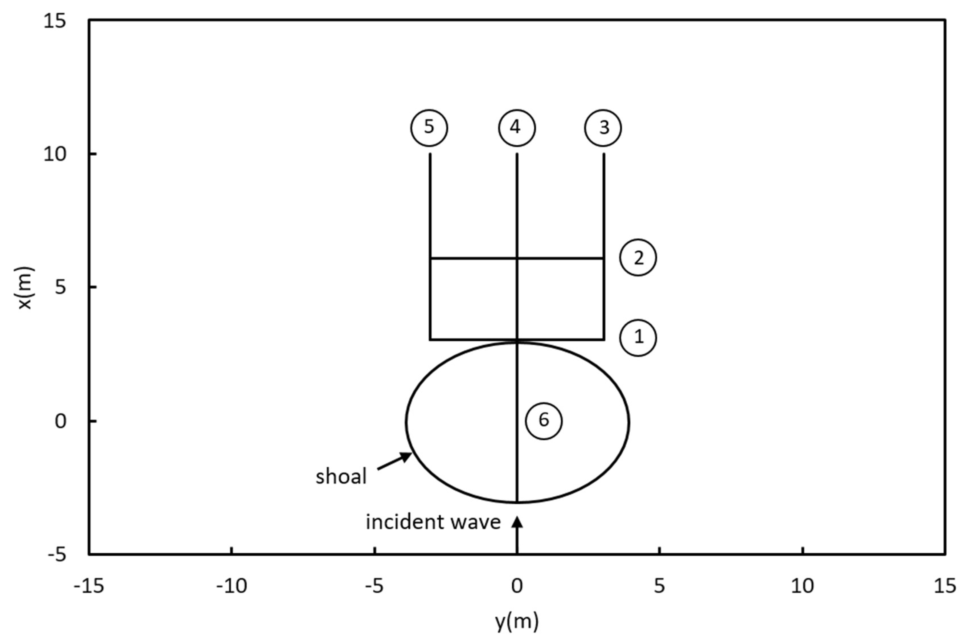
Figure 9 shows the experimental setup of Vincent and Briggs (1989), consisting of an elliptical shoal. The mathematical expression of the shoal boundary can be defined as:

$${\left({\displaystyle \frac{x}{3.05}}\right)}^2+{\left({\displaystyle \frac{y}{3.96}}\right)}^2=1[39]$$

And the depth over the elliptical shoal, $h_e$, is given by:

$$h_e=0.9144-0.762\sqrt{1-{\left({\displaystyle \frac{x}{3.81}}\right)}^2-{\left({\displaystyle \frac{y}{4.95}}\right)}^2}[40]$$

The constant water depth outside the elliptical shoal zone is ${ h}_0$ = 0.457 m. 17 incident wave conditions were investigated, from non-breaking monochromatic waves to breaking directional spectra. Surface displacements were measured at the six cross-sections shown in Figure 9. A non-breaking monochromatic incident condition was used in the model simulations. At the incoming boundary, an incident wave with height $H_0$ = 2.54 cm and period T = 1.3 sec was applied, corresponding to the ratio ${\displaystyle \frac{h}{\lambda }}=$

0.2. At the outgoing boundary, a 5 m absorption zone dissipated outgoing waves. The free-slip and impermeability boundary conditions were assigned to the sidewalls. The computational domain was discretized by a mesh with Δx = 5 cm and Δy = 10 cm.

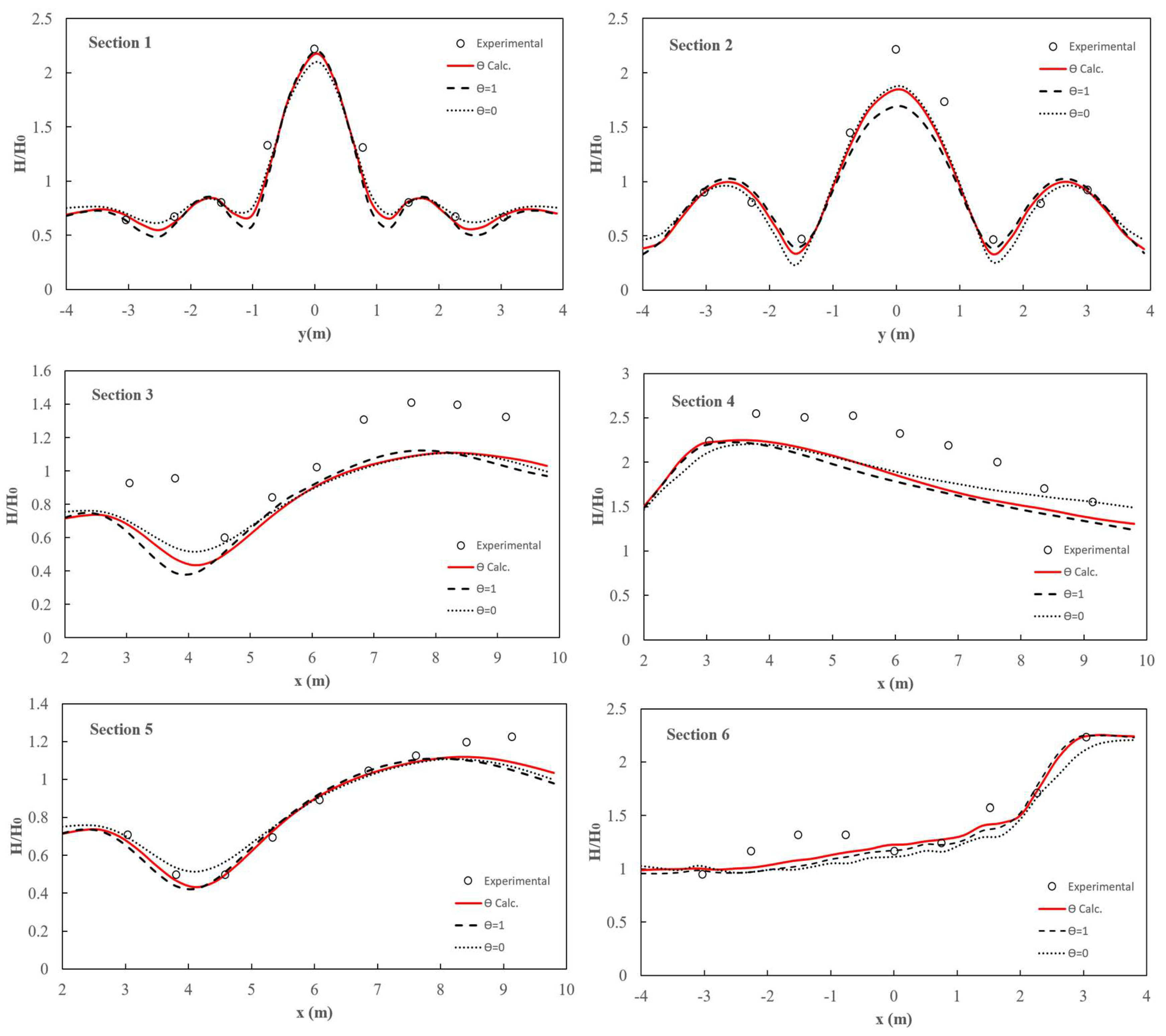
Figure 10 shows the model results compared to the experimental data regarding the normalized wave heights $\left(H/H_0\right)$ at the six cross sections in Figure 9. The calculated wave height was obtained by averaging the wave heights over five steady wave periods.

The model accurately predicted the wave concentration behind the bank in section 1, mainly using the parameter $\mathrm{Ө}$ calculated through equations [32] and [34]. In section 2, the model does not reach the experimental wave height due to the limitations inherent to vertically averaged models and the dissipative characteristic of the first-order explicit temporal approximation used in non-hydrostatic models (Wei 2014, Zijlema et al., 2011). In sections 4 and 6, along the direction of wave propagation, the wave steepens, and the interaction of the refracting wavefronts creates a maximum wave height around x = 4 m. After this point, the wave amplitude decreases due to the lateral propagation of the wave energy in sections 3 and 5. Figure 10 shows that utilizing a calculated $\mathrm{Ө}$ parameter generally improved comparisons between measured and simulated wave heights.

8. Conclusions

A new two-dimensional depth-integrated non-hydrostatic model for wave propagation simulation using a weighted average linear/quadratic non-hydrostatic pressure profile has been developed. The model is established by altering the non-hydrostatic discontinuous/continuous Galerkin finite element model with a linear vertical non-hydrostatic pressure profile described in Calvo et al. (2021).

A series of numerical tests have been carried out to verify and validate the developed model. The first case, with an analytical solution, was the simulation of a linear standing wave in one spatial dimension with constant bathymetry, which validated the model’s dispersive proprieties. The following three sets of laboratory experiments, which present several nearshore wave propagation phenomena (wave propagation on a submerged bar, wave diffraction on a semicircular shoal, and wave transformation over an elliptic shoal), have been used to validate the model’s capability for nearshore wave simulation.

Using a weighted average linear/quadratic non-hydrostatic pressure profile improved the performance of previous models with linear or quadratic non-hydrostatic pressure profiles. The results show that utilizing a weighted average linear/quadratic non-hydrostatic pressure profile, using a calculated or optimized $\mathrm{Ө}$ weight parameter, enhanced comparisons between measured and simulated wave heights in depth-integrated non-hydrostatic models.

Future work will continue with further analysis of the model in cases of variable bathymetry and comparisons with traditional Boussinesq-type models.

References

- Aïssiouene, N. (2016). Numerical analysis and discrete approximation of a dispersive shallow water model. PhD thesis. Pierre et Marie Curie, Paris VI.
- Bai, Y., Cheung, K.F. (2013). Dispersion and nonlinearity of multi-layer non-hydrostatic free-surface flow. J. Fluid Mech. 726, 226–26. [CrossRef]
- Beji, S.; Battjes, J. A. (1993) Experimental investigation of wave propagation over a bar. Coastal Eng. 19, 1, 151–162. [CrossRef]
- Bingham, H.B.; Madsen, P.A.; Fuhraman, D.R. Velocity potential formulations of highly accurate Boussinesq-type models. Coastal Engineering, 56, 467–478, 2009.
- Calvo, L., De Padova, D., Mossa, M., Rosman, P. (2021). Non-hydrostatic discontinuous/continuous Galerkin model for wave propagation, breaking and runup. Computation. 9, 47. [CrossRef]
- Casulli, V., Stelling, G.S. (1998). Numerical simulation of 3D quasi-hydrostatic, free-surface flows. J. Hydraul. Eng. 124, 678–686. [CrossRef]
- Cui, H., Pietrzak, J., Stelling, G. (2014). Optimal dispersion with minimized Poisson equations for non-hydrostatic free surface flows. Ocean Modelling 81, 1–12. [CrossRef]
- Fenton, J.D.; McKee W.D. On calculating the lengths of water waves. Coastal Engineering, 14, 499-513, 1990. [CrossRef]
- Jeschke, A., Vater, S., Behrens, J. (2017). A discontinuous Galerkin method for non-hydrostatic shallow water flows. In Proceedings of the Conference: Finite Volumes for Complex Applications VIII-Hyperbolic, Elliptic and Parabolic Problems, Lille, France, 12–16 June 2017.
- Jeschke, A. (2018). Second Order Convergent Discontinuos Galerkin Projection Method for Dispersive Shallow Water Flows. University of Hamburg, Phd Thesis, 2018.
- Kazolea, M.; Delis, A. I.; Nikolos, I. K.; Synolakis, C. E. An unstructured finite volume numerical scheme for extended 2D Boussinesq-type equations, Coastal Eng., 69, 42–66, 2012. [CrossRef]
- Stansby, P.K., Zhou, J.G. (1998). Shallow-water flow solver with non-hydrostatic pressure: 2D vertical plane problems. Int. J. Numer. Methods Fluids, 28, 541–563.
- Stelling, G.; Zijlema, M. An accurate and efficient finite difference algorithm for non-hydrostatic free surface flow with application to wave propagation. Int. J. Numer. Methods Fluids 2003. 43, 1–23, 2003. [CrossRef]
- Tonelli, M.; Petti, M. Hybrid finite volume -finite difference scheme for 2DH improved Boussinesq equations, Coastal Eng., 56, 609–620, 2009. [CrossRef]
- Vincent, C.; Briggs, M. (1989). Refraction-Diffraction of Irregular Waves over a Mound. [CrossRef]
- Journal of Waterway, Port, Coastal and Ocean Engineering, 115(2), 269-284.
- Wang, W., Martin, T., Kamath, A., Bihs, H. (2020). An improved depth-averaged non-hydrostatic shallow water model with quadratic pressure approximation. Int. J. Numer. Methods Fluids.
- Wang, W., Kamath, A., Martin, T., Pákozdi, C., Bihs, H. (2020). A comparison of different wave modelling techniques in an open-source hydrodynamic framework. J. Mar. Sci. Eng. [CrossRef]
- Wei, Z.; Jia, Y. (2014). Simulation of nearshore wave processes by a depth-integrated non-hydrostatic finite element model. Coast. Eng. 83, 93–107.
- Whalin, R.W. The limit of applicability of linear wave refraction theory in a convergence zone. Res. Rep. H-71-3, U.S. Army Corps of Engineers, Waterways Expt. Station, Vicksburg, MS. 1971.
- Young, C.; Wu, C.; Liu W.; Kuo J. A higher-order non-hydrostatic σ model for simulating non-linear refraction–diffraction of water waves. Coastal Engineering, 56 (9), 919-930, 2009.
- Yuan, H.L.; Wu, C.H. An implicit 3D fully non-hydrostatic model for free-surface flows, Int. J. Numer. Meth. Fluids 46, 709–733, 2004.
- Zijlema, M.; Stelling, G.S. Further experiences with computing non-hydrostatic free-surface flows involving water waves. Int. J. Numer. Methods Fluids. 48, 169–197, 2005. [CrossRef]
- Zijlema, M.; Stelling, G.S. Efficient computation of surf zone waves using the nonlinear shallow water equations with non-hydrostatic pressure. Coast. Eng. 55, 780–790, 2008. [CrossRef]
- Zijlema, M.; Stelling, G.S.; Smith, P. SWASH: An operational public domain code for simulating wave fiels and rapidly varied flows in coastal waters. Coast. Eng. 58, 992–1012, 2011.
Figure 1.
Periodic standing wave: Comparison of simulated non-hydrostatic phase velocities with analytic reference values.
Figure 2.
Periodic standing wave: Comparison of the simulated (green, blue, and yellow lines) and analytical (green dots) surface elevation with linear, quadratic, and weighted average linear/quadratic vertical profile for a propagation time of 25 seconds at location
Figure 3.
Numerical configuration for wave propagation over a submerged bar.
Figure 4.
Comparison of simulated elevations and free surface measurements for the case of wave propagation over a submerged bar. Experiment (black line), linear/quadratic profile: = 5 m with = 0.5.
Figure 5.
Bottom configuration for wave propagation over a semicircular shoal used in the experiments of Whalin (1971) (Source: Young et al., 2009).
Figure 6.
Periodic waves over a semicircular shoal (Case I): Comparison of simulated and experimental results for the wave amplitudes of harmonics 1, 2, and 3 along the centerline. Experiment (circles), linear/quadratic profile: calculated by Eq. [32] (red line), linear profile: = 1 (dashed line), quadratic profile: = 0 (dotted line).
Figure 7.
Periodic waves over a semicircular shoal (Case II): Comparison of simulated and experimental results for the wave amplitudes of harmonics 1, 2, and 3 along the centerline. Experiment (circles), linear/quadratic profile: calculated by Eq. [32] (red line), linear profile: = 1 (dashed line), quadratic profile: = 0 (dotted line).
Figure 8.
Periodic waves over a semicircular shoal (Case III): Comparison of simulated and experimental results for the wave amplitudes of harmonics 1, 2, and 3 along the centerline. Experiment (circles), linear/quadratic profile: calculated by Eq. [32] (red line), linear profile: = 1 (dashed line), quadratic profile: = 0 (dotted line).
Figure 9.
Schematic of the elliptical shoal and measurement sections.
Figure 10.
Comparison of simulated elevations and free surface measurements for the case of wave propagation over an elliptic shoal. Experiment (circles), linear/quadratic profile: calculated by Eq. [32] (red line), linear profile: = 1 (dashed line), quadratic profile: = 0 (dotted line).