Assessment of Analytical Methods for Estimating Settlements Induced by Side-by-Side Twin Tunnels

1. Introduction

In densely populated urban centers efficient and sustainable transportation networks are vital for economic development [1]. Factors such as the limited space at ground surface, traffic congestion and growing demands for sustainability and better environment have driven the construction and relocation of transportation networks into the subsoil [2]. Despite the complexity associated with the construction, these underground networks provide higher mobility and are more reliable and efficient than surface solutions making them a cost effectively asset for any city [3]. Solutions such as side-by-side twin tunnels, in opposition to the construction of a single larger tunnel, are often preferred for these infrastructures since traffic can flow separately in opposite directions, minimizing the congestion and number of collisions while maximizing the speed and safety of travelling. The excavation process itself is often simpler in this case, as the construction of smaller tunnels is quicker, requires less support and can be performed at shallower depths, reducing the costs without compromising the stability and safety of the excavations.

However, regardless of the construction method employed, the excavation of tunnels will inevitably induce movements in the surrounding soil, which, in shallower tunnels, extend to the ground surface and affect the structures located in the vicinity of the excavation [4]. Naturally, the magnitude and extent of those ground movements are influenced by several factors, such as the tunnel geometry, the soil and groundwater conditions and the excavation method employed [5]. In order to perform an adequate risk assessment of the structures during the preliminary design stage a quick yet reliable estimation of the magnitude and extent of the ground movements induced by the tunnels excavation is required [6, 7]. For a single tunnel excavation the typical settlement profile is well documented in the literature and, amid other proposals [8], can be reasonably approximated as an inverted Gaussian distribution curve, as suggested by Peck [9]. However, the case of side-by-side twin tunnels is more complex with several studies (see Table 1) showing that the excavation of the second tunnel (2T) induces higher settlements when compared with those caused by the construction of the first tunnel (1T). Moreover, it has been observed that the final settlement trough shows some asymmetry, with the maximum settlement occurring closer to the 1T, rather than being centered between the tunnels [10-12]. According with Mair and Taylor [7] this interaction effect occurs since the 2T is excavated in disturbed ground conditions and is fundamentally dependent of the distance between tunnels, usually referred as pillar width (P). However, recent advances in EPB (earth pressure-balanced shields) technology, have made it possible to adjust shield operational parameters, such as the face or grouting pressure, so that the settlements induced by the 2T excavation can be compensated and reduced significantly, as the results of Suwansawat and Einstein [13] have demonstrated.

The interaction between side-by-side twin tunnels has been widely documented in various case studies (see Table 1) but has also been investigated through numerical [14-24], centrifuge [4] and small-scale models [25-28]. An extensive compilation and review of those studies has already been presented and summarized by Vlachopoulos, et al. [29] and more recently by Islam and Iskander [5]. These studies assess aspects such as the lining forces interaction [30, 31], the overall tunnels stability [32, 33] and the stress redistribution along the pilar width [34, 35], but are primarily focused on evaluating the ground movements and volume loss induced by the excavation of the 2T and on assessing the distance between tunnels at which interaction effects can be considered negligible. Based on the results provided by those studies several analytical methods have been proposed to quantify the settlements and sub-surface vertical displacements caused by side-by-side twin tunnel excavation [4, 16, 22, 36-40]. Despite the differences among them, all proposals assume that the settlement profile induced by the excavation of the 1T is described by an inverted Gauss distribution curve and use those Gaussian fitting parameters, along with the distance between tunnels, to predict the additional volume loss induced by the 2T excavation. Although these analytical methods are of simple application and can provide valuable insights during the preliminary design stage, they were developed for specific cases, and their applicability to real case studies has yet to be fully validated. This paper discusses the applicability of those analytical methods by comparing their prediction against the monitoring data reported for a vast number of case studies published in the literature. The aim of this paper is to highlight the strengths and limitations of each of those analytical methods, enabling more informed decision-making when predicting settlements induced by twin tunnelling.

2. Materials and Methods

2.1. Analytical Methods for Predicting Ground Movements Induced by Twin Tunnelling

The first attempt to predict the settlements induced by side-by-side twin tunnelling was proposed by O'Reilly and New [36] and consisted on the superposition of two identical Gauss curves, each one aligned with the centerline of each tunnel, with the final settlement given as expressed by Equation 1:

$${\delta }_v\left(x\right)={\delta }_{v,max}·\left[e^{\left(-{\displaystyle \frac{x^2}{2·i^2}}\right)}+e^{\left(-{\displaystyle \frac{{(x-d)}^2}{2·i^2}}\right)}\right]$$

(1)

where $d$ represents the distance between the centrelines of the tunnels, $x$ is the horizontal distance measured from the centerline of 1T (note that 1T is assumed as being located on the left hand side), and ${\delta }_{v,max}$ and $i$ are the Gauss parameters, with ${\delta }_{v,max}$ corresponding to the maximum settlement estimated at the tunnel centerline and $i$ to the trough width parameter, which represents the distance from the centerline to the inflection point of the Gauss curve. In the absence of field data, the estimation of the Gauss parameters is usually performed using correlations established in the literature. The trough width parameter is usually correlated with the depth of the axis of the tunnel ($Z_0$) by Equation 2:

$$i=K·Z_0$$

(2)

where $K$ is the dimensionless trough width factor, whose value depends on the soil characteristics [7, 36]. According to Mair and Taylor [7], $K$ typically ranges between 0.4 to 0.6 in clays and 0.25 to 0.45 for granular materials, with the average values of these intervals often taken as representative. The value of ${\delta }_{v,max}$ is typically determined using Equation 3 and having as reference the estimated volume loss, $V_s$ (expressed as a percentage of tunnel face volume per unit length of tunnel).

$${\delta }_{v,max}=\sqrt{{\displaystyle \frac{\pi }{32}}}·{\displaystyle \frac{V_s·D^2}{i}}$$

(3)

where $D$ is the tunnel diameter. $V_s$ depends on the tunnel characteristics, soil conditions and excavation method, with reported values varying between 0.1 and 3.3% [5]. Naturally, with the recent advances in technology it is possible to reduce $V_s$ to almost zero if adequate shield operational parameters are employed when excavating with a EPB machine [41].

The equation proposed by O'Reilly and New [36] assumes that both tunnels induce the same $V_s$, implicitly disregarding any interaction between them. As a result, this proposal is only acceptable when the tunnels are reasonably spaced apart (pillar to diameter (P/D) ratio greater than 4) or when the tunnels are driven almost simultaneously [42]. While still used as reference, several studies have shown that O'Reilly and New [36] proposal is not adequate for estimating settlements induced by side-by-side twin tunnels, as interaction effects between the tunnels are not considered.

To assess the interaction between side-by-side tunnels, Addenbrooke and Potts [16] conducted a series of coupled consolidation 2D numerical analyses, where the distance between tunnels centerlines ($d$), was varied from 8 to 32m (P/D between 1.0 and 7.0). Based on the results obtained the authors proposed the design chart presented in Figure 1 to adjust the volume loss associated with the 2T ($V_{s,2T}$) having as reference the value obtained in greenfield conditions for the 1T excavated ($V_{s,1T}$). The correction factor reached a maximum of about 25% for the lowest P/D analyzed and then gradually decreased as the distance between tunnels increased, becoming negligible for P/D ratios greater than 7. Addenbrooke and Potts [16] also observed that the 2T settlement trough presented an eccentricity towards the 1T and proposed a correction (Figure 1) to determine the offset of the maximum settlement of the 2T Gauss curve ($e_{2T}$) as a function of the tunnels spacing ($d$).

Also based on a numerical study and supported by a series of 1g 1/50 small-scale models Chapman, et al. [22] and Hunt [39] proposed the introduction of a modification factor, $F$, on the 2T Gauss curve in order to include the interaction effects (Equation 4).

$${\delta }_{v,2T}(x)=F·{\delta }_{v,max}·e^{\left(-{\displaystyle \frac{{(x-d)}^2}{2·i^2}}\right)}$$

(4)

The modification factor is defined by Equation 5 and decreases linearly between a maximum value (1.6 to 1.8), directly above the centerline of the 1T, to 1.0 as the distance from the 1T centerline increases. In Equation 5, the parameter $A$ corresponds to a multiple of the trough width parameter in a half settlement trough and is commonly set as 2.5 or 3 (with 3.0 adopted in this paper) while $M$ is the maximum modification factor, varying between 0.6 to 1.5, with a value of 0.6 recommended by Hunt [39].

$$F=\left[1+\left(M·\left(1-{\displaystyle \frac{d+x}{A·i}}\right)\right)\right]$$

(5)

However, according with Hunt [39], the modification factor should only be applied in the “overlapping zone” of the two settlement troughs, where the soil is assumed to have been disturbed by the excavation of the 1T (Figure 2). This correction results in an asymmetric settlement trough, with the maximum settlement of the 2T presenting some eccentricity towards the 1T, as suggested by Addenbrooke and Potts [16].

Divall [43] investigated the interaction of side-by-side twin-tunnels through a series of centrifuge tests. Based on their findings, the authors proposed a method similar to that presented by Addenbrooke and Potts [16], where the volume loss of the 2T ($V_{s,2T}$) was determined having as reference the greenfield results (volume loss of the 1T) and the distance between tunnels ($d$). The additional volume loss (${∆V}_{s,2T}$) induced by the 2T excavation can be calculated using Equation 6, while the volume loss of the 2T can be obtained by adding the additional volume loss to the volume loss induced by the 1T, as expressed in Equation 7. Also in this case, when the distance between centerlines of the tunnels increases, the interaction effect reduces and becomes negligible for $d/D>5.0$.

$${∆V}_{s,2T}=0.441·{\left({\displaystyle \frac{d}{D}}\right)}^{-1.062}·V_{s,1T}$$

(6)

$$V_{s,2T}=V_{s,1T}+{∆V}_{s,2T}$$

(7)

Although the maximum settlement was aligned with the centerline of the 2T, Divall and Goodey [4] observed an asymmetry in the shape of the 2T settlement trough with the side towards the 1T being wider when the tunnels were closely spaced, likely due to the soil disturbance in that zone as noted by Mair and Taylor [7]. To account for this effect Divall [43] proposed a correction to the dimensionless trough width factor ($K$), suggesting that in the side towards the 1T (inside zone) a value of 0.7 should be adopted for distances between centerlines of the tunnels smaller than 3D. In contrast, for the outside zone, the value obtained for greenfield conditions should be applied, regardless of the distance between tunnels. However, it should be noted that applying the correction proposed by Divall [43] results in a 2T volume loss greater than that calculated using Equations 6 and 7 since the settlement trough becomes wider in the inside zone, leading to an apparent inconsistency in the method.

Having as reference the construction data of the excavation of the Otogar-Kirazli line of the Istanbul Metro, Ocak [37] proposed a new analytical method for predicting settlements induced by twin tunnelling. Similar to the modification factor proposed by Chapman, et al. [22] and Hunt [39], Ocak [37] introduced a disturbance factor ($k$) to adjust the settlement trough induced by the 2T excavation. The disturbance factor, defined in Equation 8, is a function of the ratio between the distance between the tunnel centerlines and the tunnel diameter ($d/D$).

$$k=1+{\displaystyle \frac{D}{d}}$$

(8)

According with Ocak [37] both the trough width parameter and the maximum settlement associated with the 2T excavation should be multiplied by the disturbance factor, as expressed in Equations 9 and 10. In this method, similar to previous methods, the final settlement trough can be obtained by adding the adjusted 2T curve with the settlement curve predicted for greenfield conditions (1T).

$$i_{2T}=k·i$$

(9)

$${\delta }_{v,2T}(x)=k·{\delta }_{v,max}·e^{\left(-{\displaystyle \frac{{(x-d)}^2}{2·i_{2T}^2}}\right)}$$

(10)

Having as reference the field data of a twin tunnel excavation in Wuhan, Zhou, et al. [38] proposed a method very similar to that proposed by Chapman, et al. [22] and Hunt [39], with the main difference being that instead of a linear decrease of the modification factor, Zhou, et al. [38] adopted the exponential function expressed in Equation 11.

$$F=M·\left(e^{-{\displaystyle \frac{x^2}{2·i^2}}}-1\right)·{\left(1-e^{-{\displaystyle \frac{{(2·A·i)}^2}{8}}}\right)}^{-1}+1+M$$

(11)

In this expression the parameters $A$ and $M$ are analogous to those defined by Chapman, et al. [22] and Zhou, et al. [38] recommends the adoption of similar values. Also in this method the modification factor should only be applied in the “overlapping” zone, as defined in Figure 2. The settlements induced by the 2T can then be calculated using Equation 4, with the final settlements being obtained as in the previous methods, i.e., by summing the adjusted 2T curve with the settlement curve predicted for greenfield conditions (1T).

More recently, Dong, et al. [40] proposed a method where the settlements induced by the 2T were calculated by adding to the Gauss curve obtained in greenfield conditions an additional curve that accounts for the soil disturbance caused by the 1T construction. The authors proposed that this additional curve is located in the “overlapping” zone, centered above the midpoint between tunnels, and also follows a Gaussian shape. However, in this approach the “overlapping” zone is established considering both the soil layering and the plastic zone that develops around the tunnel during excavation. This implies that applying the method requires prior knowledge of not just the soil stratification but also the initial stress state and the strength parameters of all layers, making it cumbersome and impractical for early design assessments. Moreover, for the determination of the fitting parameters of the additional Gaussian curve, Dong, et al. [40] assumed a linear relationship between the additional volume loss and the volume loss induced by the 1T. This assumption is inadequate, as it neglects the influence of tunnel spacing. It implies that tunnels placed very close together or far apart would induce the same additional volume loss, which contradicts the findings from various case studies. For these reasons it was decided not to consider this method in this study.

To compare the settlements predicted by the different analytical methods a parametric study was conducted. For this purpose, twin tunnels with diameters ($D$) of 5m, with their axis located at a depth ($Z_0$) of 20m and spaced at distances ($d$) of 10, 20 and 30m (corresponding to P/D ratios of 1.0, 3.0 and 5.0, respectively) were considered. It was assumed that the Gaussian curve in greenfield conditions (1T) had an $i$ of 10m and a ${\delta }_{v,max-1T}$ of 10mm (equivalent to $V_s=1.28\%$). The settlements normalized by the maximum settlement (${\delta }_v/{\delta }_{v,max-1T}$) are plotted against the distance from the center line of the 1T normalized by tunnel diameter ($x/D$) in Figure 3 for the three P/D ratios considered. The upper plots correspond to the predictions of the settlement induced by the 2T, while the lower plots represent the final settlements obtained after combining the settlements induced by both tunnels. The greenfield settlement (1T) is also superimposed in the plots for reference.

The results show that all methods predict that the settlement induced by the 2T increases as the P/D ratio decreases, except for the method proposed by O'Reilly and New [36], which assumes no interaction between tunnels. Consequently, in this method the predicted settlements are in all cases equal to the greenfield ones. For a P/D=1.0, Ocak [37] method estimates an increase in the maximum settlement of about 50% compared to the reference value, whereas the other methods predict smaller increases ranging between 20 and 40%. As the P/D ratio increases, the predictions from all methods tend to become similar, with minimal interaction effects predicted for the P/D=5.0 ratio, except for the methods of Addenbrooke and Potts [16] and Ocak [37]. Notably Ocak’s [37] method also estimates wider settlement curves, leading to significantly higher volume loss estimates. As for the eccentricity of the maximum settlement towards the 1T, the method proposed by Addenbrooke and Potts [16] clearly predicts the highest values. In contrast, the other methods generally predict minimal eccentricities, apart from Ocak [37] and Divall [43], which do not consider any eccentricities. Naturally, as the P/D ratio increases the predicted eccentricities decrease, and by a ratio of 5.0 , they become negligible in most methods with the exception of the eccentricity predicted by Addenbrooke and Potts [16] method.

The final settlements displayed in the lower plots of Figure 3 are a consequence of the predictions made for the 2T. As a result of the large eccentricities predicted Addenbrooke and Potts [16] method, it estimates very large settlement troughs for the higher P/D ratios considered (3.0 and 5.0), with settlements being particularly higher across the entire pillar width between tunnels. For P/D=1.0, the Ocak [37] method predicts the largest settlement trough, both in terms of maximum displacement and width. All other methods result in similar final settlement troughs, with the interaction effect between tunnels reducing as P/D ratio increases. These results highlight the importance of the spacing between the tunnels in the prediction of the settlements induced by side-by-side twin tunnels.

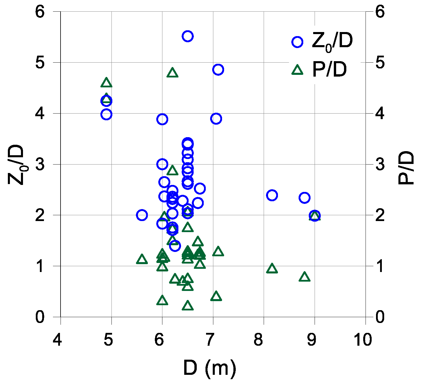
2.2. Case Studies and Physical Model Tests

The analytical methods proposed in the literature were derived based on limited data, which was mainly obtained through numerical modelling and physical modelling or by analyzing the monitoring data of a small number of case studies. As a result, the reliability of the proposals is confined to specific scenarios and their broader applicability has not yet been fully validated. However, with the increasing construction of underground transportation networks and the extensive dissemination tools available, there is now published in the literature a vast number of cases studies which reported quality monitoring data of settlements caused by side-by-side twin tunnelling excavations. A list of the collected case studies is presented in Table 1 and includes data from 19 projects, which totalize 46 sections where settlements were measured. Only cases where the tunnels and the monitoring alignments were perpendicular were considered, to avoid any effects related to the skew angle of the excavation, which are known to distort the typical Gaussian shape of the transverse settlement trough, making it asymmetrical [44]. Following the advances made in technology it is not surprising that almost all tunnels were excavated using EPB shields with only two projects identified as using sequential excavation. The ground conditions observed at the tunnel face varied significantly, ranging from medium stiff to stiff clays, silty soils, granular materials and soft rocks. The geometrical characteristics of the tunnels analyzed in the case studies are presented in Figure 4. The tunnel diameters ranged from 4.9 to 9.0m, with the vast majority falling between 6.0 and 6.5m. The depth to diameter ratio ($Z_0/D$) varied from 1.3 to 5.5, while the pillar width to diameter ratio (P/D) varies between 0.2 and 4.8, with most of the tunnels spaced 0.5 to 1.5 times their diameter apart. Overall, the geometrical space covered by the analyzed case studies is extensive, encompassing a wide range of P/D ratios.

Physical models of side-by-side twin tunnel excavations have also been reported in the literature. A total of four studies were identified, with their details summarized in Table 2. Of these, three studies involve small-scale models and one centrifuge testing, totalizing 11 tests with available data. The geometrical space covered by these tests spans from $Z_0/D$ values of 1.0 to 4.3, with P/D varying between 0.5 and 3.5. These tests have the advantage of being performed in a controlled environment, without the challenges associated with variable geological conditions and excavation operation factors. However, they present some limitations, such as the reduced stress state in the case of the small-scale models and the complexity of operating the centrifuge apparatus, in addition to the challenges associated with simulating the tunnels excavation mechanism, which differs in all studies.

3. Results and Discussion

3.1. Adjustment of the Gaussian Curves to the Settlement Data

The initial step in predicting twin-tunnel settlement using any analytical method involves adjusting a Gaussian curve that fits the settlements obtained in greenfield conditions, i.e., after the 1T excavation. In this study there was no need to estimate the Gaussian parameters using empirical expressions since the results from the case studies and physical models presented in Table 1 and 2 were available. In total, the settlements of the 57 listed sections were analyzed, and the parameters of the Gaussian curves (${\delta }_{v,max-1T}$ and $i_{1T}$) fitted by applying the least square method. The obtained parameters and corresponding fitting metrics are presented in Table A1 in Appendix A. In addition to the standard coefficient of determination (R²), calculated using Equation A1, the root mean squared error (RMSE) was also computed using Equation A2, as this metric provides a more interpretable and practical assessment of the fit. To evaluate if the settlements induced by the 2T excavation also followed a Gaussian shape, as suggested by some of the analytical methods [13, 38, 57], the data from this excavation (obtained by subtracting the settlements of the 1T to the final ones measured) was also fitted using a similar approach. Figure 5(a) presents the R² obtained for both 1T and 2T excavations. It can be observed that the quality of the fit of the 1T data is significantly higher, with R² values exceeding 0.9 for almost all analyzed sections. In contrast, the fit of the 2T data is lower, with many sections presenting a R² below 0.9. In order to improve the fit of the 2T data, an additional parameter was introduced in the calibration of the Gaussian curve, so that the maximum displacement could exhibit some eccentricity ($e_{2T}$) toward the 1T (considered positive), as suggested by Addenbrooke and Potts [16] and Hunt [39]. It should be noted that in some sections (see note 2 in Table A1) the best fit was obtained with an eccentricity directed toward the lateral side (negative eccentricity). In these cases, where atypical movements were observed, a null eccentricity was considered in the analyses, even if it did not provide the optimal fit. The obtained results are presented in Table A1 (Appendix A) with the corresponding R² values displayed in Figure 5(b). The results show a significant improvement in the fit, with the vast majority of sections reaching R² values above 0.9. A similar conclusion can be drawn from Figure 5(c), where the RMSE of both excavations is depicted. With the introduction of a free eccentricity the quality of the fit improved considerably, with most sections presenting RMSE values below 0.15. The sections with poorer fits are indicated in the figure (D1, E1, G1, G5, J, N2, P, Q and R1) and are all associated with atypical and/or asymmetrical movements observed on one of the lateral sides of the tunnels. Overall, the results confirm that both the 1T and 2T excavation appears to be adequately described by a Gaussian curve, which in the case of the 2T is eccentric.

The fitted Gaussian parameters for both the 1T and 2T are compared in Figure 6, with the data grouped by soil type for the analyzed cases studies and into a group comprising all results from the physical models to facilitate the interpretation. According to the analytical methods, it should be expected that both the maximum settlement (Figure6(a)) and the trough width parameter (Figure6(b)) would be larger for the 2T excavation, leading to higher volume losses (Figure6(c)). However, this is not the case in several sections, where the maximum settlement and, particularly, the trough width parameter are higher for the 1T excavation. As a result, in several sections (see note 15 in Table A1), the excavation of the 2T induced smaller volume losses than those observed in the 1T excavation. A detailed analysis of the studies where this condition occurred revealed two key factors that justify the results: i) atypical movements recorded on one side of the tunnel; ii) adjustments to shield operational parameters in the 2T excavation, such as face and grout pressure and penetration rate, which lead to smaller settlements (inclusively heave) and, consequently, smaller volume losses. This was the case observed in the Bangkok MRTA (case G) where Suwansawat and Einstein [13] highlighted the importance of controlling and adjusting the shield operational parameters in mitigating ground settlements. It is worth noting that no specific trend was observed regarding the type of soil with anomalies identified in nearly all groups considered.

For comparison with the empirical estimation of the Gauss parameters associated in the 1T excavation, the trough width factor ($K$) and the volume loss ($V_{s-1T}$) are plotted in Figure 7 against the normalized tunnel axis depth. The trough width factor value (Figure 7(a)) ranges from 0.2 to 0.9, with the majority of the cases concentrated between 0.3 and 0.6, as indicated by Mair and Taylor [7]. Also in this case, there appears to be no relationship between the obtained $K$ values and either the type of soil or the tunnel depth. In terms of volume loss (Figure 7(b)) the results show that in the vast majority of the sections analyzed a value smaller than 1.0 % is determined, regardless of the type of soil or tunnel depth. The case studies where the volume loss exceeds 1.0 % correspond to specify projects where: i) an open shield (E2) was used; ii) inappropriate operational shield parameters were adopted (A, G1, G2 and G5); iii) difficult ground conditions (L3, H1 and H3); iv) tail void closure was faulty (C and E1). In the physical models the volume loss is imposed, with values above 1.0 % adopted in all cases. As a result, it appears adequate and conservative to adopt aa reference a volume loss of 1.0 %, provided that the excavation is carried out in a controlled manner.

Figure 8 presents the Gaussian parameters derived for 2T excavation plotted against the pillar width ratio (P/D). Both the trough width parameter and the volume loss exhibit significant scatter across all P/D ratios, with no discernible trend. Moreover, the parameters obtained also appear to be uncorrelated with the type of soil or test. In the case of normalized eccentricity, while visible scatter is present, its value tends to decrease for larger P/D ratios. It is also possible to verify that the proposal by Addenbrooke and Potts [16] clearly overestimates the eccentricity values, with just a single section (case P) exhibiting a eccentricity of similar magnitude.

3.2. Assessment of the Analytical Methods

The evaluation of the settlement predictions induced by the 2T excavation using analytical methods was performed using the Gaussian parameters derived for the 1T and presented in Table A1. For this evaluation, only 46 out of the 57 initial cases were considered, since the cases where the volume loss induced by the 2T excavation was smaller than that induced by the 1T excavation were excluded, as these are atypical and not covered by the analytical methods. In the assessment only the RMSE (Equation A2) was employed, as this metric is more suitable for evaluating the quality of the fit.

Figure 9 shows the RMSE calculated for each case across all methods for both the 2T and final settlements. The horizontal dashed lines represent the average RMSE obtained for each method, considering all cases. Since the quality of the fit of the 1T excavation is very high in all cases, the RMSE values obtained for both the 2T and final settlements are very similar as can be seen in the figure. Despite some scatter, the RMSE values are generally small in most cases. As expected, the cases where the RMSE is higher correspond to some of the cases previously identified as exhibiting atypical movements. On average the method proposed by Addenbrooke and Potts [16] produces the poorest results, with RMSE values even higher than those from the O'Reilly and New [36] method, where no interaction effects between tunnels are considered. This poor performance is justified by the excessive eccentricity of the maximum settlement predicted by the Addenbrooke and Potts [16] method as observed in Figure 8(c). All other methods produce smaller average RMSE values, with small differences between them. The method with the lowest average RMSE is the one proposed by Hunt [39], followed closely by the methods of Divall [43], Zhou, et al. [38] and Ocak [37]. For these four methods, the RMSE value is plotted against the P/D ratio in Figure 10. In all cases, the quality of the fit improves with higher P/D ratios. For P/D ratios between 0.5 and 2.0 significant scatter is observed, with Ocak [37] method displaying a higher concentration of RMSE values between 0.2 and 0.6. Across all methods, no clear relationship is observed between the soil type and the quality of the fit.

As previously mentioned, the methods proposed by Hunt [39] and Zhou, et al. [38] allow for some flexibility regarding the interaction between tunnels. This flexibility is governed by the maximum modification factor ($M$), which, according to Hunt [39], varies between 0.6 to 1.5, being adopted in this study the value of 0.6 as recommended by Hunt [39]. To evaluate the influence of this parameter, an additional optimization study was performed in which $M$ was adjusted to minimize the RMSE. In this analysis, an interval for $M$ ranging from 0 (no interaction effects) to 3 was explored, expanding considerably the interval proposed by Hunt [39]. The comparison of the RMSE with fixed and free $M$ is presented in Figure 11(a) for both the Hunt [39] and Zhou, et al. [38] methods. As expected, for both methods, an improvement in the fit was observed, with a corresponding reduction in the RMSE. However, in the majority of cases, the reduction of RMSE was limited to less than 15 %. The optimized $M$ values are presented in Figure 11(b) for both methods. The obtained values vary significantly across the explored range, with no clear trend observed. Clearly, in the method proposed of Zhou, et al. [38], the best fit would occur for values above 3.0, which are already double of the maximum value of 1.5 suggested by Hunt [39]. The range of $M$ values obtained, coupled with the limited RMSE reduction observed, suggest that the settlements are not strongly dependent of $M$.

To illustrate the application of the methods to the analyzed case studies, the settlements determined for the 2T excavation, along with the final settlements obtained by adding these to the greenfield results (1T), are presented in Figure 12 for cases N1, R6 and D2. These cases were selected since they represent distinct P/D ratios – 0.8, 1.5 and 4.6, respectively – covering a range from closely spaced tunnels to tunnels located spaced apart. The results show that a reasonable adjustment is achieved for the smallest P/D ratio (case N1), with most methods adequality predicting the 2T excavation and final displacements. The exceptions are the Addenbrooke and Potts [16] and Ocak [37] methods, with the former predicting a Gaussian distribution with excessive eccentricity, while the later estimates a high settlement and a significantly wider settlement trough. The poorest fit is observed for the intermediate P/D ratio (case R6). In this case, only the method proposed by Divall [43] provides a good fit, successfully predicting the higher displacements occurring on the pillar width side. Addenbrooke and Potts [16] and Ocak [37] methods exhibits the same issues previously described, while the other methods underpredict the settlements. The case with the highest P/D ratio (case D2) presents the more accurate predictions, with almost all methods estimating that, for tunnels spaced so far apart, minimal interaction occurs. The exception is the prediction by the Addenbrooke and Potts [16] method, which performs poorly due to the excessive eccentricity estimated for the 2T excavation. For these particular cases, the Divall [43] method corresponded to the best fit. However, overall, as mentioned previously, Hunt [39] method provides the most reliable prediction across all cases analyzed.

4. Conclusions

Twin tunnelling in urban centers is becoming increasingly common, creating a growing need to assess quickly and accurately the impact of the excavation induced settlements in the structures at ground surface. In this context, the use of simplified methods to adequately predict those settlements is fundamental. This paper describes the methods proposed in the literature and assesses their performance by comparing their predictions with monitoring data from 57 sections documented in previous studies. Based on the results, the following conclusions can be drawn:

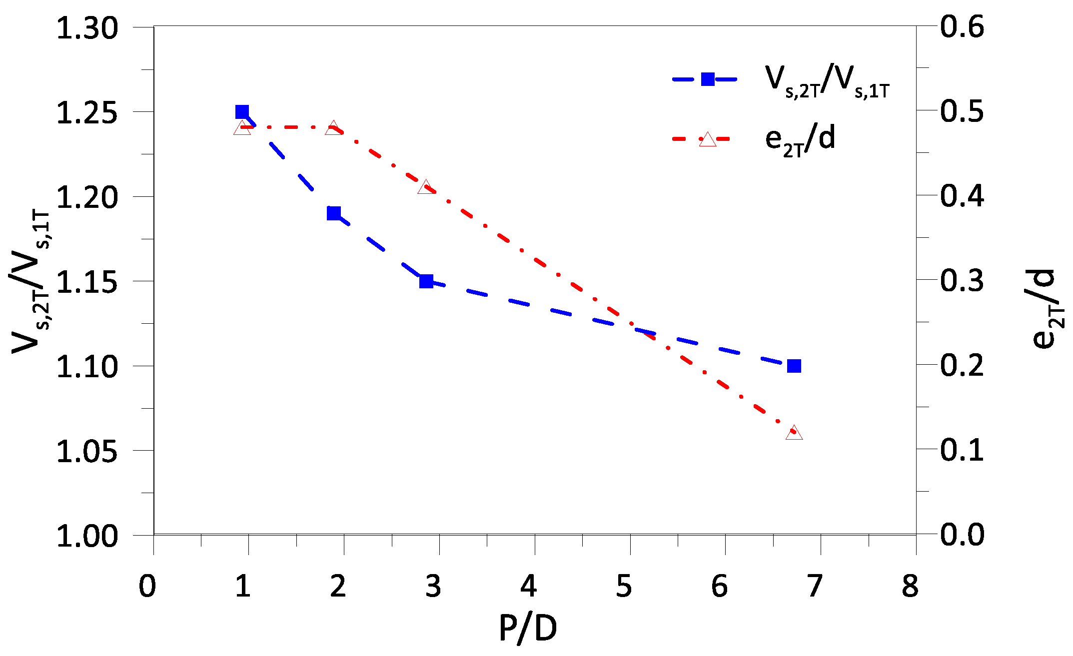
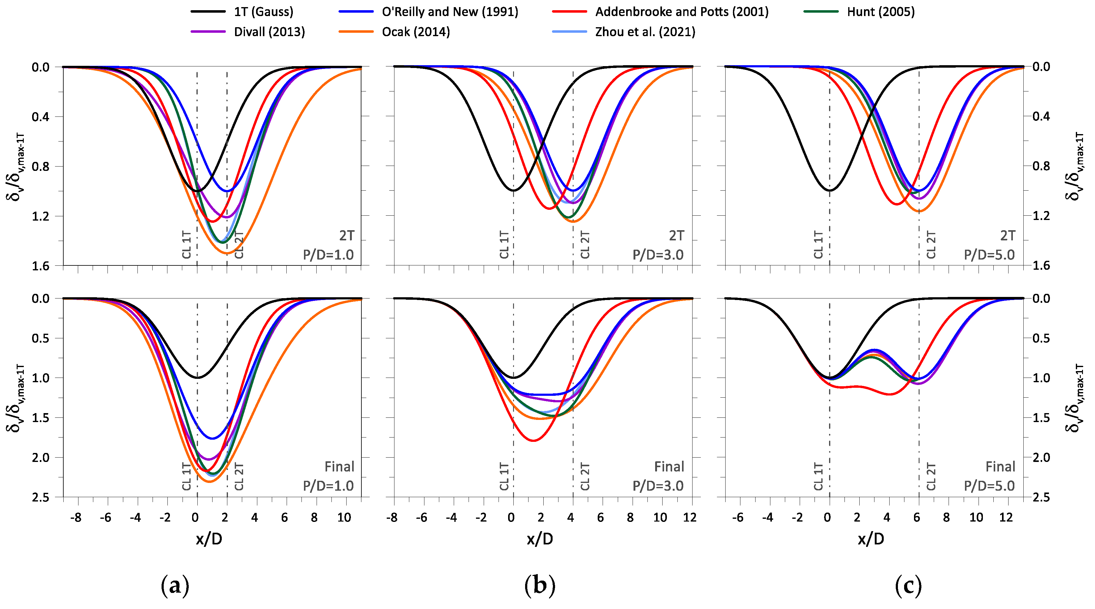
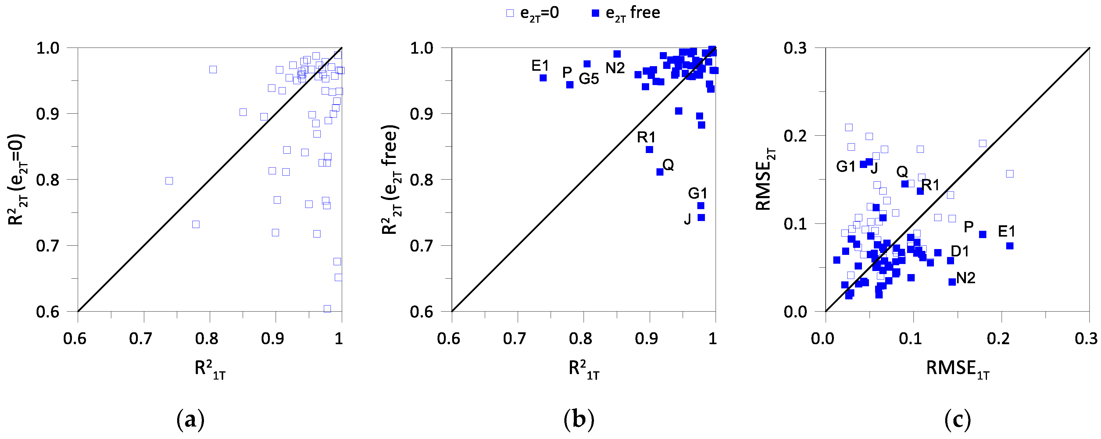
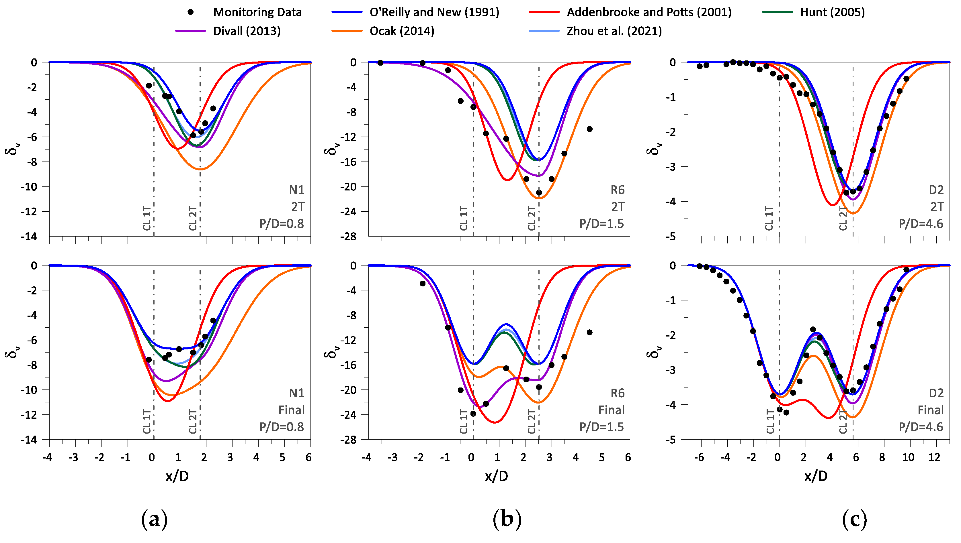
• All methods assume that the excavation of both the 1T and 2T induces a Gaussian settlement trough. With the exception of the O'Reilly and New [36] method, which does not account for tunnel interaction, all other methods predict that the 2T excavation induces higher settlements, with this increase being a function of the tunnels proximity;
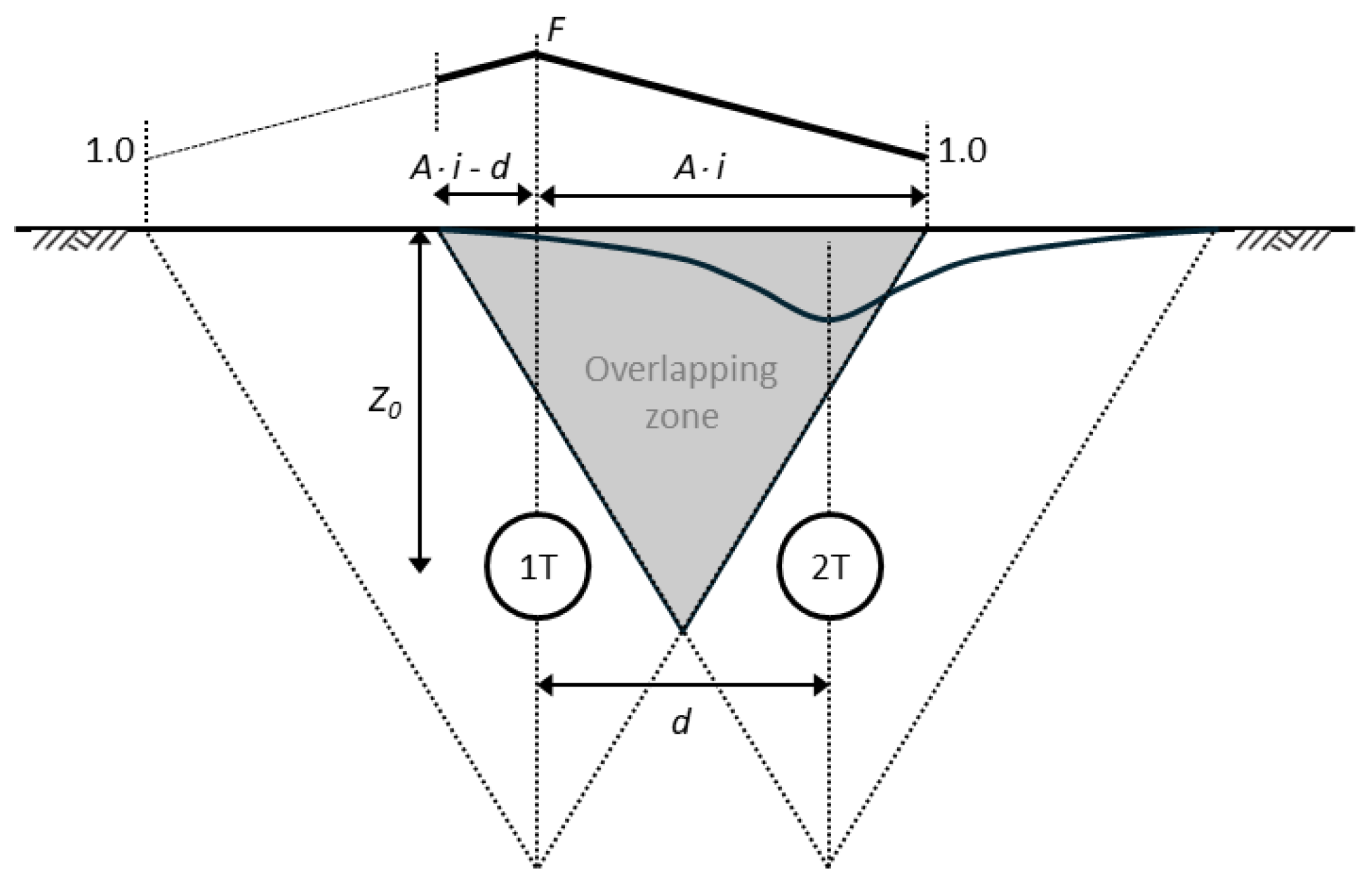
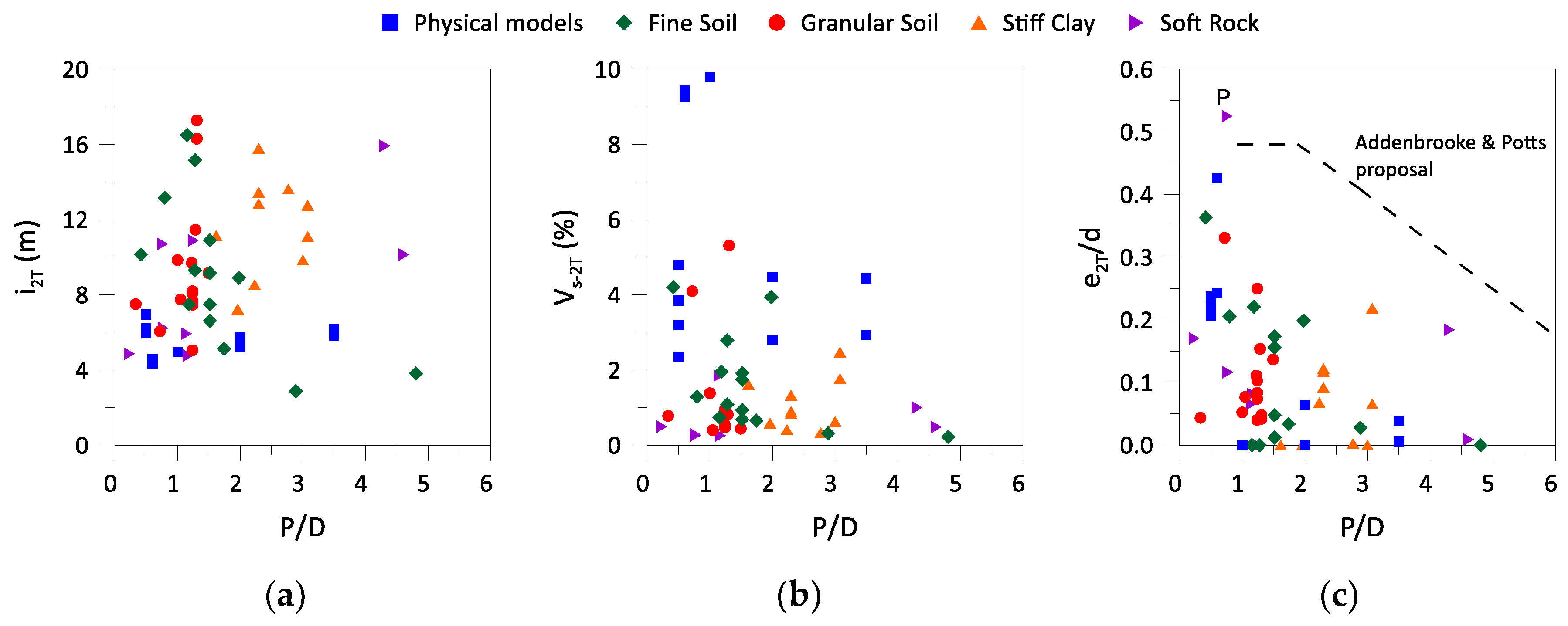
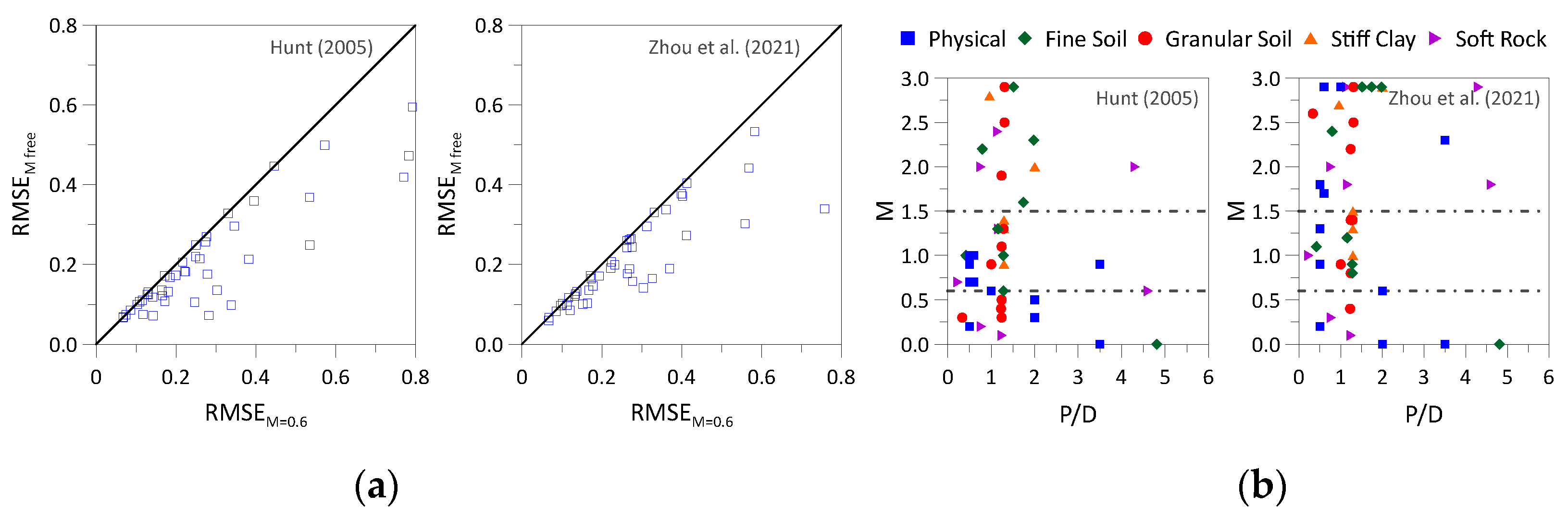
• The methods differ in how they account with the interaction effects: Addenbrooke and Potts [16] and Divall [43] suggest a correction for the volume loss (with an additional eccentricity correction in the case of the former); Hunt [39] and Zhou, et al. [38] propose the application of a corrective factor in the “overlapping zone” between both tunnels; and Ocak [37] suggests a correction factor applied to both the Gaussian parameters (maximum displacement and trough width);
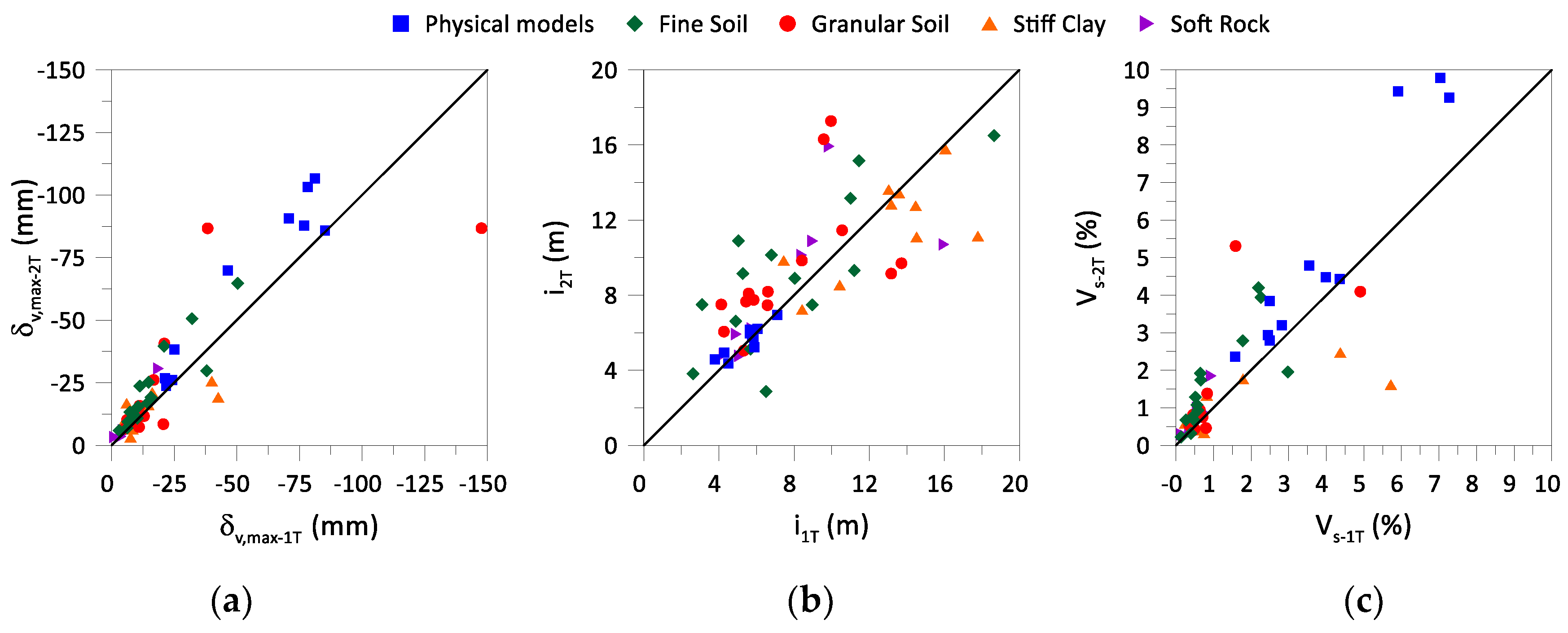
• The fitting of the monitoring data to the analyzed case studies confirmed that the settlements induced by the 1T are very adequately described by a Gaussian curve. However, for the settlements induced by the 2T a very good fit was only achieved if an eccentric Gaussian curve was considered. This confirms that the superposition method of two Gaussian curves is appropriate for predicting the settlements induced by twin tunnelling;
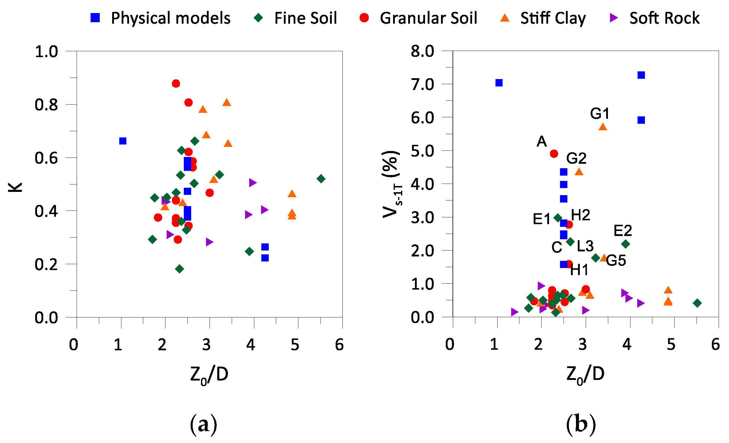
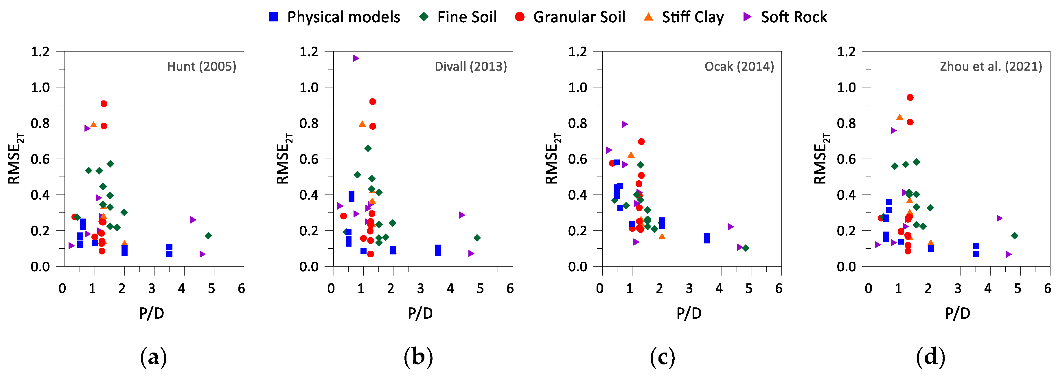
• Despite the very good fit the obtained Gaussian parameters exhibit significant scatter across all valid sections, and no clear trend was possible to establish in relation to either the soil type or the dimension of the pillar width;
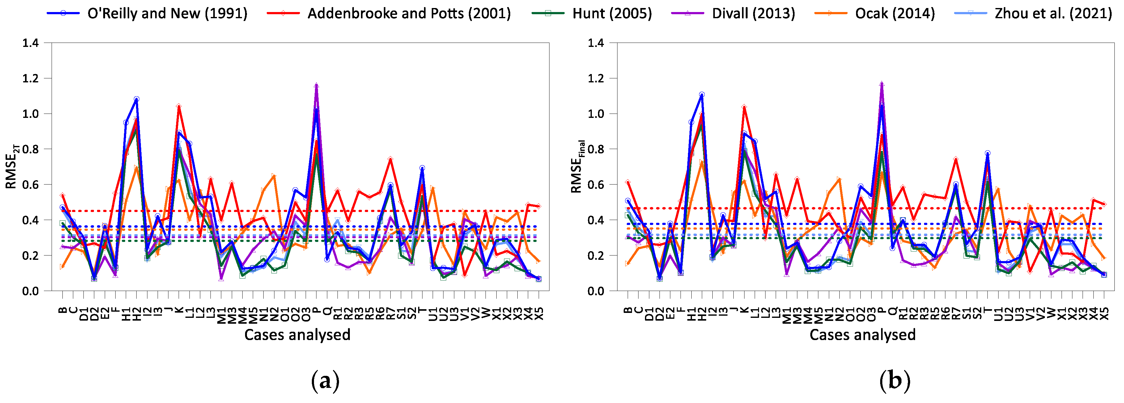
• The application of the analytical methods to predict the monitoring data revealed that the Addenbrooke and Potts [16] proposal performs very poorly due to the application of the eccentricity correction, performing even worse than O'Reilly and New [36] method. The remaining methods predict the induced settlements of the 2T excavation with similar accuracy, with Hunt [39] proposal being slightly more reliable across all cases, and regardless of the soil type or the dimension of the pillar width;
• The maximum modification parameter adopted by Hunt [39] and Zhou, et al. [38] methods to improve the 2T settlement prediction has a limited impact on the results, with improvements generally below 15%;

These results show that the existing analytical methods, with the exception of Addenbrooke and Potts [16] and O'Reilly and New [36] proposals, can be used to predict, with reasonably accuracy, the settlements associated to twin tunnelling during the early stages of design, across all ranges of soil types and P/D ratios. However, when tested against real case scenarios, all methods exhibited limitations that are inherent to the ground variability and the complexity associated with tunnel excavation process. Factors such as challenging ground conditions and inadequate operational shield parameters can induce substantial ground movements that cannot be predicted by simple analytical methods, which are only applicable to simple scenarios.

References

1. Admiraal, H.; Cornaro, A. Why underground space should be included in urban planning policy – And how this will enhance an urban underground future. Tunnelling and Underground Space Technology 2016, 55, 214–220. [Google Scholar] [CrossRef]
2. Bobylev, N. Underground space as an urban indicator: Measuring use of subsurface. Tunnelling and Underground Space Technology 2016, 55, 40–51. [Google Scholar] [CrossRef]
3. Broere, W. Urban underground space: Solving the problems of today’s cities. Tunnelling and Underground Space Technology 2016, 55, 245–248. [Google Scholar] [CrossRef]
4. Divall, S.; Goodey, R.J. Twin-tunnelling-induced ground movements in clay. Proceedings of the Institution of Civil Engineers - Geotechnical Engineering 2015, 168, 247–256. [Google Scholar] [CrossRef]
5. Islam, M.S.; Iskander, M. Twin tunnelling induced ground settlements: A review. Tunnelling and Underground Space Technology 2021, 110, 103614. [Google Scholar] [CrossRef]
6. Burland, J.B.; Standing, J.R.; Jardine, F.M. Assessing the risk of damage due to tunneling - lessons from the Jubilee Line Extension, London. In Proceedings of the 14th South-East Asian Conference on Geotechnical Engineering, Hong Kong, 2001; pp. 17-44.
7. Mair, R.J.; Taylor, R.N. Bored tunnelling in the urban environment. In Proceedings of the 14th International Conference on Soil Mechanics and Foundation Engineering, State-of-the-art Report and Theme Lecture, Hamburg, 1997; pp. 2353-2385.
8. Niu, G.; He, X.; Xu, H.; Dai, S. Tunnelling-induced ground surface settlement: A comprehensive review with particular attention to artificial intelligence technologies. Natural Hazards Research 2024, 4, 148–168. [Google Scholar] [CrossRef]
9. Peck, R.B. Deep excavations and tunnelling in soft ground. In Proceedings of the 7th International conference on soil mechanics and foundations engineering, Mexico City, 1969; pp. 225-290.
10. Cording, E.J.; Hansmire, W.H. Displacement around soft ground tunnels-General report. In Proceedings of the Proc. 5th Pan-American Conf. on Soil Mechanics and Foundation Engrg., Buenos Aires, 1975, 1975; pp. 571-632.
11. Perez Saiz, R.; Garami, J.; Arcones, A.; Soriano, A. Experience gained through tunnel instrumentation. In Proceedings of the Proceedings of the Tenth International Conference on Soil Mechanics and Foundation Engineering, Stockholm., 1981.
12. Fargnoli, V.; Boldini, D.; Amorosi, A. Twin tunnel excavation in coarse grained soils: Observations and numerical back-predictions under free field conditions and in presence of a surface structure. Tunnelling and Underground Space Technology 2015, 49, 454–469. [Google Scholar] [CrossRef]
13. Suwansawat, S.; Einstein, H.H. Describing Settlement Troughs over Twin Tunnels Using a Superposition Technique. Journal of Geotechnical and Geoenvironmental Engineering 2007, 133, 445–468. [Google Scholar] [CrossRef]
14. Ghaboussi, J.; Ranken, R.E. Interaction between two parallel tunnels. International Journal for Numerical and Analytical Methods in Geomechanics 1977, 1, 75–103. [Google Scholar] [CrossRef]
15. Soliman, E.; Duddeck, H.; Ahrens, H. Two- and three-dimensional analysis of closely spaced double-tube tunnels. Tunnelling and Underground Space Technology 1993, 8, 13–18. [Google Scholar] [CrossRef]
16. Addenbrooke, T.I.; Potts, D.M. Twin Tunnel Interaction: Surface and Subsurface Effects. International Journal of Geomechanics 2001, 1, 249–271. [Google Scholar] [CrossRef]
17. Ng, C.W.; Lee, K.M.; Tang, D.K. Three-dimensional numerical investigations of new Austrian tunnelling method (NATM) twin tunnel interactions. Canadian Geotechnical Journal 2004, 41, 523–539. [Google Scholar] [CrossRef]
18. Do, N.-A.; Dias, D.; Oreste, P.; Djeran-Maigre, I. Three-dimensional numerical simulation of a mechanized twin tunnels in soft ground. Tunnelling and Underground Space Technology 2014, 42, 40–51. [Google Scholar] [CrossRef]
19. Do, N.A.; Dias, D.; Oreste, P.; Djeran-Maigre, I. 2D numerical investigations of twin tunnel interaction. Geomech Eng 2014, 6, 263–275. [Google Scholar] [CrossRef]
20. Liu, H.Y.; Small, J.C.; Carter, J.P. Full 3D modelling for effects of tunnelling on existing support systems in the Sydney region. Tunnelling and Underground Space Technology 2008, 23, 399–420. [Google Scholar] [CrossRef]
21. Nematollahi, M.; Dias, D. Three-dimensional numerical simulation of pile-twin tunnels interaction – Case of the Shiraz subway line. Tunnelling and Underground Space Technology 2019, 86, 75–88. [Google Scholar] [CrossRef]
22. Chapman, D.N.; Rogers, C.D.F.; Hunt, D.V.L. Predicting the Settlements above Twin Tunnels Constructed in Soft Ground. In Proceedings of the 30th ITA-AITES world tunnel congess; 2002; p. 8. [Google Scholar]
23. Pedro, A.M.G.; Cancela, T.; Almeida e Sousa, J.; Grazina, J. Deformations caused by the excavation of twin tunnels. In Proceedings of the 9th Int. Symp. on Geot. Aspects of Underground Const. in Soft Ground, Sao Paulo, Brazil, 2017; pp. 203-213.
24. Miliziano, S.; Caponi, S.; Carlaccini, D.; de Lillis, A. Prediction of tunnelling-induced effects on a historic building in Rome. Tunnelling and Underground Space Technology 2022, 119, 104212. [Google Scholar] [CrossRef]
25. Chapman, D.N.; Ahn, S.K.; Hunt, D.V. Investigating ground movements caused by the construction of multiple tunnels in soft ground using laboratory model tests. Canadian Geotechnical Journal 2007, 44, 631–643. [Google Scholar] [CrossRef]
26. Divall, S.; Goodey, R.J.; Taylor, R.N. Ground movements generated by sequential twin-tunnelling in over-consolidated clay. In Proceedings of the 2nd European Conference on Physical Modelling in Geotechnics, Delft, Netherlands, 2012; p. 10.
27. He, C.; Feng, K.; Fang, Y.; Jiang, Y.-c. Surface settlement caused by twin-parallel shield tunnelling in sandy cobble strata. Journal of Zhejiang University SCIENCE A 2012, 13, 858–869. [Google Scholar] [CrossRef]
28. Zheng, G.; Tong, J.; Zhang, T.; Wang, R.; Fan, Q.; Sun, J.; Diao, Y. Experimental study on surface settlements induced by sequential excavation of two parallel tunnels in drained granular soil. Tunnelling and Underground Space Technology 2020, 98, 103347. [Google Scholar] [CrossRef]
29. Vlachopoulos, N.; Vazaios, I.; Madjdabadi, B.M. Investigation into the influence of excavation of twin-bored tunnels within weak rock masses adjacent to slopes. Canadian Geotechnical Journal 2018, 55, 1533–1551. [Google Scholar] [CrossRef]
30. Pedro, A.; Grazina, J.; Almeida e Sousa, J. Lining forces in tunnel interaction problems. Soils and Rocks 2022, 45, 1–12. [Google Scholar] [CrossRef]
31. Shivaei, S.; Hataf, N.; Pirastehfar, K. 3D numerical investigation of the coupled interaction behavior between mechanized twin tunnels and groundwater – A case study: Shiraz metro line 2. Tunnelling and Underground Space Technology 2020, 103, 103458. [Google Scholar] [CrossRef]
32. Sahoo, J.P.; Kumar, J. Required Lining Pressure for the Stability of Twin Circular Tunnels in Soils. International Journal of Geomechanics 2018, 18, 04018069. [Google Scholar] [CrossRef]
33. Yang, F.; Zheng, X.; Zhang, J.; Yang, J. Upper bound analysis of stability of dual circular tunnels subjected to surcharge loading in cohesive-frictional soils. Tunnelling and Underground Space Technology 2017, 61, 150–160. [Google Scholar] [CrossRef]
34. Pedro, A.M.G.; Grazina, J.C.; Almeida e Sousa, J. Stress redistribution in the central pillar between twin tunnels. In Proceedings of the NUMGE18, Porto, Portugal, 2018; pp. 1309-1317.
35. Zhang, T.; Taylor, R.N.; Divall, S.; Zheng, G.; Sun, J.; Stallebrass, S.E.; Goodey, R.J. Explanation for twin tunnelling-induced surface settlements by changes in soil stiffness on account of stress history. Tunnelling and Underground Space Technology 2019, 85, 160–169. [Google Scholar] [CrossRef]
36. O'Reilly, M.P.; New, B.M. Settlements above tunnel in the United Kingdom - their magnitude and prediction. In Proceedings of the Conference Tunnelling ’82, London, 1982; pp. 173 -181.
37. Ocak, I. A new approach for estimating the transverse surface settlement curve for twin tunnels in shallow and soft soils. Environmental Earth Sciences 2014, 72, 2357–2367. [Google Scholar] [CrossRef]
38. Zhou, Z.; Ding, H.; Miao, L.; Gong, C. Predictive model for the surface settlement caused by the excavation of twin tunnels. Tunnelling and Underground Space Technology 2021, 114, 104014. [Google Scholar] [CrossRef]
39. Hunt, D.V.L. Predicting the ground movements above twin tunnels constructed in London Clay. PhD thesis, University of Birmingham, Birmingham, 2005.
40. Dong, C.; Lin, J.; Cao, G.; Cheng, H.; Shi, L.; Zhang, X. Analytical Study on Surface Settlement Troughs Induced by the Sequential Excavation of Adjacent and Parallel Tunnels in Layered Soils. Advances in Civil Engineering 2022, 2022, 2489711. [Google Scholar] [CrossRef]
41. Mooney, M.; Grasmick, J.; Clemmensen, A.; Thompson, A.; Prantil, E.; Robinson, B. Ground deformation from multiple tunnel openings: analysis of Queens Bored Tunnels. Proc. North American Tunneling, Los Angeles, CA 2014.
42. Pedro, A.M.G.; Grazina, J.C.D.; Sousa, J.A.e. Influence of the pillar width on the construction sequence of twin tunnels. In Proceedings of the NUMGE23 - 10th European Conference on Numerical Methods in Geotechnical Engineering, London, UK, 2023.
43. Divall, S. Ground movements associated with twin-tunnel construction in clay. PhD thesis, City University London, London, 2013.
44. Wan, M.S.P.; Standing, J.R.; Potts, D.M.; Burland, J.B. Measured short-term ground surface response to EPBM tunnelling in London Clay. Géotechnique 2017, 67, 420–445. [Google Scholar] [CrossRef]
45. Ou, C.-Y.; Hwang, R.N.; Lai, W.-J. Surface settlement during shield tunnelling at CH218 in Taipei. Canadian Geotechnical Journal 1998, 35, 159–168. [Google Scholar] [CrossRef]
46. Withers, A.D. Chapter 37 - Surface displacements at three surface reference sites above twin tunnels through the Lambeth Group. In Building response to tunnelling; 2001; pp. 735-754.
47. Wu, B.R.; Lee, C.J. Ground movements and collapse mechanisms induced by tunneling in clayey soil. International Journal of Physical Modelling in Geotechnics 2003, 3, 15–29. [Google Scholar] [CrossRef]
48. Clayton, C.; Van Der Berg, J.; Thomas, A. Monitoring and displacements at Heathrow Express Terminal 4 station tunnels. Géotechnique 2006, 56, 323–334. [Google Scholar] [CrossRef]
49. Mahmutoğlu, Y. Surface subsidence induced by twin subway tunnelling in soft ground conditions in Istanbul. Bulletin of Engineering Geology and the Environment 2011, 70, 115–131. [Google Scholar] [CrossRef]
50. Bilotta, E.; Russo, G. Ground movements induced by tunnel boring in Naples. In Proceedings of the 2012 Proceedings of the 7th international symposium on geotechnical aspects of underground construction in soft ground, London, 2012.
51. Standing, J.R.; Selemetas, D. Greenfield ground response to EPBM tunnelling in London Clay. Géotechnique 2013, 63, 989–1007. [Google Scholar] [CrossRef]
52. Elwood, D.E.Y.; Martin, C.D. Ground response of closely spaced twin tunnels constructed in heavily overconsolidated soils. Tunnelling and Underground Space Technology 2016, 51, 226–237. [Google Scholar] [CrossRef]
53. Zhong, Z.; Li, C.; Liu, X.; Fan, Y.; Liang, N. Analysis of ground surface settlement induced by the construction of mechanized twin tunnels in soil-rock mass mixed ground. Tunnelling and Underground Space Technology 2021, 110, 103746. [Google Scholar] [CrossRef]
54. Kannangara, K.K.P.M.; Ding, Z.; Zhou, W.-H. Surface settlements induced by twin tunneling in silty sand. Underground Space 2022, 7, 58–75. [Google Scholar] [CrossRef]
55. Hu, Y.; Tang, H.; Xu, Y.; Lei, H.; Zeng, P.; Yao, K.; Dong, Y. Ground settlement and tunnel response due to twin-curved shield tunnelling in soft ground with small clear distance. Journal of Rock Mechanics and Geotechnical Engineering 2024, 16, 3122–3135. [Google Scholar] [CrossRef]
56. Divall, S.; Goodey, R.J.; Stallebrass, S.E. Twin-tunnelling-induced changes to clay stiffness. Géotechnique 2017, 67, 906–913. [Google Scholar] [CrossRef]
57. Chen, S.L.; Gui, M.W.; Yang, M.C. Applicability of the principle of superposition in estimating ground surface settlement of twin- and quadruple-tube tunnels. Tunnelling and Underground Space Technology 2012, 28, 135–149. [Google Scholar] [CrossRef]
Figure 1. Design chart proposed by Addenbrooke and Potts [16] (replotted using the original data).
Preprints 143361 g001
Figure 2. Overlapping zone according with Hunt [39] (modified from Hunt [39]).
Preprints 143361 g002
Figure 3. Comparison of the analytical methods proposed for the prediction of settlements induced by the 2T excavation for different pillar widths: (a) P/D=1.0; (b) P/D=3.0; (c) P/D=5.0.
Preprints 143361 g003
Figure 4. Geometrical characteristics of the twin tunnels analyzed in the case studies.
Preprints 143361 g004
Figure 5. Metrics associated with the fitting of the Gaussian curves: (a) R2 with no eccentricity; (b) R2 with free eccentricity; (c) RMSE.
Preprints 143361 g005
Figure 6. Comparison of the fitted Gaussian parameters for the 1T and 2T: (a) δ v , m a x ; (b) i ; (c) V s .
Preprints 143361 g006
Figure 7. Influence of the depth of the tunnel axis on the 1T excavation: (a) trough width factor; (b) volume loss.
Preprints 143361 g007
Figure 8. Influence of the pillar width on the 2T excavation: (a) i ; (b) V s ; (c)  e / d .
Preprints 143361 g008
Figure 9. Assessment of the predictions made by the analytical methods for the analyzed cases: (a) 2T settlements; (b) final settlements.
Preprints 143361 g009
Figure 10. Assessment of the predictions made by the analytical methods as a function of P/D ratio: (a) Hunt [39]; (b) Divall [43]; (c) Ocak [37]; (d) Zhou, et al. [38].
Preprints 143361 g010
Figure 11. Influence of the maximum modification factor employed in Hunt [39] and Zhou, et al. [38] methods: (a) RMSE; (b) pillar width.
Preprints 143361 g011
Figure 12. Settlements predicted for the 2T by the analytical methods for three cases analysed (a) N1; (b) R6; (c) D2.
Preprints 143361 g012