Identification of Power Lines with Currents Varying Strongly with Changes in Nodal Powers in a Power System

1. Introduction

For each power line the allowable current (ampacity [1]) is specified. More precisely, the allowable current is the maximum continuous current that flows on the power line, or in other word, when a current is considered as a complex value, it is a maximum allowable magnitude of current on a power line. Many factors influence that value. Attention should be paid to the structure of the power line, operational conditions (especially voltages), and weather conditions. In [2] the maximum possible power flow (and, consequently, the current) on the power line is considered depending on the operational conditions. There are methods that allow determining the allowable currents for power lines depending on weather conditions [3].

There are no papers in which the changes of magnitudes of currents on individual branches due to changes in generation and loads (i.e. changes in nodal powers) are considered. Knowledge of the above-mentioned relationships allows answering the questions: “On which branches do currents flow, the magnitudes of which change the most with changes in nodal powers?”, “For which nodes are these changes in nodal powers observed?” For individual cases, it is relatively easy to answer this question based on measurements or calculations (e.g. power-flow calculation [4,5,6,7,8]). The answer is much more difficult when many operational states of PS must be taken into account.

In order to emphasize the importance of the problem indicated earlier, it can be noted that in addition to considering the Branch Current Magnitudes (BCMs) in terms of ampacity, these BCMs should also be considered in terms of the deviations of the nodal voltages (more precisely, the deviations of the magnitudes of these voltages) and the active power losses in the branches.

It should be noted that if, along with a change in some nodal power, the magnitude of the current on a branch increases, the voltage drop on this branch will change, or more precisely, the voltage drop magnitude on this branch will increase. The consequence is a change in the voltage magnitude at the end node of the branch, in particular it may be a decrease in this magnitude, which may result in its reduction below the assumed minimum value. Another effect of the increase in the current magnitude on the branch is the increase in active power losses in the branch.

The answers to the questions formulated earlier contain information useful for engineers planning the development of PS and also for dispatchers. In both cases, they will help draw attention to branch currents whose magnitudes may assume too high values due to the increase in the appropriate nodal powers. As a result, when planning the development of PS, modernization decisions may be made leading to an increase in the allowable currents for the relevant branches. However, in the case of dispatchers, more justified decisions can be made regarding operations whose realization will increase power quality and the safety, reliability and economic efficiency of PS.

It is easy to see that if for each branch, the PS nodes will be found, at which the nodal powers are noticeably related to the magnitude of current on the considered branch, then in fact the PS clustering [9] will be performed from the point of view of significant relationships between branch currents and nodal powers. It is also possible to cluster PS assuming that for each PS node a set of branches is found in which there are currents that are noticeably related to the nodal power at this node. It can be expected that in both indicated cases soft clustering [9] takes place.

The possibility of clustering PS is interesting for the analysis of this system.

The aim of the paper is to show how to analyze PS from the point of view of identification of the branches on which there flow currents with magnitudes that change strongly with changes in nodal powers.

That aim is achieved through:

• Developing an approach to planned analyses.
• Using the adopted approach, developing an original method allowing for:
  • identification of branches on which there flow currents with magnitudes that change strongly with changes in nodal powers,
  • for each of the previously-identified branches, finding a set of nodes with nodal powers whose changes are strongly related to change in the magnitude of current on the considered branch,
  • among the previously indicated branches, finding sets of branches, each of which includes branches with currents flowing on them having magnitudes whose changes are strongly related to changes in nodal power at the same node.
• Presentation of the use of the developed method in a case study in which IEEE 14-bus Test System (TS) is considered [10].
• Presentation of the properties of the proposed method.

2. Correlational Approach to Considered Identification

At any time, the energy delivered to PS should cover the consumers’ demand for electrical energy and the losses of this energy during its transmission from the place of generation to the place of its utilization. The individual loads and, as a result, the generation powers change over time. These changes cannot be determined deterministically. With changes in loads and generation powers (collectively called nodal powers), active and reactive power flows in PS and, consequently, currents on the PS branches change. In this situation, stochastic description can be used to describe phenomena in PS. To solve the problem, which is considered in the paper, i.e. finding strong relationships between BCMs and the Nodal Apparent Powers (NAPs) as well as strong relationships between BCMs and the Nodal Power Arguments (NPAs), Correlational Relationships (CRs) between the distinguished quantities can be used. CR simply says that two considered variables perform in a synchronized manner [11].

The correlation approach to solved problems in PS is used in other articles (e.g. [12,13,14,15,16,17,18,19]). However, no other paper has used this approach to solve a problem such as the one considered in this paper.

The investigations of CRs allows to determine the strength of the relationships between BCMs and NAPs as well as to determine the strength of the relationships between BCMs and NPAs. These investigations make it possible to identify the branches of PS on which currents are strongly related to nodal powers. Such a strong relationship means that when NAP or NPA change, there is a significant change in the considered BCM. In particular, an increase in NAP or NPA may result in an increase in BCM. The previously mentioned relationship may also mean a decrease in BCM with an increase in NAP or NPA. Stochastic investigation means that it is not enough to examine only the strength of CRs, but also the statistical significance of these relationships must be established. For the purposes of examining the relationships between BCMs and NAPs or between BCMs and NPAs, only Statistically Significant Correlational Relationships (SSCRs) should be taken into account.

3. Investigation of Correlational Relationships Between Distinguished Quantities

When examining CRs, it is important to determine the strength of association of the considered quantities. Various correlation coefficients are used as measures of this strength. The most well-known correlation coefficients are: (i) the Pearson product-moment correlation coefficient (Pearson’s correlation coefficient), (ii) the Spearman’s rank correlation coefficient (Spearman’s rho), (iii) the Kendall’s Rank Correlation Coefficient (KRCC) [20,21]. Further considerations are carried out to determine which of the correlation coefficients is the most appropriate.

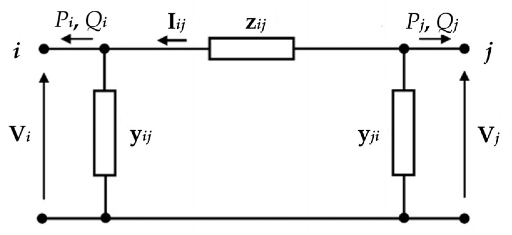
The current on a branch of PS can be determined as a result of measurement using a PMU device or it can be calculated on the basis of measurements of active and reactive power flows on the branch. The PMU device allows obtaining the current phasor, i.e. its magnitude and argument. For the purposes of the considerations given in the paper, it is necessary to know BCMs. If there is no measurement of the current phasor, but only measurements of active and reactive power flows, then the magnitude of branch current on branch b_{i_j}, i.e. a branch between nodes n_i and n_j, where n_i – a node in PS with number i, can be calculated from the formula:

$$I_{ij}={\displaystyle \frac{\sqrt{P_{ij}^2+Q_{ij}^2}}{V_i}},$$

(1)

where: I_ij – a magnitude of current on branch b_{i_j} at node n_i; P_ij, Q_ij – active and reactive power flows on branch b_{i_j} at node n_i, respectively; V_i – a magnitude of the voltage at node n_i.

Figure 1. The assumed Π model of power line b_{i_j}. z_ij = r_ij + j x_ij, y_ij = j 0.5 b_ij, y_ji = j 0.5 b_ij.

Figure 1. The assumed Π model of power line b_{i_j}. z_ij = r_ij + j x_ij, y_ij = j 0.5 b_ij, y_ji = j 0.5 b_ij.

Power flows P_ij and Q_ij are related to the nodal voltages V_i, V_j:

$$P_{ij}=\mathrm{R}\mathrm{e}{\mathbf{S}}_{ij}, Q_{ij}=\mathrm{I}\mathrm{m}{\mathbf{S}}_{ij},$$

(2)

where ${\mathbf{S}}_{ij}$ – a complex power flow on branch b_{i_j} at end i:

$${\mathbf{S}}_{ij}={\mathbf{V}}_i{\mathbf{I}}_{ij}^{\mathit{*}}={\mathbf{V}}_i{\mathbf{V}}_j^{\mathit{*}}/{\mathbf{z}}_{ij}^{\mathit{*}}-V_i^2\left(1/{\mathbf{z}}_{ij}^{\mathit{*}}+{\mathrm{y}}_{ij}^{*}\right).$$

(3)

Power flows P_ji and Q_ji are given by the formulas

$$P_{ji}=\mathrm{R}\mathrm{e} {\mathbf{S}}_{ji},Q_{ji}=\mathrm{I}\mathrm{m} {\mathbf{S}}_{ji},$$

(4)

where ${\mathbf{S}}_{ji}$ – complex power flows on branch b_{j_i} at end j:

$${\mathbf{S}}_{ji}={\mathbf{V}}_j{\mathbf{I}}_{ji}^{\mathit{*}}={\mathbf{V}}_j{\mathbf{V}}_i^{\mathit{*}}/{\mathbf{z}}_{ij}^{\mathit{*}}-V_j^2\left(1/{\mathbf{z}}_{ij}^{\mathit{*}}+{\mathit{y}}_{ji}^{*}\right).$$

(5)

Based on (2) and (4), it can be concluded that, in general:

$$P_{ij}\ne P_{ji},Q_{ij}\ne Q_{ji}.$$

(6)

Also, if any of the active or reactive power flows is different from zero, then (see Appendix A in [13])

$$V_i\ne V_j.$$

(7)

In consequence

$$I_{ij}\ne I_{ji}.$$

(8)

Nodal voltages in PS depend on the nodal active and reactive powers, or in other words, on the nodal complex powers.

A conjugate complex power for node n_k k ∈ {1, 2, …, n}, where n – a number of nodes in PS, is as follows:

$${\mathbf{S}}_k^{*}=P_k-\mathrm{j}{Q}_k={\mathbf{V}}_k^{*}{\sum }_{l=1}^n{\mathbf{Y}}_{kl}{\mathbf{V}}_{\mathit{l}},$$

(9)

where P_k, Q_k – a nodal active and reactive powers, respectively; Y_kl – an element of the admittance matrix.

The magnitude and argument of the k-th complex nodal power can be calculated from the formulas:

$$S_k=\sqrt{P_k^2+Q_k^2},$$

(10)

$${\mathsf{\phi }}_k=\mathrm{a}\mathrm{r}\mathrm{c}\mathrm{t}\mathrm{a}\mathrm{n}\left(Q_k/P_k\right).$$

(11)

The presented considerations indicate that the relationship between BCM I_ij and NAP S_k as well as between BCM I_ij and NPA φ_k is non-linear. According to [20,21], the appropriate measure for assessing CRs between BCMs and NAPs or CRs between BCMs and NPAs is KRCC.

For the aim of interpreting the size of KRCC, which characterizes each of the considered CR, the same rule of thumb as in [14] is taken into account (Table 1).

Hereafter, (i) cr_U-W stands for CR between U and W, (ii) t_k,U-W stands for KRCC characterizing CR between quantities U and W.

4. Proposed Method

• Step 0

1.

Creation of data sets of magnitudes of individual currents at the ends of the PS branches:

• if current phasors are measured at the ends of the branches of PS, then elements of the sets of observations of BCMs are measurements of BCMs,
• if active and reactive power flows are measured at the ends of the branches of PS, then elements of the set of observations of BCMs are results of calculations using formula (1).

2.

Creation of data sets of NAPs and NPAs, calculated on the basis of active and reactive nodal powers in accordance with formulas (10), (11), respectively.

• Step 1

1.

Analyzes of CRs between BCMs and NAPs.

• Calculation of KRCCs for CRs between magnitudes of the currents at the ends of the PS branches and NAPs.
  For each branch, among the two CRs between the magnitudes of currents at the branch ends and NAP S_k k ∈ {1, 2, …, n}, select CR for which the absolute value of KRCC is larger. The selected CR is the characteristic CR between the magnitude of current on the considered branch and NAP S_k k ∈ {1, 2, …, n}.
• Creating set $S_{\mathrm{I}-\mathrm{S}}^x$, the elements of which are characteristic CRs between BCMs and NAPs, and the set of possessed data (used for calculation of KRCC) meets the conditions such as number of data and range of PS active power losses, for which the data are determined.

Hereinafter, an instance of a data set meeting the above conditions is called Case x. x is determined depending on the number of the data and the range of values of PS active power losses, which were mentioned earlier.

The following operations, which are required by the method, are presented only for one Case x. The method assumes performing the same operations for each considered Case x.

2.

Analyzes of CRs between BCMs and NPAs.

• Calculation of KRCCs for CRs between magnitudes of the currents at the ends of PS branches and NPAs.
  For each branch, among the two CRs between the magnitudes of currents at the branch ends and NPA φ_k k ∈ {1, 2, …, n}, select CR for which the absolute value of KRCC is larger. The selected CR is the characteristic CR between the magnitude of the current on the considered branch and NPA φ_k k ∈ {1, 2, …, n}.
• Creating set $S_{\mathrm{I}-\mathsf{\phi }}^x$, the elements of which are characteristic CRs between BCMs and NPAs.

• Step 2

• Performing significance tests of all CRs from set $S_{\mathrm{I}-\mathrm{S}}^x$.

In each of such significance tests the following statistic is used [20]:

$$z={\displaystyle \frac{3t_{k,U-W}\sqrt{m\left(m-1\right)}}{\sqrt{2\left(2m+5\right)}}},$$

(12)

where U, W – variables occurring in considered CR, i.e. BCM and NAP, respectively; m - a number of observations (data) of each of variables between which the correlation is examined.

The statistic z is approximately distributed as a standard normal under assumption, that considered variables are statistically independent.

2.

Creating ordered set $S_{\mathrm{S},\mathrm{I}-\mathrm{S}}^x$, the elements of which are SSCRs between BCMs and NAPs and these CRs are elements of set $S_{\mathrm{I}-\mathrm{S}}^x$.

The elements of set $S_{\mathrm{S},\mathrm{I}-\mathrm{S}}^x$ are arranged in the order of decreasing KRCCs, characterizing the individual CRs.

3.

Performing significance tests of all CRs from set $S_{\mathrm{I}-\mathsf{\phi }}^x$, using the statistic (12).

4.

Creating ordered set $S_{\mathrm{S},\mathrm{I}-\mathsf{\phi }}^x$, the elements of which are SSCRs between BCMs and NPAs and these CRs are elements of set $S_{\mathrm{I}-\mathsf{\phi }}^x$ for Case x.

The ordering criterion for set $S_{\mathrm{S},\mathrm{I}-\mathsf{\phi }}^x$ is the same as for set $S_{\mathrm{S},\mathrm{I}-\mathrm{S}}^x$.

• Step 3

Creating sets $S_{\mathrm{S},\mathrm{I}-\mathrm{S}}^{x,range}$ and $S_{\mathrm{S},\mathrm{I}-\mathsf{\phi }}^{x,range}$, being subsets of sets $S_{\mathrm{S},\mathrm{I}-\mathrm{S}}^x$ and $S_{\mathrm{S},\mathrm{I}-\mathsf{\phi }}^x$, respectively. For each element of set $S_{\mathrm{S},\mathrm{I}-\mathrm{S}}^{x,range}$ and for each element of set $S_{\mathrm{S},\mathrm{I}-\mathsf{\phi }}^{x,range}$ the absolute value of KRCC is in range range.

• Step 4

• Creating ordered set $A_{\mathrm{B}}^{x,\mathrm{r}\mathrm{a}\mathrm{n}\mathrm{g}\mathrm{e}}$ containing branches, each of which is characterized by the fact that the current flowing on it has magnitude that is in SSCRs belonging to set $S_{\mathrm{S},\mathrm{I}\_\mathrm{S}}^{x,range}$ or set $S_{\mathrm{S},\mathrm{I}\_\mathsf{\phi }}^{x,range}$.
  The branches in set $A_{\mathrm{B}}^{x,range}$ are arranged in` decreasing order of the absolute values of KRCCs for CRs between BCMs and NAPs or for CRs between BCMs and NPAs. The branch that is in the first position is the one on which there is current with the magnitude remaining in the strongest CR with a specific NAP or a specific NPA. One branch appears only once in set $A_{\mathrm{B}}^{x,range}$. The position of a branch in set $A_{\mathrm{B}}^{x,range}$ is determined by the maximal value of the absolute values of KRCCs for the CRs between BCM and the NAPs as well as for the CRs between BCM and the NPAs.
• Creating ordered set $A_{\mathrm{N}}^{x,range}$, containing nodes, each of which is characterized by the fact that NAP at this node is in SSCRs belonging to set $S_{\mathrm{S},\mathrm{I}\_\mathrm{S}}^{x,range}$ or NPA at this node is in SSCRs belonging to set $S_{\mathrm{S},\mathrm{I}\_\mathsf{\phi }}^{x,range}$.
  The nodes in set $A_{\mathrm{N}}^{x,range}$ are arranged in decreasing order of the absolute values of KRCCs for considered CRs The larger the position number of a node, the weaker the correlation between NAP or NPA at this node and the corresponding BCM. A node appears only once in set $A_{\mathrm{N}}^{x,range}$ at a position that is defined by the maximum value of the absolute values of KRCCs for CRs between NAP at that node and the BCMs as well as for CRs between NPA at that node and the BCMs.

• Step 5

• For each BCM I_ij i, j ∈ {1,2,…,n}, i ≠ j, creating sets $A_{\mathrm{S}\mathrm{F}\_\mathrm{Y},Iij}^x$ Y = S, φ, i.e. a set of NAPs being in SSCRs with BCM I_ij and a set of NPAs being in SSCRs with BCM I_ij, respectively, in Case x. Set $A_{\mathrm{S}\mathrm{F}\_\mathrm{Y},Iij}^x$ Y ∈ {S, φ} is associated with BCM I_ij and it is called as the set of influence factors $A_{\mathrm{S}\mathrm{F}\_\mathrm{Y},Iij}^x$ associated with BCM I_ij.

Hereinafter: $A_{\mathrm{S}\mathrm{F}\_\mathrm{S}}^{\mathrm{x}}$ and $A_{\mathrm{S}\mathrm{F}\_\mathsf{\phi }}^x$ are sets of all sets $A_{\mathrm{S}\mathrm{F}\_\mathrm{S},Iij}^x$ and $A_{\mathrm{S}\mathrm{F}\_\mathsf{\phi },Iij}^x$, respectively, where i, j ∈ {1,2,…,n}, i ≠ j.

2.

For each Y_k, where Y_k∈ {S_k, φ_k} k ∈ {1, 2, …, n}, creating set $A_{\mathrm{S},Yk}^x$, which is a set of BCMs being in SSCRs with quantity Y_k in Case x. Set $A_{\mathrm{S},Yk}^x$ is associated with quantity Y_k and it is called as the influence set associated with the quantity Y_k. The term “influence set” is used in [14]. In the paper, the definition of that term is adapted to the problem, which is considered here.

Hereinafter: $A_{\mathrm{S},\mathrm{S}}^x$ = $\left\{A_{\mathrm{S},S1}^x,A_{\mathrm{S},S2}^x,\dots ,A_{\mathrm{S},S14}^x\right\}$ and $A_{\mathrm{S},\mathsf{\phi }}^x$ = $\left\{A_{\mathrm{S},\mathsf{\phi }1}^x,A_{\mathrm{S},\mathsf{\phi }2}^x,\dots ,A_{\mathrm{S},\mathsf{\phi }14}^x\right\}$.

• Step 6

• For each BCM I_ij, creating sets $A_{\mathrm{S}\mathrm{F}\_Y,Iij}^{\mathrm{x},range}$ Y = S, φ, i, j ∈ {1, 2,…, n}, i ≠ j i.e. a subset of $A_{\mathrm{S}\mathrm{F}\_\mathrm{S},Iij}^x$ i, j ∈ {1, 2,…, n}, i ≠ j, which contains NAPs being in SSCRs with BCM I_ij and a subset of $A_{\mathrm{S}\mathrm{F}\_\mathsf{\phi },Iij}^x$ i, j ∈ {1, 2,…, n}, i ≠ j which contains NPAs being in SSCRs with BCM I_ij and the mentioned SSCRs are characterized by KRCCs from range range.
• For each Y_k, where Y_k∈ {S_k, φ_k} k ∈ {1, 2, …, n}, creating set $A_{\mathrm{S},Yk}^{x,range}$, i.e. a subset of $A_{\mathrm{S},Yk}^x$, which contains BCMs being in SSCRs with quantity Y_k, under assumption that for each of the SSCRs, KRCC is from range range.

Hereinafter: $A_{\mathrm{S},S}^{x,range}$ = $\left\{A_{\mathrm{S},S1}^{x,range},A_{\mathrm{S},S2}^{x,range},\dots ,A_{\mathrm{S},Sn}^{x,range}\right\}$ and

$A_{\mathrm{S},\mathsf{\phi }}^{x,range}$ = $\left\{A_{\mathrm{S},\mathsf{\phi }1}^{x,range},A_{\mathrm{S},\mathsf{\phi }2}^{x,range},\dots ,A_{\mathrm{S},\mathsf{\phi }n}^{x,range}\right\}$

• Step 7

• Creating set $A_{\mathrm{S}\mathrm{F},\mathrm{B}}^{x,range}$ containing branches b_{i_j} i, j ∈ {1, 2,…, n}, i ≠ j on which currents have magnitudes being in SSCRs with NAPs from set $A_{\mathrm{S}\mathrm{F}\_\mathrm{S},Iij}^{\mathrm{x},range}$ (i.e. $\left|A_{\mathrm{S}\mathrm{F}\_\mathrm{S},Iij}^{x,range}\right|>0$) or in SSCRs with NPAs from set $A_{\mathrm{S}\mathrm{F}\_\mathsf{\phi },Iij}^{x,,range}$, (i.e. $\left|A_{\mathrm{S}\mathrm{F}\_\mathsf{\phi },Iij}^{x,range}\right|>0$) ordered using coefficient
  $t_{\mathrm{k},\mathrm{S}\mathrm{F},Iij,\left|\right|,\mathrm{m}}^{x,range}=\max \left(t_{\mathrm{k},\mathrm{S}\mathrm{F}\_\mathrm{S},Iij,\left|\right|,\mathrm{m}}^{x,range}, t_{\mathrm{k},\mathrm{S}\mathrm{F}\_\mathsf{\phi },Iij,\left|\right|,\mathrm{m}}^{x,range}\right)$ i, j ∈ {1, 2,…, n}, i ≠ j.

Hereinafter, $t_{\mathrm{k},\mathrm{S}\mathrm{F}\_Y,Iij,\left|\right|,\mathrm{m}}^{x,range}$ will stand for average values of absolute values of KRCCs of SSCRs between quantities being elements of set $A_{\mathrm{S}\mathrm{F}\_Y,Iij}^{x,range}$, Y ∈ {S, φ}, i, j ∈ {1,2,…,n}, i ≠ j and BCM, with which this set is associated.

For subsequent items in set $A_{\mathrm{S}\mathrm{F},\mathrm{B}}^{x,range}$, index $t_{\mathrm{k},\mathrm{S}\mathrm{F},Iij,\left|\right|,\mathrm{m}}^{x,range}$ is smaller and smaller.

When determining the elements of set $A_{\mathrm{S}\mathrm{F},\mathrm{B}}^{x,range}$, the following assumptions are made: (i) set $A_{\mathrm{S}\mathrm{F}\_\mathrm{S},Iij}^{\mathrm{x},range}$ as well as $A_{\mathrm{S}\mathrm{F}\_\mathsf{\phi },Iij}^{x,,range}$, whose cardinality is greater than 1 is taken into account, (ii) if $\left|A_{\mathrm{S}\mathrm{F}\_\mathrm{S},Iij}^{\mathrm{x},range}\right|\le 1$ then $t_{\mathrm{k},\mathrm{S}\mathrm{F}\_\mathrm{S},Iij,\left|\right|,\mathrm{m}}^{x,range}=0$, (iii) if $\left|A_{\mathrm{S}\mathrm{F}\_\mathsf{\phi },Iij}^{\mathrm{x},range}\right|\le 1$ then $t_{\mathrm{k},\mathrm{S}\mathrm{F}\_\mathsf{\phi },Iij,\left|\right|,\mathrm{m}}^{x,range}=0$.

2.

Creating ordered set $A_{\mathrm{S},\mathrm{N}}^{x, range}$ containing nodes n_k k ∈ {1, 2, …, n}, each of which satisfies the condition that either NAP or NPA at it is in SSCRs with BCMs from set $A_{\mathrm{S},Sk}^{x,range}$ or $A_{\mathrm{S},\mathsf{\phi }k}^{x,range}$, respectively.

The nodes in set $A_{\mathrm{S},\mathrm{N}}^{x, range}$ are ordered in decreasing order of values of the following coefficient: $t_{\mathrm{k},\mathrm{S},k,\left|\right|,\mathrm{m}}^{x,range}=\max \left(t_{\mathrm{k},\mathrm{S},Sk,\left|\right|,\mathrm{m}}^{x,range}, t_{\mathrm{k},\mathrm{S},\mathsf{\phi }k,\left|\right|,\mathrm{m}}^{x,range}\right)$.

Hereinafter, $t_{\mathrm{k},\mathrm{S},Yk,\left|\right|,\mathrm{m}}^{x,range}$ will stand for average values of absolute values of KRCCs of SSCRs between quantities being elements of set $A_{\mathrm{S},Yk}^{x,range}$, Y_k∈ {S_k, φ_k}, k ∈ {1,2,…,n} and NAP or NPA, with which this set is associated.

Set $A_{\mathrm{S},\mathrm{N}}^{x, range}$ is created under assumptions: (i) set $A_{\mathrm{S},Sk}^{x,range}$ is taken into account, as well as set $A_{\mathrm{S},\mathsf{\phi }k}^{x,range}$, if it has cardinality greater than 1, (ii) if $\left|A_{\mathrm{S},Sk}^{\mathrm{x},range}\right|\le 1$ then $t_{\mathrm{k},\mathrm{S},Sk,\left|\right|,\mathrm{m}}^{x,range}=0$, (iii) if $\left|A_{\mathrm{S},\mathsf{\phi }k}^{\mathrm{x},range}\right|\le 1$ then $t_{\mathrm{k},\mathrm{S},\mathsf{\phi }k,\left|\right|,\mathrm{m}}^{x,range}=0$.

In Step 4, the following are found: 4.1) branches on which currents have magnitudes changing significantly with changes in NAPs or NPAs, 4.2) nodes at which powers have magnitudes or arguments that significantly affect BCMs. It should be added that, the number of earlier indicated branches as well as nodes is limited by constraints of the strength of CRs between BCMs and NAPs or CRs between BCMs and NPAs.

The result of searching for branches, on which currents have magnitudes changing strongly with changes in NAPs or NPAs, is set $A_{\mathrm{B}}^{x,\mathrm{r}\mathrm{a}\mathrm{n}\mathrm{g}\mathrm{e}}$ (Step 4.1). The previous statement is correct under assumption that range range includes the KRCC values characterizing strong CR. This assumption is made later in this section. For each of the mentioned branches, changes of BCM are when there are changes in NAP or NPA at at least one node. The nodes, at which there are NAP or NPA being in strong CRs with BCMs are in $A_{\mathrm{N}}^{x,\mathrm{r}\mathrm{a}\mathrm{n}\mathrm{g}\mathrm{e}}$ (Step 4.2). An analogous remark to that which applies to branches from set $A_{\mathrm{B}}^{x,\mathrm{r}\mathrm{a}\mathrm{n}\mathrm{g}\mathrm{e}}$ also applies to nodes from set $A_{\mathrm{N}}^{x,\mathrm{r}\mathrm{a}\mathrm{n}\mathrm{g}\mathrm{e}}$. Each node from set $A_{\mathrm{N}}^{x,\mathrm{r}\mathrm{a}\mathrm{n}\mathrm{g}\mathrm{e}}$ is associated with a NAP or NPA which is in at least one SSCR with the BCM.

Branches, on which there are currents with magnitudes changing strongly with changes of NAP or NPA at two or more nodes, are elements of set $A_{\mathrm{S}\mathrm{F},\mathrm{B}}^{x,range}$ (Step 7.1). In turn, nodes, at which there are NAPs or NPAs entering strong CRs with at least two branches, are in set $A_{\mathrm{S},\mathrm{N}}^{x, range}$ (Step 7.2).

Step 5 provides different information than Step 2. Whereas Step 2 shows CRs, each of which is an association of one BCM with one NAP or one NPA, Step 5 indicates: 5.1) at least one NAP or at least one NPA for one BCM, 5.2) at least one BCM for one NAP or one NPA. In step 6, the following are limited: 6.1) the numbers of NAPs or NPAs determined in step 5.1, 6.2) the numbers of BCMs determined in step 5.2, by imposing constraints on the strengths of CRs between BCMs and NAPs or CRs between BCMs and NPAs.

It should be noted that the sets created in step 5 define clusters in the PS. These are: 5.1) clusters from the point of view of BCMs - each cluster includes nodes at which the nodal powers significantly affect the corresponding BCM, 5.2) clusters from the point of view of the influence of NAPs or NPAs on BCMs - each cluster includes branches on which there are the mentioned currents.

5. Case Study 1

The section presents the application of the previously described method that allows: (i) identifying branches on which there are currents whose magnitudes change the most with changes in nodal powers, (ii) identifying nodes, at which there are NAPs or NPAs strongly influencing BCMs, (iii) clustering of PS from the point of view of influence of NAPs on magnitudes of individual branch currents, (iv) clustering of PS from the point of view of influence of NPAs on magnitudes of individual branch currents, (v) clustering of PS from the point of view of the influence of individual NAPs on branch current magnitudes. For the purposes of the method, data from TS [10] are taken under consideration. States in TS are considered in which the system active-power losses are in the range [0.06, 0.34] pu. This is Case a (Case x, where x = a).

In the analyses, the relationships between BCMs and NAPs and between BCMs and NPA are taken into account separately. In each of these cases, taking into account characteristic CRs for branches, the number of all CRs is equal to 280 (number of nodes: 14, number of branches: 20). In Table 2, the numbers of SSCRs are shown as a percentage of the total numbers of CRs in the considered cases. Testing the statistical significance of CRs is performed under assumption that the significance level is equal to 0.01.

Table 3 and Table 4 show the data related to SSCRs, which are members of sets $S_{S, I-S}^{\mathrm{a}}$ and $S_{S,I-\mathsf{\phi }}^{\mathrm{a}}$, respectively.

Table 3 and Table 4 show data on the characteristic SSCRs (for branches) between BCMs and NAPs and data on the characteristic SSCRs between BCMs and NPAs, respectively. In both tables, for each pair of quantities between which there is an SSCR, the KRCC is given. In each of these tables, the data are arranged in the order of decreasing KRCC. In Table 3, the shaded parts contain data relating to SSCRs for which absolute values of KRCCs are not less than 0.5 and in Table 4, these shaded parts contain data relating to SSCRs for which absolute values of KRCCs are not less than 0.3.

Based on Table 3, it can be stated that:

$$\begin{gathered} S_{\mathrm{S},\mathrm{I}-\mathrm{S}}^{\mathrm{a},\left[0.5, 1\right]}=\{{cr}_{I7\_8-S8}, {cr}_{I2\_3-S3},{cr}_{I3\_4-S3}, {cr}_{I1\_2-S1},{cr}_{I1\_5-S1}, \\ {cr}_{I4\_5-S1}, {cr}_{I2\_3-S1}, {cr}_{I2\_4-S1},{cr}_{I6\_12-S12}, \}, \end{gathered}$$

(13)

$$\begin{gathered} S_{\mathrm{S},\mathrm{I}-\mathrm{S}}^{\mathrm{a},\left[0.3, 1\right]}=S_{S,I-S}^{\left[0.5, 1\right]}\cup \{{cr}_{I1\_2-S3}, {cr}_{I4\_5-S3},{cr}_{I1\_5-S3},{cr}_{I4\_9-S9},{cr}_{I9\_14-S14}, \\ {cr}_{I2\_5-S1},{cr}_{I6\_13-S13},{cr}_{I3\_4-S1}, {cr}_{I7\_9-S9},{cr}_{I2\_4-S4},{cr}_{I2\_5-S4}, \\ {cr}_{I4\_7-S9}, {cr}_{I13\_14-S14},{cr}_{I2\_4-S3}, {cr}_{I12\_13-S12}, {cr}_{I4\_5-S4},{cr}_{I10\_11-S6},{cr}_{I6\_11-S6}\}, \end{gathered}$$

(14)

Table 4 shows that

$$S_{\mathrm{S},\mathrm{I}-\mathsf{\phi }}^{\mathrm{a},\left[0.5, 1\right]}=\varnothing ,$$

(15)

$$S_{\mathrm{S},\mathrm{I}-\mathsf{\phi }}^{\mathrm{a},\left[0.3, 1\right]}=\{{cr}_{I6\_12-\mathsf{\phi }12},{cr}_{I6\_11-\mathsf{\phi }6},{cr}_{I9\_14-\mathsf{\phi }14}\}.$$

(16)

Set $A_{\mathrm{B}}^{\mathrm{a},\left[th, 1\right]}$ when th = 0.5 is as follows:

$$A_{\mathrm{B}}^{\mathrm{a},\left[0.5, 1\right]}=\{{\mathrm{b}}_{7\_8}{, \mathrm{b}}_{2\_3}{, \mathrm{b}}_{3\_4}, {\mathrm{b}}_{1\_2}{, \mathrm{b}}_{1\_5}{, \mathrm{b}}_{4\_5}, {\mathrm{b}}_{2\_4}{, \mathrm{b}}_{6\_12}\}.$$

(17)

Set $A_{\mathrm{N}}^{\mathrm{a},\left[th, 1\right]}$ when th = 0.5 is as follows:

$$A_{\mathrm{N}}^{\mathrm{a},\left[0.5, 1\right]}=\{{\mathrm{n}}_8,{\mathrm{n}}_3, {\mathrm{n}}_1{,\mathrm{n}}_{12}\}.$$

(18)

In Table 5, there are elements (sets) of sets $A_{S\mathrm{F}\_\mathrm{S}}^{\mathrm{a}}$ and $A_{S\mathrm{F}\_\mathsf{\phi }}^{\mathrm{a}}$. For each of those elements (subsets), its subsets are shown, assuming that these subsets are characterized by different ranges of KRCCs of CRs encompassing the quantities contained in the subsets.

In Appendix D, Table 33 presents cardinalities of $A_{\mathrm{S}\mathrm{F}\_S,Iij}^{\mathrm{a}}$ ($A_{\mathrm{S}\mathrm{F}\_S,Iij}^{\mathrm{a},\left[\mathrm{0.5,1}\right]}$) and $A_{\mathrm{S}\mathrm{F}\_\mathsf{\phi },Iij}^{\mathrm{a}}$ ($A_{\mathrm{S}\mathrm{F}\_\mathsf{\phi },Iij}^{\mathrm{a},\left[\mathrm{0.3,1}\right]}$) i, j ∈ {1,2,…,14}, i ≠ j. In the same appendix, Table 34 gives values of coefficients $t_{\mathrm{k},\mathrm{S}\mathrm{F}\_\mathrm{S},Iij,\left|\right|,\mathrm{m}}^{\mathrm{a}}$ ($t_{\mathrm{k},\mathrm{S}\mathrm{F}\_\mathrm{S},Iij,\left|\right|,\mathrm{m}}^{\mathrm{a},\left[\mathrm{0.5,1}\right]}$) and $t_{\mathrm{k},\mathrm{S}\mathrm{F}\_\mathsf{\phi },Iij,\left|\right|,\mathrm{m}}^{\mathrm{a}}$ ($t_{\mathrm{k},\mathrm{S}\mathrm{F}\_\mathsf{\phi },Iij,\left|\right|,\mathrm{m}}^{\mathrm{a},\left[\mathrm{0.3,1}\right]}$) for i, j ∈ {1,2,…,14}, i ≠ j, where $t_{\mathrm{k},\mathrm{S}\mathrm{F}\_Y,Iij,\left|\right|,\mathrm{m}}^x$ x = a, Y∈ {S, φ}, i, j ∈ {1, 2,…, n}, i ≠ j - average values of absolute values of KRCCs of SSCRs between quantities being elements of set $A_{\mathrm{S}\mathrm{F}\_Y,Iij}^x$, Y ∈ {S, φ}, i, j ∈ {1,2,…, 14}, i ≠ j and BCM, with which this set is associated. The values of the mentioned coefficients are calculated on the base of Table 3, Table 4 and Table 5.

Set $A_{\mathrm{S}\mathrm{F},\mathrm{B}}^{\mathrm{a},\left[th, 1\right]}$, when th = 0.5, is determined on the base of Table 33 and Table 34 as well as Table 5. Set $A_{\mathrm{S}\mathrm{F},\mathrm{B}}^{\mathrm{a},\left[0.5, 1\right]}$ is as follows:

$$A_{\mathrm{S}\mathrm{F},\mathrm{B}}^{\mathrm{a},\left[0.5, 1\right]}=\{{\mathrm{b}}_{2\_3}, {\mathrm{b}}_{1\_2}\}.$$

(19)

Table 6 shows elements (sets) of sets $A_{\mathrm{S},\mathrm{S}}^{\mathrm{a}}$ and $A_{\mathrm{S},\mathsf{\phi }}^{\mathrm{a}}$. For each of those elements, subsets are extracted according to the same rules as in Table 5.

The properties of the sets shown in Table 6 are presented in Table 36 and Table 37 in Appendix F. In Table 36, there are cardinalities of $A_{\mathrm{S},Sk}^{\mathrm{a}}$ ($A_{\mathrm{S},Sk}^{\mathrm{a},\left[\mathrm{0.5,1}\right]}$) and $A_{\mathrm{S},\mathsf{\phi }k}^{\mathrm{a}}$ ($A_{\mathrm{S},\mathsf{\phi }k}^{\mathrm{a},\left[\mathrm{0.3,1}\right]}$) k ∈ {1,2,…,14}. In Table 37, there are values of coefficients $t_{\mathrm{k},\mathrm{S},Sk,\left|\right|,\mathrm{m}}^{\mathrm{a}}$ ($t_{\mathrm{k},\mathrm{S},Sk,\left|\right|,\mathrm{m}}^{\mathrm{a},\left[\mathrm{0.5,1}\right]}$) and $t_{\mathrm{k},\mathrm{S},\mathsf{\phi }k,\left|\right|,\mathrm{m}}^{\mathrm{a}}$ ($t_{\mathrm{k},\mathrm{S},\mathsf{\phi }k,\left|\right|,\mathrm{m}}^{\mathrm{a},\left[\mathrm{0.3,1}\right]}$) k ∈ {1,2,…,14}, where $t_{\mathrm{k},\mathrm{S},Yk,\left|\right|,\mathrm{m}}^x$ x = a - an average value of absolute values of KRCCs of SSCRs between quantities being elements of set $A_{\mathrm{S},Yk}^x$, Y_k∈ {S_k, φ_k}, k ∈ {1, 2,…, 14}, x = a and NAP or NPA, with which this set is associated.

Set $A_{\mathrm{S},\mathrm{N}}^{\mathrm{a},\left[th, 1\right]}$, when th = 0.5, is determined, taking into account Table 36 and Table 37 as well as Table 6. It is as follows:

$$A_{\mathrm{S},\mathrm{N}}^{\mathrm{a},\left[0.5, 1\right]}=\{{\mathrm{n}}_3, {\mathrm{n}}_1\}.$$

(20)

6. Case Study 2

In order to investigate the properties of the proposed method, the method was applied for different levels of TS load. In this section, three cases are considered, namely Case l, Case m, Case L, i.e. the case of low, medium and large load, respectively. These loads are characterized by system active power losses as given in Table 7.

Hereafter, when referring to a low load level, the term “low load” will be used. Similarly, for medium and large load levels, the terms “medium load” and “ large load” will be used, respectively.

The investigation results for Case l, Case m, Case L are given in Appendix A, Appendix B and Appendix C, respectively. In each of those cases, the same investigations were performed as those presented in the previous section.

7. Discussion

In this section, SSCRs between BCMs and NAPs as well as SSCRs between BCMs and NPAs are considered. Hereinafter SSCR_BCM_NAP stands for SSCR between BCM and NAP and SSCR_BCM_NPA stands for SSCR between BCM and NPA.

7.1. Taking into Account All Data—General Considerations

7.1.1. Correlational Relationships Between Branch-Current Magnitudes and Nodal Apparent Powers

In Case Study 1 (Case a), with respect to relatively few SSCR_BCM_NAPs (10.53% of the number of all SSCRs), a strong association of the considered quantities (KRCC > 0.5) can be observed. The set of SSCRs for which the KRCC is not less than 0.5 includes CRs between:

• NAP S₁ and the magnitudes of the current on the branches that are on the transition paths from node n₁ to all nodes in the Higher Voltage Part of TS (HVP_TS),
• NAP S₃ and the magnitudes of the current on the branches entering node n₃ (i.e. branch b_{2_3} and b_{3_4}) and on branch b_{1_2} (KRCC for cr_{I1_2-S3} is near to 0.5), which, together with branch b_{2_3}, constitutes the transition path between node n₁ and node n₃,
• NAP S₈ and the magnitude of the current on the only branch connecting node n₈ with the rest of TS,
• NAP S₁₂ and the magnitude of the current on the branch connecting node n₁₂ with node n₆.

It should be noted that (i) node n₁ is a generation node, (ii) there are reactive power sources at nodes n₃ and n₈. It is worth emphasizing that, in addition to node n₁, node n₂ is also a generating node, and that the sources of reactive power are also at nodes n₆ and n₉. However, the apparent power at node n₂ does not have SSCRs with BCMs in TS. In turn, the apparent powers at nodes n₆ and n₉ occur in SSCRs with BCMs, but the strength of these CRs is weak and only in a few cases it is medium (in the case of S₆ the number of such SSCRs is equal to 1, and in the case of S₉ - 3).

A different type of node than nodes n₁, n₃ and n₈ is node n₁₂. It is a load node. It is connected to nodes n₆ and n₁₃. It turns out that the average BCM (average power-flow magnitude) I_{6_12} is significantly larger compared to the average BCM I_{13_12}. From the laws describing phenomena in PS, it follows that the power flow on branch b_{6_12} determines the coverage of the power demand at node n₁₂. This fact is visible in the high KRCC value for relationship cr_{I6_12-S12}.

The number of SSCRs for which KRCC is in the range [0.3, 0.5) is greater than the number of SSCRs with KRCC values in the range [0.5, 1]. It is equal to 15 (15.79% of all SSCRs) when CRs with positive KRCCs are taken into account and 1 (1.05% of all SSCRs) when CRs with negative KRCCs are taken into account. A significantly smaller number of SSCRs have KRCCs in the previously mentioned ranges, than SSCRs characterized by KRCCs in the range [0.1, 0.3). The number of these last CRs is 54, i.e. 56.84% of all SSCRs.

7.1.2. Correlational Relationships Between Branch-Current Magnitudes and the Arguments of Nodal Powers

Case Study 1 shows, that for the considered TS there is no SSCR_BCM_NPAs, of which KRCCs have absolute values in range [0.5, 1.0]. Moreover, CRs whose KRCC have absolute values in the range [0.3, 0.5) are few. There is only one such CR with positive KRCC and two CRs with negative KRCCs. There are 96.1% of CRs with KRCCs whose absolute values are in range [0.0, 0.3), including 19.48% of CRs with KRCCs whose absolute values are in range [0.0, 0.1]. Note that 55.84% of the CRs between BCMs and NPAs have negative KRCCs, while among the CRs between BCMs and NAPs, only 6.32% of the CRs have such KRCCs.

It is interesting that when considering CRs whose absolute values of KRCCs are in the range [0.0, 0.3), the average value of KRCCs of such CRs is only about 5% larger when considering SSCR_BCM_NAPs in comparison to SSCR_BCM_NPAs.

Based on the analysis of KRCCs of CRs, which are considered in this and the previous point, it can be concluded that NPAs that would be strongly correlated with BCMs cannot be found. However, it is possible to indicate NAPs that are strongly correlated with BCMs. Also, correlation at the medium level (i.e. when absolute values of KRCCs are in range [0.3, 0.5)) is a feature of many more SSCR_BCM_NAPs than SSCR_BCM_NPAs. Therefore, in order to find BCMs that change strongly when the nodal powers change, it is sufficient to take into account the SSCR_BCM_NAPs.

It can be added that there are also such SSCR_BCM_NAPs for which KRCCs are smaller than KRCCs for SSCR_BCM_NPAs. However, in these cases the degree of association of BCMs with NAPs and BCMs with NPAs is small or very small. Further discussion on the mentioned cases of relations between KRCCs of SSCR_BCM_NAPs and SSCR_BCM_NPAs is given in section 7.2.

7.2. Taking into Account Different Parts of the Possessed Data—General Considerations

The number of SSCRs is different for different subsets of possessed dataset (Table 8), i.e. for different ranges of system active-power losses (Case x x = a, l, m, L). The numbers of SSCRs for different levels of TS load and different ranges of KRCC are in Table 9. These numbers are presented as a percentage of the total number of SSCRs for a given TS load-level case (cardinality of the appropriate set $S_{S,\mathrm{I}-Y}^x$ Y ∈ {S, φ} x ∈ {a, l, m, L}.

Table 10 shows the branches constituting sets $A_B^{x,[0.5,1]}$ and the nodes constituting sets $A_N^{x,[0.5,1]}$ for different x.

Based on the performed calculations, it can be concluded:

• In each range of system active-power losses, the number of SSCR_BCM_NPAs is smaller than the number of SSCR_BCM_NAPs (Table 8). Also, the ratio of the number of SSCRs for each of sets $S_{\mathrm{S},\mathrm{I}-Y}^{\mathrm{l}}$, $S_{\mathrm{S},\mathrm{I}-Y}^{\mathrm{m}}$, $S_{\mathrm{S},\mathrm{I}-Y}^{\mathrm{L}}$ to the number of SSCRs in set $S_{\mathrm{S},\mathrm{I}-Y}^a$ Y ∈ {S, φ} is smaller in the case of SSCR_BCM_NPA than in the case of SSCR_BCM_NAP.
• Taking into account sets $S_{\mathrm{S},\mathrm{I}-\mathrm{S}}^{\mathrm{l}}, S_{\mathrm{S},\mathrm{I}-\mathrm{S}}^{\mathrm{m}}$, $S_{\mathrm{S},\mathrm{I}-\mathrm{S}}^{\mathrm{L}},$ one can ascertain that the number of SSCR_BCM_NAPs, for which KRCCs are in the range [0.5, 1.0], decreases as the PS load level increases. In sets $S_{\mathrm{S},\mathrm{I}-\mathsf{\phi }}^{\mathrm{a}}$, $S_{\mathrm{S},\mathrm{I}-\mathsf{\phi }}^{\mathrm{l}}, S_{\mathrm{S},\mathrm{I}-\mathsf{\phi }}^{\mathrm{m}}$ and $S_{\mathrm{S},\mathrm{I}-\mathsf{\phi }}^{\mathrm{L}}$, there is no SSCR, for which KRCC is in the range [0.5, 1.0].
• All SSCR_BCM_NAPs, whose KRCCs are in the range [0.5, 1.0], for any set $S_{\mathrm{S},\mathrm{I}-\mathrm{S}}^{\mathrm{l}}, S_{\mathrm{S},\mathrm{I}-\mathrm{S}}^{\mathrm{m}}$ or $S_{\mathrm{S},\mathrm{I}-\mathrm{S}}^{\mathrm{L}}$, are also SSCRs in set $S_{\mathrm{S},\mathrm{I}-\mathrm{S}}^{\mathrm{a}}$ and their KRCCs are in the range [0.5, 1.0].
• Considering SSCR_BCM_NAP in set $S_{\mathrm{S},\mathrm{I}-\mathrm{S}}^{\mathrm{a}}$, which has KRCC in the range [0.5, 1.0] and in any of sets $S_{\mathrm{S},\mathrm{I}-\mathrm{S}}^{\mathrm{l}}, S_{\mathrm{S},\mathrm{I}-\mathrm{S}}^{\mathrm{m}}$, $S_{\mathrm{S},\mathrm{I}-\mathrm{S}}^{\mathrm{L}}$: (i) this CR is SSCR, (ii) KRCC of this CR is not in the range [0.5, 1.0], then in the considered set (being one of sets $S_{\mathrm{S},\mathrm{I}-\mathrm{S}}^{\mathrm{l}}, S_{\mathrm{S},\mathrm{I}-\mathrm{S}}^{\mathrm{m}}$, $S_{\mathrm{S},\mathrm{I}-\mathrm{S}}^{\mathrm{L}}$) this CR may have KRCC in the range [0.1, 0.3) or in the range [0.3, 0.5).

Among the SSCR_BCM_NAPs having KRCC in the range [0.5, 1.0] in set $S_{\mathrm{S},\mathrm{I}-\mathrm{S}}^{\mathrm{a}}$, we can indicate at least one CR, which is not an element of set $S_{\mathrm{S},\mathrm{I}-\mathrm{S}}^{\mathrm{l}}$ as well as $S_{\mathrm{S},\mathrm{I}-\mathrm{S}}^{\mathrm{m}}$ and $S_{\mathrm{S},\mathrm{I}-\mathrm{S}}^{\mathrm{L}}$ (this CR is not statistically significant). Therefore, it can be concluded that a strong association of the considered quantities in Case a, does not guarantee such a strong association of these quantities in Case l, Case m or Case L, moreover, this association in the mentioned cases may not be statistically significant.

5.

For each pair of sets $S_{\mathrm{S},\mathrm{I}-Y}^{\mathrm{a}}$ and $S_{\mathrm{S},\mathrm{I}-Y}^{\mathrm{l}}$, $S_{\mathrm{S},\mathrm{I}-Y}^{\mathrm{a}}$ and $S_{\mathrm{S},\mathrm{I}-Y}^{\mathrm{m}}$, $S_{\mathrm{S},\mathrm{I}-Y}^{\mathrm{a}}$ and $S_{\mathrm{S},\mathrm{I}-Y}^{\mathrm{L}}$ Y ∈ {S, φ} one can indicate SSCRs whose KRCCs are in the same ranges of KRCCs values in both sets of the considered pair of sets. The numbers of such SSCRs for the mentioned pairs of sets are given (in percentage of the cardinalities of appropriate set $S_{\mathrm{S},\mathrm{I}-Y}^{\mathrm{l}}$, $S_{\mathrm{S},\mathrm{I}-Y}^{\mathrm{m}}$ or $S_{\mathrm{S},\mathrm{I}-Y}^{\mathrm{L}}$) in Table 11. Those numbers are relatively large and are between 2/3 and 3/4 of the cardinalities of the appropriate sets.

6.

Relation between the number of SSCRs for which absolute values of KRCCs are in range [0.1, 0.3) (denoted by s) and the number of SSCRs for which absolute values of KRCC are in range [0.3, 0.5) (denoted by m) is different for set $S_{\mathrm{S},\mathrm{I}-Y}^{\mathrm{a}}$ and for each of sets $S_{\mathrm{S},\mathrm{I}-\mathrm{Y}}^{\mathrm{l}}, { S}_{\mathrm{S},\mathrm{I}-\mathrm{Y}}^{\mathrm{m}}$ or $S_{\mathrm{S},\mathrm{I}-\mathrm{Y}}^{\mathrm{L}}$ Y = S, φ. That relation is characterized by the following ratio:

$$R_{\mathrm{S},\mathrm{I}-Y,\mathrm{s}-\mathrm{m}}^x={\displaystyle \frac{\left|S_{\mathrm{S},\mathrm{I}-Y}^{x,(-0.3, -0.1[}\right|+\left|S_{\mathrm{S},\mathrm{I}-Y}^{x,[0.1, 0.3)}\right|}{\left|S_{\mathrm{S},\mathrm{I}-Y}^{x,(-0.3, -0.1[}\right|+\left|S_{\mathrm{S},\mathrm{I}-Y}^{x,[0.1, 0.3)}\right|}},Y\in \left\{\mathrm{S},\mathsf{\phi }\right\}, x \in \left\{\mathrm{a},\mathrm{l},\mathrm{m},\mathrm{L}\right\}.$$

(21)

Ratios $R_{\mathrm{S},\mathrm{I}-Y,\mathrm{s}-\mathrm{m}}^x$ Y = S, φ; x = a, l, m, L are given in Table 12. Ratios $R_{\mathrm{S},\mathrm{I}-\mathrm{Y},\mathrm{s}-\mathrm{m}}^{\mathrm{a}}$ Y = S, φ are particularly high. One can observe as well, that ratios $R_{\mathrm{I}-\mathsf{\phi },\mathrm{s}-\mathrm{m}}^x$ x = a, l, m, L are significantly larger than the corresponding ratios $R_{\mathrm{I}-\mathrm{S},\mathrm{s}-\mathrm{m}}^x$ x = a, l, m, L. This means that SSCRs characterized by KRCC, whose absolute value is in the range [0.1, 0.3), constitute a larger part of SSCRs in the case of SSCR_BCM_NPAs than in the case of SSCR_BCM_NAPs.

7.

It should be noted that in none of sets $S_{\mathrm{S},\mathrm{I}-\mathrm{Y}}^{\mathrm{l}}, { S}_{\mathrm{S},\mathrm{I}-\mathrm{Y}}^{\mathrm{m}}$ and $S_{\mathrm{S},\mathrm{I}-\mathrm{Y}}^{\mathrm{L}}$ Y = S, φ there are any SSCRs for which absolute values of KRCCs are in the range [0.0, 0.1). Such SSCRs are in sets $S_{\mathrm{S},\mathrm{I}-\mathrm{Y}}^{\mathrm{a}}$ Y = S, φ. The reasons for these facts should be sought in the fact that the number of PS states for which there are data used to determine the strength of CRs, qualified to sets $S_{\mathrm{S},\mathrm{I}-\mathrm{Y}}^{\mathrm{a}}$ Y = S, φ, is much larger than the number of PS states for which there are data used to determine the strength of CRs, qualified to sets $S_{\mathrm{S},\mathrm{I}-\mathrm{Y}}^{\mathrm{l}}, { S}_{\mathrm{S},\mathrm{I}-\mathrm{Y}}^{\mathrm{m}}$ or $S_{\mathrm{S},\mathrm{I}-\mathrm{Y}}^{\mathrm{L}}$ Y = S, φ. As a result, the values of statistic z (formula (12)), which are taken into account when determining the statistical significance of the considered CRs, are higher in the first case, i.e. in Case a. The mean values of absolute values of the previously-mentioned statistic for different levels of PS load are given in Table 13. It should be also noticed, that for SSCR_BCM_NPAs the mean values of absolute values of statistic z for different levels of PS load are smaller than for CR_BCM_NAPs. This fact correlates with the smaller number of SSCRs in sets: $S_{\mathrm{S},\mathrm{I}-\mathsf{\phi }}^{\mathrm{a}}$, $S_{\mathrm{S},\mathrm{I}-\mathsf{\phi }}^{\mathrm{l}}$, $S_{\mathrm{S},\mathrm{I}-\mathsf{\phi }}^{\mathrm{m}}$, $S_{\mathrm{S},\mathrm{I}-\mathsf{\phi }}^{\mathrm{L}}$ than in the corresponding sets $S_{\mathrm{S},\mathrm{I}-\mathrm{S}}^{\mathrm{a}}$, $S_{\mathrm{S},\mathrm{I}-\mathrm{S}}^{\mathrm{l}}, S_{\mathrm{S},\mathrm{I}-\mathrm{S}}^{\mathrm{m}}$, $S_{\mathrm{S},\mathrm{I}-\mathrm{S}}^{\mathrm{L}}$.

Analyses of relation between KRCCs of SSRC_BCM_NAPs and KRCCs of SSRC_BCM_NPAs shows that there are pairs of SSCRs: cr_Iij-Sk and cr_Iij-φk, for which t_k,Iij-Sk < t_k,Iij-φk. To evaluate the difference in KRCCs of SSCRs of each such pair, a rate is introduced:

$${\rho }_{Iij-nk}^x={\displaystyle \frac{t_{\mathrm{k},Iij-Sk}^x}{t_{\mathrm{k},Iij-\mathsf{\phi }k}^x}} i, j, k\in \{1,2,\dots ,14\},i\ne j, x\in \{\mathrm{a},\mathrm{l},\mathrm{m},\mathrm{L}\}.$$

(22)

Values of rates ${\rho }_{Iij-nk}^x i, j, k\in \{1,2,\dots ,14\},i\ne j, x\in \{\mathrm{a},\mathrm{l},\mathrm{m},\mathrm{L}\}$ less than 1 together with the associated information about BCMs and numbers of nodes, at which there are node powers having magnitudes and arguments entering SSCRs with the mentioned BCMs are in Table 14. In Table 14, values of the distinguished rates are also provided.

Table 14 shows that rates ${\rho }_{Iij-nk}^x i, j, k\in \{1,2,\dots ,14\},i\ne j, x\in \{\mathrm{a},\mathrm{m},\mathrm{L}\}$ refer to the TS branches that are primarily located in the Lower-Voltage Part of TS (LVP_TS). In a few cases (Case a, Case m) it is different. However, in each case the considered rates refer to nodes that are in LWP_TS.

It should be noted that in each of the cases included in Table 14, the absolute value of KRCC for SSCR between the distinguished quantities is in the range (0.1, 0.3], or greater than 0.3 but close to this value. This means that the strength of association between the considered quantities is small or medium, but close to small.

General conclusions are:

• The strength of SSCR_BCM_NPAs is significantly lower than the strength of SSCR_BCM_NAPs. This means that from the point of view of changes in BCMs, changes in NAPs are more important than changes in NPAs. As a result, to determine the most loaded branches in PS, NAPs should be taken into account.
• The number of SSCRs is different for Case a, Case l, Case m and Case L. It is the largest for Case a.
• Strong SSCRs (i.e. characterized by KRCC greater than 0.5) observed for smaller amounts of data (Case l, Case m or Case L) are also observed for larger amount of data (Case a), but not vice versa. When looking for the most loaded branches in the PS, the largest possible number of PS operating states should be taken into account.

The given statement also applies to the branches in which the currents flow entering the previously mentioned SSCRs, as well as to the nodes at which there are NAPs, which are quantities occurring in these SSCRs (Table 10).

7.3. Sets of Influence Factors

Since the sets of influence factors define clusters (soft clusters) from the viewpoint of statistically significant correlations between BCMs and NAPs or BCMs and NPAs, further considerations regarding the sets of influence factors also apply to these clusters.

Cardinalities of sets of influence factors: (i) $A_{S\mathrm{F}\_\mathrm{S},Iij}^{\mathrm{x}}$ ($A_{S\mathrm{F}\_\mathrm{S},Iij}^{\mathrm{x},[0.5,1.0]}$) i, j ∈ {1,2,…,14}, i ≠ j, x ∈ {a, l, m, L}, (ii) $A_{S\mathrm{F}\_\mathsf{\phi },Iij}^{\mathrm{x}}$ ($A_{S\mathrm{F}\_\mathsf{\phi },Iij}^{\mathrm{x},[0.3,1.0]}$) i, j ∈ {1,2,…,14}, i ≠ j, x ∈ {a, l, m, L} are presented in Table 33 (Appendix D). Values: (i) $t_{\mathrm{k},\mathrm{S}\mathrm{F}\_\mathrm{S},Iij,\left|\right|,\mathrm{m}}^x$ ($t_{\mathrm{k},\mathrm{S}\mathrm{F}\_\mathrm{S},Iij,\left|\right|,\mathrm{m}}^{x, [0.5, 1.0]}$) characterizing $A_{S\mathrm{F}\_\mathrm{S},Iij}^{\mathrm{x}}$ ($A_{S\mathrm{F}\_\mathrm{S},Iij}^{\mathrm{x},[0.5,1.0]}$) i, j ∈ {1,2,…,14}, i ≠ j and x = a, l, m, L, (ii) $t_{\mathrm{k},\mathrm{S}\mathrm{F}\_\mathsf{\phi },Iij,\left|\right|,\mathrm{m}}^x$ ($t_{\mathrm{k},\mathrm{S}\mathrm{F}\_\mathsf{\phi },Iij,\left|\right|,\mathrm{m}}^{x, [0.3, 1.0]}$) characterizing $A_{S\mathrm{F}\_\mathsf{\phi },Iij}^{\mathrm{x}}$ ($A_{S\mathrm{F}\_\mathsf{\phi },Iij}^{\mathrm{x},[0.3,1.0]}$) i, j ∈ {1,2,…,14}, i ≠ j and x = a, l, m, L, are in Table 34 (Appendix D). Coefficient $t_{\mathrm{k},\mathrm{S}\mathrm{F}\_\mathrm{S},Iij,\left|\right|,\mathrm{m}}^x$ is defined as average values of absolute values of KRCCs of CRs between quantities being elements of set $A_{S\mathrm{F}\_Y,Iij}^{\mathrm{x}}$ Y ∈ {S, φ}, x ∈ {a, l, m, L} and BCM I_ij, with which set $A_{S\mathrm{F}\_Y,Iij}^{\mathrm{x}}$ is associated.

In Table 33, each cell, that contains cardinality of set $A_{\mathrm{S}\mathrm{F}\_Y,Iij}^{x,\left[th, 1\right]}$ Y ∈ {S, φ}, i, j ∈ {1,2,…,14}, i ≠ j, x ∈ {a, l, m, L} greater than zero, is distinguished.

Table 15 presents general characteristics of sets $A_{S\mathrm{F}\_Y,Iij}^{\mathrm{x}}$ Y ∈ {S, φ}, i, j ∈ {1,2,…,14}, i ≠ j, x ∈ {a, l, m, L}.

Table 16 shows the branches constituting set $A_{\mathrm{S}\mathrm{F},\mathrm{B}}^{x,[0.5,1]}$ for different x.

Taking into account: (i) Table 33 and Table 34 in Appendix D, (ii) Table 15, one can state that:

• The number of NAPs and also NPAs whose correlation with individual BCM is statistically significant varies for different levels of system load. For NAPs as well as for NPAs it is the largest for Case a.
• For some BCMs, it is not possible to identify NAPs that are statistically significantly correlated with these BCMs. This applies especially to Case l, Case m and Case L. There are not sets of influence factors associated with: (i) I_{9_10} in Case l, Case m and Case L, (ii) I_{10_11} in Case l. Also, there are BCMs, which are not statistically significantly correlated with NPAs. There is not less such BCMs than BCMs that are not statistically significantly correlated with NAPs, although such BCMs can still only be indicated in Case l, Case m and Case L. Those are: (i) I_{1_2} in Case L, (ii) I_{2_3} in Case m and Case L, (iii) I_{2_5} in Case l, (iv) I_{3_4} in Case m and Case L, (v) I_{4_5} in Case m, (vi) I_{4_9} in Case l and Case L, (vii) I_{7_9} in Case l, Case m and Case L.
• The degree of correlation between the selected BCM and the selected NAPs and also between this BCM and the selected NPAs varies for different system load levels.
• In Case a, KRCCs for the considered CRs, in addition to taking large values, may be relatively small compared to KRCCs for CRs in Case l, Case m or Case L. The same situation is when we consider NPAs statistically significantly correlated with any BCM.
• In Case a, BCMs I_{1_5} and I_{5_6} are statistically significantly correlated with the highest numbers of NAPs. However, it should be noted that the correlations of NAPs with BCM I_{5_6} are small (see Table 1) or very small (1 NAP). In the case of I_{1_5}, correlation between S₁ and I_{1_5} is large, correlation between S₃ and I_{1_5} is medium and correlations of the other NAPs with I_{1_5} are small (4 NAPs) or very small (2 NAPs). In the case of consideration of SSCR_BCM_NPAs, as previously in Case a, one can ascertain that only BCM I_{1_5} is statistically significantly correlated with the highest numbers of NPAs. Correlations between those NPAs and I_{1_5} are small (3 NAPs) or very small (3 NAPs).
• Taking into account $t_{\mathrm{k},\mathrm{S}\mathrm{F}\_Y,ij,\left|\right|,\mathrm{m}}^{\mathrm{x}}$ Y ∈ {S, φ}, i, j ∈ 1,2,…,14, i ≠ j, x ∈ {a, l, m, L}, one can note, that the following BCMs are strongly correlated with:

• NAPs (the mentioned coefficient is not less than 0.5):
  • I_{7_8} in Case a, Case l, Case m and Case L,
  • I_{2_3} in Case a, Case l and Case L,
  • I_{3_4} in Case l, Case m and Case L,
  • I_{1_2} in Case l and Case m,
• NPAs (the mentioned coefficient is not less than 0.3):
  • I_{6_11} in Case l, Case m and Case L,
  • I_{6_12} in Case l and Case m,
  • I_{2_4} in Case L,
  • I_{7_8} in Case m,
  • I_{9_10} in Case m,
  • I_{9_14} in Case L,
  • I_{10_11} in Case l.

Ratio

$${\rho }_{\mathrm{S}\mathrm{F},Iij,\left|\right|,\mathrm{m}}^x={\displaystyle \frac{t_{\mathrm{k},\mathrm{S}\mathrm{F}\_\mathrm{S},Iij,\left|\right|,\mathrm{m}}^x}{t_{\mathrm{k},\mathrm{S}\mathrm{F}\_\mathsf{\phi },Iij,\left|\right|,\mathrm{m}}^x}} i, j\in \{1,2,\dots ,14\},i\ne j, x\in \{\mathrm{a},\mathrm{l},\mathrm{m},\mathrm{L}\},$$

(23)

is used to analyze the difference in the levels of the average of KRCCs of BCM I_ij with NAPs and the average of KRCCs of BCM I_ij with NPAs. Values of ratio (22) for x = a, l, m, L and all BCMs are in Table 35 (Appendix E) and general characteristic of these values is in Table 17.

Analysis of ${\rho }_{\mathrm{S}\mathrm{F},Iij,\left|\right|,\mathrm{m}}^x$ i, j ∈ 1,2,…,14, i ≠ j, x ∈ {a, l, m, L} for all BCMs allows us to ascertain:

• In the vast majority of cases (85% in Case a, over 93% in the remaining cases), the degree of an average correlation between BCM and NAPs is higher than the degree of an average correlations between BCM and NPAs, i.e. ${\rho }_{\mathrm{S}\mathrm{F},Iij,\left|\right|,\mathrm{m}}^x>1$ i, j ∈ 1,2,…,14, i ≠ j, x ∈ {a, l, m, L}.
• The mean value of ${\rho }_{\mathrm{S}\mathrm{F},Iij,\left|\right|,\mathrm{m}}^x$ i, j ∈ 1,2,…,14, i ≠ j, x ∈ {a, l, m, L}. is greater than the median of this ratio, which means that cases with higher values of the considered ratio predominate.
• For Case a, in decreasing order, values of ${\rho }_{\mathrm{S}\mathrm{F},Iij,\left|\right|,\mathrm{m}}^{\mathrm{a}}$ i, j ∈ 1,2,…,14, i ≠ j greater than 2 are for: I_{7_8}, I_{2_3}, I_{3_4}, I_{1_2}, I_{1_5}, I_{2_4}, I_{4_5}, I_{7_9}. It can therefore be concluded that such strong correlations of BCMs with NAPs in relation to the correlations of BCMs with NPAs occur primarily in HVP_TS. In HVP_TS, only for I_{2_5} ${\rho }_{\mathrm{S}\mathrm{F},2\_5,\left|\right|,\mathrm{m}}^{\mathrm{a}}<2$. For other TS load cases than Case a (i.e. Case x x = l, m, L), the number of BCMs for which ${\rho }_{\mathrm{S}\mathrm{F},ij,\left|\right|,\mathrm{m}}^x\ge 2$ i, j ∈ 1,2,…,14, i ≠ j x ∈ {l, m, L} is smaller than in Case a and decreases with the increase of system active-power losses in TS. In none of the considered cases, one can indicates such BCMs in LVP_TS.
• ${\rho }_{\mathrm{S}\mathrm{F},Iij,\left|\right|,\mathrm{m}}^x$ < 1 i, j ∈ 1,2,…,14, i ≠ j x ∈ {a, l, m, L} is observed only for not many BCMs in LVP_TS, namely for: I_{10_11}, I_{6_11}, I_{9_10} in Case a; I_{6_11,} I_{10_11} in Case l and I_{6_11} in Case m and Case L.

We can give the following general conclusions:

• Number of sets of influence factors $A_{S\mathrm{F}\_Y,Iij}^x$ i, j ∈ 1,2,…,14, i ≠ j is different for different elements of set {S, φ} and set x ∈ {a, l, m, L}.
• Analysis of ${\rho }_{\mathrm{S}\mathrm{F},Iij,\left|\right|,\mathrm{m}}^x i, j\in \{1,2,\dots ,14\},i\ne j, x\in \{\mathrm{a},\mathrm{l},\mathrm{m},\mathrm{L}\}$ shows, that for the vast majority of BCMs, degrees of their correlations with NAPs are significantly greater than degrees of their correlation with NPAs.
• A higher cardinality of a set of influence factors associated with a certain BCM does not mean a higher average value of the absolute values of KRCCs for SSCRs of BCM with elements of this set. In other words, a larger number of NAPs (NPAs) correlated with BCM does not mean a stronger correlation of the aforementioned NAPs (NPAs) with the considered BCM in the sense of the average of the absolute values of KRCCs of SSCRs.
• The existence of NAP (NPA) in a set of influence factors associated with a certain BCM, when this NAP (NPA) is strongly correlated with BCM, does not necessarily have to be associated with a high average value of the absolute values of KRCCs of BCM and elements of the aforementioned set.

7.4. Influence Sets

Similarly to the case of sets of influence factors, also in the case of influence sets, the considerations concerning these sets also apply to the clusters (soft clusters) that are defined by these sets.

The influence set, which is considered in the paper, characterizes the area of PS in which there are branch currents, the magnitudes of which are associated with nodal powers (magnitudes or arguments) in SSCRs. The more elements there are in the influence set, the larger the mentioned area and the greater the influence of NAPs or NPAs on BCMs in PS. Cardinalities of influence sets $A_{\mathrm{S},X}^x$ and their subsets $A_{\mathrm{S},X}^{x,[th,1]}$, where X = S₁, S₂,…, S₁₄, φ₁, φ₂,…, φ₁₄, x = a, l, m, L, th = 0.5 when X ∈ {S₁, S₂,…, S₁₄} or th = 0.3 when X ∈ {φ₁, φ₂,…, φ₁₄} (see 7.1.2, are in Table 36 in Appendix F. In Table 36, each cell, that contains cardinality of set $A_{\mathrm{S},X}^{x,\left[th, 1\right]}$ greater than zero, is distinguished.

In Table 37 in Appendix F, there are given $t_{\mathrm{k},\mathrm{S},X,\left|\right|,\mathrm{m}}^x$ and $t_{\mathrm{k},\mathrm{S},X,\left|\right|,\mathrm{m}}^{x,[th,1]}$, i.e. average values of absolute values of KRCCs of CRs between quantities being elements of sets $A_{\mathrm{S},X}^x$ and $A_{\mathrm{S},X}^{x,[th,1]}$, respectively, and quantity X (X ∈ {S₁, S₂, …, S₁₄, φ_1, φ_{2, …,} φ₁₄}) with which these sets are associated.

Coefficient $t_{\mathrm{k},\mathrm{S},X,\left|\right|,\mathrm{m}}^x$ X ∈ {S₁, S₂, …, S₁₄, φ_1, φ_{2, …,} φ₁₄} characterizes average strength of correlation between X and BCMs, being elements of set $A_{\mathrm{S},X}^x$ for load level x (x ∈ {a, l, m, L}). Coefficient $t_{\mathrm{k},\mathrm{S},X,\left|\right|,\mathrm{m}}^x$ enables comparison of quantities X with each other from the point of view of correlation with BCMs.

The most important features of sets $A_{\mathrm{S},\mathrm{S}}^x$ and $A_{\mathrm{S},\mathsf{\phi }}^x$ x = a, l, m, L are given in Table 18. Table 19 shows the nodes constituting set $A_{\mathrm{S},\mathrm{N}}^{x,[0.5,1]}$ for different x.

Taking into account: (i) Table 18, (ii) Table 36 and Table 37 in Appendix F, one can ascertain, that:

• Out of 14 NAPs, only three of them cannot be associated with influence sets for any considered TS load level. These are NAPs: S₂, S₅, and S₇. In the case of NPAs, the earlier-mentioned situation occurs with respect to three NPAs, namely: φ₁, φ₇ and φ₁₁.

It should be noted that node n₇ is an internal node of the three-winding transformer model and as such is not taken into account in the analyzes that are performed here. NAPs at nodes n₂ and n₅ do not have a significant impact on the power flows in TS. NAP at node n₂ reaches relatively high values, but in a significant number of operating states of TS it is lower than NAPs at nodes n₁ and n₃ simultaneously. Nodes n₁ and n₃ are neighboring nodes to node n_2. In turn, in almost all operating states of TS, NAP at node n₅ is lower than NAP at any neighboring node. The situation with node n₁₁ is similar to the situation with node n₅. However, in the case of node n₁₁: (i) $\left|A_{\mathrm{S},S11}^{\mathrm{L}}\right|\ne 0$, (ii) there is no influence set associated with NPA, and in the case of node n₅ $\left|A_{\mathrm{S},\mathsf{\phi }5}^{\mathrm{a}}\right|\ne 0$.

There is no influence set associated with the argument of the nodal power at node n₁ (i.e. φ₁). It is a slack node (a reference node).

2.

Considering $A_{\mathrm{S},\mathrm{X}}^x$ X = S₁, S₂,…, S₁₄, x = a, l, m, L, it can be ascertain, that if $\left|A_{\mathrm{S},\mathrm{X}}^{\mathrm{a}}\right|>0$, then $\left|A_{\mathrm{S},\mathrm{X}}^{\mathrm{a}}\right|>\mathrm{m}\mathrm{a}\mathrm{x}\left(\left|A_{\mathrm{S},\mathrm{X}}^{\mathrm{l}}\right|, \left|A_{\mathrm{S},\mathrm{X}}^{\mathrm{m}}\right|, \left|A_{\mathrm{S},\mathrm{X}}^{\mathrm{L}}\right|\right)$. This fact can be justified as in subsection 7.2, when a larger number of SSCRs in Case a than Case l, Case m or Case L is justified.

3.

There is only one NAP, i.e. S₁₁, which is associated with a non-empty influence set in only one of cases: Case a, Case l, Case m, Case L and this is not Case a but this is Case L. This means that when all states of PS are taken into account, for which data are available, i.e. Case a is considered, one cannot confirm the statistical significance of the CRs involving S₁₁. A similar situation is in Case l or Case m. For other NAPs than S₁₁, if in Case a the influence set is empty, then in every other case, i.e. in Case l, Case m or Case L, the influence set is also empty.

4.

It should be noted, that: (i) there are only 4 NAPs (S₁, S₃, S₈, S₁₂) with which influence sets $A_{\mathrm{S},X}^{\mathrm{a},[0.5, 1]}$ and $A_{\mathrm{S},X}^{\mathrm{l},[0.5, 1]}$ X ∈ {S₁, S₃, S₈, S₁₂}, are associated, (ii) for X = S₁, S₃, S₈ there is $\left|A_{\mathrm{S},X}^{\mathrm{m},[0.5, 1]}\right|$ > 0, (iii) for X = S₃, S₈, S₁₂ there is $\left|A_{\mathrm{S},X}^{\mathrm{L},[0.5, 1]}\right|$ > 0, (iv) for X = S₁, S₃ and x = l, m, L there is $\left|A_{\mathrm{S},X}^{\mathrm{a},[0.5, 1]}\right|>\left|A_{\mathrm{S},X}^{\mathrm{x},[0.5, 1]}\right|, \left(\mathrm{v}\right)$ for X = S₈, S₁₂ and x = l, m, L there is $\left|A_{\mathrm{S},X}^{\mathrm{a},[0.5, 1]}\right|=\left|A_{\mathrm{S},X}^{\mathrm{x},[0.5, 1]}\right|.$

5.

Analyzing cardinalities of sets $A_{\mathrm{S},\mathrm{X}}^x$ X = φ₁, φ₂,…, φ₁₄, x = a, l, m, L, one can notice that if X ≠ φ₂ and $\left|A_{\mathrm{S},\mathrm{X}}^{\mathrm{a}}\right|>0$ then $\left|A_{\mathrm{S},\mathrm{X}}^{\mathrm{a}}\right| \ge \mathrm{m}\mathrm{a}\mathrm{x}\left(\left|A_{\mathrm{S},\mathrm{X}}^l\right|, \left|A_{\mathrm{S},\mathrm{X}}^m\right|, \left|A_{\mathrm{S},\mathrm{X}}^L\right|\right)$. In the case of cardinalities of sets $A_{\mathrm{S},\mathrm{X}}^{x,[0.3, 1]}$ X = φ₁, φ₂,…, φ₁₄, x = a, l, m, L it can be observed that there is no NPA for which it would be $\left|A_{\mathrm{S},\mathrm{X}}^{\mathrm{a},\left[\mathrm{0.3,1}\right]}\right|>\mathrm{m}\mathrm{a}\mathrm{x}\left(\left|A_{\mathrm{S},\mathrm{X}}^{l,\left[\mathrm{0.3,1}\right]}\right|, \left|A_{\mathrm{S},\mathrm{X}}^{m,\left[\mathrm{0.3,1}\right]}\right|, \left|A_{\mathrm{S},\mathrm{X}}^{L,\left[\mathrm{0.3,1}\right]}\right|\right)$.

6.

It should be noted that, for X ∈ {S₁, S₂, …, S₁₄, φ_1, φ_{2, …,} φ₁₄} and x ∈{l, m, L}, if $t_{\mathrm{k},\mathrm{S},X,\left|\right|,\mathrm{m}}^x>0$, then $t_{\mathrm{k},\mathrm{S},X,\left|\right|,\mathrm{m}}^{\mathrm{a}}<t_{\mathrm{k},\mathrm{S},X,\left|\right|,\mathrm{m}}^x.$ This fact can be justified by the fact that in Case a, due to the much larger number of data taken into account, one considers CRs that are statistically significant and their KRCCs are less than 0.2 or even 0.1. In Case l, Case m, Case L, there are few SSCRs whose KRCCs are in the range [0.1, 0.2), and there are no SSCRs whose KRCCs are less than 0.1. It should be emphasized that $t_{\mathrm{k},\mathrm{S},X,\left|\right|,\mathrm{m}}^x$ X ∈ {S₁, S₂, …, S₁₄, φ_1, φ_{2, …,} φ₁₄} and x ∈{a, l, m, L} is never smaller than 0.1.

7.

When X ∈ {φ_1, φ_{2, …,} φ₁₄}, then $t_{\mathrm{k},\mathrm{S},X,\left|\right|,\mathrm{m}}^x$ x ∈{a, l, m, L} is never greater than 0.4.

8.

When X ∈ {S₁, S₂, …, S₁₄}, then the maximum value of $t_{\mathrm{k},\mathrm{S},X,\left|\right|,\mathrm{m}}^x$ x ∈{l, m} is much larger than 0.5 (the strong correlation), and the maximum value of $t_{\mathrm{k},\mathrm{S},X,\left|\right|,\mathrm{m}}^x$ x ∈{a, L} is relatively close to 0.5. The maximum values for the individual TS load cases are as follows: $t_{\mathrm{k},\mathrm{S},S3,\left|\right|,\mathrm{m}}^a$, $t_{\mathrm{k},\mathrm{S},S8,\left|\right|,\mathrm{m}}^x$ x = l, m, L.

9.

The values of $t_{\mathrm{k},\mathrm{S},X,\left|\right|,\mathrm{m}}^x$, larger than 0.4, are when (i) x = a X = S₃, (ii) x = l X = S₁, S₃, S₈, S₁₂, (iii) x ∈ {m, L} X = S₃, S₈, S₉, S₁₂.

10.

Taking into account sets $A_{\mathrm{S},X}^{x,[0.5, 1]}$ X ∈ {S₁, S₂, …, S₁₄}, x ∈{a, l, m, L} if $\left|A_{\mathrm{S},X}^{\mathrm{a},[0.5, 1]}\right|>0$ then $t_{\mathrm{k},\mathrm{S},X,\left|\right|,\mathrm{m}}^{\mathrm{a},[0.5, 1]}>t_{\mathrm{k},\mathrm{S},X,\left|\right|,\mathrm{m}}^{l,[0.5, 1]}$, but it cannot be ascertained that: (i) $t_{\mathrm{k},\mathrm{S},X,\left|\right|,\mathrm{m}}^{\mathrm{a},[0.5, 1]}>t_{\mathrm{k},\mathrm{S},X,\left|\right|,\mathrm{m}}^{\mathrm{m},[0.5, 1]},$ (ii) $t_{\mathrm{k},\mathrm{S},X,\left|\right|,\mathrm{m}}^{\mathrm{a},[0.5, 1]}>t_{\mathrm{k},\mathrm{S},X,\left|\right|,\mathrm{m}}^{\mathrm{L},[0.5, 1]}.$ This means that the average KRCC characterizing CRs of the elements of sets $A_{\mathrm{S},X}^{x,[0.5, 1]}$ X ∈ {S₁, S₂, …, S₁₄}, x ∈{a, l, m, L} (if $\left|A_{\mathrm{S},X}^{x,[0.5, 1]}\right|>0$) with the corresponding NAPs is higher in Case a than in Case l, but not necessarily in Case m or Case L.

11.

In the case of sets $A_{\mathrm{S},X}^{x,[0.3, 1]}$ X ∈ {φ_1, φ_{2, …,} φ₁₄}, x ∈{a, l, m, L}, if they meet condition: $\left|A_{\mathrm{S},X}^{\mathrm{x},[0.3,1]}\right|>0$, then (i) for x = l, m, there is not always $t_{\mathrm{k},\mathrm{S},X,\left|\right|,\mathrm{m}}^{\mathrm{a},[0.3,1]}>t_{\mathrm{k},\mathrm{S},X,\left|\right|,\mathrm{m}}^{x,[0.3,1]}$, (ii) for x = L, $t_{\mathrm{k},\mathrm{S},X,\left|\right|,\mathrm{m}}^{\mathrm{a},[0.3,1]}<t_{\mathrm{k},\mathrm{S},X,\left|\right|,\mathrm{m}}^{x,[0.3,1]}$ takes place.

To make it easier to compare the degree of correlation of NAP and NPA considered at node n_k with BCMs that are elements of the appropriate influence sets, a ratio is introduced, which is defined as follows

$${\rho }_{\mathrm{S},nk,\left|\right|,\mathrm{m}}^x={\displaystyle \frac{t_{\mathrm{k},\mathrm{S},Sk,\left|\right|,\mathrm{m}}^x}{t_{\mathrm{k},\mathrm{S},\mathsf{\phi }k,\left|\right|,\mathrm{m}}^x}} k\in \{1,2,\dots ,14\}x\in \{\mathrm{a},\mathrm{l},\mathrm{m},\mathrm{L}\}.$$

(24)

Ratios ${\rho }_{\mathrm{S},nk,\left|\right|,\mathrm{m}}^x$ k = 1, 2,…, 14 x = a, l, m, L are given in Table 38 in Appendix G. In Table 38, cells with values from the range (0,1.0) are highlighted.

In any case when one of the coefficients $t_{\mathrm{k},\mathrm{S},Sk,\left|\right|,\mathrm{m}}^x$, $t_{\mathrm{k},\mathrm{S},\mathsf{\phi }k,\left|\right|,\mathrm{m}}^x$ k ∈ {1, 2,…, 14} x ∈ {a, l, m, L} is equal to zero, ratio ${\rho }_{\mathrm{S},nk,\left|\right|,\mathrm{m}}^x$ is not calculated. General characteristic of the ratios depicted in Table 38 is in Table 20.

The analysis of ratio (23) shows that:

• In the vast majority of cases, ratio (23) is greater than 1. In Case a, the number of such cases is 77.78%, and in the remaining considered cases, this number is not less than 85.71%.
• The average value of ratio (23) is greater than the median of this ratio, which means that the values of ratio (23) greater than the median have an advantage compared to the values of ratio (23) smaller than the median.
• From the point of view of the influence sets, the degree of correlation with BCMs is significantly higher in the case of NAPs than in the case of NPAs.
• The highest degree of correlation of NAP with BCMs compared to the degree of correlation of NPA with BCMs is for nodes n₈ and n₃. Note that at node n₈ there is only nodal reactive power, and at node n₃, on average NAP is the largest comparing to NAPs at other nodes, if we do not take into account NAP at node n₁.
• The smallest degree of correlation of NAP with BCMs in relation to the degree of correlation of NPA with BCMs is for node n₆ (Case a, Case l, Case m) and for n₁₄ (Case L), which are in LVP_TS. The average degrees of correlation of NAPs and NPAs for those nodes with corresponding BCMs are not very high. They are on the small level.

The general conclusions from the analysis of the influence sets are analogous to the general conclusions from the analysis of the sets of influence factors.

8. Conclusions

In PS, there are branches on which current magnitudes (apparent power flows) are changing significantly when certain node powers change. This is not the case in other branches.

Using data mining, the paper presents an original method for finding branches on which currents have magnitudes changing strongly when magnitudes or arguments of nodal powers change, also identifying the nodes at which these powers are. For each BCM, the method allows to determine a set of NAPs as well as a set of NPAs that are statistically significantly correlated with this BCM. Also, for each NAP and NPA, a set of BCMs is created that are statistically significantly correlated with this NAP or NPA. Thus, the presented method provides information on: (i) which NAPs or NPAs changes are associated with changes in each BCM, (ii) which BCMs changes are associated with changes in a given NAP or NPA.

The information obtained by the method allows to determine soft clusters in PS. These clusters can be determined in two ways. The first one leads to clusters, each of which includes nodes, at which nodal powers have magnitudes or arguments statistically significantly correlated with BCM on a certain branch. The second way of determining clusters assumes that each cluster includes branches, on which currents have magnitudes, being statistically significantly correlated with magnitude or argument of nodal power at a certain node.

Applying the proposed method to data from TS, corresponding to all considered TS states, and to subsets of the previously mentioned data set shows that the results in each of the considered cases are different. It can be observed that strong CRs between BCMs and NAPs for the mentioned subsets are also indicated for the entire data set.

An interesting aspect of the TS research was the analysis of the strength of CRs between BCMs and NAPs in comparison to the strength of CRs between BCMs and NPAs. It turns out that for a much larger part of PS, the strength of CRs between BCMs and NAPs is significantly greater than the strength of CRs between BCMs and NPAs. The KRCCs for CRs between BCMs and NPAs never reaches values greater than 0.5.

Applying the developed method to TS, it turns out that it is possible to indicate such nodes in PS that when NAP changes in each of them, (i) the magnitudes of the currents flowing on the branches on the certain energy-flow path change significantly, (ii) the significant change occurs in the magnitude of current on the branch on which the power flow is dominant from the point of view of the branches related to the considered node. The method also allows to point out the intuitively obvious fact that changes in the magnitude of the current on the only branch entering a given node are strongly related to changes in NAP at this node.

Knowledge of the branches on which current magnitudes are strongly correlated with magnitudes or arguments of specific nodal powers is useful at the stage of: (i) design/modernization of the power network, allowing to indicate the branches of the network that may be subject to overload, (ii) operation, allowing to determine on which branches the currents can have too large magnitudes, as a result of changes in nodal powers, i.e. as a result of changes in loads and power generation.

The study of CRs between BCMs and NAPs and between BCMs and NPAs can be particularly useful in the analysis of PSs with distributed generation, which depends on weather factors. In this case, the strength of CRs between BCMs and NAPs, but also the strength of CRs between BCMs and NPAs, can change during the day. Those information can be useful for operation purposes.

References

- Guide for Application of Direct Real-Time Monitoring Systems, Paris: CIGRE, Technical Brochure 498, Jun. 2012.
- Okon, T; Wilkosz, K. A Simple Contingency Selection for Voltage Stability Analysis. Electronics and Electrical Engineering (Elektronika ir Elektrotechnika) 2013, vol. 19, No 10, pp. 25-28.
- Douglass, D. A. et al., A Review of Dynamic Thermal Line Rating Methods With Forecasting. IEEE Transactions on Power Delivery 2019, vol. 34, no. 6, pp. 2100-2109. [CrossRef]
- Kaiyang Huang, Kai Sun, A Review on Applications of Holomorphic Embedding Methods. iEnergy 2023, vol.1, no.1, pp.264-274.
- Mahmuda Akter, Hamidreza Nazaripouya, A Review of Data-Driven Methods for Power Flow Analysis. In Proceedings of North American Power Symposium (NAPS), Asheville, NC, USA, 15-17 October 2023, pp.1-6.
- Echavarren, F.M.; Rouco, L.; Benítez, A.; Sigrist, L. Power Flow Algorithm Using a Second-Order Differentation Approach. In Proceedings of IEEE Belgrade PowerTech, Belgrade, Serbia, 25-29 June 2023, pp. 1-6.
- Chen, L.; Simpson-Porco, J.W. A Fixed-Point Algorithm for the AC Power Flow Problem. In Proceedings of the American Control Conference (ACC), San Diego, CA, USA, 3 July 2023; pp. 4449–4456. [Google Scholar]
- Yahyia, A.A.; Abbas, A.A.; Jaber, A.S. Acceleration Factor Optimization of Gauss-Seidel Numerical Analysis for Power Flow Using FA. Journal of Physics: Conference Series, 2023, vol.2467, no. 012018, pp. 1-10.
- Yin H.; et al. A Rapid Review of Clustering Algorithms, arXiv: 2401.07389v1 [cs.LG] (2024),. [CrossRef]
- Available online: http://www.ee.washington.edu/research/pstca/ (accessed on 20 June 2023).
- Trochim, W.M.; Donnelly, J.P.; Arora, K. Research Methods: The Essential Knowledge Base, Cengage Learning, Inc., Boston, MA, USA, 2014.
- Okon, T.; Wilkosz, K. Diagnostics of reactive power flow in a power network. In Proceedings of the Inter. Conf. on Diagnostics in Electrical Engineering (Diagnostika), Pilsen, Czech Republic, 4–7 September 2018; pp. 1–4. [Google Scholar] [CrossRef]
- Okon, T.; Wilkosz, K. Propagation of Voltage Deviations in a Power System. Electronics 2021, 10, 949. [Google Scholar] [CrossRef]
- Okon, T.; Wilkosz, K. Analysis of the Influence of Nodal Reactive Powers on Voltages in a Power System. Energies 2023, 16, 1567. [Google Scholar] [CrossRef]
- Tao, S.; Xu, Q.; Peng, Y.; Xiao, X.; Tang, N. Correlation between injected power and voltage deviation at the integrating node of new energy source. In Proceedings of the 2nd Int. Conf. on Artificial Intelligence, Management Science and Electronic Commerce (AIMSEC), Dengfeng, China, 8–10 August 2011; pp. 7031–7034. [Google Scholar]
- Yang, X.; Song, D.; Liu, D.; Wang, F. Node grouping for low frequency oscillation based on Pearson correlation coefficient and its application. In Proceedings of the 2016 IEEE Int. Conf. on Power System Technology (POWERCON), Wollongong, NSW, Australia, 28 September–1 October 2016; pp. 1–5. [Google Scholar]
- Zuo, J.; Xiang, M.; Zhang, B.; Hen, D.C.; Guo, H. Correlation data analysis for low-frequency oscillation source identification. In Proceedings of the 2017 4th Int. Conf. on Systems and Informatics (ICSAI), Hangzhou, China, 11–13 November 2017; pp. 1466–1470. [Google Scholar]
- Chmielowiec, K.; Wiczynski, G.; Rodziewicz, T.; Firlit, A.; Dutka, M.; Piatek, K. Location of power quality disturbances sources using aggregated data from energy meters. In Proceedings of the 12th Int. Conf. and Exhibition on Electrical Power Quality and Utilisation (EPQU), Cracow, Poland, 14–15 September 2020; pp. 1–5. [Google Scholar]
- Feng, D.; Zhou, S.; Wang, T.; Li, Y.; Liu, Y. A method for identifying major disturbance sources in a regional grid. In Proceedings of the IEEE International Power Electronics and Application Conference and Exposition (PEAC), Shenzhen, China, 4–7 November 2018; pp. 1–6. [Google Scholar]
- Sprent, P.; Smeeton, N.C. Applied Nonparametric Statistical Methods, 3rd ed.; Chapman & Hall/CRC, New York, 2001.
- Gibbons, J. D.; Chakraborti, S. Nonparametric Statistical Inference, 4th ed.; Revised and Expanded. Marcel Dekker, Inc., New York-Basel, 2003.