
Submitted:
02 January 2025
Posted:
03 January 2025
You are already at the latest version
Abstract
The continuous monitoring of modern electric distribution networks (EDNs) is essential for accurate situational awareness and state estimation. This paper proposed a robust and resilient three-layer methodology for state estimate of the EDNs based on an optimal placement algorithm of the remote terminal units integrated into the supervisory, control, and acquisition system (SCADA) at the level of the electric distribution substations (EDSs) to perform on-site measurements. The first layer allows the determination of the classes of the EDSs with similar features of the load profiles identified through a correlation matrix using the K-means clustering algorithm. The second layer identifies the “candidate” classes and decides the pilot EDSs with on-site SCADA measurements. The optimal placement corresponds to the minimization of the load estimation errors obtained using the multiple linear regression models between the EDSs from the classes not included in the set of the “candidate” classes and the pilot EDSs. The third layer allows the state estimation of the EDN based on the load values measured in the pilot EDEs and the other EDSs obtained through the regression models. The base testing and validating of the proposed framework was a real urban medium voltage electric distribution network. The results obtained highlighted that the accuracy had been ensured for on-site measurements in 12 of 39 EDSs (representing 30% approximately of EDSs integrated into the SCADA system), leading to a mean average percentage error of 2.6% for the load estimation and below 1% for the state variables at the level of the EDN.
Keywords:
SCADA
; Optimal Placement
; Electric Distribution Stations
; Clustering
; State Estimation
; Medium Voltage
; Electric Distribution Networks
1. Introduction
1.1. Motivation of the Research
Due to the increasing need for distribution automation, the monitoring and control concepts integrated into the modern electric distribution networks (EDNs) have significantly changed from manual to digital in the past few years [1]. Such a challenge has led to the accelerated transition of the smart SCADA (Supervisory Control and Data Acquisition) system, a computer-based system to monitor and control the various components of the EDNs.
During the late 20th century, the EDNs started incorporating the SCADA system. This type of system comprises various components, such as sensors, communication units, and programmable logic controllers. The EDNs incorporate multiple problems, such as power interruptions caused by weather conditions and equipment failure. A SCADA system is a tool to manage these networks to improve their efficiency and reliability. The functions of a SCADA system are carried out by collecting and analyzing data from various sources such as power devices, circuit breakers, and remote terminal units (RTUs). These data are then processed and sent to a Control Centre. When an outage occurs, the system sends an alarm to the operators [2].
Although most electric distribution networks can integrate the SCADA system, the Distribution Network Operators (DNOs) cannot fully incorporate all of them due to the high investment. This economic aspect could be the main reason for partially integrating the SCADA system into the electric distribution network. For example, Figure 1 presents the status of the integration in the SCADA system in the electric distribution substations (Medium Voltage/Low Voltage) at 45 DNOs from the European Union Countries given in [3]. The data analysis highlights an integration degree of 30 % at most DNOs (93%). Only 3 of 45 DNOs (7%) have exceeded this value.
The DNOs can use the SCADA system to monitor and control various system elements, such as power transformers, electric lines, etc. With the help of data acquisition capabilities, it can also provide significant insight into the operation of the power system. SCADA systems are commonly used on the distribution side to automate the various components of the networks. They contain the following in their structure: a remote terminal unit (RTU), a master control centre, and a telecommunication network. All European DNOs use the SCADA system, which includes one or more functions: substation control, feeder control, or end-user load control [4], see Figure 2.
Substation control. The SCADA system monitors the status of a substation's various equipment. It then sends control signals to remote-control units. It also collects historical data about the facility and provides alarms in case of faults or electrical faults. The survey indicates that about 96% of DSOs use a SCADA system to control their substations. These operators mainly use it to maintain bus voltage, load balancing, circulating current, overload protection, and transformer fault detection.
Feeder control. Automated switching systems can improve the reliability of electric distribution networks using sophisticated algorithms and control systems. In a survey conducted by DSOs, over 80% of them use a supervisory control and data acquisition (SCADA) system for their feeder control. They also reported using a similar system for voltage control and variable-rate electricity. Automated switching systems can improve electric distribution networks' operational flexibility and reliability. More than 80% reported using SCADA systems for automatic feeder switching, feeder voltage control, and VAR control.
End-user load control. Automation on the end-user side enables various functions, such as remote load control and automatic meter reading. It helps manage the power consumption of commercial, industrial, and residential customers. This type of automation can also detect the presence of energy theft. It can automatically disconnect the service and reconnect if the DNO has the issue disappeared.
Of the total DNOs representing the base of the study presented in the study [3], 70% utilized a SCADA system for end-user load control. Among the DNOs that use this function, 62% utilized a similar system for remote load control and generating bills and 76% for automatic meter reading.
Following best practices is essential for DNOs to improve their SCADA system integration. These practices help it identify the various components of the system that need to be integrated and establish a clear understanding of the EDNs' requirements. In addition to conducting a comprehensive analysis of the current infrastructure, these practices can also help implement in the optimal locations (EDSs) for its integration. But, without the proper mathematical tools, DNOs often face issues regarding the state estimate process of the EDNs. Today, various algorithms and methods are available to satisfy these requirements.
1.2. Literature Review
Determination of the optimal number of electric distribution substations (EDSs) integrated into the SCADA system to perform on-site measurements used in the state estimation process of the EDNs represents a challenge both from a technical and economic point of view for DNOs. It involves developing a robust framework incorporating algorithms to model the EDN's conditions accurately. This paragraph focuses on the various methods used in this process.
The representative load profiles are estimated using Adaptive Neuro-Fuzzy Inference Systems in reference [5] to analyze historical data. Different characteristics, such as the current value of the load, the previous 24-hour load, and the weekly system model factors, have been used to generate the best fit for a particular week or day. The proposed algorithm has been tested on a medium voltage EDN, leading to a MAPE value of around 4%. Xie et al. proposed in [6] a control and prevention method for operating a distribution network based on ultra-short-term load forecasting. The DNO then estimated the steady state of the network, and the risk assessment was performed. Finally, the risk assessment results were sorted and screened before identifying the most critical incidents. Benato et al. proposed in [7] a general expression used to estimate the various factors that affect the power demand of a distribution network during a restoration process. It also considers the relationship between the frequency behavior and the distributed generation.
Reference [8] proposed a decentralized load estimating method integrated as support in the real-time optimization of a distribution network's voltage and load characteristics. The process is based on local data and limited information from its neighbor areas, enabling the selection and partitioning of the load profiles. It aims to limit the communication needs while ensuring the accuracy of the estimates. Kong et al. [9] developed a dynamic estimation method used to monitor the operation of an active distributed power network. It considered the various features of the operation scenario of the distribution network and its distribution generation. The method contains two phases associated with an adaptive estimation and an integrated multi-model algorithm. The first phase is to improve and incorporate the two standard estimators into a framework. The second phase identifies the operation modes and produces joint estimates.
Wang et al. developed a novel method that can estimate the baseline load for residential electric loads in different conditions [10]. It uses a deep learning approach to select the appropriate customer baseline load based on the historical data of the customers and non-participants. This method can also benefit from the concurrent load data collected from the participants in the Demand Response program and non-participants. Reference [11] considered the various aspects of electric load, such as the control mode and the vehicle's capability to run on a network, producing a comprehensive estimate of the total energy consumption of plug-in electric vehicles. It then considers the aggregate demand of different load categories at the feeder-head. The authors from reference [12] developed an optimal prediction interval estimation method used for various information regarding the feeders. It can be applied using reinforcement learning, which enables the integration of two online tasks.
The hybrid approach has been proposed in [13] to provide a short-term load forecasting solution. It uses a weighted least squares state estimation, neural network, and adaptive Neuro-Fuzzy Inference system. Thus, the Decision Maker can determine the optimal ranges for the membership functions used by the fuzzy system. The proposed framework in [14] for the baseline load estimation used the Fuzzy C-Means features and the fuzzy membership matrix. Correlation theory allows [15] to develop fuzzy load models using an algorithm for a supply of HV/MV EDS used as a reference. The algorithm's starting point was a statistical analysis of the data collected from the MV/LV EDSs. The decision maker estimated the hourly loads in each MV/LV EDS based on the simple regression models established, which had HV/MV EDS as the reference.
Rong proposed in [16] a different method with three steps for loop distribution networks. He considered aspects regarding network reduction, state estimation, and load forecasting. The analysis results revealed that the average error has been around 3%. A hybrid approach proposed in [17] led to a lower value than 5% for MAPE. Ding et al. built neural network-based models used in the load forecasting process of the MV/LV substations but with a relatively large MAPE (10% approximately) [18]. The benchmark process utilized the multiple linear regression model. All approaches used the SCADA database to estimate the load in the EDSs from the EDNs. An unsupervised learning technique has been proposed in [19] for the profiling process to estimate the electric distribution system load profiles. The errors for an EDN with 34 EDSs had the values of about 5%.
All approaches supposed that the data comes from the SCADA system with all EDSs from the EDN integrated, which implies a 100% monitoring degree. This assumption contradicts the results presented in the study from [3], where the integration degree in the SCADA system of the MV/LV EDSs at the level of most DNOs is approximately 30%.
1.3. Original Contributions
In this context, the main contribution is designing and developing a three-layer framework for optimal placement of SCADA measurements with clustering-based EDS selection to estimate the state of the medium voltage distribution networks. Each layer integrates original approaches to solving the assumed objectives:
- The first layer allows the determination of the classes of the EDSs with similar features from the viewpoint of requested loads based on the K-means clustering algorithm.
- The second layer identifies the "candidate" classes and the pilot EDSs (representing the optimal solution) with the SCADA measurements placed. The optimal placement corresponds to the minimization of the estimation errors obtained using the multiple linear regression models between the EDSs from the classes not included in the set of the "candidate" classes and the pilot EDSs.
- The third layer allows the state estimation of the EDNs based on the load values measured in the pilot EDEs (with the SCADA system implemented) and the other EDSs obtained through the regression models. Also, the layer contains a module that verifies that it satisfies all the technical constraints, having integrated the functions to implement the strategies for optimal operation of the EDNs.
The results obtained in the case of a real urban EDN with 39 EDSs demonstrated that the proposed framework could have lower integration costs (the optimal solution corresponds to 12 of 39 EDSs integrated into the SCADA system) and substantially improve the state estimation of the EDN.
1.4. Paper Structure
The rest of the paper includes the following sections: Section 2 presents the characteristics associated with the proposed framework containing details on the mathematical tools used to fulfil the objectives of each layer, Section 3 consists of the case study where the tests on urban EDNs with 39 EDSs highlight the performances of the proposed approach, and Section 4 integrates the conclusions.
2. Materials and Methods
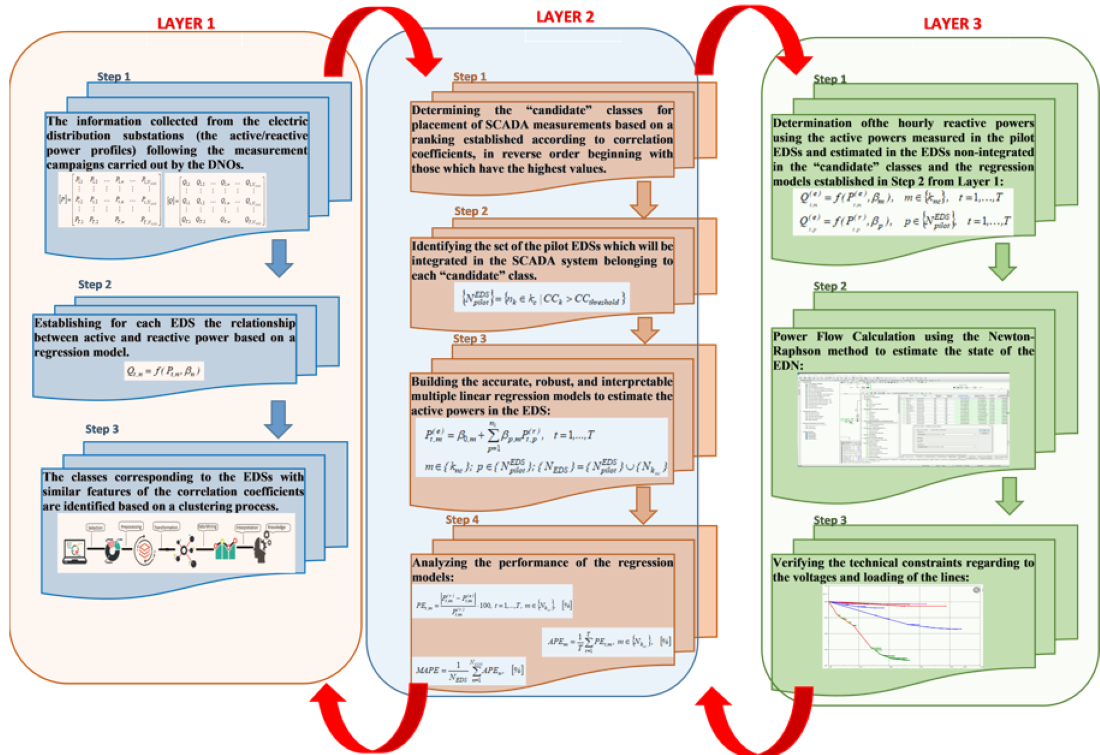
This section presents the information about the algorithms, methods and performance metrics included in the proposed three-layer iterative framework for the optimal placement of SCADA measurements with clustering-based EDS selection to estimate the state of the MV EDNs. Figure 3 illustrates the flow chart of the proposed framework.
The three-layer framework improves the solution by continuously updating the subsets of the decision variables. The details presented below regarding each layer include the developed mathematical tool.
2.1. Layer 1
Step 1. The information collected from the electric distribution substations (the active and reactive power profiles) following the measurement campaigns carried out by the DNOs represents input data. These profiles are recorded in the database and uploaded in the matrices [P] and [Q] having the sizes TxNEDS, where T represents the period used in the measurement campaigns to record the data with various sampling steps (usually 60 minutes) and NEDS correspond with the number of the EDSs from the analysed EDN.
Step 2. The correlation coefficients are calculated between each two EDSs (n and m, n ≠ m, n, m ∈ {NEDS}) from the analysed EDN and recorded in the matrix [CC], having the size (NEDSxNEDS).
where Cov(Pm, Pn) represents the covariance between the active power profiles from the set of the EDSs, generically noted n and m; σPn and σPm - the standard deviation of active powers associated with the EDSs m and n recorded in the time interval T.
Step 3. The classes corresponding to the EDSs with similar features of the correlation coefficients are identified based on a clustering process. The optimal partition in the classes will be determined using the K-Means clustering algorithm [20] and an internal test based on a performance indicator, namely the Silhouette Coefficient (SC) [21]. The clustering process includes the following phases:
- The NEDS vectors associated with the columns of the matrix [CC] should be integrated into K classes:
- 2.
- Determination the maximum number in which the NEDS electric distribution substations can be distributed using the relation [22]:
- 3.
- The vectors CCn, n = 1, …, NEDS, will be randomly assigned in the K classes of the EDSs.
- 4.
- The centroids Ck, k = 1, …, K and K = 2, …, Kmax, representing vectors with the size (NEDSx1) are calculated.
- 5.
- The repartition of the EDSs in in one of the K classes, K = 2, …, Kmax, will be based on the minimization of an objective function OF having the following expression:
- 6.
- The positions of the Ck centroids are re-adjusting through their recalculation using relation (7). In the case when all vectors CCn, n = 1, …, NEDS, are considered and re-labelled, Step 5 is repeated.
- 7.
- The silhouette coefficient for each partition K = 2, …, Kmax, will be calculated using the formula [23]:
- 8.
- The value of the silhouette coefficient SC(k) for each partition K = 2, …, Kmax is recorded in the vector [SC] and the maximum value is identified:
- 9.
- Determination of the optimal partition containing Kopt classes:
2.2. Layer 2
Step 1. Determining the “candidate” classes (notated with kc, kc ∈ {Kopt}) for placement of SCADA measurements based on a ranking established according to correlation coefficients, in reverse order beginning with those which have the highest values. The Decision Maker will impose a threshold (CCthreshold) for an average value of CC to choose the “candidate” classes [24].
Step 2. Identifying the set of the pilot EDSs which will be integrated in the SCADA system belonging to each “candidate” class.
where nk represents the number of the EDSs from each “candidate” class kc, , kc ∈ {Kopt}.
The pilot EDSs will represent the optimal places where be performed the SCADA measurements such that the load flow calculations to be carried out in the medium voltage distribution networks.
Step 3. Building the accurate, robust, and interpretable multiple linear regression models to estimate the active powers in the EDSs from the others classes that were not included in the set of the “candidate” classes. The models will use the pilot EDSs as regressors identified at Step 2.
where: {Nknc} – the set of the EDSs non-included in the “candidate” classes; {NpilotEDS} – the set of the pilot EDSs with SCADA measurements integrated; {NEDS} – the set of the EDSs from the analysed EDN; Pt,m(e) - the value of the active power estimated in the EDS "m" from the set {Nknc}, in [kW]; Pt,p(r) - the value of the active power measured in the pilot EDS “p” from the set {NpilotEDS}, in [kW]; β0,m – the constant coefficient of the linear regression model for each EDS from the set {Nknc}; βp,m – the coefficients corresponding with each regressor associated with the pilot EDS “p” from the set {NpilotEDS} in the linear regression model for each EDS from the set {Nknc}.
Step 4. Analyzing the performance of the regression models based on the following metrics: percentage error (PE), average percentage error (APE), and mean absolute percentage error (MAPE):
2.3. Layer 3
Step 1. Determination of the hourly reactive powers using the active powers measured in the pilot EDSs and estimated in the EDSs non-integrated in the “candidate” classes and the regression models established in Step 2 from Layer 1.
Step 2. Power Flow Calculation using the Newton-Raphson method to estimate the state of the EDN. The state variables recorded refer to the voltages on the MV side of the HV/MV EDS, the active and reactive power flows, the power/energy losses, and the active/reactive powers injected in the slack bus (the MV bus of the HV/MV EDS).
Step 3. Verifying the technical constraints regarding the voltages and loading of the lines. If there are violations of some limits, then the DNO can apply technical measures to bring the state values to the admissible limits provided in the performance standards or imposed by the manufacturers.
3. Results
A real urban MV EDN has been used to test the proposed framework. The END, supplied from an HV/MV (110/20 kV) EDS, contains three MV feeders with 39 MV/LV (20/0.4 kV) EDSs. Figure 4 presents the topology of the test MV EDN.
Table A1 from Appendix A includes each branch's length between two EDSs associated with each feeder. The EDN has the cross-section of the first branch (EDS – 1, EDS -14, and EDS – 29), with a size of 185 [mm2] (r0 = 0.157 [Ω/km] and x0 = 0.112 [Ω/km]), which is different from the other branches, equal to 150 [mm2] ((r0 = 0.194 [Ω/km] and x0 = 0.115 [Ω/km]). Also, the branch length is in the range [0.1 – 0.5] km, with a total length for the second feeder of 6.07 km higher than the other two feeders (3.36 km for the first feeder and 3.54 km for the third feeder, respectively). Figure 5 presents the synthesis of this information.
The rated power of the transformers, denoted with Sr, from the EDSs supplied by the three feeders is between 400 and 1000 kVA, see Table A2 from Appendix A. The total installed powers (calculated as the sum of the rated powers of the distribution transformers supplied by each feeder) are 7.15 MVA for the first feeder, 12.21 MVA for the second feeder, and 9.52 MVA for the third feeder, resulting in a total power of the EDN of 28.88 MVA, see Figure 6.
Step 1 of the first layer from the proposed methodology considers the building of a database with the active and reactive power profiles recorded in the matrix form, as seen in the relationships (1), based on a measurement campaign performed by the DNO during a week in the most loaded period.
Figure 7 and Figure 8 present the boxplots of the active and reactive powers associated with the measurement campaign.
A boxplot is a method that shows the locality, skewness, and spread groups of data through their respective quartiles. In addition to the box, there are also whiskers, which are lines that extend from the box to indicate variability outside the lower and upper limits of the range. These are referred to as box-and-whiskers and box-and-whiskers, respectively [25,26].
Table A3 and Table A4, from Appendix A, show the quartiles associated with the boxplot representation and two other statistical indicators (mean and standard deviation). The analysis of the information highlights that there are 14 EDSs with a high variation of the powers (9, 10, 12, 14, 17, 22, 27, 29, 30, 31, 33, 34, 38, and 39), 7 EDSs with slight variations (1, 2, 3, 4, 23, 24, and 25), and 18 EDSs with normal variations.
Step 2 of the first layer involves the calculation of the correlation coefficient between each of the two EDSs from the analysed EDN, which is recorded in the matrix [CC] and has a size [39x39]. Figure 9 presents the heatmap chart associated with matrix [CC] containing the values between -0.1 and 0.99. The vast majority of values are above 0.6. Still, there are also values close to 0 or even negative, which means that as one variable increases, the other decreases proportionally. Application of the K-means algorithm-based clustering process included in the last step of the first layer led to the classes corresponding to the EDSs with similar features of the correlation coefficients.
The maximum number of the clusters (named classes in the following) corresponded to a partition in 6 clusters. The internal test used the Silhouette Coefficient, and the algorithm identified the optimal number equal to 5 (for which the silhouette coefficient has the highest value, SC = 0.7168), see Figure 10. The representation of the silhouette coefficient for the optimal partition, Kopt = 5, is given in Figure 11.
Figure 12 highlights each class's percentage and the number of EDS it integrates. The analysis of the data indicates that the representative class is C5, containing 12 EDSs (30.77%), followed by classes C1 (10 EDSs, 25.64%), C2 (10 EDSs, 25.64%), C3 (5 EDSs, 12.82%), and C4 (2 EDSs, 5.13%).
The allocation of the EDSs in each class can be observed in Figure 13.
Two (Feeder 1 and Feeder 2) from three feeders have the EDSs associated with all classes, and one feeder (Feeder 3) contains the EDSs allocated to only three classes (C1, C2, and C5). Table 1 presents the statistical indicators corresponding to the quartiles (Q0 – Q4), mean (M), and standard deviation (SD) for the obtained classes following the clustering process.
The class with the values of the highest average correlation coefficient is C5, the range is [0.75, 0.82], and the smallest values are associated with C4 (0.4). The trend of the mean is the same, with the highest value recorded for class C5 (M = 0.79), followed by C1 (M = 0.74), C2 (M = 0.62), C3 (M = 0.62), and C4 (M = 0.4). The highest variation of the correlation coefficient belongs to class C2 (between 0.57 and 0.68), followed by C3 (between 0.59 and 0.64), C1 (between 0.71 and 0.75), and C5 (between 0.77 and 0.81), see Figure 14. The class C4 (having only 2 EDSs) was not taken into account, being unrepresentative for the analysis.
Step 1 of the second layer aims to set the threshold for CC at 0.75 to choose the candidate classes. This value is widely used in the literature for the minimum threshold value. The only class that meets this condition for the average correlation coefficient is C5. Thus, the EDSs from this class, identified with blue in Figure 13, will represent the optimal locations to integrate the SCADA system.
In the third step, the algorithm determines the multiple linear regression models to estimate the powers in the EDSs from the other classes not included in the set of the “candidate” classes. The models use as regressors the EDSs identified in the previous step.
Table 2 and Figure 15 present the APEs obtained based on the previously determined regression models for each EDS without integration into the SCADA system.
The APEs are equal to 0 for the EDSs from the candidate class (in our case, class C5), identified in bold in the table, because the system uploads the measurements from the SCADA system during the analysis period for these EDSs.
The results obtained with the proposed hybrid clustering-multiple linear regression (C-MLR) method have been compared with two other methods from the literature to demonstrate the performance of the proposed approach: the simple linear regression (SLR) method and the typical load profiles (TLPs) method. Estimating the powers from the EDSs based on the SLR method proposed in [15] contains the linear regression models between the reference, considered the MV bus of the supply HV/MV EDS, and the MV/LV EDSs from the EDN. Regarding the second method [19], each EDS has assigned a typical active and reactive profile depending on the energy consumption category obtained due to a clustering process.
The results indicate a substantial improvement in the estimation process of the APE values at the EDSs level with the proposed method compared to the SLR and TLPs methods. Table 4 and Figure 16, containing the statistical indicators associated with the quartiles Q0 – Q4, confirms this conclusion with a decrease of the maximum value from 30.9 % (calculated for SLR method) and 14.4% (calculated for TLPs method) to 6.3% and a median value (quartile Q2) from 11.8 % (calculated for SLR method) and 9.0 % (calculated for TLPs method) to 2.8 %. The SLR method led to the highest variation of the APEs in the range [4.1%, 30.9%], followed by the TLPs method with a range [3.1%, 25.4%]. The proposed method has the least variation, in the range [0.0%, 6.3%].
Regarding the MAPEs, Figure 17 presents the values of MAPEs calculated for the three methods. The value of MAPE decreases from 12.8% in the case of the SLR method to 9.9% in the case of the TLPs method and 2.6% (3 % approximately) in the case of the proposed C-MLR method (10% approximately).
In the following, Layer 3 of the methodology will use the results obtained with the proposed C-MLR method to estimate the state of the EDN associated with a day.
Because the voltages calculated at the level of the EDSs with the Newton-Raphson method based on the estimated powers are very close to the real data, being located between the allowable limits [+10%, -10%] compared with the nominal voltage, only the state variables obtained from the power flow calculations using the real and estimated active and reactive powers from the MV/LV EDSs associated with the injected active and reactive powers (Pinj and Qinj) from the slack bus (the 20 kV bus of the HV/MV EDS), the requested active and reactive powers (Preq and Qreq) at the level of the MV/LV EDSs from the EDN, the active and reactive power losses (ΔP and ΔQ), and capacitive reactive power of the cables (Qcap) are analysed. Table A5 and Table A6 from Appendix A present the hourly values obtained for these state variables. Table 4 contain the hourly percentage errors calculated for each state variable.
The data analysis highlights that higher errors than 1% are associated with 4 hours (3, 7, 8, and 18) for all state variables (less Qcap). However, the maximum value does not exceed 3% in the case of the active power loss at hour 7. Exceeding the 1% threshold is sporadically present, as other variables are, but they are tiny.
Table 5 and Figure 18 present the values corresponding to statistical indicators, which offer a clear image of the accuracy of the state estimation of the EDN. Each state variable has one or a maximum of two outliers, but the values cannot be considered as high as long as they are below a threshold accepted by the DNOs.
However, all state variables have MAPEs below 1%, as seen in Figure 19, which means an outstanding performance of the estimation process.
Finally, the proposed framework can offer the DNOs the state estimate synthesis based on the aggregated values quantified as energy amounts for the analysed period. Table 6 presents the values of the state variables obtained in both cases (real and estimated) and the errors.
The information presented in the table confirm again the accuracy of the estimation process where the state variables have the errors below 0.15%.
4. Conclusions and Discussions
A state estimation process analyses an electric network's operating conditions. It involves gathering all known information about the network to determine the most likely state. This process is commonly utilized in transmission networks to improve observability and optimize operating regimes. Although the estimation state process is frequently used in transmission networks, it has not been widely adopted in the distribution sector due to the lack of proper supervision and monitoring. Despite this, it can represent an essential EDN management component for DNOs.
In this context, determining the optimal number of EDSs integrated into a SCADA system to perform on-site measurements used in the state estimation process of the EDNs represents a challenge both from a technical and economic point of view for DNOs. It involves developing a robust framework incorporating algorithms to model the EDN's conditions accurately.
Thus, a three-layer framework for optimal placement of SCADA measurements with clustering-based EDS selection to estimate the state of the EDNs has been proposed. This framework has undergone rigorous testing to ensure its reliability and accuracy. The first layer includes the determination of the classes of the EDSs with similar features from the viewpoint of requested loads based on the K-means clustering algorithm. The second layer identifies the "candidate" classes and the pilot EDSs (representing the optimal solution) with the SCADA measurements placed. The optimal placement process aims to minimise the estimation errors based on the multiple linear regression models between the EDSs from the classes not included in the set of the "candidate" classes and the pilot EDSs. The third layer allows the state estimation of the EDNs based on the load values measured in the pilot EDEs (with the SCADA system implemented) and the other EDSs obtained through the regression models. The framework was tested in the case of a real urban EDN with 39 EDSs, where accuracy was ensured for on-site measurements in 12 of the 39 EDSs (representing 31% of EDSs integrated into the SCADA system). This solution is similar to the conclusions of the study from [3], where the integration degree in the SCADA system of the MV/LV EDSs at the level of most European DNOs is approximately 30%.
The power estimation process at the level of the EDSs for the analysed period indicated a decrease of MAPE from 12.8% in the case of the SLR method [15] to 9.9% in the case of the TLPs method [19] and 2.6% (3 % approximately) in the case of the proposed C-MLR method (10% approximately). This improvement in accuracy can significantly enhance the power estimation process, leading to more reliable network operations. Reading the state variables determined by a power flow calculation, the obtained MAPEs have been below 1%, which means an outstanding performance of the estimation process. Finally, the aggregated values quantified as energy amounts for the analysed period confirmed the accuracy of the estimation process, where the errors were below 0.15%.
The framework has been tested only in the EDNs without the distributed generation sources in this research stage. However, the authors are not stopping here. They are now working on an improved version that includes power injections from distributed generation sources. The degree of uncertainty at the level of the requested/injected powers is also being considered.
Author Contributions
Conceptualization, G.G. and V.D.; methodology, G.G. and V.D.; software, G.G.; validation, S.G.., M.-A.B., and V.D.; formal analysis, V.D., S.G., M.-A.B.; investigation, V.D., S.G. and M.-A.B.; resources, G.G.; data curation, G.G.; writing—original draft preparation, G.G.,V.D., S.G., and M.-A.B; writing—review and editing, G.G.; visualization, V.D.; supervision, G.G.; project administration, G.G.; funding acquisition, G.., S.G., M.-A.B., and V.D. All authors have read and agreed to the published version of the manuscript.
Funding
This research received no external funding.
Informed Consent Statement
Not applicable.
Data Availability Statement
The original contributions presented in the study are included in the article, further inquiries can be directed to the corresponding author.
Acknowledgments
In this section, you can acknowledge any support given which is not covered by the author contribution or funding sections. This may include administrative and technical support, or donations in kind (e.g., materials used for experiments).
Conflicts of Interest
The authors declare no conflicts of interest.
Abbreviations
The following abbreviations are used in this manuscript:
| EDN | electric distribution networks |
| DNO | distribution network operator |
| SCADA | supervisory, control, and acquisition system |
| EDS | electric distribution substations |
| MV | medium Voltage |
| HV | high Voltage |
| LV | low Voltage |
| RTU | remote terminal unit |
| MAPE | mean absolute percentage error |
| APE | average percentage error |
| PE | percentage error |
| SLR | simple linear regression |
| TLP | typical load profile |
| C-MLR | clustering-multiple linear regression |
Appendix A

Table A1.
The length of the branches associated with the three feeders.
| Branch |
Length [km] |
Feeder Allocated | Branch |
Length [mm2] |
Feeder Allocated | Branch |
Length [mm2] |
Feeder Allocated |
| EDS - 1 | 0.500 | Feeder 2 | 26 - 27 | 0.390 | Feeder 2 | 20 - 21 | 0.510 | Feeder 1 |
| 1 - 2 | 0.200 | Feeder 2 | 27 - 28 | 0.410 | Feeder 2 | 21 - 22 | 0.450 | Feeder 1 |
| 2 - 3 | 0.250 | Feeder 2 | 5 - 10 | 0.500 | Feeder 2 | EDS - 29 | 0.400 | Feeder 3 |
| 3 - 4 | 0.100 | Feeder 2 | 10 - 11 | 0.390 | Feeder 2 | 29 - 30 | 0.230 | Feeder 3 |
| 4 - 5 | 0.300 | Feeder 2 | 11 - 12 | 0.180 | Feeder 2 | 30 - 31 | 0.490 | Feeder 3 |
| 5 - 6 | 0.450 | Feeder 2 | 12 - 13 | 0.270 | Feeder 2 | 31 - 32 | 0.170 | Feeder 3 |
| 6 -7 | 0.280 | Feeder 2 | EDS - 14 | 0.600 | Feeder 1 | 32 - 33 | 0.340 | Feeder 3 |
| 7 - 8 | 0.310 | Feeder 2 | 14 - 15 | 0.180 | Feeder 1 | 33 - 34 | 0.480 | Feeder 3 |
| 8 - 9 | 0.210 | Feeder 2 | 15 - 16 | 0.290 | Feeder 1 | 34 - 35 | 0.210 | Feeder 3 |
| 2 - 23 | 0.350 | Feeder 2 | 16 - 17 | 0.350 | Feeder 1 | 35 - 36 | 0.350 | Feeder 3 |
| 23 - 24 | 0.260 | Feeder 2 | 17 - 18 | 0.230 | Feeder 1 | 36 - 37 | 0.370 | Feeder 3 |
| 24 - 25 | 0.400 | Feeder 2 | 18 - 19 | 0.400 | Feeder 1 | 37 - 38 | 0.210 | Feeder 3 |
| 25 - 26 | 0.320 | Feeder 2 | 19 - 20 | 0.350 | Feeder 1 | 38 - 39 | 0.290 | Feeder 3 |
Table A2.
The rated power of the transformers from the EDSs supplied by the three feeders.
| No. of EDS | Sr [kVA] | Feeder Allocated | No. of EDS | Sn [kVA] | Feeder Allocated | No. of EDS | Sn [kVA] | Feeder Allocated |
| 1 | 400 | Feeder 2 | 14 | 1000 | Feeder 1 | 27 | 630 | Feeder 2 |
| 2 | 400 | Feeder 2 | 15 | 1000 | Feeder 1 | 28 | 630 | Feeder 2 |
| 3 | 400 | Feeder 2 | 16 | 630 | Feeder 1 | 29 | 1000 | Feeder 3 |
| 4 | 400 | Feeder 2 | 17 | 1000 | Feeder 1 | 30 | 630 | Feeder 3 |
| 5 | 630 | Feeder 2 | 18 | 630 | Feeder 1 | 31 | 1000 | Feeder 3 |
| 6 | 630 | Feeder 2 | 19 | 630 | Feeder 1 | 32 | 630 | Feeder 3 |
| 7 | 630 | Feeder 2 | 20 | 630 | Feeder 1 | 33 | 1000 | Feeder 3 |
| 8 | 630 | Feeder 2 | 21 | 630 | Feeder 1 | 34 | 1000 | Feeder 3 |
| 9 | 1000 | Feeder 2 | 22 | 1000 | Feeder 1 | 35 | 1000 | Feeder 3 |
| 10 | 1000 | Feeder 2 | 23 | 400 | Feeder 2 | 36 | 630 | Feeder 3 |
| 11 | 630 | Feeder 2 | 24 | 400 | Feeder 2 | 37 | 630 | Feeder 3 |
| 12 | 1000 | Feeder 2 | 25 | 400 | Feeder 2 | 38 | 1000 | Feeder 3 |
| 13 | 1000 | Feeder 2 | 26 | 1000 | Feeder 2 | 39 | 1000 | Feeder 3 |
Table A3.
The statistical indicators (quartiles - Q0, Q1, Q2, Q3, Q4, mean – M, and standard deviation - SD) of the active powers from the EDSs, in [kW].
Table A3.
The statistical indicators (quartiles - Q0, Q1, Q2, Q3, Q4, mean – M, and standard deviation - SD) of the active powers from the EDSs, in [kW].
| No. EDS | Q0 | Q1 | Q2 | Q3 | Q4 | M | SD |
| 1 | 111.20 | 139.95 | 191.90 | 229.80 | 244.00 | 183.67 | 46.17 |
| 2 | 112.90 | 130.65 | 177.55 | 221.90 | 245.20 | 177.90 | 45.78 |
| 3 | 123.80 | 138.55 | 187.70 | 243.15 | 275.40 | 193.04 | 53.58 |
| 4 | 95.50 | 103.75 | 160.35 | 188.55 | 258.30 | 156.95 | 52.64 |
| 5 | 143.70 | 172.05 | 250.15 | 325.65 | 393.30 | 255.70 | 83.99 |
| 6 | 161.50 | 210.85 | 303.80 | 369.10 | 441.40 | 296.61 | 93.10 |
| 7 | 206.90 | 258.50 | 291.20 | 393.20 | 425.80 | 315.41 | 71.99 |
| 8 | 178.60 | 246.70 | 329.90 | 388.35 | 420.30 | 315.61 | 81.69 |
| 9 | 220.10 | 279.90 | 462.20 | 551.70 | 612.30 | 432.07 | 137.87 |
| 10 | 200.20 | 295.35 | 477.70 | 578.85 | 662.50 | 448.07 | 155.78 |
| 11 | 164.50 | 182.40 | 256.70 | 328.60 | 378.20 | 256.35 | 77.00 |
| 12 | 161.40 | 242.00 | 382.25 | 615.00 | 699.70 | 415.58 | 192.82 |
| 13 | 219.80 | 353.80 | 433.75 | 534.15 | 651.80 | 433.48 | 132.37 |
| 14 | 178.00 | 289.70 | 445.05 | 543.10 | 617.00 | 417.76 | 145.61 |
| 15 | 274.40 | 382.50 | 442.90 | 491.30 | 588.10 | 439.88 | 95.17 |
| 16 | 157.40 | 227.20 | 329.85 | 392.95 | 437.70 | 308.80 | 93.91 |
| 17 | 289.80 | 341.10 | 423.45 | 580.90 | 639.80 | 459.34 | 128.20 |
| 18 | 168.60 | 206.45 | 306.85 | 368.90 | 462.80 | 294.01 | 90.84 |
| 19 | 223.10 | 246.45 | 334.15 | 352.20 | 440.60 | 316.39 | 67.25 |
| 20 | 222.80 | 278.40 | 355.00 | 386.15 | 456.80 | 338.20 | 71.07 |
| 21 | 131.70 | 165.20 | 214.60 | 292.85 | 393.70 | 230.90 | 82.16 |
| 22 | 256.70 | 334.50 | 400.40 | 614.45 | 684.10 | 457.84 | 148.16 |
| 23 | 118.90 | 146.75 | 187.35 | 240.45 | 293.00 | 196.85 | 54.32 |
| 24 | 103.30 | 124.30 | 158.00 | 207.80 | 233.60 | 164.08 | 43.94 |
| 25 | 112.30 | 127.60 | 165.90 | 210.25 | 277.00 | 173.38 | 48.85 |
| 26 | 313.40 | 431.25 | 487.60 | 564.75 | 667.50 | 497.71 | 104.64 |
| 27 | 114.40 | 128.60 | 294.10 | 425.75 | 436.90 | 281.59 | 131.65 |
| 28 | 166.80 | 226.30 | 276.80 | 351.80 | 440.40 | 287.74 | 83.08 |
| 29 | 244.30 | 377.65 | 485.40 | 598.30 | 637.00 | 473.80 | 130.00 |
| 30 | 117.40 | 169.35 | 305.40 | 380.65 | 459.10 | 291.58 | 115.43 |
| 31 | 206.20 | 258.20 | 326.75 | 485.50 | 623.70 | 377.59 | 140.52 |
| 32 | 213.90 | 286.25 | 345.70 | 415.85 | 448.30 | 341.44 | 73.85 |
| 33 | 202.40 | 292.75 | 476.85 | 598.40 | 681.10 | 454.65 | 166.10 |
| 34 | 210.40 | 245.85 | 516.30 | 569.10 | 652.50 | 444.13 | 160.50 |
| 35 | 276.70 | 362.70 | 441.65 | 511.15 | 615.50 | 441.42 | 101.59 |
| 36 | 193.60 | 253.45 | 374.55 | 402.20 | 434.20 | 334.51 | 82.24 |
| 37 | 168.30 | 210.70 | 266.00 | 318.30 | 335.90 | 266.10 | 57.38 |
| 38 | 230.80 | 325.55 | 457.30 | 526.90 | 571.00 | 425.03 | 114.75 |
| 39 | 293.00 | 358.95 | 530.85 | 639.30 | 665.40 | 499.63 | 137.32 |
Table A4.
The statistical indicators (quartiles - Q0, Q1, Q2, Q3, Q4, mean – M, and standard deviation - SD) of the reactive powers from the EDSs, in [kVAr].
Table A4.
The statistical indicators (quartiles - Q0, Q1, Q2, Q3, Q4, mean – M, and standard deviation - SD) of the reactive powers from the EDSs, in [kVAr].
| No. EDS | Q0 | Q1 | Q2 | Q3 | Q4 | M | SD |
| 1 | 68.92 | 86.73 | 118.93 | 142.42 | 151.22 | 113.83 | 28.61 |
| 2 | 69.97 | 80.97 | 110.04 | 137.52 | 151.96 | 110.26 | 28.37 |
| 3 | 76.72 | 85.87 | 116.33 | 150.69 | 170.68 | 119.64 | 33.21 |
| 4 | 59.19 | 64.30 | 99.38 | 116.85 | 160.08 | 97.27 | 32.62 |
| 5 | 89.06 | 106.63 | 155.03 | 201.82 | 243.75 | 158.47 | 52.05 |
| 6 | 100.09 | 130.67 | 188.28 | 228.75 | 273.56 | 183.82 | 57.70 |
| 7 | 128.23 | 160.20 | 180.47 | 243.68 | 263.89 | 195.47 | 44.62 |
| 8 | 110.69 | 152.89 | 204.45 | 240.68 | 260.48 | 195.60 | 50.63 |
| 9 | 136.41 | 173.47 | 286.45 | 341.91 | 379.47 | 267.77 | 85.45 |
| 10 | 124.07 | 183.04 | 296.05 | 358.74 | 410.58 | 277.69 | 96.54 |
| 11 | 101.95 | 113.04 | 159.09 | 203.65 | 234.39 | 158.87 | 47.72 |
| 12 | 100.03 | 149.98 | 236.90 | 381.14 | 433.64 | 257.55 | 119.50 |
| 13 | 136.22 | 219.27 | 268.81 | 331.04 | 403.95 | 268.64 | 82.04 |
| 14 | 110.31 | 179.54 | 275.82 | 336.58 | 382.38 | 258.90 | 90.24 |
| 15 | 170.06 | 237.05 | 274.48 | 304.48 | 364.47 | 272.62 | 58.98 |
| 16 | 97.55 | 140.81 | 204.42 | 243.53 | 271.26 | 191.38 | 58.20 |
| 17 | 179.60 | 211.39 | 262.43 | 360.01 | 396.51 | 284.67 | 79.45 |
| 18 | 104.49 | 127.95 | 190.17 | 228.62 | 286.82 | 182.21 | 56.30 |
| 19 | 138.26 | 152.74 | 207.09 | 218.27 | 273.06 | 196.08 | 41.68 |
| 20 | 138.08 | 172.54 | 220.01 | 239.31 | 283.10 | 209.60 | 44.04 |
| 21 | 81.62 | 102.38 | 133.00 | 181.49 | 243.99 | 143.10 | 50.92 |
| 22 | 159.09 | 207.30 | 248.15 | 380.80 | 423.97 | 283.74 | 91.82 |
| 23 | 73.69 | 90.95 | 116.11 | 149.02 | 181.59 | 122.00 | 33.67 |
| 24 | 64.02 | 77.03 | 97.92 | 128.78 | 144.77 | 101.69 | 27.23 |
| 25 | 69.60 | 79.08 | 102.82 | 130.30 | 171.67 | 107.45 | 30.27 |
| 26 | 194.23 | 267.26 | 302.19 | 350.00 | 413.68 | 308.45 | 64.85 |
| 27 | 70.90 | 79.70 | 182.27 | 263.86 | 270.77 | 174.51 | 81.59 |
| 28 | 103.37 | 140.25 | 171.55 | 218.03 | 272.94 | 178.32 | 51.49 |
| 29 | 151.40 | 234.05 | 300.82 | 370.79 | 394.78 | 293.64 | 80.57 |
| 30 | 72.76 | 104.95 | 189.27 | 235.91 | 284.52 | 180.70 | 71.53 |
| 31 | 127.79 | 160.02 | 202.50 | 300.89 | 386.53 | 234.01 | 87.08 |
| 32 | 132.56 | 177.40 | 214.25 | 257.72 | 277.83 | 211.61 | 45.77 |
| 33 | 125.44 | 181.43 | 295.53 | 370.86 | 422.11 | 281.76 | 102.94 |
| 34 | 130.39 | 152.36 | 319.97 | 352.70 | 404.38 | 275.25 | 99.47 |
| 35 | 171.48 | 224.78 | 273.71 | 316.78 | 381.45 | 273.57 | 62.96 |
| 36 | 119.98 | 157.07 | 232.13 | 249.26 | 269.09 | 207.31 | 50.97 |
| 37 | 104.30 | 130.58 | 164.85 | 197.26 | 208.17 | 164.91 | 35.56 |
| 38 | 143.04 | 201.76 | 283.41 | 326.54 | 353.87 | 263.41 | 71.11 |
| 39 | 181.59 | 222.46 | 328.99 | 396.20 | 412.38 | 309.64 | 85.10 |
Table A5.
The state variables calculated based on the active and reactive power profiles estimated with the C-MLR method.
Table A5.
The state variables calculated based on the active and reactive power profiles estimated with the C-MLR method.
| Hour |
Pinj [MW] |
Qinj [MVAr] |
Preq [MW] |
Qreq [MVAr] |
ΔP [MW] |
ΔQ [MVAr] |
Qcap [MVAr] |
| 1 | 11.325 | 7.099 | 11.294 | 7.580 | 0.031 | 0.020 | 0.502 |
| 2 | 9.850 | 6.116 | 9.827 | 6.604 | 0.023 | 0.015 | 0.502 |
| 3 | 8.762 | 5.323 | 8.739 | 5.812 | 0.023 | 0.012 | 0.502 |
| 4 | 8.127 | 4.959 | 8.111 | 5.451 | 0.016 | 0.010 | 0.502 |
| 5 | 7.858 | 4.780 | 7.843 | 5.272 | 0.015 | 0.010 | 0.502 |
| 6 | 7.888 | 4.798 | 7.873 | 5.291 | 0.015 | 0.010 | 0.502 |
| 7 | 8.584 | 5.265 | 8.566 | 5.756 | 0.018 | 0.011 | 0.502 |
| 8 | 10.431 | 6.507 | 10.404 | 6.992 | 0.027 | 0.017 | 0.502 |
| 9 | 11.836 | 7.453 | 11.800 | 7.932 | 0.036 | 0.023 | 0.502 |
| 10 | 12.779 | 8.080 | 12.737 | 8.555 | 0.042 | 0.026 | 0.501 |
| 11 | 13.727 | 8.767 | 13.679 | 9.238 | 0.048 | 0.030 | 0.501 |
| 12 | 14.622 | 9.319 | 14.567 | 9.785 | 0.055 | 0.035 | 0.501 |
| 13 | 15.585 | 9.970 | 15.524 | 10.432 | 0.061 | 0.039 | 0.501 |
| 14 | 16.688 | 10.711 | 16.618 | 11.167 | 0.070 | 0.045 | 0.500 |
| 15 | 17.428 | 11.208 | 17.352 | 11.660 | 0.076 | 0.048 | 0.500 |
| 16 | 17.469 | 11.236 | 17.393 | 11.688 | 0.076 | 0.048 | 0.500 |
| 17 | 17.022 | 10.936 | 16.950 | 11.391 | 0.072 | 0.046 | 0.500 |
| 18 | 16.520 | 10.609 | 16.452 | 11.066 | 0.068 | 0.043 | 0.500 |
| 19 | 15.490 | 9.902 | 15.431 | 10.365 | 0.060 | 0.038 | 0.501 |
| 20 | 14.957 | 9.667 | 14.902 | 10.133 | 0.055 | 0.035 | 0.501 |
| 21 | 15.628 | 9.999 | 15.567 | 10.461 | 0.060 | 0.038 | 0.501 |
| 22 | 15.270 | 9.758 | 15.213 | 10.222 | 0.057 | 0.036 | 0.501 |
| 23 | 14.381 | 9.161 | 14.331 | 9.630 | 0.050 | 0.032 | 0.501 |
| 24 | 13.541 | 8.327 | 13.499 | 8.802 | 0.042 | 0.026 | 0.501 |
Table A6.
The state variables calculated based on the real active and reactive power profiles.
| Hour |
Pinj [MW] |
Qinj [MVAr] |
Preq [MW] |
Qreq [MVAr] |
ΔP [MW] |
ΔQ [MVAr] |
Qcap [MVAr] |
| 1 | 11.340 | 7.135 | 11.309 | 7.617 | 0.031 | 0.019 | 0.502 |
| 2 | 9.847 | 6.113 | 9.823 | 6.601 | 0.023 | 0.015 | 0.502 |
| 3 | 8.953 | 5.462 | 8.934 | 5.952 | 0.019 | 0.012 | 0.502 |
| 4 | 8.140 | 4.967 | 8.124 | 5.457 | 0.016 | 0.010 | 0.502 |
| 5 | 7.869 | 4.785 | 7.854 | 5.278 | 0.015 | 0.010 | 0.502 |
| 6 | 7.893 | 4.799 | 7.878 | 5.292 | 0.015 | 0.010 | 0.502 |
| 7 | 8.705 | 5.346 | 8.686 | 5.837 | 0.018 | 0.012 | 0.502 |
| 8 | 10.296 | 6.415 | 10.269 | 6.901 | 0.026 | 0.017 | 0.502 |
| 9 | 11.885 | 7.489 | 11.849 | 7.962 | 0.036 | 0.023 | 0.502 |
| 10 | 12.661 | 8.005 | 12.620 | 8.480 | 0.041 | 0.026 | 0.501 |
| 11 | 13.661 | 8.677 | 13.614 | 9.148 | 0.047 | 0.030 | 0.501 |
| 12 | 14.703 | 9.378 | 14.648 | 9.844 | 0.055 | 0.035 | 0.501 |
| 13 | 15.573 | 9.962 | 15.512 | 10.424 | 0.061 | 0.039 | 0.501 |
| 14 | 16.763 | 10.762 | 16.693 | 11.217 | 0.070 | 0.045 | 0.500 |
| 15 | 17.472 | 11.238 | 17.395 | 11.690 | 0.077 | 0.049 | 0.500 |
| 16 | 17.416 | 11.221 | 17.340 | 11.673 | 0.076 | 0.048 | 0.500 |
| 17 | 17.098 | 10.987 | 17.025 | 11.441 | 0.073 | 0.046 | 0.500 |
| 18 | 16.323 | 10.467 | 16.257 | 10.925 | 0.066 | 0.042 | 0.501 |
| 19 | 15.542 | 9.941 | 15.482 | 10.404 | 0.060 | 0.038 | 0.501 |
| 20 | 15.044 | 9.608 | 14.988 | 10.073 | 0.056 | 0.035 | 0.501 |
| 21 | 15.599 | 9.919 | 15.539 | 10.382 | 0.060 | 0.038 | 0.501 |
| 22 | 15.378 | 9.837 | 15.320 | 10.301 | 0.058 | 0.037 | 0.501 |
| 23 | 14.401 | 9.175 | 14.351 | 9.644 | 0.050 | 0.032 | 0.501 |
| 24 | 13.641 | 8.276 | 13.599 | 8.752 | 0.041 | 0.026 | 0.501 |
References
- Gnana Swathika, O.V.; Karthikeyan, A.; Karthikeyan, K.; Sanjeevikumar, P.; Sajju Karapparambil, T.; Babu, A. Critical review of SCADA And PLC in Smart Buildings and Energy Sector. Energy Reports, 2024, Volume 12, pp. 1518-1530. [CrossRef]
- Masri ,A; Al-Jabi, M. Toward fault tolerant modelling for SCADA based electricity distribution networks, machine learning approach. PeerJ Computer Science, 2021, Volume 7, e554. [CrossRef]
- European Commission, Distribution System Operators Observatory 2018. Overview of the electricity distribution system in Europe. 2019. Available online: https://ec.europa.eu/jrc/en/publication/eur-scientific-and-technical-research-reports/distribution-system-operators-observatory-2018 (accessed on 28 December 2024).
- Meletiou, A.; Vasiljevska, J.; Prettico, G.; Vitiello, S. Distribution System Operator Observatory 2022, Publication Office of the European Union, Luxembourg, 2023. Available online: https://publications.jrc.ec.europa.eu/repository/handle/JRC132379.
- Eyisi, C.; Lotfifard, S. Load Estimation for Electric Power Distribution Networks. In Proceedings of the 46th Power Sources Conference, Orlando, Florida, USA, 9-12 June 2014.
- Xie, C.; Jia, D.; Liu, J.; Sun, X.; Zhou, J.; Research on Operation Risk Prevention and Control Technology of Intelligent Distribution Network Based on Ultra Short Term Load Forecasting. In Proceedings of the 2020 IEEE 1st China International Youth Conference on Electrical Engineering, Wuhan, China, 1 – 4 November 2020.
- Benato, R.; Dambone Sessa, S.; Giannuzzi, G. M.; Pisani, C.; Poli, M.; Sanniti, F. A Novel Dynamic Load Modeling for Power Systems Restoration: An Experimental Validation on Active Distribution Networks. IEEE Access, 2022, Volume 10, pp. 89861-89875. [CrossRef]
- Chen, Y.; Fadda, M. G.; Benigni, A. Decentralized Load Estimation for Distribution Systems Using Artificial Neural Networks, IEEE Transactions on Instrumentation and Measurement, 2019, Volume 68, pp. 1333-1342. [CrossRef]
- Kong, X.; Zhang, X.; Zhang, X.; Wang, C.; Chiang, H. -D.; Li, P. Adaptive Dynamic State Estimation of Distribution Network Based on Interacting Multiple Model. IEEE Transactions on Sustainable Energy, 2022, Volume 13, pp. 643-652.
- Wang, R.; Qiu, H.; Gao, H.; Li, C.; Dong Z. Y.; Liu, J. Adaptive Horizontal Federated Learning-Based Demand Response Baseline Load Estimation, IEEE Transactions on Smart Grid, 2024, Volume 15, pp. 1659-1669. [CrossRef]
- Ebrahimi, M., Rastegar, M.; Arefi, M.M. Real-Time Estimation Frameworks for Feeder-Level Load Disaggregation and PEVs’ Charging Behavior Characteristics Extraction, IEEE Transactions on Industrial Informatics, 2022, Volume 18, pp. 4715-4724.
- Zhang, Y.; Wen, H.; Wu, Q.; Ai, Q. Optimal Adaptive Prediction Intervals for Electricity Load Forecasting in Distribution Systems via Reinforcement Learning, IEEE Transactions on Smart Grid, 2023, Volume 14, pp. 3259-3270. [CrossRef]
- Ali, M.; Adnan, M.; Tariq, M; Poor, H.V. Load Forecasting Through Estimated Parametrized Based Fuzzy Inference System in Smart Grids, IEEE Transactions on Fuzzy Systems, 2021, Volume 29, pp. 156-165. [CrossRef]
- Zhang, L.; Li, G.; Huang, Y.; Jiang, J.; Bie, Z.; Li, X. Distributed Baseline Load Estimation for Load Aggregators Based on Joint FCM Clustering, IEEE Transactions on Industry Applications, 2023, Volume 59, pp. 567-577.
- Grigoras, G.; Cartina, G. The Fuzzy Correlation Approach in Operation of Electrical Distribution Systems, The International Journal for Computation and Mathematics in Electrical and Electronic Engineering, 2013, Volume 32, pp. 1044-1066.
- Rong, H. Load Estimation of Complex Power Networks from Transformer Measurements and Forecasted Loads, Complexity, 2020, 2941809. Available online: https://www.hindawi.com/journals/ complexity/2020/2941809/ . [CrossRef]
- Chemetova, S.; Santos, P.; Ventim-Neves, M. Load Forecasting in Electrical Distribution Grid of Medium Voltage, Technological Innovation for Cyber-Physical Systems, 2016, Volume 470, pp. 340 – 349.
- Ding, N.; Benoit, C.; Foggia, G.; Bésanger, Y.; Wurtz, F. Neural Network-Based Model Design for Short-Term Load Forecast in Distribution Systems, IEEE Transactions on Power Systems, 2016, Volume 31, pp. 72 -81. [CrossRef]
- Grigoras, G.; Scarlatache, F.; Cartina, G. Load Estimation for Distribution Systems Using Clustering Techniques, In Proceedings of the 13th International Conference on Optimization of Electrical and Electronic Equipment, Brasov, Romania, 24 – 26 May 2012.
- Tahyudin, I.; Firmansyah, G.; Ivansyah, A. G.; Ma'arifah, W.; Lestari, L. Comparison of K-Means Algorithms and Fuzzy C-Means Algorithms for Clustering Customers Dataset, In Proceedings of the 1st International Conference on Smart Technology, Applied Informatics, and Engineering, Surakarta, Indonesia, 23 – 24 August 2022.
- Song, W.; Wang, Y.; Pan, Z.; A novel cell partition method by introducing Silhouette Coefficient for fast approximate nearest neighbor search, Information Sciences, 2023, Volume 642, 119216. [CrossRef]
- Grigoras, G.; Scarlatache, F. Processing of Smart Meters Data For Peak Load Estimation of Consumers, In Proceedings of the 9th International Symposium on Advanced Topics in Electrical Engineering, Bucharest, Romania, 9 – 7 May 2015.
- Shutaywi, M; Nezamoddin N. K. Silhouette Analysis for Performance Evaluation in Machine Learning with Applications to Clustering. Entropy, 2021, Volume 23, 759.
- Grigoras, G.; Dandea, V.; Neagu, B. -C.; Scarlatache, F. Load Estimation with the Clustering-Based Selection of the Electric Distribution Substations Integrated in SCADA System, In Proceedings of the 10th International Conference on Energy and Environment, Bucharest, Romania, 14 – 15 October 2021.
- Mirzargar, M.; Whitaker, R. T.; Kirby, R. M. Curve Boxplot: Generalization of Boxplot for Ensembles of Curve. IEEE Transactions on Visualization and Computer Graphics, 2014, Volume 20, pp. 2654-2663. [CrossRef]
- Kambale, W. V.; Deeb, A.; Bernabia, T.; Machot, F. A.; Kyamakya, K. A Boxplot Metadata Configuration Impact on Time Series Forecasting and Transfer Learning, In Proceedings of the 27th International Conference on Circuits, Systems, Communications and Computers (CSCC), Rhodes (Rodos) Island, Greece, 19 – 22 July 2023.
Figure 1.
The integration degree of the MV/LV EDSs in SCADA system.
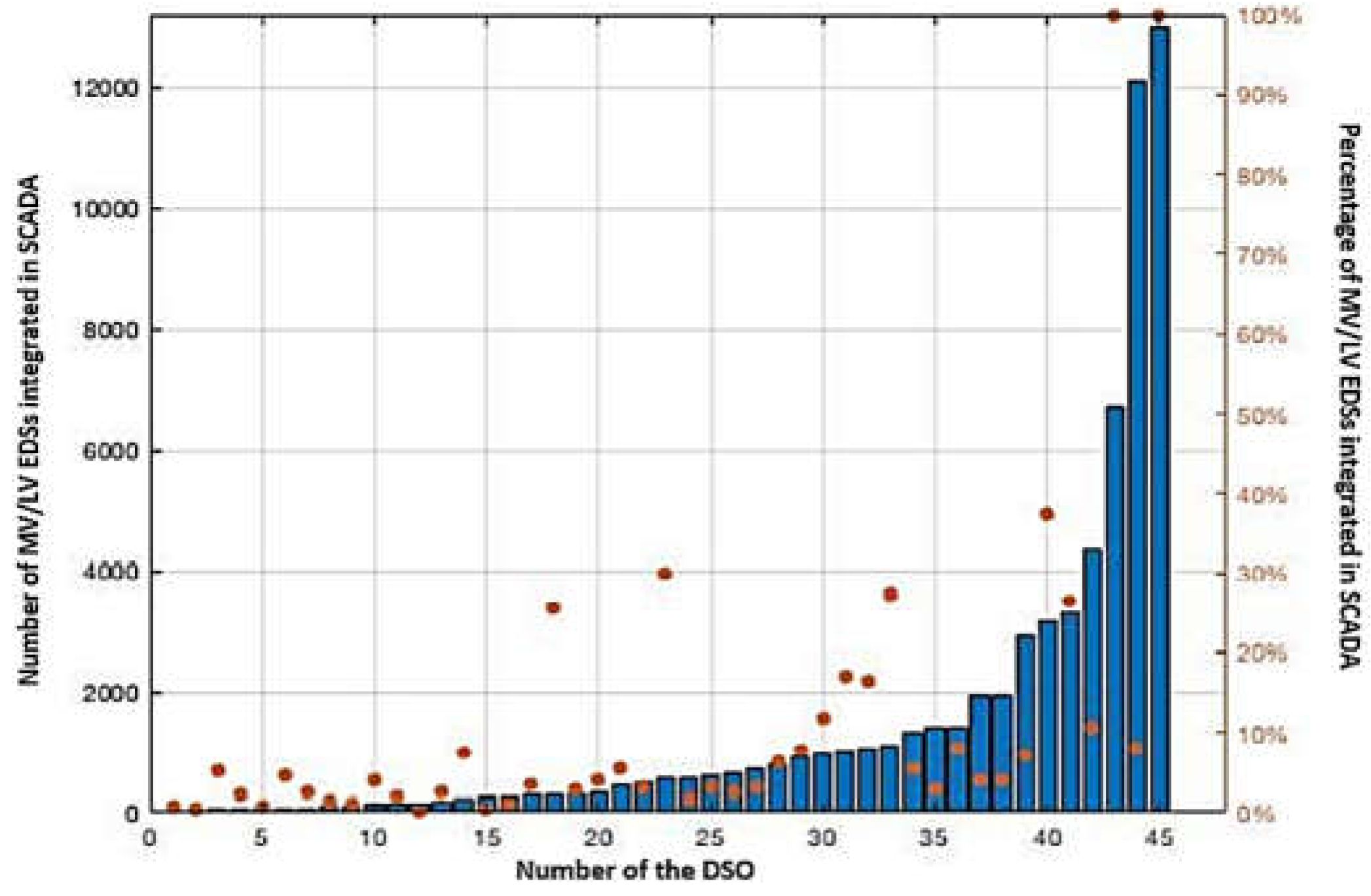
Figure 2.
The share of usual control types integrated into a SCADA system: (a) main control types, (b) – functions integrated inside each control type.
Figure 2.
The share of usual control types integrated into a SCADA system: (a) main control types, (b) – functions integrated inside each control type.
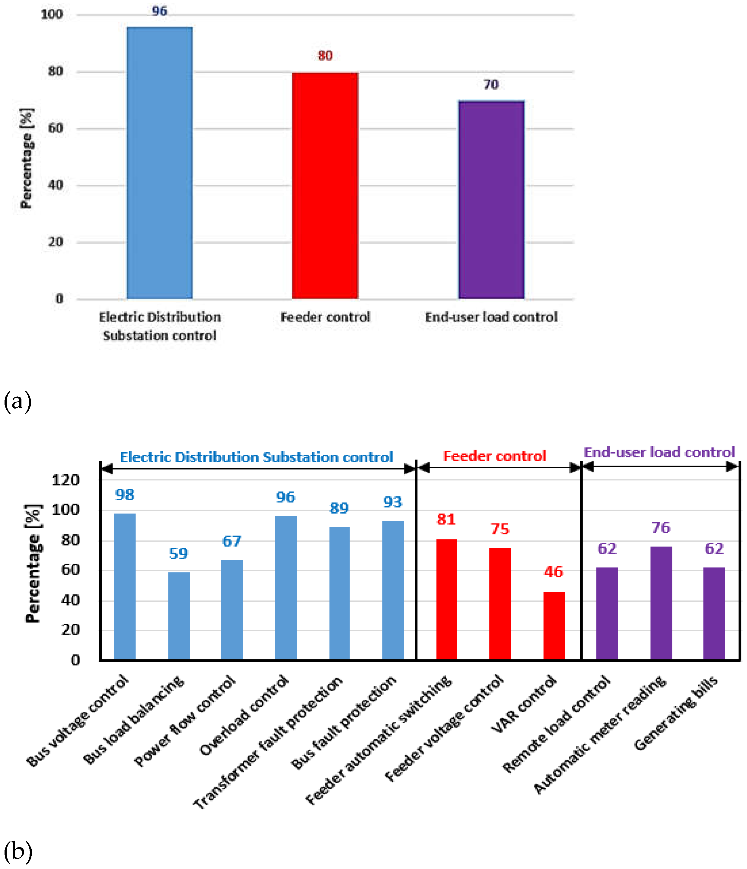
Figure 3.
The flow-chart of the proposed three-layer methodology.
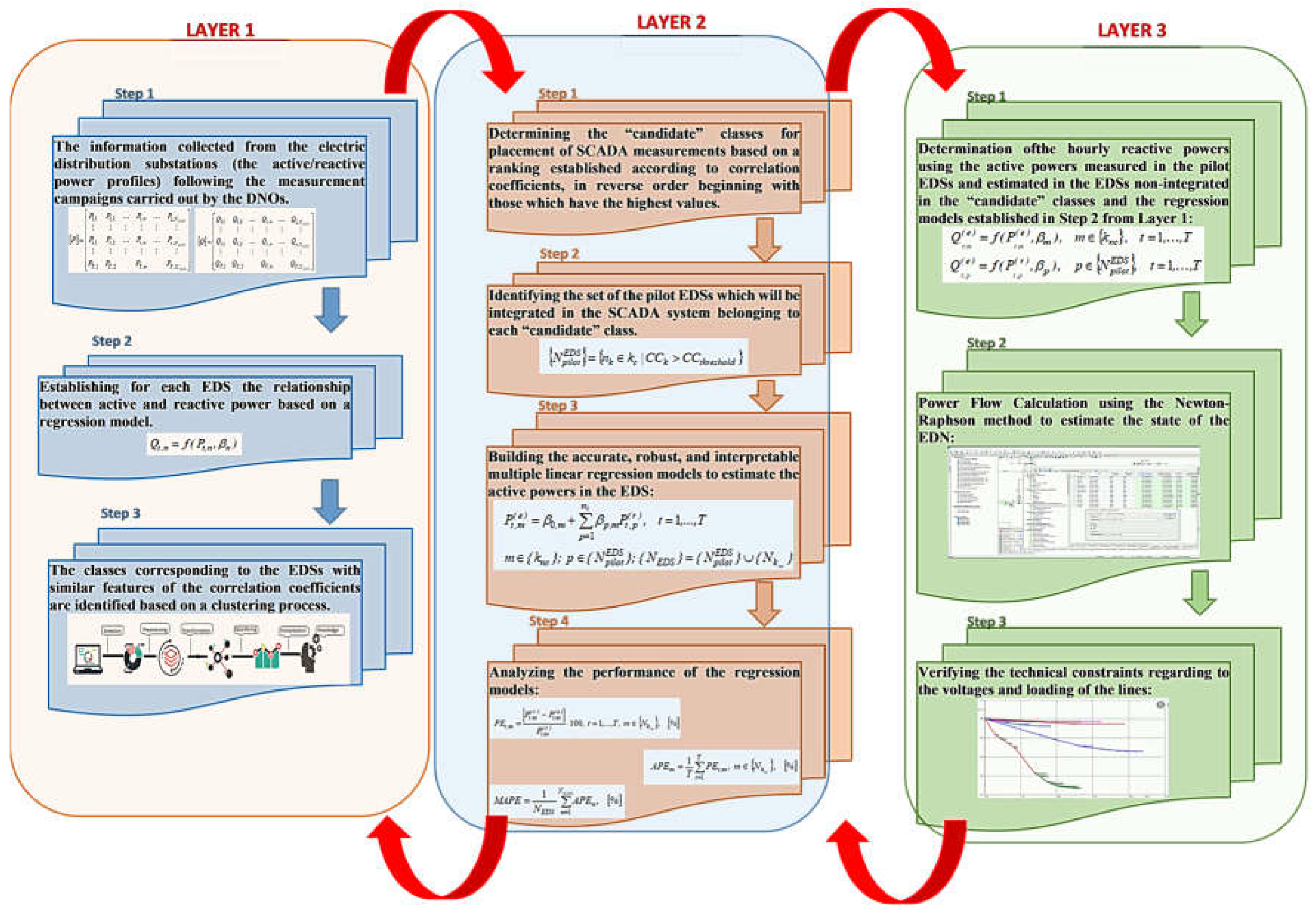
Figure 4.
The topology of the test 39-bus MV EDN.
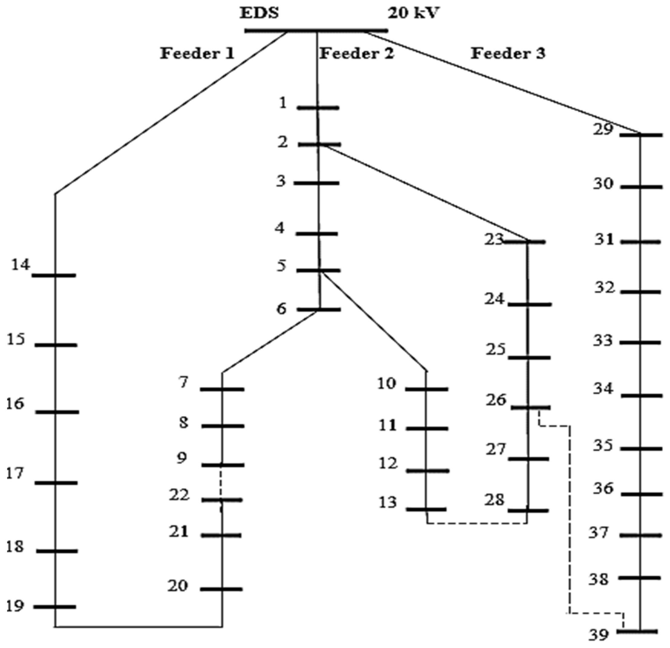
Figure 5.
The total length of each feeder from the test 39-bus MV EDN.
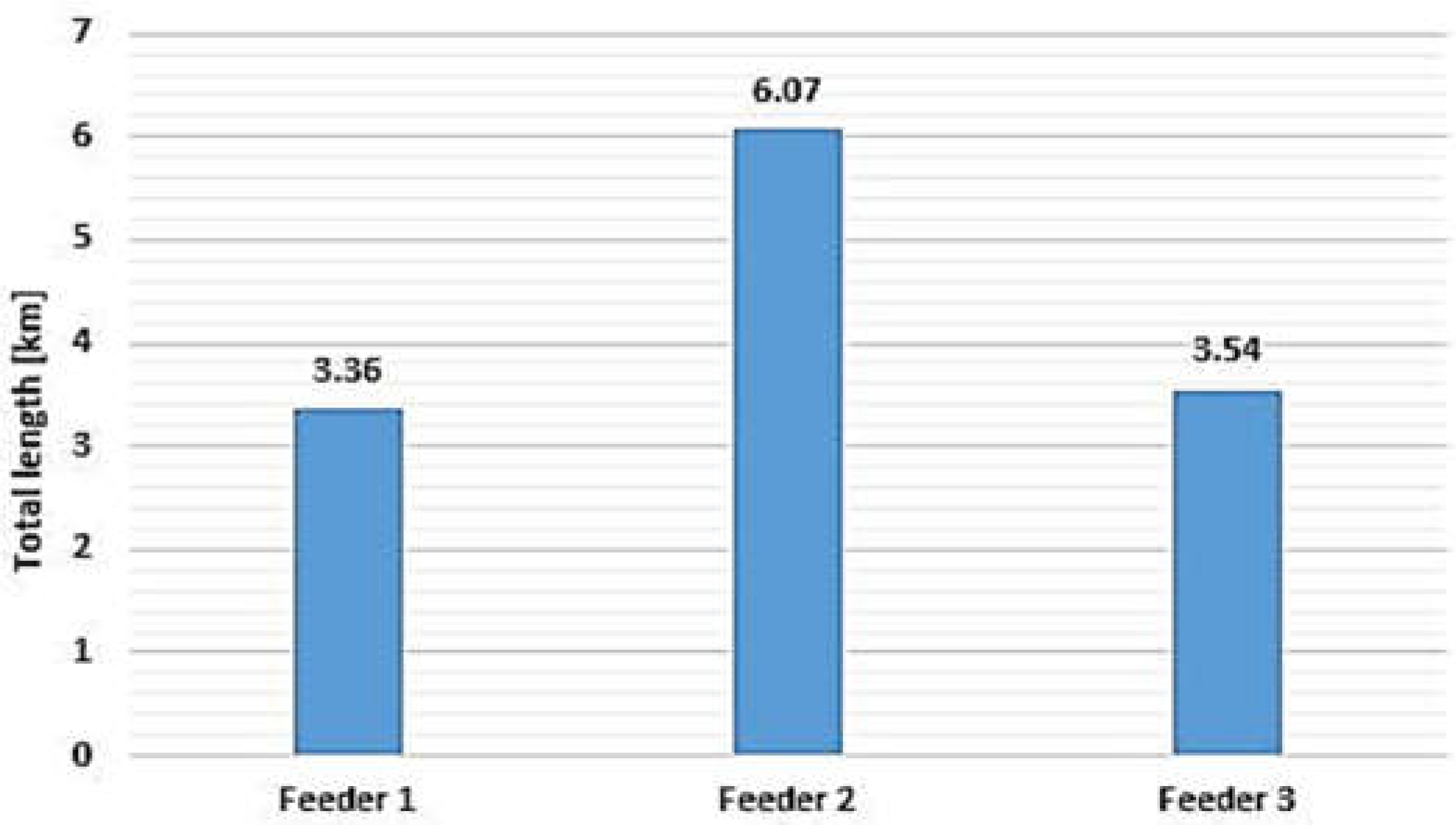
Figure 6.
The total installed power of each feeder from the test 39-bus MV EDN.
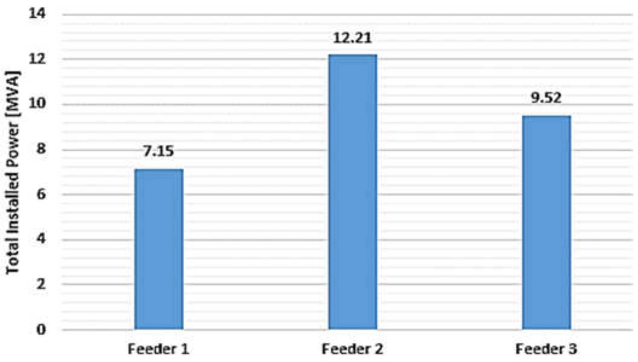
Figure 7.
The boxplots of the active powers from the EDSs.
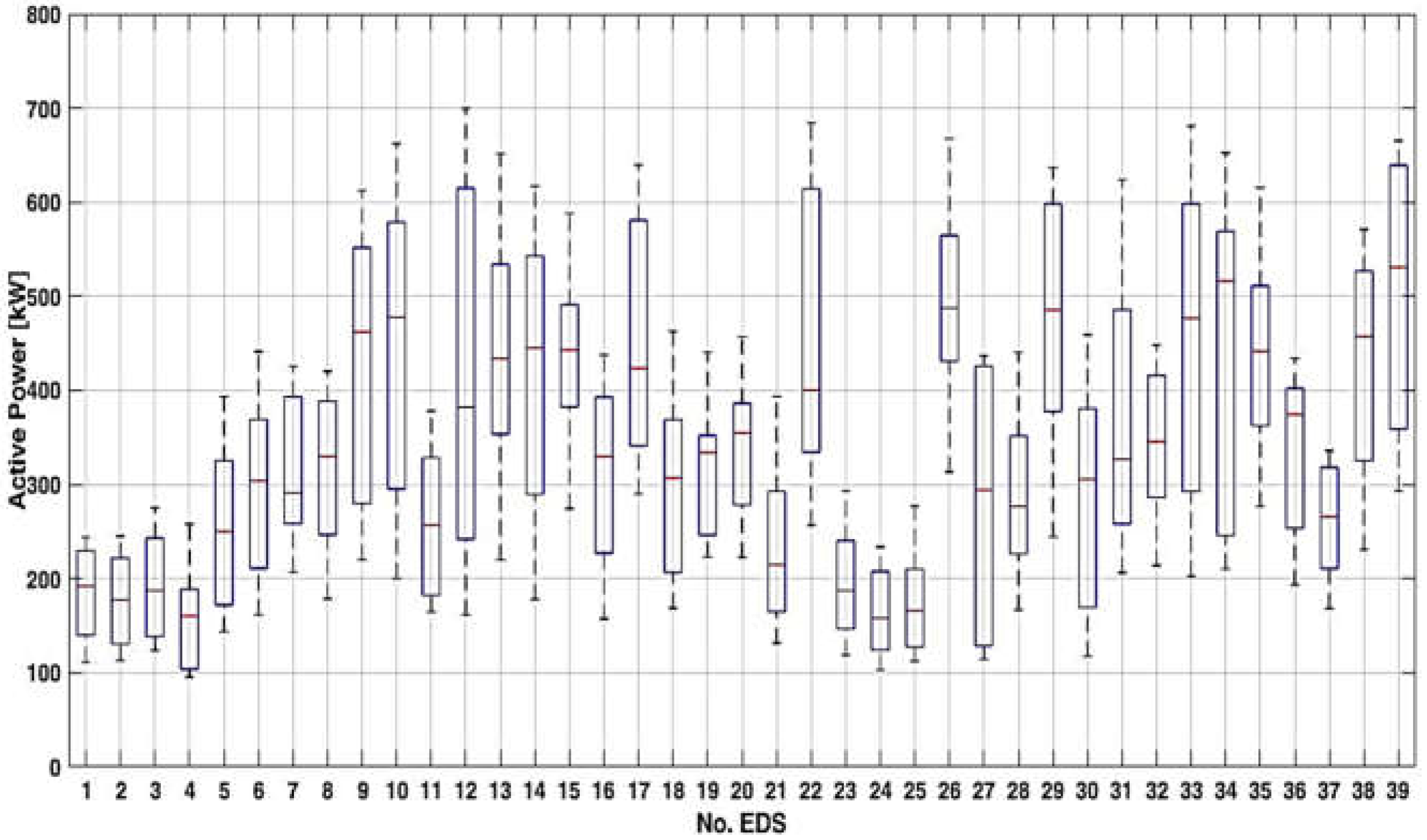
Figure 8.
The boxplots of the reactive powers from the EDSs.
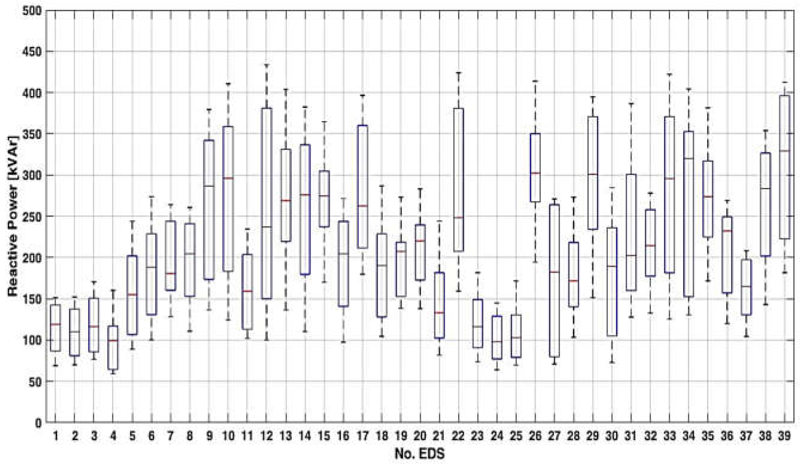
Figure 9.
The heatmap chart associated with correlation coefficients.
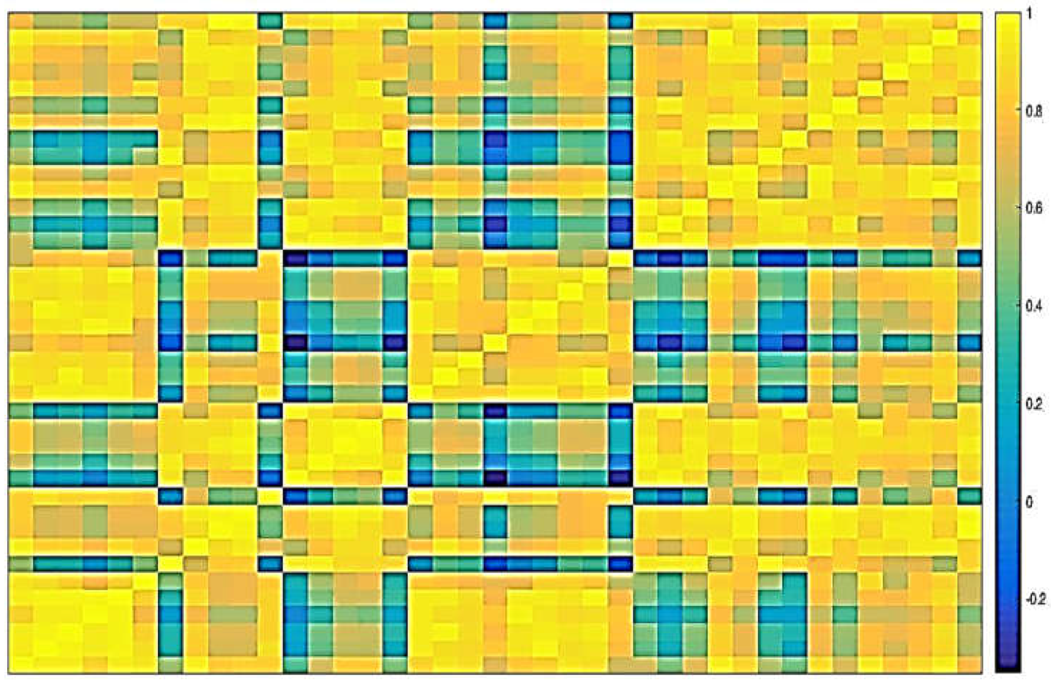
Figure 10.
The values of silhouette coefficient for the partitions K = 2 to Kmax = 6.
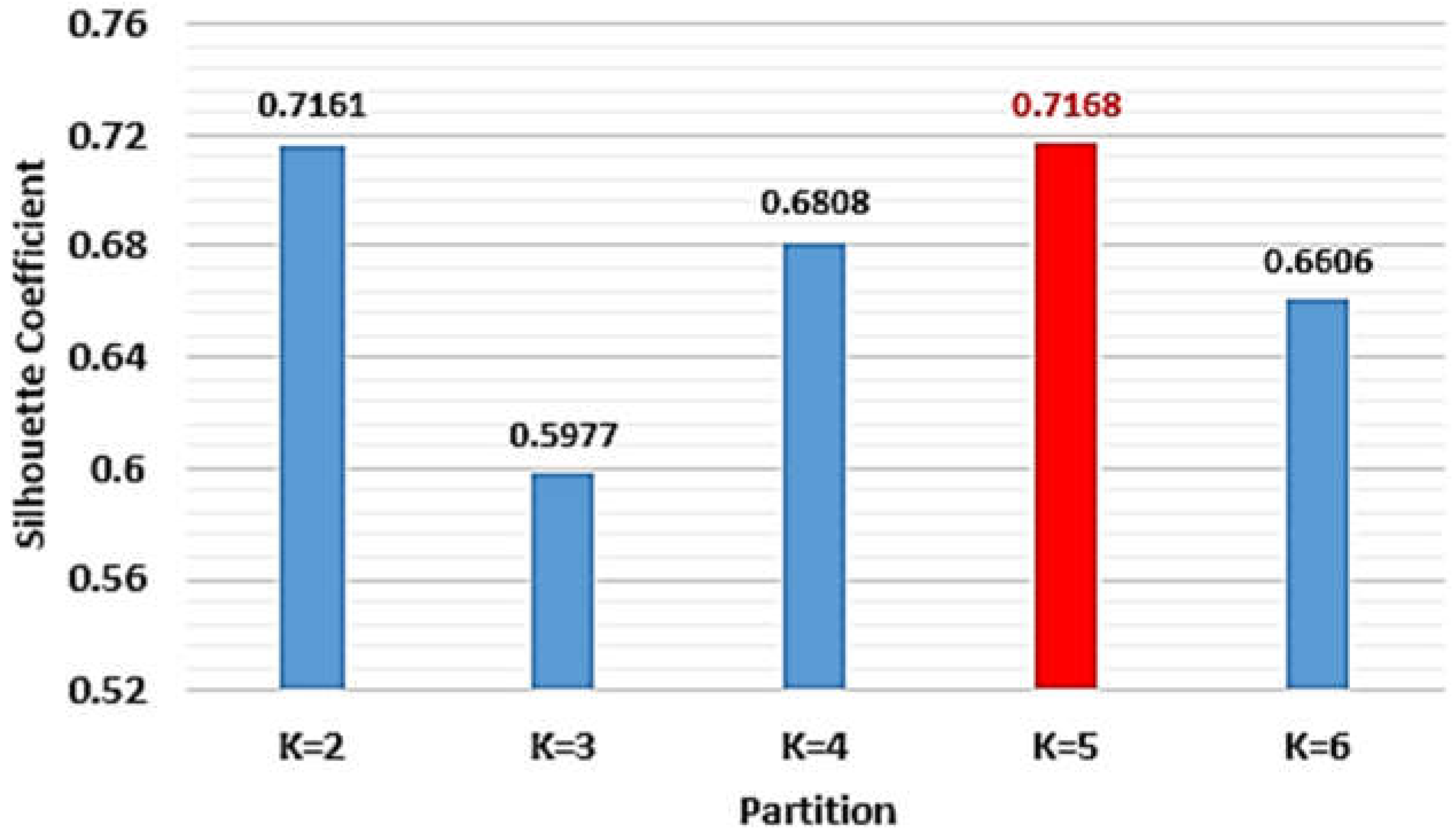
Figure 11.
The silhouette coefficient associated with the optimal partition, Kopt = 5.
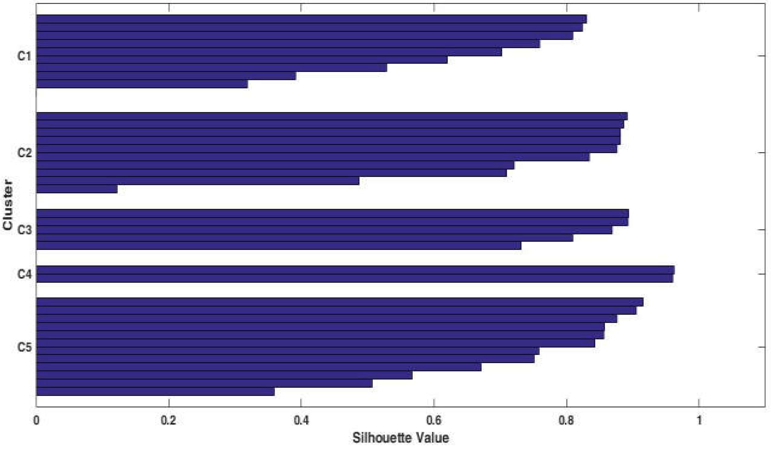
Figure 12.
The silhouette coefficient associated with the optimal partition, Kopt = 5.
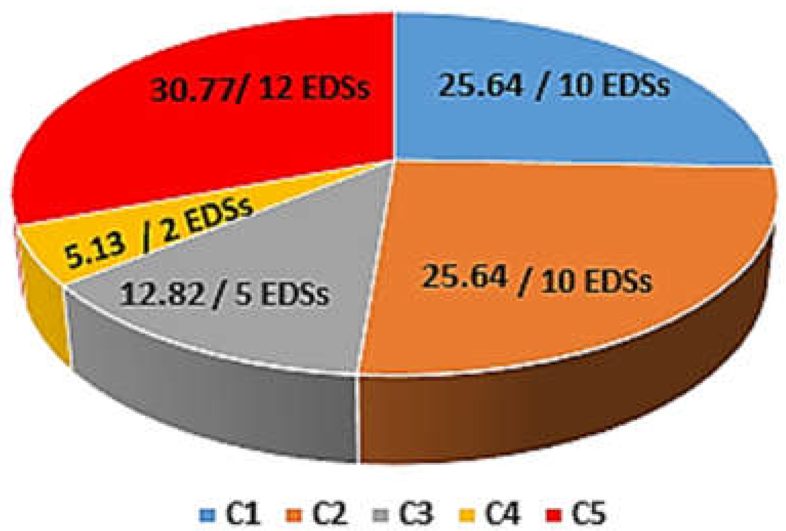
Figure 13.
The allocation of the EDSs to each class.
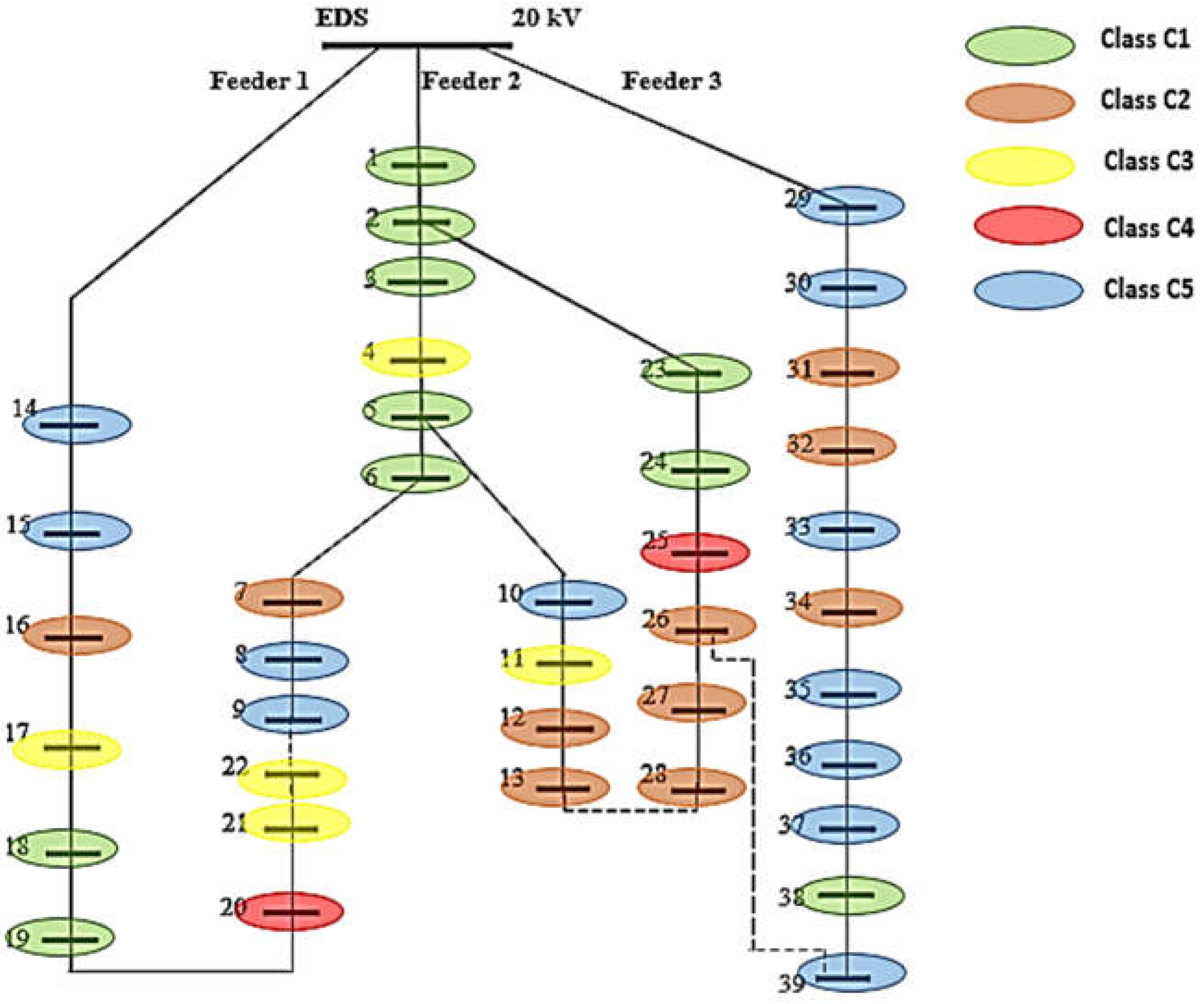
Figure 14.
The boxplot of the average correlations coefficients from the obtained classes.
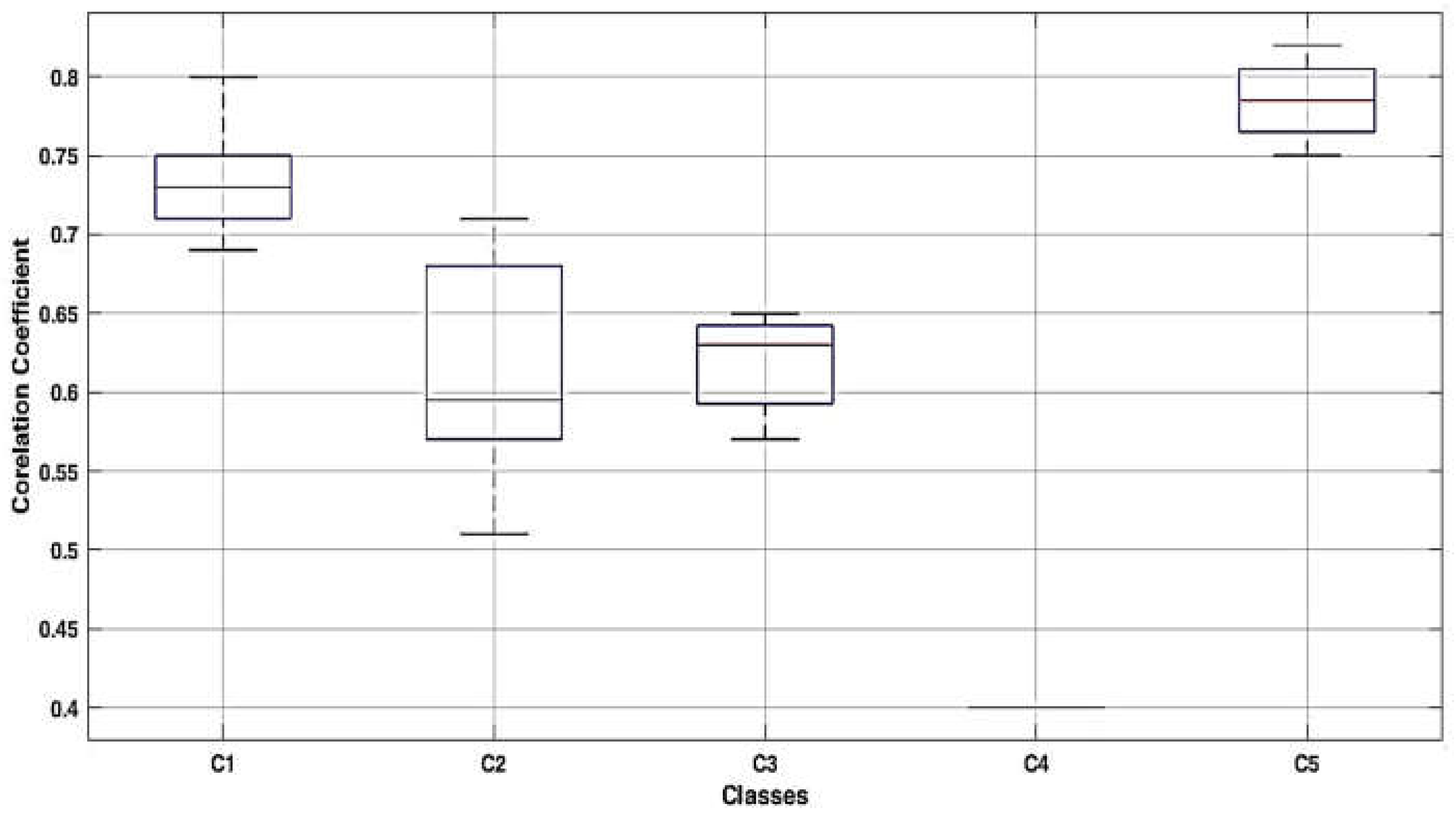
Figure 15.
The radar representation of APEs, in [%].
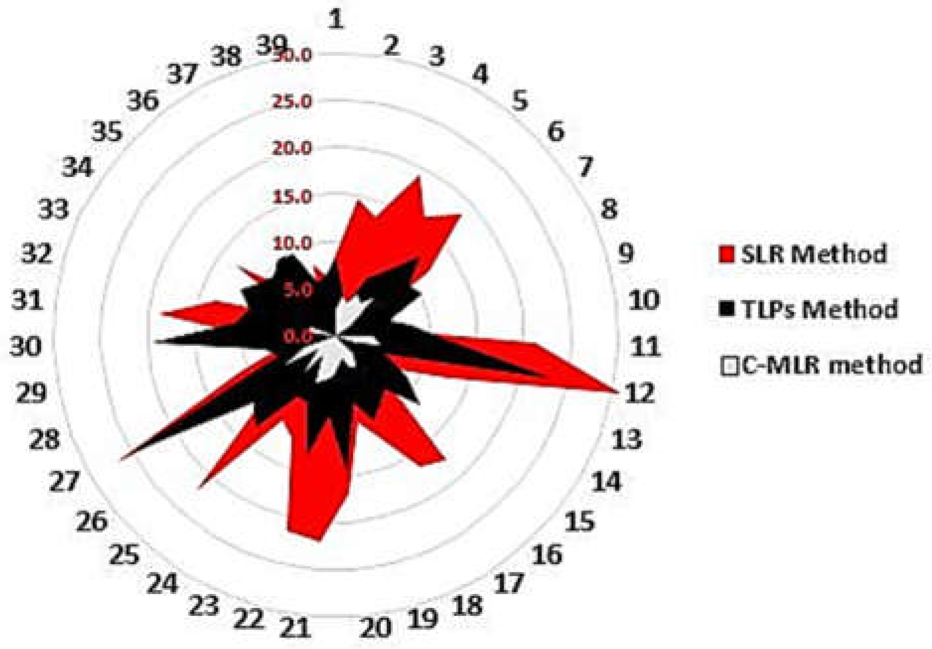
Figure 16.
The boxplot representation of the APEs, in [%].
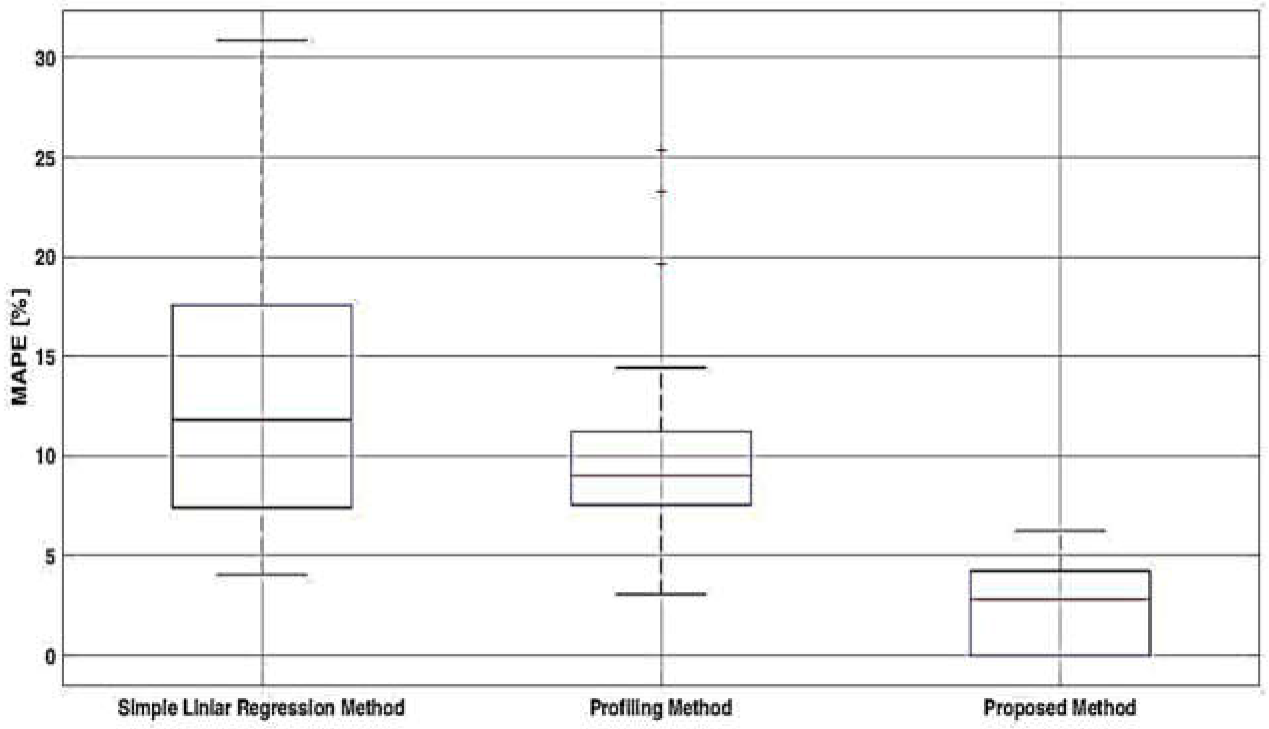
Figure 17.
The radar representation of MAPEs, in [%].
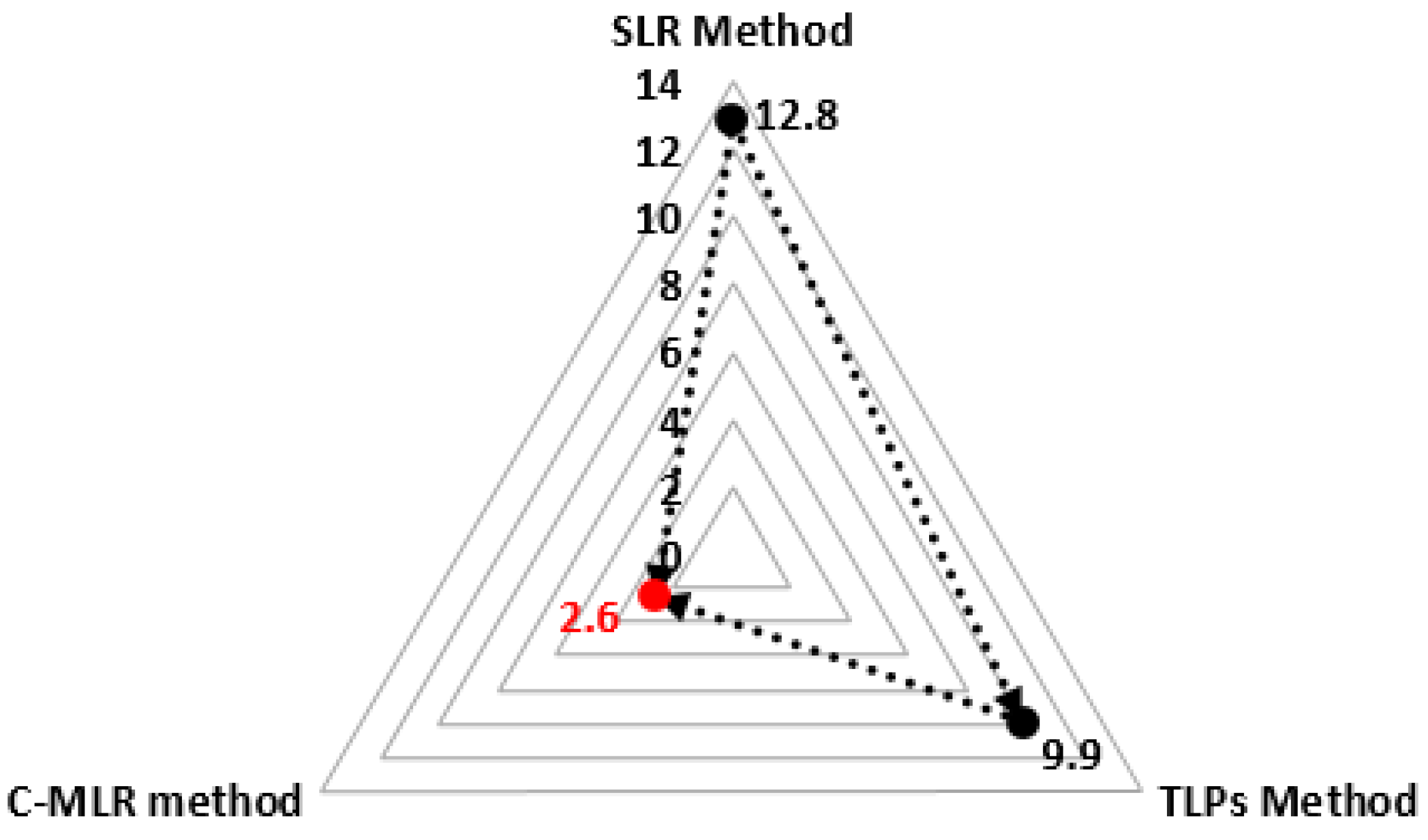
Figure 18.
The boxplot representation of the percentage errors calculated for the state variables.
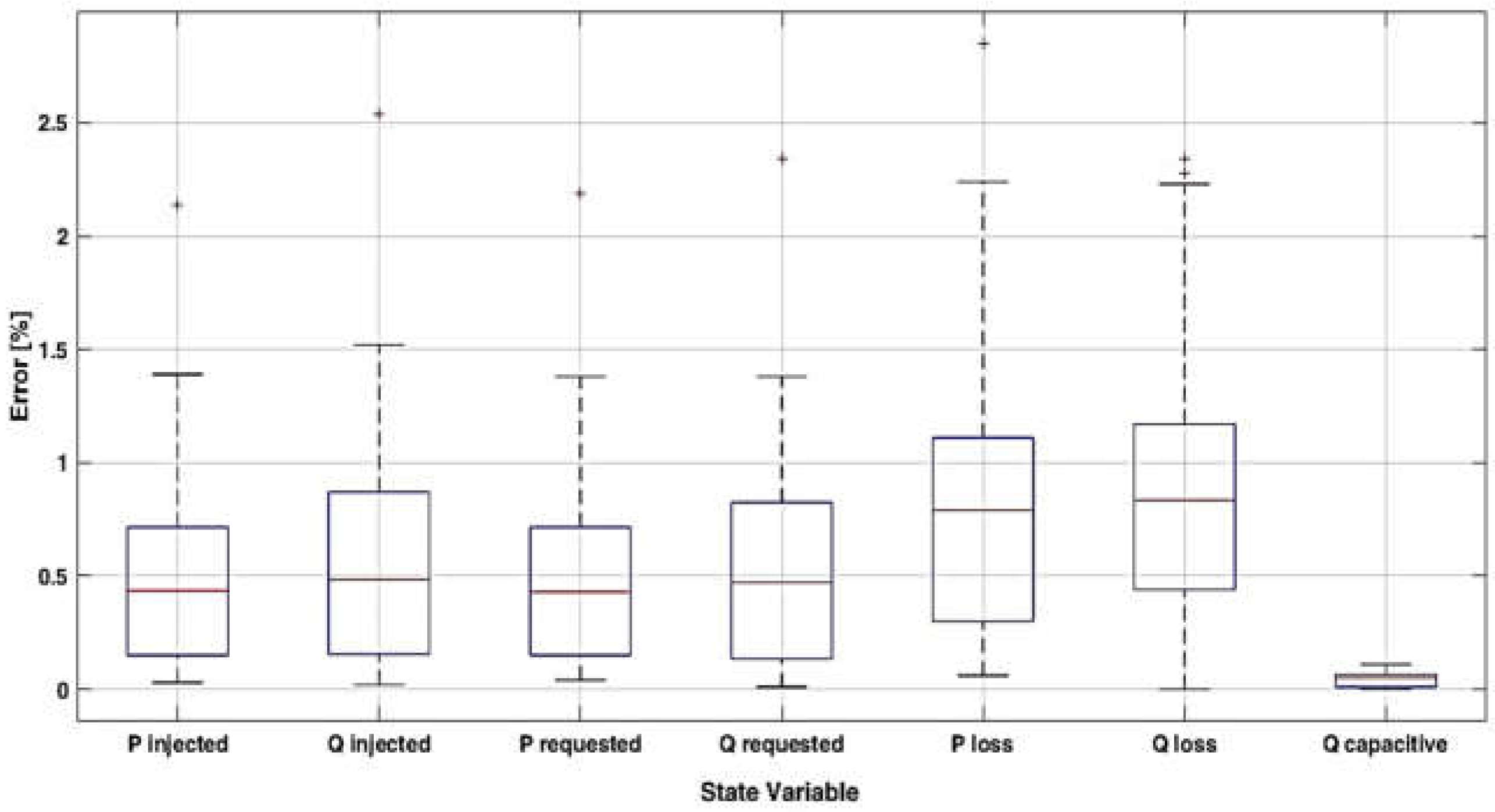
Figure 19.
MAPEs of the state variables.
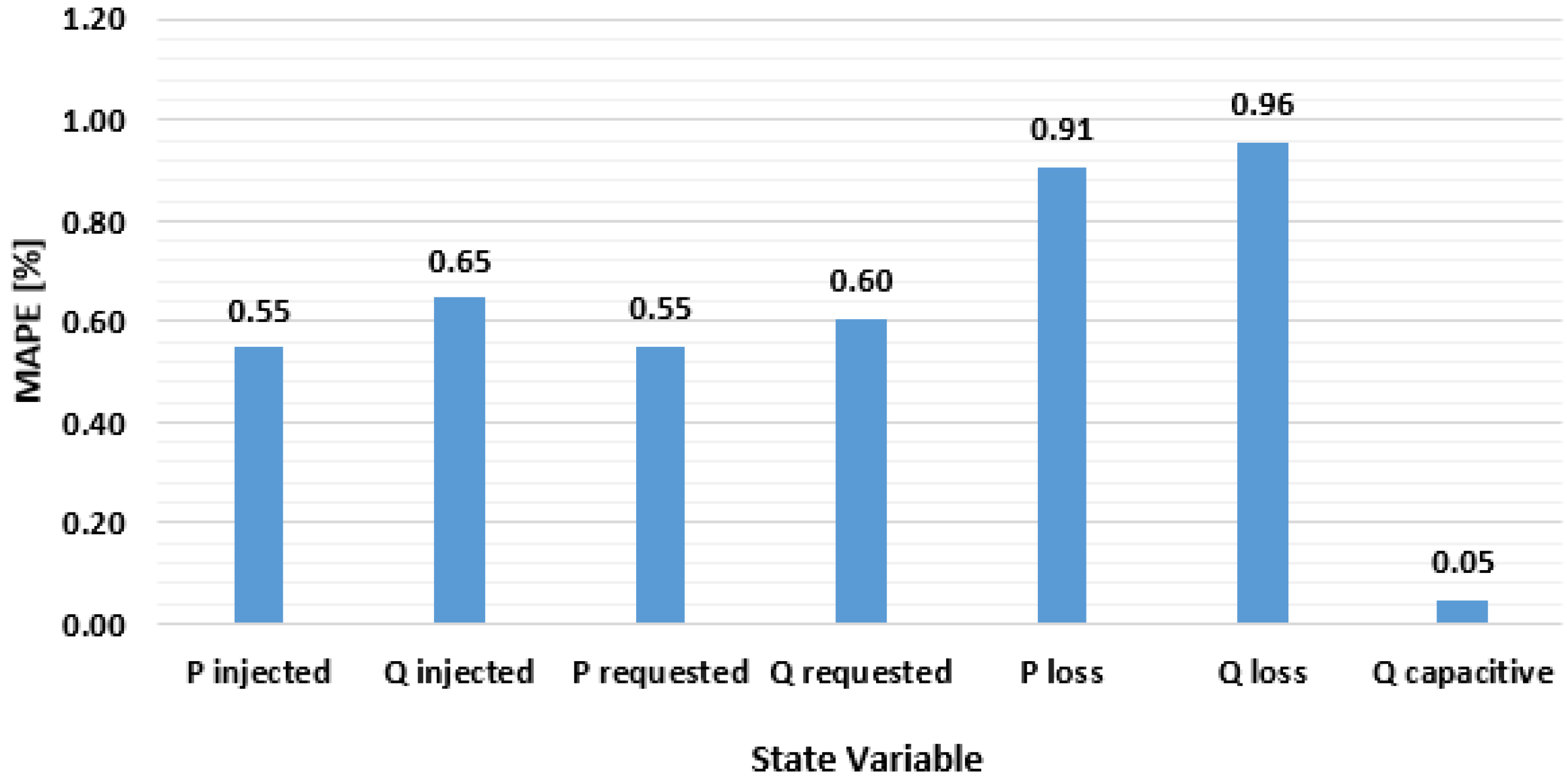
Table 1.
The statistical indicators associated with the obtained classes for the optimal partition.
| Class | Q0 | Q1 | Q2 | Q3 | Q4 | M | SD |
| C1 | 0.69 | 0.71 | 0.73 | 0.75 | 0.8 | 0.74 | 0.04 |
| C2 | 0.51 | 0.57 | 0.595 | 0.68 | 0.71 | 0.62 | 0.07 |
| C3 | 0.57 | 0.59 | 0.63 | 0.64 | 0.65 | 0.62 | 0.03 |
| C4 | 0.40 | 0.40 | 0.40 | 0.40 | 0.40 | 0.40 | 0 |
| C5 | 0.75 | 0.77 | 0.79 | 0.81 | 0.82 | 0.79 | 0.02 |
Table 2.
APEs calculated for the three methods, in [%].
| No. EDS | 1 | 2 | 3 | 4 | 5 | 6 | 7 | 8 | 9 | 10 | 11 | 12 | 13 | 14 | 15 | 16 | 17 | 18 | 19 | 20 |
| SLR Method | 8.6 | 14.7 | 13.3 | 19.4 | 15.8 | 18.5 | 12.0 | 4.2 | 6.4 | 5.2 | 21.2 | 30.9 | 12.8 | 7.3 | 5.8 | 17.8 | 16.6 | 11.8 | 9.6 | 16.9 |
| TLPs Method | 8.0 | 4.8 | 3.1 | 6.8 | 8.5 | 12.2 | 9.4 | 10.2 | 5.9 | 8.0 | 11.4 | 23.3 | 5.5 | 8.7 | 11.6 | 7.8 | 8.9 | 10.0 | 7.4 | 14.4 |
| C-MLR Method | 2.7 | 4.1 | 3.7 | 4.8 | 4.3 | 5.7 | 2.1 | 0.0 | 0.0 | 0.0 | 3.9 | 4.8 | 2.3 | 0.0 | 0.0 | 2.8 | 3.9 | 3.7 | 2.5 | 3.3 |
| No. EDS | 21 | 22 | 23 | 24 | 25 | 26 | 27 | 28 | 29 | 30 | 31 | 32 | 33 | 34 | 35 | 36 | 37 | 38 | 39 | |
| SLR Method | 22.0 | 21.5 | 11.8 | 10.8 | 22.3 | 8.4 | 27.0 | 10.8 | 5.7 | 8.3 | 19.0 | 13.2 | 4.6 | 12.9 | 6.8 | 8.1 | 4.1 | 7.8 | 6.2 | |
| TPLs Method | 8.6 | 13.2 | 7.8 | 7.5 | 13.0 | 11.2 | 25.4 | 6.4 | 7.7 | 19.6 | 10.6 | 9.6 | 11.2 | 9.7 | 9.0 | 10.0 | 9.6 | 6.0 | 6.5 | |
| C-MLR Method | 4.3 | 5.0 | 5.4 | 2.7 | 5.2 | 2.4 | 6.3 | 3.6 | 0.0 | 0.0 | 3.3 | 2.8 | 0.0 | 4.4 | 0.0 | 0.0 | 0.0 | 1.5 | 0.0 |
Table 3.
The statistical indicators associated with the APEs.
| Class | Q0 | Q1 | Q2 | Q3 | Q4 |
| SLR Method | 4.1 | 7.4 | 11.8 | 17.6 | 30.9 |
| TLPs Method | 3.1 | 7.6 | 9.0 | 11.2 | 25.4 |
| C-MLR Method | 0.0 | 0.00 | 2.8 | 4.2 | 6.3 |
Table 4.
The percentage errors calculated for the state variables, in [%].
| Hour | Pinj | Qinj | Preq | Qreq | ΔP | ΔQ | Qcap |
| 1 | 0.13 | 0.50 | 0.13 | 0.49 | 0.36 | 0.87 | 0.00 |
| 2 | 0.03 | 0.04 | 0.04 | 0.05 | 0.30 | 0.27 | 0.00 |
| 3 | 2.14 | 2.54 | 2.19 | 2.34 | 2.10 | 2.23 | 0.00 |
| 4 | 0.16 | 0.16 | 0.16 | 0.11 | 0.19 | 0.59 | 0.00 |
| 5 | 0.14 | 0.11 | 0.14 | 0.11 | 0.07 | 0.00 | 0.00 |
| 6 | 0.07 | 0.02 | 0.06 | 0.01 | 0.20 | 0.21 | 0.09 |
| 7 | 1.39 | 1.52 | 1.38 | 1.38 | 2.85 | 2.34 | 0.05 |
| 8 | 1.31 | 1.43 | 1.31 | 1.32 | 2.24 | 2.28 | 0.02 |
| 9 | 0.42 | 0.47 | 0.42 | 0.38 | 1.13 | 1.05 | 0.09 |
| 10 | 0.93 | 0.94 | 0.93 | 0.88 | 1.51 | 1.54 | 0.07 |
| 11 | 0.48 | 1.04 | 0.48 | 0.98 | 0.91 | 0.93 | 0.03 |
| 12 | 0.55 | 0.63 | 0.56 | 0.60 | 0.49 | 0.57 | 0.02 |
| 13 | 0.08 | 0.08 | 0.08 | 0.08 | 0.37 | 0.54 | 0.06 |
| 14 | 0.45 | 0.47 | 0.45 | 0.45 | 0.06 | 0.13 | 0.09 |
| 15 | 0.25 | 0.27 | 0.25 | 0.25 | 0.80 | 0.80 | 0.06 |
| 16 | 0.30 | 0.14 | 0.30 | 0.13 | 0.78 | 0.77 | 0.06 |
| 17 | 0.45 | 0.46 | 0.44 | 0.44 | 1.08 | 1.04 | 0.08 |
| 18 | 1.20 | 1.36 | 1.20 | 1.29 | 2.13 | 2.17 | 0.11 |
| 19 | 0.33 | 0.39 | 0.33 | 0.37 | 0.57 | 0.61 | 0.05 |
| 20 | 0.58 | 0.61 | 0.58 | 0.59 | 0.90 | 1.19 | 0.03 |
| 21 | 0.18 | 0.80 | 0.18 | 0.77 | 0.30 | 0.34 | 0.06 |
| 22 | 0.70 | 0.80 | 0.70 | 0.76 | 1.03 | 1.09 | 0.05 |
| 23 | 0.14 | 0.15 | 0.14 | 0.14 | 0.30 | 0.28 | 0.00 |
| 24 | 0.73 | 0.61 | 0.73 | 0.58 | 1.09 | 1.15 | 0.06 |
Table 5.
The statistical indicators of the percentage errors calculated for the state variables, in [%].
Table 5.
The statistical indicators of the percentage errors calculated for the state variables, in [%].
| State variable | Q0 | Q1 | Q2 | Q3 | Q4 |
| Injected active power | 0.03 | 0.15 | 0.44 | 0.72 | 2.14 |
| Injected reactive power | 0.02 | 0.16 | 0.49 | 0.87 | 2.54 |
| Requested active power | 0.04 | 0.15 | 0.43 | 0.72 | 2.19 |
| Requested active power | 0.01 | 0.14 | 0.47 | 0.83 | 2.34 |
| Active power loss | 0.06 | 0.30 | 0.79 | 1.11 | 2.85 |
| Reactive power loss | 0.00 | 0.44 | 0.84 | 1.17 | 2.34 |
| Capacitive reactive power | 0.00 | 0.01 | 0.05 | 0.07 | 0.11 |
Table 6.
The aggregated values of the state variables associated with the analysed period.
| Case |
WP inj [MWh] |
WQ inj [MVArh] |
WP req [MWh] |
WQ req [MVArh] |
ΔWP [MWh] |
ΔWQ [MVArh] |
WQcap [MVArh] |
| Real Data | 316.203 | 199.964 | 315.111 | 211.294 | 1.092 | 0.692 | 12.030 |
| Estimated Data | 315.766 | 199.950 | 314.670 | 211.286 | 1.096 | 0.693 | 12.028 |
| Error [%] | 0.138 | 0.007 | 0.140 | 0.004 | 0.330 | 0.032 | 0.014 |
Disclaimer/Publisher’s Note: The statements, opinions and data contained in all publications are solely those of the individual author(s) and contributor(s) and not of MDPI and/or the editor(s). MDPI and/or the editor(s) disclaim responsibility for any injury to people or property resulting from any ideas, methods, instructions or products referred to in the content. |
© 2025 by the authors. Licensee MDPI, Basel, Switzerland. This article is an open access article distributed under the terms and conditions of the Creative Commons Attribution (CC BY) license (http://creativecommons.org/licenses/by/4.0/).
Copyright: This open access article is published under a Creative Commons CC BY 4.0 license, which permit the free download, distribution, and reuse, provided that the author and preprint are cited in any reuse.


