
Submitted:
22 April 2025
Posted:
23 April 2025
You are already at the latest version
Abstract
This study aims to assess the power capacity of electrical conductors under the long-term expansion of distribution systems over a 10-year horizon, considering voltage quality constraints and reliability indicators. The MATPOWER library in Matlab was employed, along with the IEEE 15-bus and 33-bus distribution system test cases. A 5% annual load growth was simulated for each system, analyzing key parameters such as power losses, voltage deviation, and average failure rate. An algorithm was developed to perform a multi-criteria analysis, providing optimal solutions for system behavior in response to increasing demand. Given the close relationship between distribution systems and load growth, voltage quality and reliability indicators were evaluated annually to identify improvement opportunities, taking into account economic factors, implementation timelines, replacement of electrical components, and medium- and long-term investments. The proposed algorithm recommended upgrades to electrical conductors without significantly affecting system costs. For the initial year of the IEEE 15-bus system, enhancements were suggested for lines L1–L2, L2–L3, L3–L4, L2–L6, L3–L11, and L11–L12, allowing the system to operate without further modifications for five years, maintaining minimum voltages above 0.95 p.u. and reducing the average failure rate while demand continued to grow.
Keywords:
voltage profile
; power losses
; voltage quality
; reliability analysis
; average failure rate
1. Introduction
The electrical distribution system is responsible for delivering electric power to end users. Before reaching this stage, electricity undergoes generation and transmission processes, making distribution the final step in the power supply chain [1].
Key characteristics of distribution systems include the operating voltage level—typically in the range of 6 kV to 36 kV—used in both urban and rural areas [2], and distribution transformers, which reduce the voltage level to supply electricity safely and efficiently to end users [3].
As the final link in the power supply chain, the distribution system must ensure the reliable, secure, and efficient delivery of energy, maintaining proper power quality in terms of voltage and frequency [3,4].
Over time, distribution systems must dynamically adapt to increasing demand, considering parameters such as reliability, stability, and quality [5].
Power quality in a distribution system refers to its ability to deliver electricity in conditions suitable for use, without disturbances that may negatively affect end users [5,6]. Key parameters used to evaluate power quality include voltage (above 0.95 p.u.), frequency (around 60 Hz), flicker (rapid voltage variations), and interruptions (momentary outages).
Reliability refers to the system’s ability to supply electricity without interruptions or failures for as much time as possible, ensuring constant power availability for users [7]. The most commonly used reliability indicators are: interruption frequency, average failure rate, duration of interruptions, and restoration time [8].
Several factors affect power quality and reliability in distribution systems, including: external weather conditions (e.g., thunderstorms, landslides, strong winds), poor maintenance (e.g., lack of upkeep for transformers, cables, or substations), overloads (operation beyond capacity), technical or human failures (e.g., operational errors or equipment failures), and outdated infrastructure (e.g., aging systems not designed for growing demand) [9,10].
With technological advancement, electrical engineering continues to offer solutions to emerging power quality and reliability issues. These include: protection coordination [10], voltage control through sensor integration [11], and proposals for distributed generation near the distribution network [12].
Likewise, the implementation of systems with neural analysis (intelligent learning) has become increasingly relevant [9], as they can provide solutions based on the data they gather over time. Nevertheless, it is crucial to consider the current condition of distribution systems, especially since investment analysis focused on such systems is often neglected. These investments are essential for system development and growth and include key aspects such as new technologies, communication, sustainability, and resilience [12,13].
Although several methods exist to address problems related to increasing demand—considering both economic and sustainability aspects—there is a growing need for fast and efficient methods, particularly those based on single- or multi-criteria decision-making functions [14], which are both robust and accurate.
Multi-criteria decision analysis (MCDA) enables the incorporation of multiple criteria to deliver optimal solutions, while applying restrictions or initial conditions to the function [15]. Key features of MCDA include: evaluation capabilities (allowing the analysis of several variables—decisions should not rely on a single factor), qualitative or quantitative criteria, trade-offs (balancing between conflicting criteria), and weight assignment (based on each criterion’s relative importance) [19].
Decision-making within MCDA depends on the problem context, the identification of criteria, weight assignment, number of alternatives, and the application domain. Commonly used methods include: Analytic Hierarchy Process (AHP)—which uses pairwise comparisons among criteria and alternatives; Linear Weighting—where weights are multiplied by values for each alternative; and Technique for Order of Preference by Similarity to Ideal Solution (TOPSIS)—which selects the alternative closest to the ideal solution and farthest from the worst-case scenario. These techniques help balance and prioritize conflicting criteria [17,18].
When properly applied, with well-defined criteria and parameter values, MCDA can be used to analyze the performance of a distribution system under increasing demand. This allows the optimization of power quality, reliability, and economic performance, producing effective results in a reduced amount of time.
2. Methodology
2.1. Impact of Demand Growth
The increase in demand within electrical distribution systems generates significant challenges, such as increased load on existing infrastructure, the risk of overloading, higher technical losses, and the deterioration of service quality and reliability delivered to end users. In order to mitigate these impacts, the electrical engineering field has proposed various solutions, including: the modernization of networks using smart technologies, the integration of renewable energy sources, and active demand-side management through the use of advanced control systems.
However, these methods often entail high economic costs for society and their implementation timelines are not ideal for addressing short-term issues. This has led electrical engineers to consider short-, medium-, and long-term strategies capable of providing optimal and efficient solutions. These approaches are commonly present in short-term preventive actions based on annual demand growth analysis. Such actions include increasing investment in infrastructure, conducting preventive maintenance, and assessing the impact on conductors—measures that contribute to ensuring the sustainability and resilience of the systems in the face of continuous demand growth.
Based on the above, it is necessary to conduct a demand growth analysis using two different scenarios: the IEEE 15-bus case and the IEEE 33-bus case, both associated with distribution system models. Using these templates as study scenarios, the following case study is proposed for each model: analyze the year-by-year behavior of demand and its potential impacts, verify that the models meet voltage quality and reliability requirements, incorporate the electrical results obtained from increasing demand into a multi-criteria function, derive optimal results through multi-criteria function analysis, integrate these results into the system, and finally, continue with the analysis of the subsequent year until the 10-year study horizon is completed.
2.2. Initial Considerations
Prior to the development of the multi-criteria function in Matlab, it was necessary to obtain essential data for its implementation. These data are related to: the active and reactive power of the loads at each bus, the characteristics of the selected system, line impedance, line losses, the type of associated electrical conductor, and the calculation of its respective length. By applying reliability parameters (average failure rate) and quality parameters (voltage deviation), the behavior of the distribution system under increasing demand was analyzed.
The distance of the distribution lines is a key parameter to consider, as it directly affects the reliability indicators of the system—specifically, the average failure rate, which serves as the reliability metric in this study. Given the characteristics of distribution systems, conductors are typically made of aluminum or aluminum alloys.
Equation for determining line distance:
where:
- d: length of the line in meters (m).
- Z: magnitude of the line impedance in ohms (Ω).
- phi: cross-sectional area of the conductor in square millimeters (mm2).
- rho: resistivity of aluminum, approximately 2.82e(-8) Ω·m.
Similarly, the nominal current of each conductor in the IEEE bus system models mentioned previously is considered. This allows the calculation of the average failure rate per kilometer, assuming a failure occurrence rate between 0.01% and 0.1% annually over 1,000 to 10,000 kilometers. The occurrence of failures is also influenced by the environmental conditions surrounding the distribution system; for this analysis, a high-corrosion environment is assumed.
The following equation defines the average failure rate:
where:
- TFP: average failure rate per kilometer (km).
- #F: number of failure events over a given time period.
- L: length of the conductor in kilometers (km).
- T: time period over which the average failure rate is analyzed.
- CN: normalized load, obtained from the ratio between the line current and the conductor’s nominal current, measured in amperes (A).
To assess system behavior in terms of voltage quality, the voltage deviation equation is implemented and analyzed, considering the annual growth in demand, as shown below:
where:
- DESV: voltage deviation.
- 1: ideal voltage in per unit (p.u.).
- V_n: actual voltage in per unit (p.u.) at the bus.
The objective of the voltage deviation analysis is to verify that the measured voltage at each bus remains as close as possible to the ideal value of 1 p.u. In other words, the deviation result should ideally approach zero.
2.3. Future Considerations
For future analyses, reference is made to data available in the Ecuadorian electricity market. The diversity of aluminum conductors allows for data classification based on three main types: All-Aluminum Conductor (AAC), All-Aluminum Alloy Conductor (AAAC), Aluminum Conductor Steel-Reinforced (ACSR), and aluminum-steel alloy combinations. For the present study, the AAC or ASC and ACSR groups are considered, depending on the characteristics and needs of the network. The data used are shown in Table 1 and Table 2:
2.4. Multi-Criteria Function
The main objective of the multi-criteria function is to provide optimization based on the required criteria, which may include: maximizing parameters such as sales, revenue, or cost-efficiency, or minimizing parameters such as losses, costs, and expenses. In electrical distribution systems, it is essential to offer decision-making solutions that help minimize both technical and economic parameters, thereby achieving a balance between economic efficiency and system performance.
The following equation defines the multi-criteria function:
where:
- FM: multi-criteria function.
- f(x): objective to be minimized.
- x: decision variables.
- n: number of objective functions, which must be greater than 2.
After acquiring the initial data and using the Matlab software, an optimization function was implemented through a multi-criteria analysis. The response is derived based on the weighted sum of all the proposed conditions:
- First input condition: voltage in p.u. at the buses (with a minimum threshold of 0.95 p.u.).
- Second input condition: power losses in MW in the distribution lines (with a minimum of 0.001 MW).
Figure 1.
Flowchart to be used, considering the multi-criteria function.
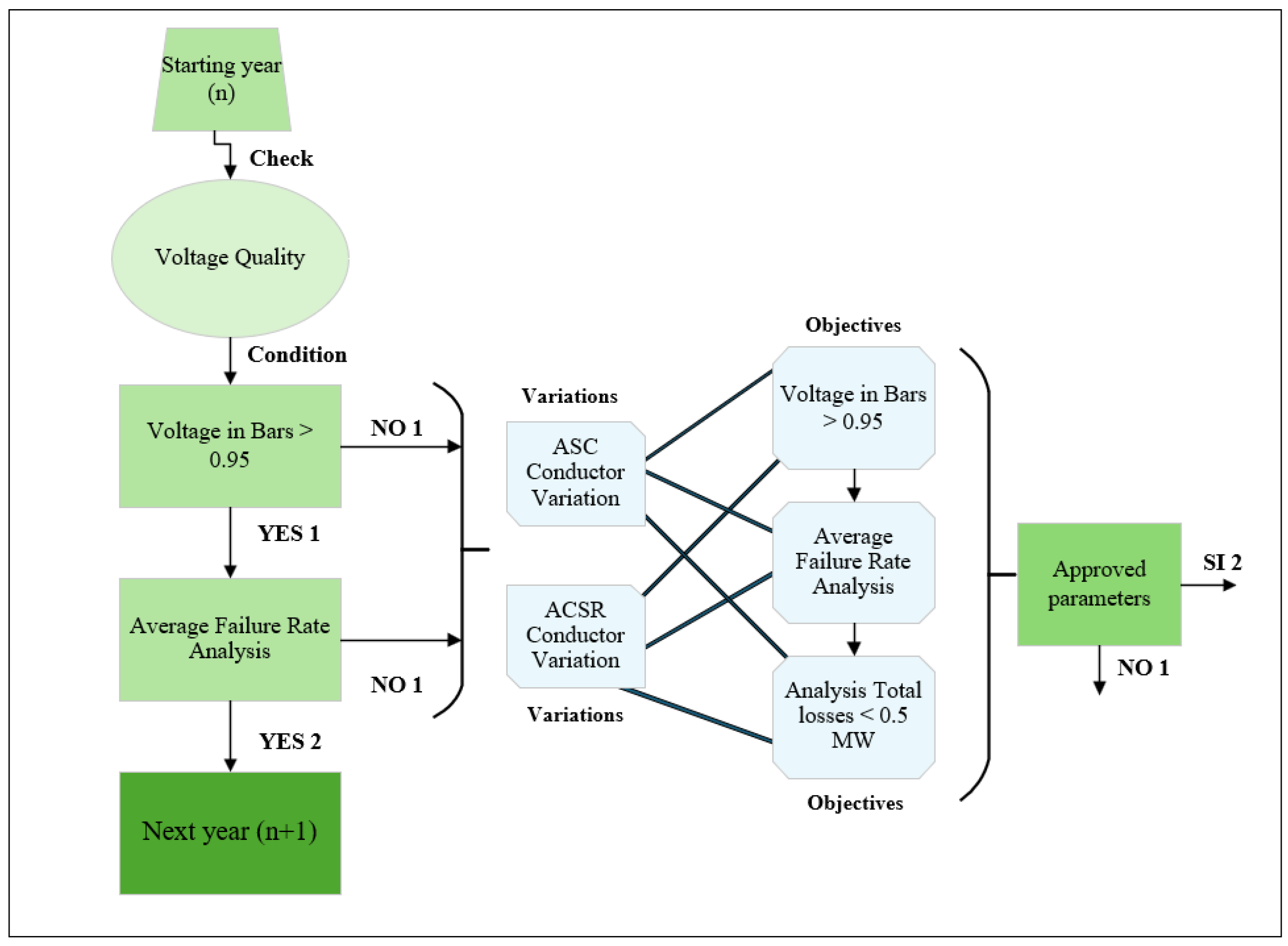
Although five input conditions are considered as valid or positive responses under different scenarios, initial constraints are proposed that must be fulfilled prior to the analysis. These are:
- First constraint: the analysis is carried out only if the voltage at the buses (expressed in p.u.) falls below the established minimum voltage threshold.
- Second constraint: if total system losses exceed 0.5 MW, the analysis is performed.
By considering these constraints as the starting point, the optimization analysis focuses on critical conditions within the system, avoiding unnecessary computation during years in which demand growth does not negatively affect distribution system performance—specifically, when quality and reliability parameters remain above minimum acceptable thresholds. This approach helps reduce unnecessary economic impact associated with premature system upgrades or modifications.
3. Case Study: IEEE 15-Bus Distribution System
The continuous growth in demand causes instability in distribution systems due to their direct connection with end users. Traditional methods propose improving system quality and stability, often through the use of reactive compensation, which is directly injected into the system. However, these approaches tend to overlook the behavior and impact of increasing demand on the components of the distribution network.
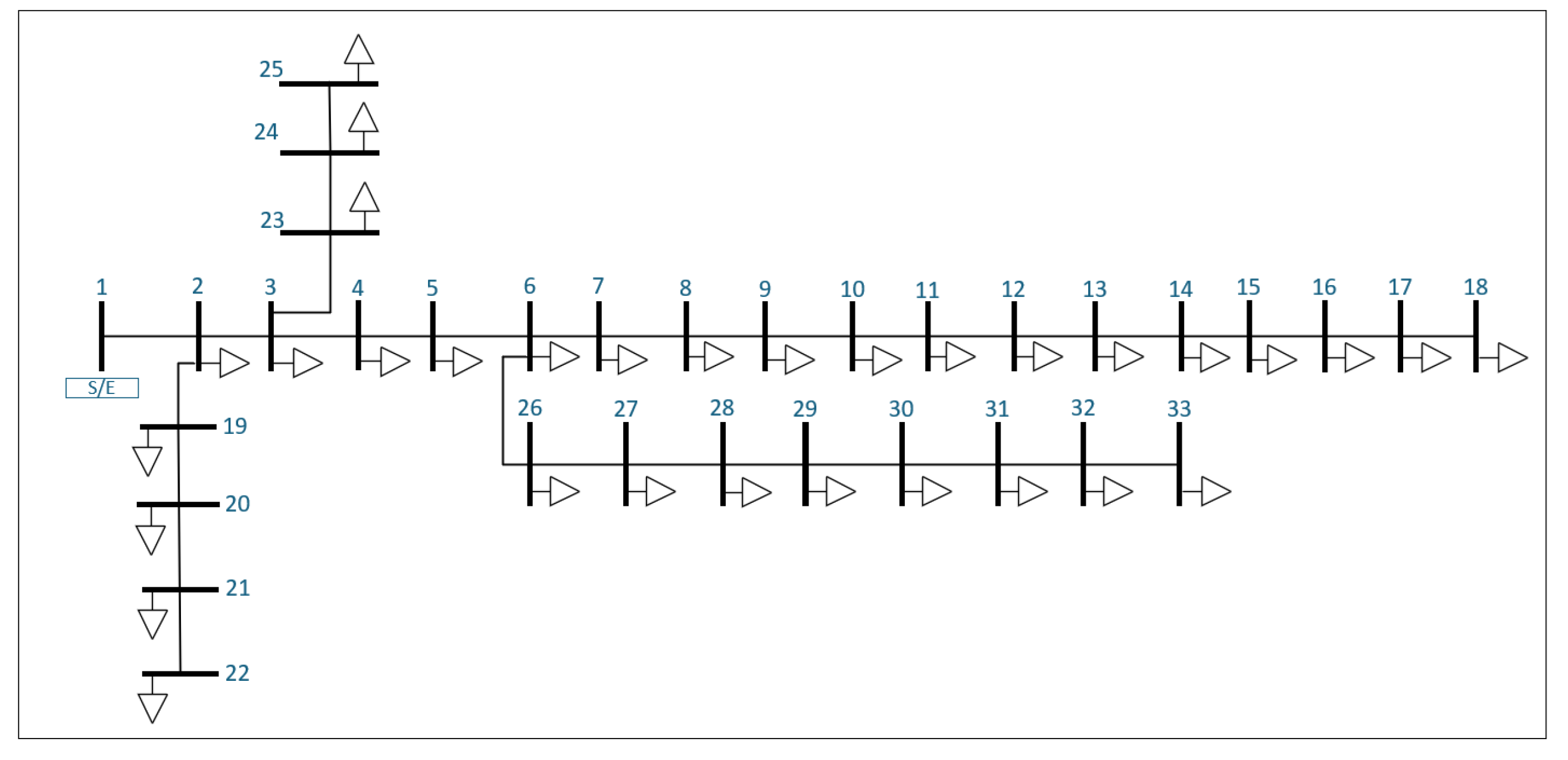
Figure 2.
15-Bus Distribution System.
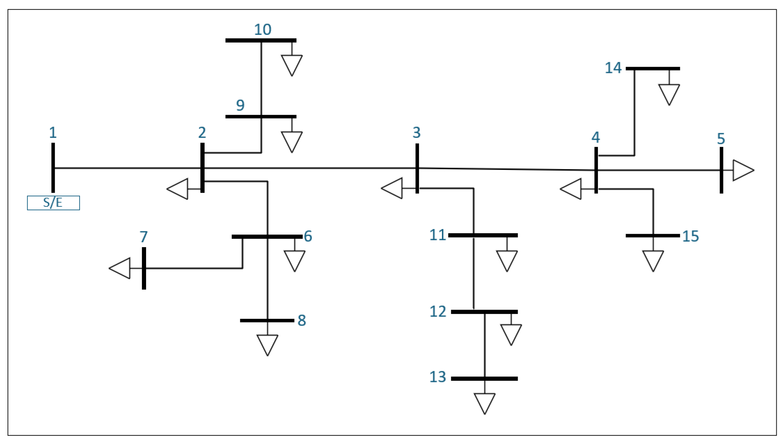
Based on the above, the IEEE 15-bus distribution system template developed by Das D., Kothari D. P., and Kalam A. in 1995 was used. This system offers a simple and effective method for solving radial distribution networks and operates with a base voltage of 13.3 kV.
The following analysis presents a 5% annual demand increase over a 10-year period for the IEEE 15-bus distribution system.

Table 3.
Active Power Growth (MW) in the 15-Bus Distribution System.
| Load | Year 0 | Year 1 | Year 3 | Year 5 | Year 7 | Year 9 | Year 10 |
|---|---|---|---|---|---|---|---|
| Load 1 | 0 | 0 | 0 | 0 | 0 | 0 | 0 |
| Load 2 | 44.1 | 46.305 | 51.051 | 56.284 | 62.053 | 68.414 | 71.834 |
| Load 3 | 70 | 73.5 | 81.034 | 89.34 | 98.497 | 108.593 | 114.023 |
| Load 4 | 140 | 147 | 162.068 | 178.679 | 196.994 | 217.186 | 228.045 |
| Load 5 | 44.1 | 46.305 | 51.051 | 56.284 | 62.053 | 68.414 | 71.834 |
| Load 6 | 140 | 147 | 162.068 | 178.679 | 196.994 | 217.186 | 228.045 |
| Load 7 | 140 | 147 | 162.068 | 178.679 | 196.994 | 217.186 | 228.045 |
| Load 8 | 70 | 73.5 | 81.034 | 89.34 | 98.497 | 108.593 | 114.023 |
| Load 9 | 70 | 73.5 | 81.034 | 89.34 | 98.497 | 108.593 | 114.023 |
| Load 10 | 44.1 | 46.305 | 51.051 | 56.284 | 62.053 | 68.414 | 71.834 |
| Load 11 | 140 | 147 | 162.068 | 178.679 | 196.994 | 217.186 | 228.045 |
| Load 12 | 70 | 73.5 | 81.034 | 89.34 | 98.497 | 108.593 | 114.023 |
| Load 13 | 44.1 | 46.305 | 51.051 | 56.284 | 62.053 | 68.414 | 71.834 |
| Load 14 | 70 | 73.5 | 81.034 | 89.34 | 98.497 | 108.593 | 114.023 |
| Load 15 | 140 | 147 | 162.068 | 178.679 | 196.994 | 217.186 | 228.045 |
Table 4.
Reactive Power Growth (MVAr) in the 15-Bus Distribution System.
| Load | Year 0 | Year 1 | Year 3 | Year 5 | Year 7 | Year 9 | Year 10 |
|---|---|---|---|---|---|---|---|
| Load 1 | 0 | 0 | 0 | 0 | 0 | 0 | 0 |
| Load 2 | 44.991 | 47.24055 | 52.083 | 57.421 | 63.307 | 69.796 | 73.286 |
| Load 3 | 71.4143 | 74.985015 | 82.671 | 91.145 | 100.487 | 110.787 | 116.326 |
| Load 4 | 142.8286 | 149.97003 | 165.342 | 182.29 | 200.974 | 221.574 | 232.653 |
| Load 5 | 44.991 | 47.24055 | 52.083 | 57.421 | 63.307 | 69.796 | 73.286 |
| Load 6 | 142.8286 | 149.97003 | 165.342 | 182.29 | 200.974 | 221.574 | 232.653 |
| Load 7 | 142.8286 | 149.97003 | 165.342 | 182.29 | 200.974 | 221.574 | 232.653 |
| Load 8 | 71.4143 | 74.985015 | 82.671 | 91.145 | 100.487 | 110.787 | 116.326 |
| Load 9 | 71.4143 | 74.985015 | 82.671 | 91.145 | 100.487 | 110.787 | 116.326 |
| Load 10 | 44.991 | 47.24055 | 52.083 | 57.421 | 63.307 | 69.796 | 73.286 |
| Load 11 | 142.8286 | 149.97003 | 165.342 | 182.29 | 200.974 | 221.574 | 232.653 |
| Load 12 | 71.4143 | 74.985015 | 82.671 | 91.145 | 100.487 | 110.787 | 116.326 |
| Load 13 | 44.991 | 47.24055 | 52.083 | 57.421 | 63.307 | 69.796 | 73.286 |
| Load 14 | 71.4143 | 74.985015 | 82.671 | 91.145 | 100.487 | 110.787 | 116.326 |
| Load 15 | 142.8286 | 149.97003 | 165.342 | 182.29 | 200.974 | 221.574 | 232.653 |
4. Results for the 15-Bus Distribution System
The implementation of traditional methods to mitigate the negative impacts caused by demand growth aims to improve the system’s power quality and reliability. However, these methods are often not aligned with the economic impact they entail during implementation. One of the main electrical components affected by increasing demand is the distribution line conductor. Due to its exposure to open air and environmental conditions, it is prone to corrosion or oxidation, which increases resistance to current flow and leads to greater power losses in the system.
Based on the above, and in order to provide a feasible solution to growing demand, modifications to the conductors in the distribution system were carried out to evaluate their performance under voltage quality, loss reduction, and reliability improvement parameters—without resorting to traditional solutions such as capacitor banks, distributed generation, circuit duplication, or any other major system changes.
Table 5.
Losses in the IEEE 15-bus model, Year 0.
| Line | Value | Unit |
|---|---|---|
| L1–L2 | 0.038 | MW |
| L2–L3 | 0.011 | MW |
| L3–L4 | 0.002 | MW |
| L2–L6 | 0.006 | MW |
| L3–L11 | 0.002 | MW |
With the implementation of the multi-criteria function, which includes specific characteristics and constraints, the goal is to offer a technically and economically sustainable solution while maintaining or improving system reliability and power quality. The most relevant modifications applied to the evaluated distribution systems are presented below.
4.1. Initial Conditions (Case 0)
Prior to the development of the multi-criteria function, system parameters under initial conditions were obtained for each distribution model. These included: bus voltage in per unit (p.u.), total system losses in megawatts (MW), and the average failure rate of the conductors. The IEEE 15-bus distribution system shows voltages below the minimum threshold (0.95 p.u.) at buses 12, 13, 14, and 15, making it necessary to apply changes from year zero, as illustrated in Figure 3.
Based on the system loss analysis, the IEEE 15-bus model exhibits a total of 0.06 MW in losses. Notably, the most significant losses occur in the following lines:
To evaluate the system’s reliability, the average failure rate per kilometer of the conductors was assessed. The IEEE 15-bus model shows a failure rate range between 9.56% (minimum) and 13.46% (maximum), particularly in lines L9–L10 and L12–L3.
4.2. Analysis of the 15-Bus Distribution System
Considering voltage quality and system reliability as essential requirements for the distribution system, the multi-criteria function analysis was initiated in year 0. This is because the IEEE 15-bus model exhibited voltages below the minimum permissible threshold (0.95 p.u.), with a base voltage of 13.3 kV.
By applying the multi-criteria function, the conductors in lines L1–L2, L2–L3, L3–L4, L2–L6, L3–L11, and L11–L12 were replaced with the “Iris” type conductor from the ASC or AAC catalog, which has the following characteristics:
- Gauge: 2 AWG.
- Cross-sectional Area: 33.62 mm2.
- Resistance: 0.856 Ohm/km.
- Cost: 0.926 USD/m.
Replacing the conductors in the aforementioned lines improved the voltage profile of the system, reduced total power losses, and decreased the average failure rate within the system.
Figure 4.
Comparison of voltage in p.u. between Year 0 and the condition after replacing conductors in lines L1–L2, L2–L3, L3–L4, L2–L6, L3–L11, and L11–L12.
Figure 4.
Comparison of voltage in p.u. between Year 0 and the condition after replacing conductors in lines L1–L2, L2–L3, L3–L4, L2–L6, L3–L11, and L11–L12.
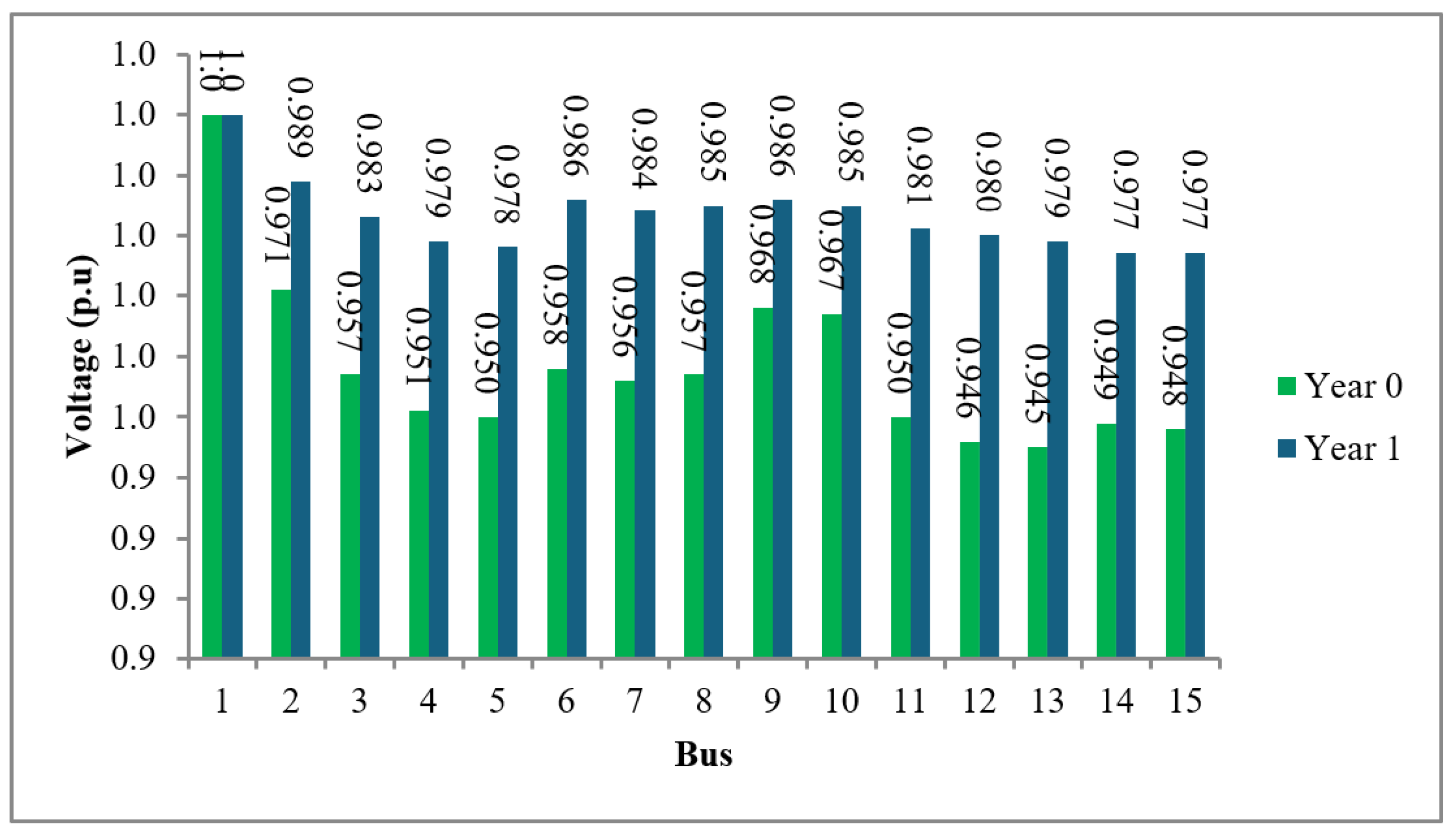
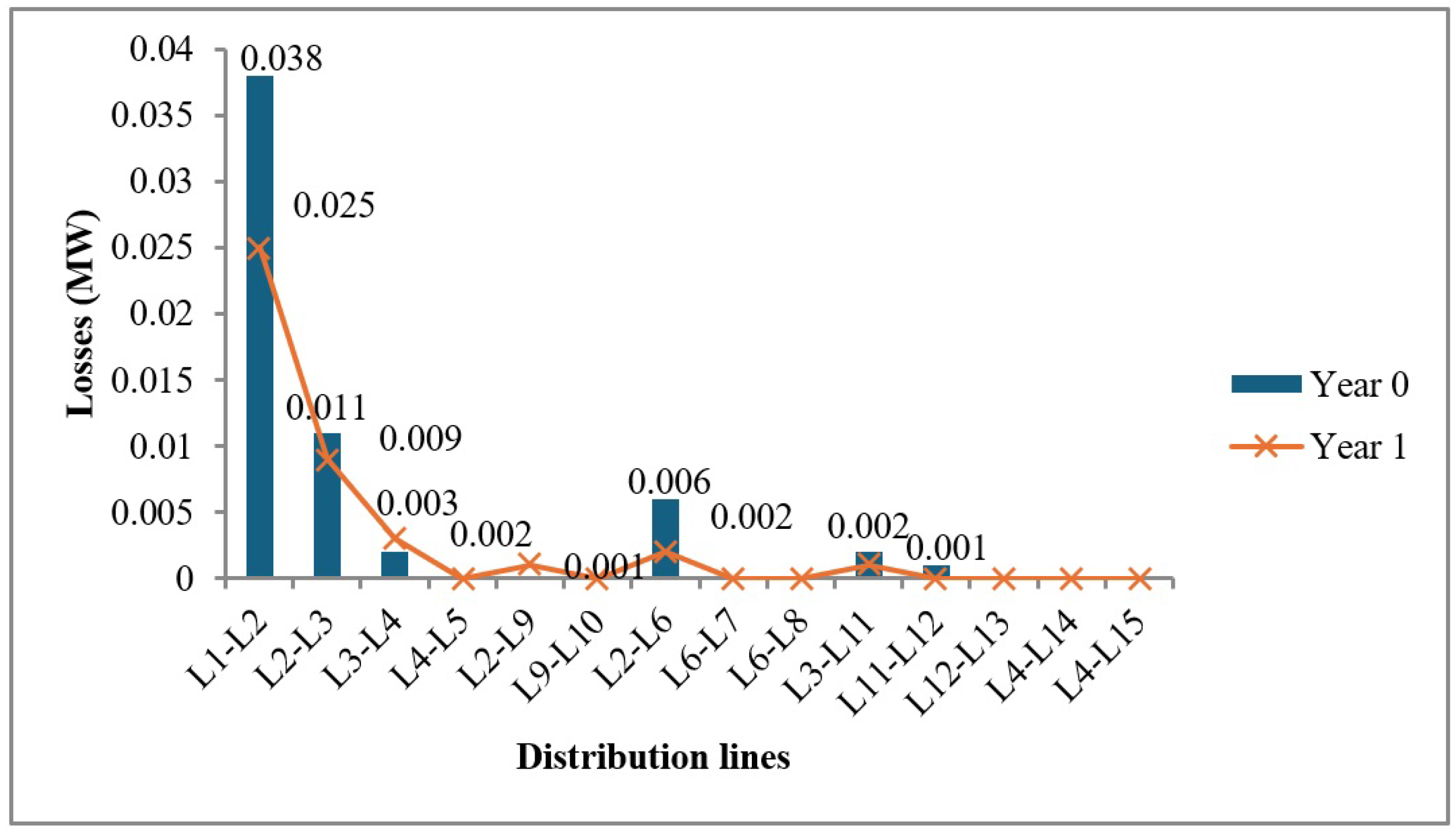
After replacing the conductors in the distribution lines L1–L2, L2–L3, L3–L4, L2–L6, L3–L11, and L11–L12, the total system losses were reduced to 0.041 MW. Likewise, the partial resistances of the replaced lines were lowered.
Figure 5.
Loss comparison: initial 15-bus distribution system (Case 0) vs. the system with replaced conductors.
Figure 5.
Loss comparison: initial 15-bus distribution system (Case 0) vs. the system with replaced conductors.
Similarly, replacing the conductors also resulted in a reduction of the average failure rate throughout the system, as shown in Figure 6.
With the gradual 5% increase in load, no conductor replacements were required in the five years following the initial changes, as the system continued to meet the minimum voltage requirement (0.95 p.u.). It was observed that the next adjustment or conductor replacement should be carried out in year 6. The optimal solution in this case was the replacement of the conductor in distribution line L1–L2 with an ACSR-type conductor, characterized by:
- Gauge: 1/0 AWG.
- Cross-sectional Area: 53.49 mm2.
- Resistance: 0.5227 Ohm/km.
- Cost: 1.24 USD/m.
After performing this replacement and applying the projected load growth for the following four years, it was determined that no further conductor replacements were necessary in the distribution system for any year beyond year 6. The voltage behavior over the final four years is shown in Figure 7.
The following expansion plan summarizes the adjustments made in year 0, including the changes applied to the distribution lines and their direct impact on system power quality and reliability.
Table 6.
Expansion Plan Year 0 – Year 1.
| Reliability Year 0 | Reliability Year 1 | Quality Year 0 and Year 1 | |||||
|---|---|---|---|---|---|---|---|
| Line | Conductor | AFR (%) | Conductor | AFR (%) | Bus | V (p.u) | V (p.u) |
| L1–L2 | ALTON 48.69 | 9.622 | Iris | 6.932 | Bus 1 | 1.00 | 1.00 |
| L2–L3 | SWAN | 11.148 | Iris | 6.828 | Bus 2 | 0.971 | 0.989 |
| L3–L4 | SPARROW | 9.276 | Iris | 9.0108 | Bus 3 | 0.957 | 0.983 |
| L4–L5 | AKRON 4 | 9.626 | AKRON 4 | 9.350 | Bus 4 | 0.951 | 0.979 |
| L2–L9 | TURKEY | 13.283 | TURKEY | 12.905 | Bus 5 | 0.950 | 0.978 |
| L9–L10 | AKRON 4 | 9.566 | AKRON 4 | 9.293 | Bus 6 | 0.958 | 0.986 |
| L2–L6 | AKRON 6 | 11.270 | Iris | 4.331 | Bus 7 | 0.956 | 0.984 |
| L6–L7 | SWAN | 11.022 | SWAN | 10.820 | Bus 8 | 0.957 | 0.985 |
| L6–L8 | SWAN | 11.033 | SWAN | 10.831 | Bus 9 | 0.968 | 0.986 |
| L3–L11 | AKRON | 9.636 | Iris | 5.864 | Bus 10 | 0.967 | 0.985 |
| L11–L12 | AKRON | 11.401 | Iris | 4.354 | Bus 11 | 0.950 | 0.981 |
| L12–L13 | TURKEY | 13.465 | TURKEY | 12.998 | Bus 12 | 0.946 | 0.980 |
| L4–L14 | AKRON 6 | 11.365 | AKRON 6 | 11.040 | Bus 13 | 0.945 | 0.979 |
| L4–L15 | SWAN | 11.254 | SWAN | 10.9206 | Bus 14 | 0.949 | 0.977 |
| – | – | – | – | – | Bus 15 | 0.948 | 0.977 |
The adjustments made in year 0 ensure adequate power quality and reliability until the projected demand growth scenario in year 6, when the next system enhancement is recommended. The following table presents the expansion plan between years 6 and 7.
Table 7.
Expansion Plan Year 6 – Year 7.
| Reliability Year 6 | Reliability Year 7 | Quality Year 6 and Year 7 | |||||
|---|---|---|---|---|---|---|---|
| Line | Conductor | AFR (%) | Conductor | AFR (%) | Bus | V (p.u) | V (p.u) |
| L1–L2 | Iris | 8.032 | Raven | 7.642 | Bus 1 | 1.00 | 1.00 |
| L2–L3 | Iris | 7.920 | Iris | 7.530 | Bus 2 | 0.986 | 0.990 |
| L3–L4 | Iris | 10.452 | Iris | 10.062 | Bus 3 | 0.978 | 0.982 |
| L4–L5 | AKRON 4 | 9.408 | AKRON 4 | 9.370 | Bus 4 | 0.9740 | 0.977 |
| L2–L9 | TURKEY | 12.945 | TURKEY | 12.905 | Bus 5 | 0.972 | 0.976 |
| L9–L10 | AKRON 4 | 9.331 | AKRON 4 | 9.303 | Bus 6 | 0.983 | 0.986 |
| L2–L6 | Iris 6 | 5.0198 | Iris | 4.619 | Bus 7 | 0.980 | 0.983 |
| L6–L7 | SWAN | 10.865 | SWAN | 10.820 | Bus 8 | 0.981 | 0.984 |
| L6–L8 | SWAN | 10.876 | SWAN | 10.842 | Bus 9 | 0.982 | 0.986 |
| L3–L11 | Iris | 3.705 | Raven | 2.963 | Bus 10 | 0.981 | 0.984 |
| L11–L12 | Iris | 4.380 | Iris | 3.962 | Bus 11 | 0.976 | 0.979 |
| L12–L13 | TURKEY | 13.078 | TURKEY | 13.038 | Bus 12 | 0.974 | 0.978 |
| L4–L14 | AKRON 6 | 11.108 | AKRON 6 | 11.014 | Bus 13 | 0.973 | 0.976 |
| L4–L15 | SWAN | 10.99 | SWAN | 10.954 | Bus 14 | 0.971 | 0.974 |
| – | – | – | – | – | Bus 15 | 0.970 | 0.974 |
5. Case Study: 33-Bus Distribution System
The 33-bus distribution system, developed by Kashem M. A., Ganapathy V., Jasmon G. B., and Buhari M. in the year 2000, presents a method for minimizing losses in distribution networks. This system operates with a base voltage of 12.66 kV.
Figure 8.
33-Bus Distribution System.
A 5% annual increase in demand was applied over a 10-year period in the 33-bus distribution system.
Table 8.
Active Power Growth (MW) in the 33-Bus Distribution System.
| Load | Year 0 | Year 1 | Year 3 | Year 5 | Year 7 | Year 9 | Year 10 |
|---|---|---|---|---|---|---|---|
| Load 1 | 0 | 0 | 0 | 0 | 0 | 0 | 0 |
| Load 2 | 100 | 105 | 115.76 | 127.63 | 140.71 | 155.13 | 162.89 |
| Load 3 | 90 | 94.5 | 104.19 | 114.87 | 126.64 | 139.62 | 146.6 |
| Load 4 | 120 | 126 | 138.92 | 153.15 | 168.85 | 186.16 | 195.47 |
| Load 5 | 60 | 63 | 69.46 | 76.58 | 84.43 | 93.08 | 97.73 |
| Load 6 | 60 | 63 | 69.46 | 76.58 | 84.43 | 93.08 | 97.73 |
| Load 7 | 200 | 210 | 231.53 | 255.26 | 281.42 | 310.27 | 325.78 |
| Load 8 | 200 | 210 | 231.53 | 255.26 | 281.42 | 310.27 | 325.78 |
| Load 9 | 60 | 63 | 69.46 | 76.58 | 84.43 | 93.08 | 97.73 |
| Load 10 | 60 | 63 | 69.46 | 76.58 | 84.43 | 93.08 | 97.73 |
| Load 11 | 45 | 47.25 | 52.09 | 57.43 | 63.32 | 69.81 | 73.3 |
| Load 12 | 60 | 63 | 69.46 | 76.58 | 84.43 | 93.08 | 97.73 |
| Load 13 | 60 | 63 | 69.46 | 76.58 | 84.43 | 93.08 | 97.73 |
| Load 14 | 120 | 126 | 138.92 | 153.15 | 168.85 | 186.16 | 195.47 |
| Load 15 | 60 | 63 | 69.46 | 76.58 | 84.43 | 93.08 | 97.73 |
| Load 16 | 60 | 63 | 69.46 | 76.58 | 84.43 | 93.08 | 97.73 |
| Load 17 | 60 | 63 | 69.46 | 76.58 | 84.43 | 93.08 | 97.73 |
| Load 18 | 90 | 94.5 | 104.19 | 114.87 | 126.64 | 139.62 | 146.6 |
| Load 19 | 90 | 94.5 | 104.19 | 114.87 | 126.64 | 139.62 | 146.6 |
| Load 20 | 90 | 94.5 | 104.19 | 114.87 | 126.64 | 139.62 | 146.6 |
| Load 21 | 90 | 94.5 | 104.19 | 114.87 | 126.64 | 139.62 | 146.6 |
| Load 22 | 90 | 94.5 | 104.19 | 114.87 | 126.64 | 139.62 | 146.6 |
| Load 23 | 90 | 94.5 | 104.19 | 114.87 | 126.64 | 139.62 | 146.6 |
| Load 24 | 420 | 441 | 486.2 | 536.04 | 590.98 | 651.56 | 684.14 |
| Load 25 | 420 | 441 | 486.2 | 536.04 | 590.98 | 651.56 | 684.14 |
| Load 26 | 60 | 63 | 69.46 | 76.58 | 84.43 | 93.08 | 97.73 |
| Load 27 | 60 | 63 | 69.46 | 76.58 | 84.43 | 93.08 | 97.73 |
| Load 28 | 60 | 63 | 69.46 | 76.58 | 84.43 | 93.08 | 97.73 |
| Load 29 | 120 | 126 | 138.92 | 153.15 | 168.85 | 186.16 | 195.47 |
| Load 30 | 200 | 210 | 231.53 | 255.26 | 281.42 | 310.27 | 325.78 |
| Load 31 | 150 | 157.5 | 173.64 | 191.44 | 211.07 | 232.7 | 244.33 |
| Load 32 | 210 | 220.5 | 243.1 | 268.02 | 295.49 | 325.78 | 342.07 |
| Load 33 | 60 | 63 | 69.46 | 76.58 | 84.43 | 93.08 | 97.73 |
The objective is to generate various case studies based on the IEEE 33-bus distribution system by identifying the specific data of the electrical components. Then, using the multi-criteria function, optimal results are obtained by considering key parameters such as resistance, power losses, economic impact, voltage deviation, and average failure rate.
Table 9.
Reactive Power Growth (MVAr) in the 33-Bus Distribution System.
| Load | Year 0 | Year 1 | Year 3 | Year 5 | Year 7 | Year 9 | Year 10 |
|---|---|---|---|---|---|---|---|
| Load 1 | 0 | 0 | 0 | 0 | 0 | 0 | 0 |
| Load 2 | 60 | 63 | 69.46 | 76.58 | 84.43 | 93.08 | 97.73 |
| Load 3 | 40 | 42 | 46.31 | 51.05 | 56.28 | 62.05 | 65.16 |
| Load 4 | 80 | 84 | 92.61 | 102.1 | 112.57 | 124.11 | 130.31 |
| Load 5 | 30 | 31.5 | 34.73 | 38.29 | 42.21 | 46.54 | 48.87 |
| Load 6 | 20 | 21 | 23.15 | 25.53 | 28.14 | 31.03 | 32.58 |
| Load 7 | 100 | 105 | 115.76 | 127.63 | 140.71 | 155.13 | 162.89 |
| Load 8 | 100 | 105 | 115.76 | 127.63 | 140.71 | 155.13 | 162.89 |
| Load 9 | 20 | 21 | 23.15 | 25.53 | 28.14 | 31.03 | 32.58 |
| Load 10 | 20 | 21 | 23.15 | 25.53 | 28.14 | 31.03 | 32.58 |
| Load 11 | 30 | 31.5 | 34.73 | 38.29 | 42.21 | 46.54 | 48.87 |
| Load 12 | 35 | 36.75 | 40.52 | 44.67 | 49.25 | 54.3 | 57.01 |
| Load 13 | 35 | 36.75 | 40.52 | 44.67 | 49.25 | 54.3 | 57.01 |
| Load 14 | 80 | 84 | 92.61 | 102.1 | 112.57 | 124.11 | 130.31 |
| Load 15 | 10 | 10.5 | 11.58 | 12.76 | 14.07 | 15.51 | 16.29 |
| Load 16 | 20 | 21 | 23.15 | 25.53 | 28.14 | 31.03 | 32.58 |
| Load 17 | 20 | 21 | 23.15 | 25.53 | 28.14 | 31.03 | 32.58 |
| Load 18 | 40 | 42 | 46.31 | 51.05 | 56.28 | 62.05 | 65.16 |
| Load 19 | 40 | 42 | 46.31 | 51.05 | 56.28 | 62.05 | 65.16 |
| Load 20 | 40 | 42 | 46.31 | 51.05 | 56.28 | 62.05 | 65.16 |
| Load 21 | 40 | 42 | 46.31 | 51.05 | 56.28 | 62.05 | 65.16 |
| Load 22 | 40 | 42 | 46.31 | 51.05 | 56.28 | 62.05 | 65.16 |
| Load 23 | 50 | 52.5 | 57.88 | 63.81 | 70.36 | 77.57 | 81.44 |
| Load 24 | 200 | 210 | 231.53 | 255.26 | 281.42 | 310.27 | 325.78 |
| Load 25 | 200 | 210 | 231.53 | 255.26 | 281.42 | 310.27 | 325.78 |
| Load 26 | 25 | 26.25 | 28.94 | 31.91 | 35.18 | 38.78 | 40.72 |
| Load 27 | 25 | 26.25 | 28.94 | 31.91 | 35.18 | 38.78 | 40.72 |
| Load 28 | 20 | 21 | 23.15 | 25.53 | 28.14 | 31.03 | 32.58 |
| Load 29 | 70 | 73.5 | 81.03 | 89.34 | 98.5 | 108.59 | 114.02 |
| Load 30 | 600 | 630 | 694.58 | 765.77 | 844.26 | 930.8 | 977.34 |
| Load 31 | 70 | 73.5 | 81.03 | 89.34 | 98.5 | 108.59 | 114.02 |
| Load 32 | 100 | 105 | 115.76 | 127.63 | 140.71 | 155.13 | 162.89 |
| Load 33 | 40 | 42 | 46.31 | 51.05 | 56.28 | 62.05 | 65.16 |
6. Results for the 33-Bus Distribution System
The analysis of the multi-criteria function depends on the input data and existing constraints in the distribution system. Therefore, an initial analysis of the IEEE 33-bus system is conducted to assess its behavior throughout the demand growth period.
6.1. Initial Conditions (Case 0)
Since the IEEE 33-bus distribution system does not exhibit voltages below the minimum threshold (0.95 p.u.), and the voltage quality parameter remains above the established minimum, it is not necessary to conduct a voltage quality analysis for year 0. The minimum voltage recorded is 1.014 p.u. at bus 18, as shown in Figure 9.
The IEEE 33-bus model satisfies the voltage quality requirements for year 0, and the total power losses (0.168 MW) remain below expected limits. Thus, a full loss analysis is not required for this year. However, the most significant losses are presented in the following table:
Table 10.
Losses in the IEEE 33-bus model, Year 0.
| Line | Value | Unit |
|---|---|---|
| L2–L3 | 0.038 | MW |
| L5–L6 | 0.011 | MW |
| L4–L5 | 0.002 | MW |
| L3–L4 | 0.006 | MW |
To assess the system’s reliability conditions, the average failure rate per kilometer was evaluated. The IEEE 33-bus model shows a range between 5.62% (minimum) and 14.29% (maximum), with the most affected lines being L1–L2 and L21–L8.
6.2. Analysis of the 33-Bus Distribution System
Since the IEEE 33-bus distribution system maintains voltage levels above the minimum threshold (0.95 p.u.) in year 0, a 5% increase in load was applied each year. As the years progressed, the voltage did not fall below the minimum threshold, thus voltage quality remained compliant. Therefore, the system losses were analyzed instead, and in year 8, conductor replacements were deemed necessary in the following lines: L7–L8, L9–L10, L12–L13, L16–L17, L19–L20, and L27–L28. These lines were replaced with the following ASC or AAC-type conductor:
- Gauge: 2 AWG
- Cross-sectional Area: 33.62 mm2
- Resistance: 0.856 Ohm/km
- Cost: 0.926 USD/m
The replacement of the above-mentioned conductors in the specified distribution lines led to an improvement in the voltage profile at buses 10, 11, 12, 13, 14, 15, 16, 17, 18, 20, 21, and 22, as illustrated in Figure 10.
The total power losses in the IEEE 33-bus distribution system in year 8 reached 0.411 MW. After the conductor replacements in the specified lines, total losses in year 9 decreased to 0.394 MW. Likewise, the maximum average failure rate per kilometer in year 8 was 11.21% in the previously mentioned lines. In year 9, after replacing the conductors, this value was reduced to 7.05%.
The following table presents the expansion plan reflecting the most relevant changes implemented in year 8. It highlights the improvements in power quality and system reliability resulting from the conductor replacements.
Table 11.
Expansion Plan Year 8 – Year 9.
| Reliability Year 8 | Reliability Year 9 | Quality Year 8 and Year 9 | |||||
|---|---|---|---|---|---|---|---|
| Line | Conductor | AFR (%) | Conductor | AFR (%) | Bus | V (p.u) | V (p.u) |
| L7–L8 | SWAN | 11.968 | Iris | 7.529 | Bus 8 | 1.007 | 1.013 |
| L9–L10 | SWAN | 12.304 | Iris | 7.740 | Bus 9 | 0.998 | 1.004 |
| L12–L13 | SWAN | 12.441 | Iris | 7.826 | Bus 12 | 0.997 | 0.994 |
| L16–L17 | SWAN | 12.633 | Iris | 7.947 | Bus 13 | 0.979 | 0.989 |
| L19–L20 | SWAN | 11.214 | Iris | 7.054 | Bus 14 | 0.975 | 0.986 |
| L27–L28 | SWAN | 11.980 | Iris | 7.536 | Bus 15 | 0.973 | 0.984 |
| – | – | – | – | – | Bus 16 | 0.972 | 0.982 |
| – | – | – | – | – | Bus 17 | 0.969 | 0.980 |
7. Discussion
The continuous growth in energy demand generates significant stress on distribution systems, directly affecting the quality and reliability of the electrical service provided to end users. In response, electrical engineers typically propose various conventional solutions such as the injection of reactive components, the incorporation of distributed generation, or the upgrade of existing infrastructure. However, these approaches, while technically effective, often fail to account for their economic implications, resulting in a considerable financial burden that is ultimately transferred to consumers.
Given this situation, it becomes essential to explore alternative strategies that can mitigate the impact of demand growth while minimizing investment costs, without compromising system performance in terms of power quality and reliability. The development and application of a multi-criteria decision-making (MCDM) approach allows for the integration of multiple technical and economic variables and constraints into a single optimization framework. By accurately defining input parameters and restrictions, the MCDM method yields optimal solutions tailored to the evolution of demand, enabling decision-making that is both technically viable and economically sustainable. This approach offers a promising alternative to traditional methods, as it balances performance enhancement with cost-effectiveness in the management of distribution networks.
8. Conclusions
The planning of distribution system expansion with a focus on voltage quality and reliability is crucial for ensuring long-term efficiency, resilience, and service continuity. Integrating these criteria into system design and decision-making processes enables a more adaptive and robust energy infrastructure—one capable of meeting increasing demand while minimizing losses, maintaining voltage stability, and optimizing resource utilization. This comprehensive approach, supported by advanced modeling techniques and effective system management, is vital to addressing future energy challenges and improving end-user satisfaction.
In this study, two standardized IEEE distribution models—15-bus and 33-bus systems—were analyzed using load flow simulations to extract key electrical parameters including bus voltages, associated loads, line resistances, and base voltage levels (13.3 kV and 12.66 kV respectively). These parameters facilitated the calculation of current through each line and the estimation of the average failure rate per kilometer, a critical reliability indicator.
To simulate real-world scenarios, a projected annual demand growth of 5% was applied to both systems over a 10-year horizon. As expected, the results revealed a progressive degradation of voltage quality, an increase in system losses, and a decline in overall reliability as demand increased. These trends highlighted the need for strategic system upgrades and enabled the definition of a structured optimization strategy through multi-criteria analysis.
For the IEEE 15-bus system, the demand growth necessitated early action. In year 0, conductor replacements were applied to lines L1–L2, L2–L3, L3–L4, L2–L6, L3–L11, and L11–L12 using a type "Iris" conductor. This intervention significantly improved the voltage profile, reduced power losses, and decreased failure rates. For instance, the voltage at buses 3, 4, 5, 12, 13, 14, and 15 improved from initial values of 0.957, 0.951, 0.950, 0.946, 0.945, 0.949, and 0.948 p.u to 0.983, 0.979, 0.978, 0.980, 0.979, 0.977, and 0.977 p.u, respectively. Likewise, losses in key lines such as L1–L2 and L2–L3 decreased from 0.038 MW and 0.011 MW to 0.025 MW and 0.009 MW, respectively. Average failure rates in the same lines also declined, for example, L1–L2 from 9.622% to 6.932%, and L3–L11 from 9.636% to 5.864%.
For the 33-bus system, the MCDM analysis revealed that no immediate action was required during the early years, as voltage levels and system losses remained within acceptable limits. However, by year 8, an increase in total losses to 0.411 MW and high failure rates in certain lines prompted a targeted expansion plan. Conductor replacements were carried out in lines L7–L8, L9–L10, L12–L13, L16–L17, L19–L20, and L27–L28. These actions resulted in voltage improvements at buses 13–17 from initial values of 0.979, 0.975, 0.973, 0.972, and 0.969 p.u to 0.989, 0.986, 0.984, 0.982, and 0.980 p.u, respectively. Additionally, average failure rates in the affected lines were reduced significantly, e.g., L9–L10 from 12.304% to 7.740%, and L19–L20 from 11.214% to 7.054%.
In summary, the application of a multi-criteria optimization strategy allowed for cost-effective and technically sound decisions regarding system reinforcement. The case studies demonstrated the feasibility of improving distribution system performance by optimizing conductor selection and timing of upgrades, ultimately ensuring the maintenance of power quality and system reliability under increasing demand scenarios.
References
- Juan Noh; Wookyu Chae; Woohyun Kim; Sungyun Choi. A Study on Meshed Distribution System and Protection Coordination Using HILS System. ICTC 2022, 13, 344–346. [Google Scholar]
- Xiang Cai; Xiudong Zhou; Qingjun Huang; Junwei Zhu; Ziang Li; Zehong Chen. Low Voltage Governance in Distribution Networks Based on Wide Range On-load Regulating Transformer. ICED 2022, 9, 164–167. [Google Scholar]
- Naoyuki Takahashi; Yokosuka - Shi. Advanced Autonomous Voltage-Control Method using Sensor Data in a Distribution Power System. UTC 2023, 3, 2–6. [Google Scholar]
- Tao Yan; Rui Li; Wei Liu; Wei Zhang; Hui Hui; Yuan Yao. Resiliency Evaluation of Low- Voltage Distribution System Considering Refusal and Misoperation ISPEC 2021, 11, 1425–1429.
- Lisheng Li; Linli Zhang; Yong Sun; Jianxiu Li. Study on Voltage Control in Distribution Network with Renewable Energy Integration UTC 2023, 3, 2–4.
- Liu Haitao; He Lianjie; Li Yuling; Yu Xia. A primary and secondary equipment integrated intelligent distribution system breaker to better locate and isolate faults ICED 2022, 9, 1652–1655.
- Anabel Lemus; Diego Carrión; Eduar Aguirre; Jorge Gonzáles. Localización de recursos distribuidos en redes eléctricas rurales-urbanas marginales considerando el índice de predicción de colapso de tensión INGEIUS 2022.
- Mehdi Attar; Omid Homaee; Sami Repo. Importance Investigation of Load Models Consideration in Stand Alone Voltage Regulators Placementin Distribution Systems. IEEE, 2020.
- Ahmed Bedawy; Karar Mahmoud; Yutaka Sasaki; Yoshifumi Zoka. A Cooperative Voltage Control Approach for Distribution Systems Based on Voltage Regulators and PV Inverters MEPCON 2021.
- Saced Mahdavian; Mohsen Hamzeh. Reactive Power Management of PV Systems by Distributed Cooperative Control in Low Voltage Distribution Networks IEEE 2021.
- Julie Richmond; Liam Mcsweeney; Jonathan Berry. THE OPERATION AND BENEFITS OF AN INTEGRATED NETWORK MODEL TO ENABLE DISTRIBUTION SYSTEM OPERATION CIRED 2021, 9, 0903.
- Santiago Marcial; Alexander Águila. Óptima Compensación de Potencia Reactiva en Redes de Distribución Radiales considerando periodo de diseño INCISCOS 2020, 112–114.
- Diego Ponce; Alexander Águila; Narayanan Krishnan. Optimal Selection of Conductors in Distribution System Designs Using Multi-Criteria Decision MDPI 2023, 9, 6–17.
- Siguencia Oscar; Pires Luis; Sempertegui Rodrigo. Metodologías de decisión multicriterio para planeación energética en zonas rurales del Ecuador I+D+Ingeniería 2021, 8, 293–296.
- Alexander Téllez. Multicriteria Analysis for Quality and Reliability in Electrical Systems 2020, 9, 56–75.
- Alexander Aguila; Leony Ortiz; Rogelio Orizondo; Gabriel López. Optimal location and dimensioning of capacitors in microgrids using a multicriteria decision algorithm Heliyon 7 2021, 3–8.
- Alexander Aguila. OPTIMIZACIÓN MULTICRITERIO DE FLUJOS DE POTENCIA REACTIVA EN SISTEMAS ELÉCTRICOS DE DISTRIBUCIÓN. Universidad Pontificia Bolivariana, 2021.
- Alexander Aguila; Leony Ortiz; Milton Ruiz; K. Narayanan; Silvana Varela. Optimal Location of Reclosers in Electrical Distribution Systems Considering Multicriteria Decision Through the Generation of Scenarios Using the Montecarlo Method. IEE Access, 2023.
- Edison Guanochanga; Alexander Aguila; Leony Ortiz. Multicriteria analysis for optimal reconfiguration of a distribution network in case of failures Heliyon 9 2023.
Figure 3.
Voltage profile in p.u. of the IEEE 15-bus distribution system, Case 0.
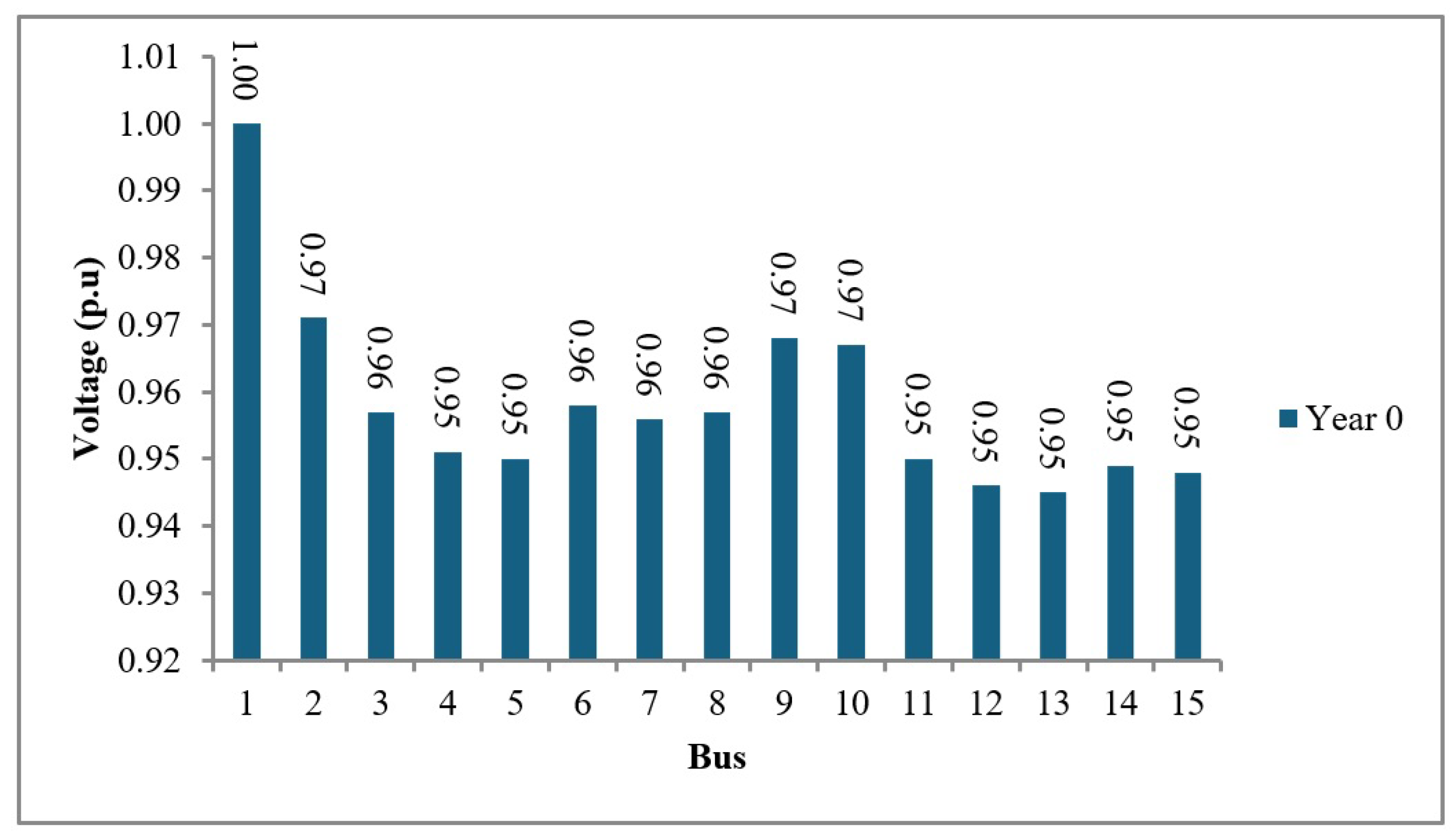
Figure 6.
Average failure rate analysis: Case 0 vs. optimized system with conductor replacements.
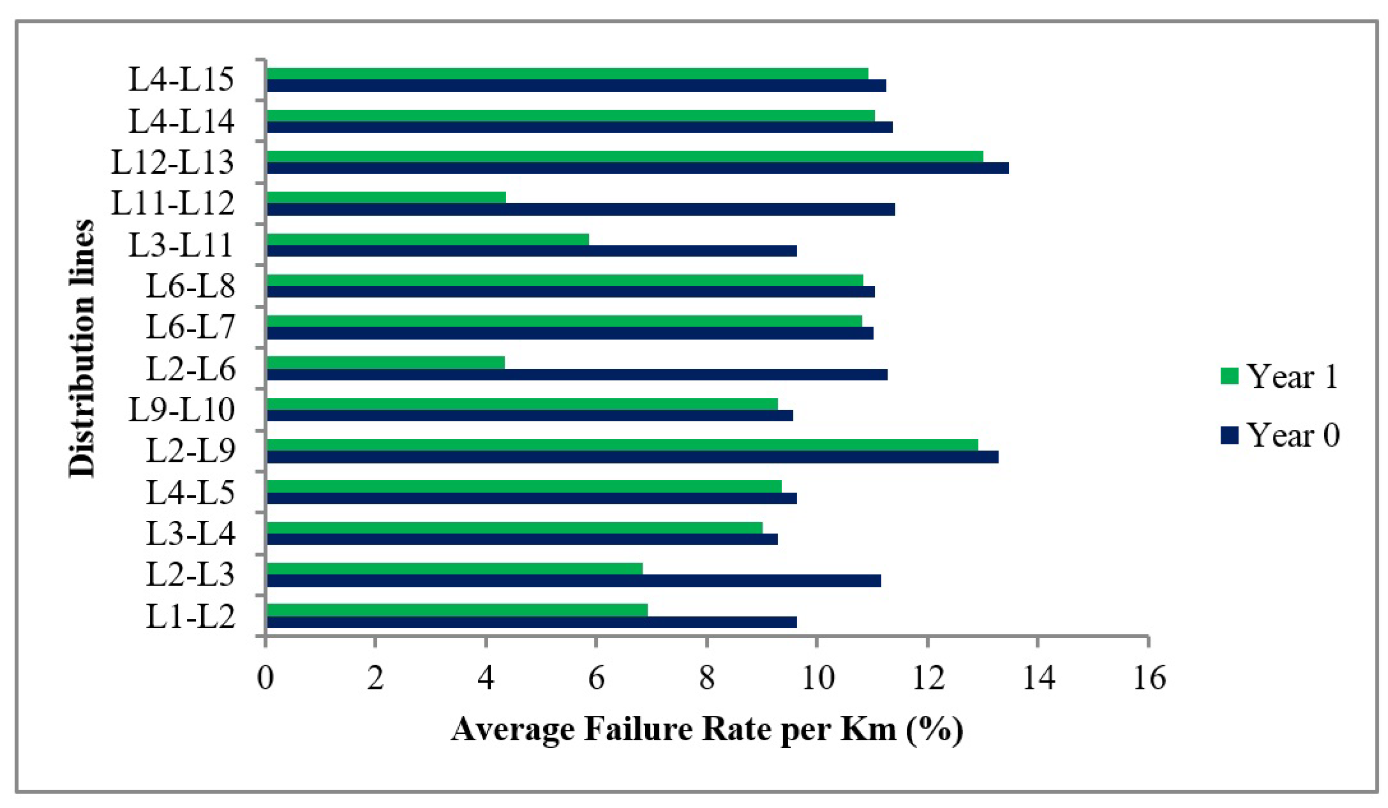
Figure 7.
Voltage behavior in the distribution system under the expansion plan.
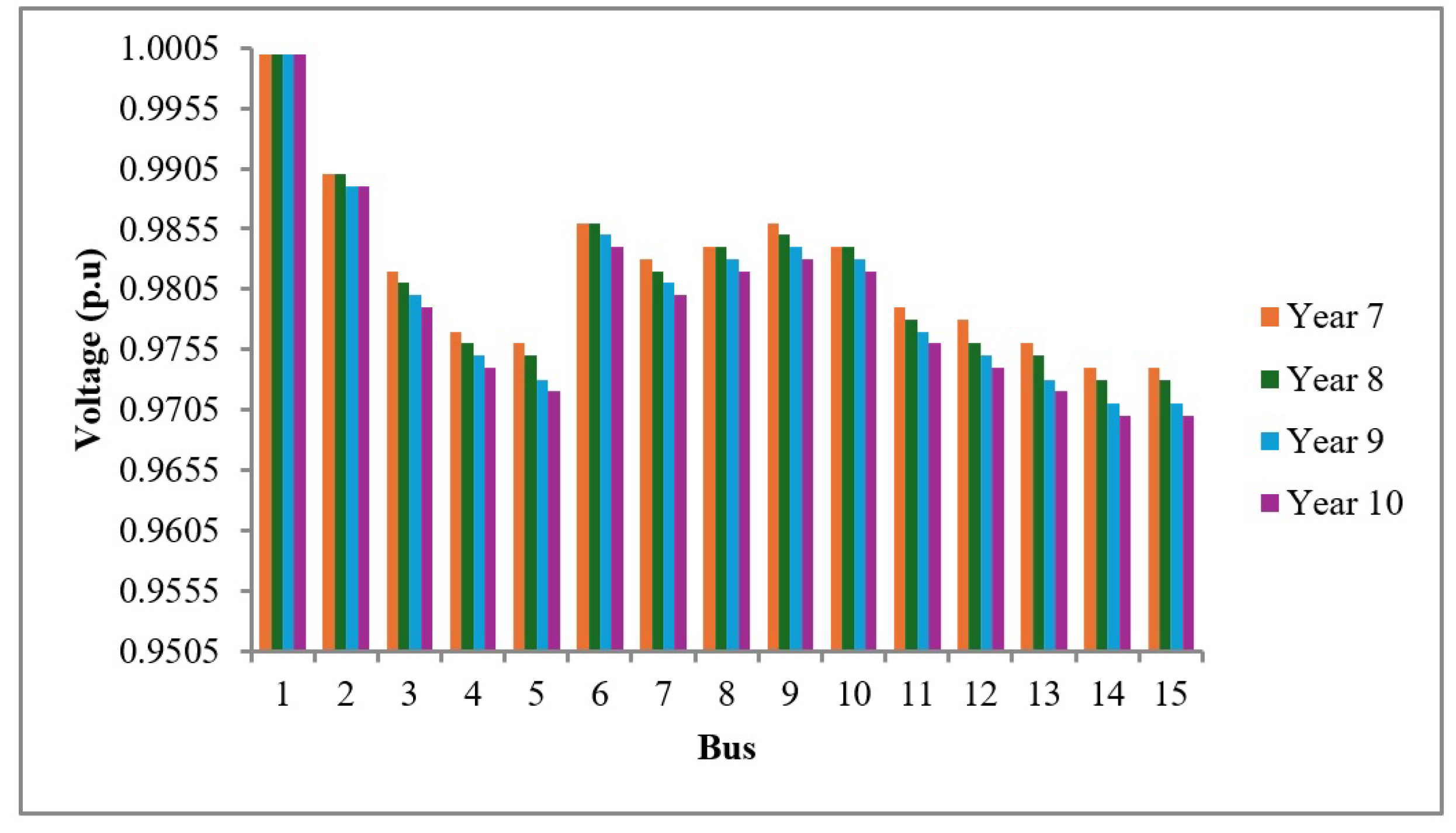
Figure 9.
Voltage in p.u. for the IEEE 33-bus distribution system, Case 0.
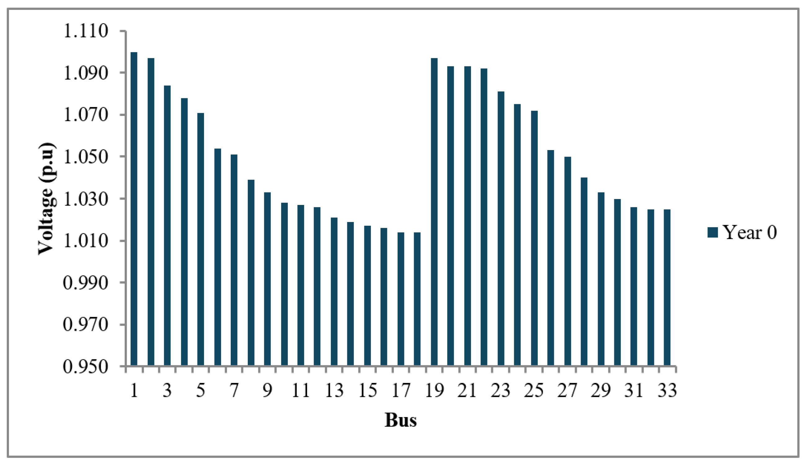
Figure 10.
Voltage comparison in p.u.: Year 8 vs. Year 9.
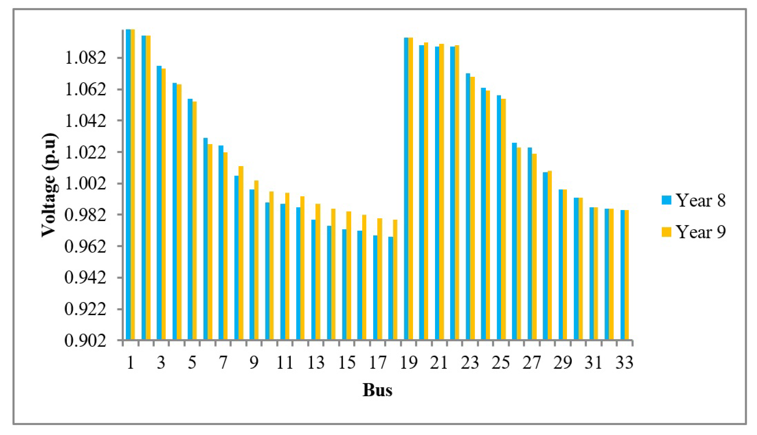
Table 1.
Electrical conductor data for ASC or AAC model.
| Code | Gauge (AWG) | Cross-Sectional Area (mm2) | Resistance (Ohm/Km) | Price (USD/m) |
|---|---|---|---|---|
| Peachbell | 6 | 13.3 | 2.170 | 0.366 |
| Rose | 4 | 21.15 | 1.360 | 0.582 |
| Iris | 2 | 33.62 | 0.856 | 0.926 |
| Poppy | 1/0 | 53.49 | 0.538 | 1.472 |
| Aster | 2/0 | 67.44 | 0.427 | 1.857 |
| Phlox | 3/0 | 85.02 | 0.338 | 2.339 |
| Oxlip | 4/0 | 107.2 | 0.269 | 2.9521 |
1 Obtained from the conductor catalog (ELECTRO CABLES).
Table 2.
Electrical conductor data for ACSR model.
| Code | Gauge (AWG) | Cross-Sectional Area (mm2) | Resistance (Ohm/Km) | Price (USD/m) |
|---|---|---|---|---|
| Turkey | 6 | 13.3 | 2.1065 | 0.37 |
| Swan | 4 | 21. |
Disclaimer/Publisher’s Note: The statements, opinions and data contained in all publications are solely those of the individual author(s) and contributor(s) and not of MDPI and/or the editor(s). MDPI and/or the editor(s) disclaim responsibility for any injury to people or property resulting from any ideas, methods, instructions or products referred to in the content. |
© 2025 by the authors. Licensee MDPI, Basel, Switzerland. This article is an open access article distributed under the terms and conditions of the Creative Commons Attribution (CC BY) license (http://creativecommons.org/licenses/by/4.0/).
Copyright: This open access article is published under a Creative Commons CC BY 4.0 license, which permit the free download, distribution, and reuse, provided that the author and preprint are cited in any reuse.


