1. Introduction
Protecting individuals and the environment from hydrogeological risks represents a formidable challenge within the framework of slope stability, particularly rapid over these years of extreme weather events and climate change. Increasing temperatures, permafrost thaw, sea level rise, extreme precipitation events, glacier retreat, changing snowpack dynamics, and increased frequency of intense storms have significantly increased the likelihood and intensity of catastrophic events such as landslides and floods [
1,
2,
3]. The risks and damages caused by these catastrophic events are exacerbated by urbanization, infrastructure development, and economic growth in high-risk areas (such as unstable slopes, coastal zones, or flood-prone regions), where the presence of valuable assets (e.g., buildings, infrastructure, and economic resources) and human populations increase their vulnerability to these hazards [
4,
5,
6]. Within this complex landscape of hydrogeological risk, the interplay of geological, morphological, hydraulic, and climatic factors generates a variety of instability phenomena, each with distinct dynamics, evolutionary characteristics, and spatial impacts [
7,
8].
Effective management and mitigation of these hazards require robust tools for danger identification, susceptibility and hazard analysis, and risk assessment [
9,
10]. Modern advancements in remote sensing technologies and Geographic Information Systems (GIS) have become indispensable in this domain, offering powerful data analysis, spatial modeling, and visualization capabilities. Techniques such as satellite-based radar interferometry (InSAR), GPS systems, and sensor networks enable continuous and detailed observation of slope movements and targets exposed at risk. In particular, InSAR and its variant, PSInSAR (Permanent Scatterer InSAR), have proven invaluable for monitoring slow landslides over extended periods, providing millimeter-level precision in displacement measurements [
11,
12,
13,
14].
A preliminary spatial assessment to identify critical zones is demanded for rapid and unpredictable events like rockfalls and earth flows, characterized by sudden instabilities and high-velocity movements. GIS-based models have emerged as effective tools for hazard and susceptibility analysis, enabling the preliminary evaluation of large areas based on equivalent parameters. These assessments provide critical insights for identifying areas where focusing detailed studies [
15,
16,
17,
18]. However, integrating specialized algorithms into user-friendly GIS platforms remains challenging, limiting accessibility for non-expert users and hindering the practical application of advanced geohazard assessment techniques.
The Geohazard plugin was developed as an open-source tool within the QGIS environment to address this gap. The Geohazard plugin incorporates algorithms targeting key aspects of slope instability, including SAR data reliability evaluation, susceptibility analysis for shallow landslides, and spatial hazard assessment for rockfall phenomena. Practical applications and case studies demonstrate how the plugin simplifies complex analyses and supports practical decision-making for more resilient and sustainable landscapes in landslide-prone areas. The plugin facilitates efficient and scalable geohazard assessments across varying spatial scales, providing land-use planners, hazard managers, and decision-makers with actionable insights into geohazard identification.
2. The Geohazard Plugin
The
Geohazard plugin [
19] incorporates several specialized algorithms to evaluate the reliability of InSAR data in monitoring slow landslide phenomena, to assess slope susceptibility to shallow landslides, and to perform a preliminary assessment of rockfall spatial hazard. Key algorithms included in the
Geohazard plugin are the following:
Groundmotion – C index: this algorithm evaluates the reliability of SAR data for monitoring slope movements by calculating the
C index [
20], a parameter that quantifies satellite observation accuracy. The result is a map of the representativeness of InSAR data for slow landslide monitoring, useful for accurate data interpretation in terms of magnitude and velocity of the slope displacements;
Landslide – Shalstab: this algorithm evaluates slope susceptibility to shallow landslide triggering by calculating a critical rainfall infiltration, based on the hydro-mechanical model developed by Montgomery & Dietrich (1994) [
21]. The result allows the preliminary identification of areas prone to shallow landslide under different infiltration conditions at a medium/small scale;
Rockfall – Droka_Basic and
Rockfall – Droka_Flow: these two algorithms estimate zones potentially impacted by rockfall events originating from distributed source points on a slope. The estimation is based on the energy line concept and employs two approaches:
Droka_Basic utilizes the Cone Method to identify areas that can be reached from one or more rockfall source points [
22];
Droka_Flow is based on a hydrological model to simulate rockfall trajectories, resembling the path of a water droplet descending along the steepest gradient. Both algorithms provide a spatial representation of rockfall phenomena, including indications of the invasion zone, block velocities, and kinetic energy levels reached in the exposed areas. Such results can provide a preliminary assessment of rockfall susceptibility and relative spatial hazard at a medium-small scale.
3. Groundmotion – C Index
The SAR is an active remote sensing technique wherein an antenna emits radiation upon reaching the ground surface and is reflected and captured by the same sensor. SAR data can enable the creation of 3D terrain models; their processing allows for monitoring ground deformations and studying landslide phenomena with millimetric precision. Within the Copernicus program [
23], data acquired by the Sentinel-1 satellites are freely available through the EGMS (European Ground Motion Service), updated annually. These data support applications such as monitoring the structural integrities of dams, bridges, railways, and buildings. It also allows urban planners to make data-driven decisions regarding infrastructure development by assessing the potential risks posed by natural hazards, such as landslides or subsidence [
24].
To facilitate the interpretation of SAR data, the first algorithm within the
Geohazard plugin calculates the
C index, an indicator representing the percentage of ground movement detectable by a satellite. The index is important for evaluating the capability of the satellite to monitor ground movements and identify deformations or terrain changes. Additionally, a visibility percentage map is produced, which is a function of the position of the satellite to the slope, accounting for the radar acquisition angles. The visibility map helps determine the effectiveness of the satellite in collecting accurate and comprehensive data. Finally, the model produces a visibility class map, classifying the terrain into areas according to their visibility (
Table 1). This classification provides a detailed overview of areas that can be monitored more precisely than others, aiding in optimizing satellite data usage for planning and monitoring activities.
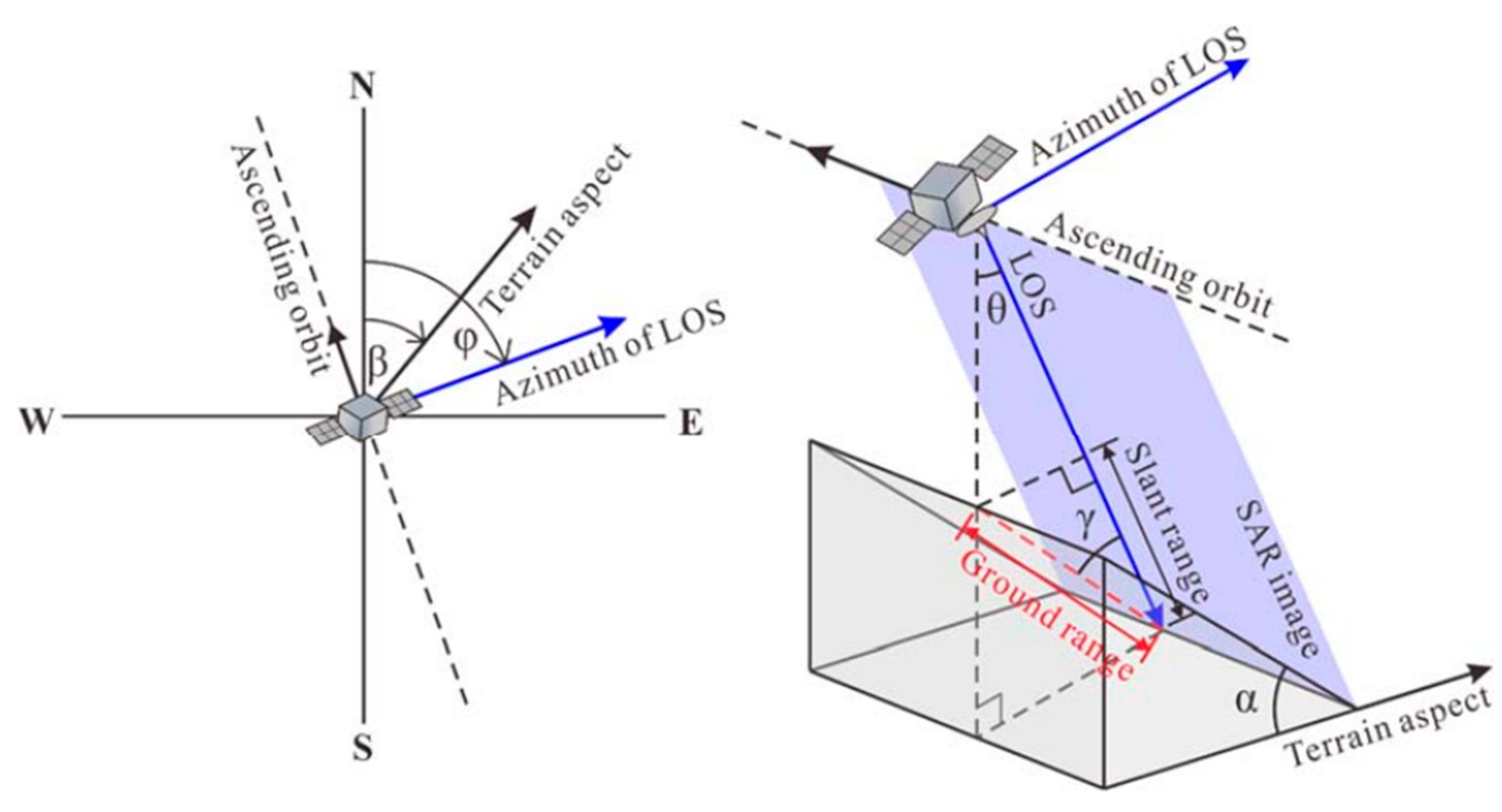
SAR displacement measurements are one-dimensional, capturing only the movement component along the LOS (Line Of Sight), which is tilted with respect to the vertical at an angle that varies depending on the satellite and the acquisition geometry. In flat terrains and slopes exposed to the north or south, two-dimensional analysis is possible using ascending and descending passes. However, the system exhibits limited sensitivity along the direction of the sensor orbital. Since the orbits of the main satellites (ERS, Sentinel, RADARSAT) are almost polar, any deformation occurring along the north-south direction results in minimal projection along the LOS. To address this limitation, a correction index C can be applied to each LOS measurement to compute the actual velocity component in the slope direction (V
SLOPE). The
C index accounts for satellite-dependent parameters, such as incidence angle θ, i.e., the inclination of the LOS with respect to the vertical, and track angle φ, i.e., the angle between the projection of the satellite trajectory on the horizontal plane and geographic north, as well as topographic parameters, including terrain slope α and orientation β [
20,
26] (
Figure 1).
The track angle and incidence angle are provided within the processed SAR images for each satellite, while slope and aspect values are derived from a DTM. The resolution of the DTM significantly influences the accuracy of the C index. High-resolution DTMs improve the representation of terrain profiles but introduce greater variability in slope and aspect values, impacting C index computation and subsequent V
SLOPE calculations. For balanced accuracy and computational efficiency, a cell resolution of at least 20 m is recommended, consistent with InSAR data resolution [
25]. The
C index represents the component of movement detectable by the SAR sensor, with a value ranging from -1 to 1.
The
C index is a function of the incidence and track angles and the characteristics of the slope and can be calculated as follows:
where S is the slope of the surface; A is the aspect of the surface with respect to the north; N, E, and H are direction cosines [
20]. This allows the calculation of V
SLOPE (mm/year), the projection of the LOS velocity (V
LOS) along the direction of maximum slope, using the following relationship [
27,
28]:
The relationship also allows for estimating whether the movement is toward or away from the satellite. Indeed, for values of C close to 1, the satellite accurately observes the movement, and V
SLOPE tends to V
LOS. For negative C values, the movement is recorded in the reverse direction relative to the LOS geometries. In this case, if the velocity components are consistent with the movement along the slope, V
SLOPE will have a sign opposite to V
LOS. For values of C close to zero, V
SLOPE tends toward infinity, significantly amplifying errors in the projection [
20]. Furthermore, it should be noted that positive V
LOS values can indicate either potential errors or real movements. When V
SLOPE shows a positive value, it may indicate that a landslide is moving upward rather than downward, an unlikely condition. Therefore, such cases should be assessed individually [
20].
The processing model in QGIS generates a percentage visibility map that illustrates proportion of the velocity V
LOS along the direction of maximum slope. The percentage of visibility is calculated using the formula:
This thematic map helps in quantifying the proportion of the terrain visible to the satellite, accounting for the radar acquisition angles. The visibility percentage serves as a critical metric for assessing the capability of the satellite to acquire accurate and comprehensive data. Additionally, the algorithm generates a visibility classification map that categorizes the terrain into five distinct classes based on visibility levels. This classification provides a detailed representation of areas with varying monitoring precision, highlighting regions where data acquisition is more effective.
The calculation of the
C index has been implemented in the
Geohazard plugin, input data and results are shown in
Table 1.
3.1. Validation of the Model
For validation purposes, the results generated by the model on a training dataset were compared with externally performed calculations. The DTM of the training dataset represents a high mountain area of 154x172 m
2 in Piemonte (Italy). The DTM has a cell size of 25 m to balance accuracy and computational efficiency. An Excel spreadsheet was created to facilitate this comparison, incorporating Equation 1 to derive the
C index. This approach enabled a direct comparison between the output of the algorithm and the externally calculated values. A validation process was carried out on nine cells, with three cells selected for each pair of angles. The input data for the
C index calculation included aspect, slope, incidence angle θ, and track angle φ, and the corresponding values were assigned to each cell being validated. The comparison of results confirmed the validity and accuracy of the model, as outlined in
Table 2.
4. Landslide – Shalstab
Shalstab is a physically-based model used to assess the triggering of shallow landslides due to infiltrated rainfall, following the method proposed by Montgomery & Dietrich (1994) [
21] and Dietrich and Montgomery (1998) [
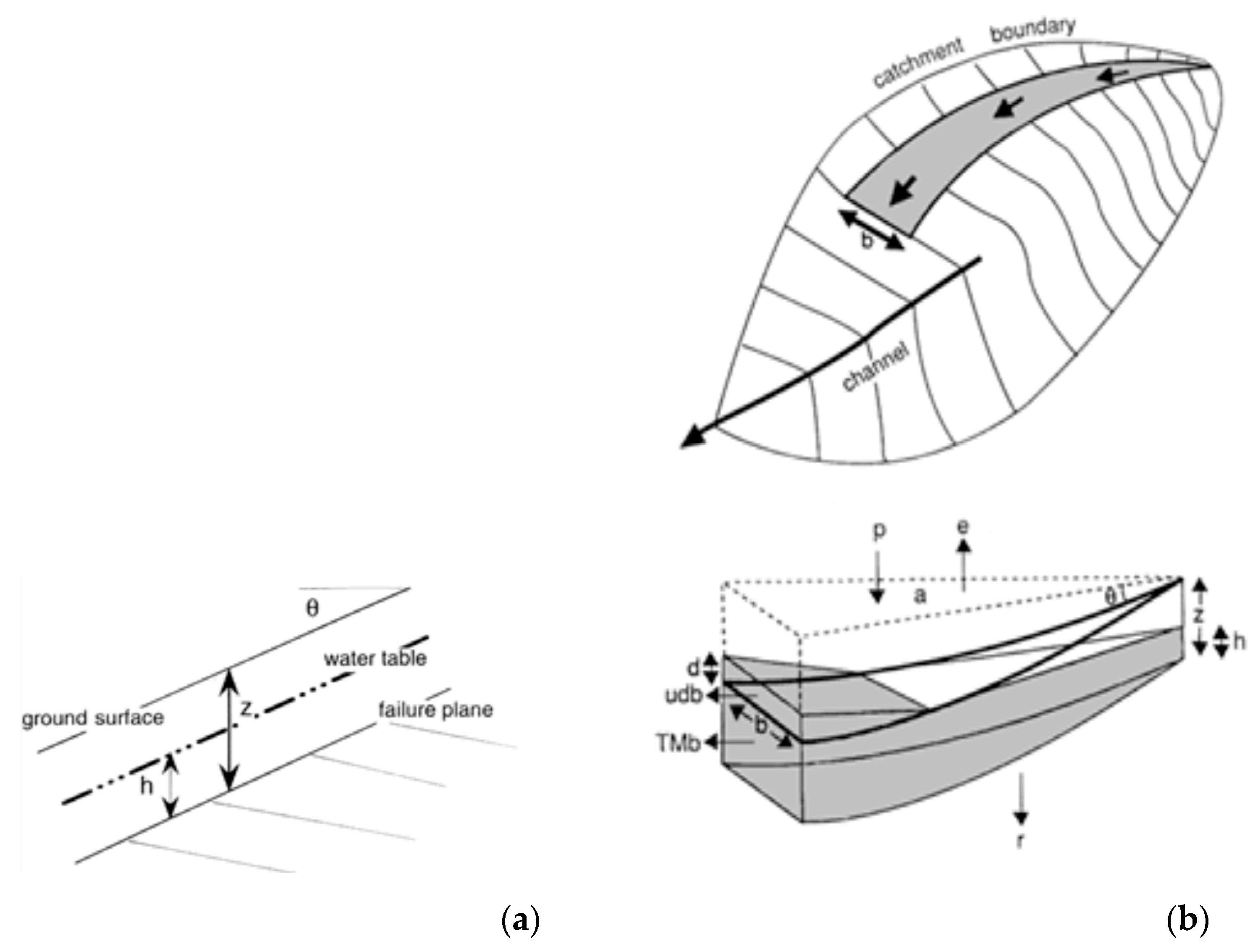
29]. The method (
Figure 2) enables the analysis of topographic, soil, and rainfall data to evaluate slope stability and solves the relevant equations using a gridded representation of the terrain, combining a limit equilibrium stability model for infinite slopes with a steady-state hydrological model. The main assumptions underlying the formulation are as follows [
30,
31]:
infinite slope;
planar failure surface, parallel to the slope, located at the interface between the shallow layer and the underlying layer of lower permeability;
Mohr-Coulomb shear strength criterion expressed in terms of effective stresses;
steady flow parallel to the slope;
absence of deep drainage and flow within the underlying substrate.
According to the Limit Equilibrium Method, the stability condition is determined by calculating the Factor of Safety (
Figure 2a and Equation 4):
where θ is the slope inclination, z is the landslide thickness, c’ and
’ are cohesion and friction angle respectively,
is soil unit weight, u is water pressure on the failure surface,
is water unit weight, and h is the water table level above the failure plane.
There are several approaches to consider the effects of rainfall and its infiltration into the soil. In
Shalstab, steady-state conditions are assumed, meaning there is no temporal variation in rainfall and soil saturation. The model is based on the observation that shallow landslides tend to occur in topographic hollows, where shallow subsurface flow convergence leads to increased soil saturation, pore pressure, and reduced shear strength, thus triggering potential failure. The hydrological component of the model is simplified by assuming that rainfall infiltrates the soil and is routed downslope, following the topographic gradient. This implies that the contributing area at any given point is defined by the specific catchment area derived from the surface topography (
Figure 2b).
For a detailed analytical discussion of the hydrological model employed in
Shalstab, reference can be made to [
29]. The following section outlines the hydrologic component of this model that, coupled with the stability component (Equations 4 and 5) leads to the implementation of the F
S equation (Equation 6):
The instability condition (F
S ≤ 1) for each cell in the domain is expressed by (Equation 7):
a is the contributing upslope area draining across the contour length b;
and Ks is the permeability coefficient of saturated soil;
and q is effective rainfall.
This condition is evaluated only for cells that do not meet the conditions of absolute stability and absolute instability, given by:
The condition of absolute stability identifies cells classified as stable even when the soil is fully saturated. The condition of absolute instability indicates cells that are unstable even in the absence of infiltration.
Furthermore, by imposing the limit equilibrium condition (F
S = 1) and solving Equation 7 with respect to q, the critical infiltration q
cr threshold can be determined (Equation 10):
If the information on the presence of roots in the shallow soil layers is available, their resistance contribution can be incorporated by increasing the soil cohesion, which will then be composed by the sum of the contribution of soil csoil and roots croot.
Based on the aforementioned method, the
Shalstab algorithm provides the spatial distribution of the absolute stable and absolute unstable cells, as well as the critical effective (infiltrated) rainfall that leads each cell to a F
S of 1. The required input data are listed in
Table 3. Although most parameters vary spatially across the slope, to assist the user in preparing a quick analysis, the
Geohazard plugin includes an additional tool called
Shalstab input raster creator, which allows for the generation of constant-value input raster files from the DTM.
The results of the analysis are given as 4 raster maps, showing: 1) absolute stable zones; 2) absolute unstable zones; 3) distribution of critical infiltrated rainfall q
cr (mm/day); 4) susceptibility classes. In the q
cr map, absolute stable cells assume no data values and absolute unstable cells assume q
cr = 0. The susceptibility raster map is a reclassification of q
cr in 7 classes (
Table 4) as suggested by Dietrich and Montgomery (1998) [
29]. This classification provides the value of q
cr/T in logarithmic form. This ratio reflects the magnitude of the water infiltration, represented by q, concerning the ability of the surface to move the water downslope, i.e., the transmissivity (T). The larger the value of q relative to T, the more likely the ground is to become saturated. This is a useful representation for identifying areas of the study domain with different behaviour and it can be interpreted as a susceptibility map since it spatially classifies the distribution of instability conditions. It can be converted into a hazard map if an infiltration model is applied, to compute a critical triggering gross rainfall P
cr from q
cr. Given P
cr, the probability of occurrence of the related meteorological event can be made explicit as a return period and the time dimension of hazard is achieved [
32].
4.1. Validation of the Model
For the validation of the model, it was applied to the 10 m resolution DTM of the Dego area, south Piemonte (Italian National Geological Mapping Project, sheet 211), which was used to create the landslide hazard map for the Carg Project [
33]. In the Carg Project, absolute hazard was defined, including the temporal aspect through the return period of critical rainfall and the assessment of the destructive potential of the phenomenon (intensity). To validate the model, input data derived from the Carg Project were used (
Table 5), and the results obtained in terms of absolute stable, absolute unstable cells, and distribution of q
cr were compared.
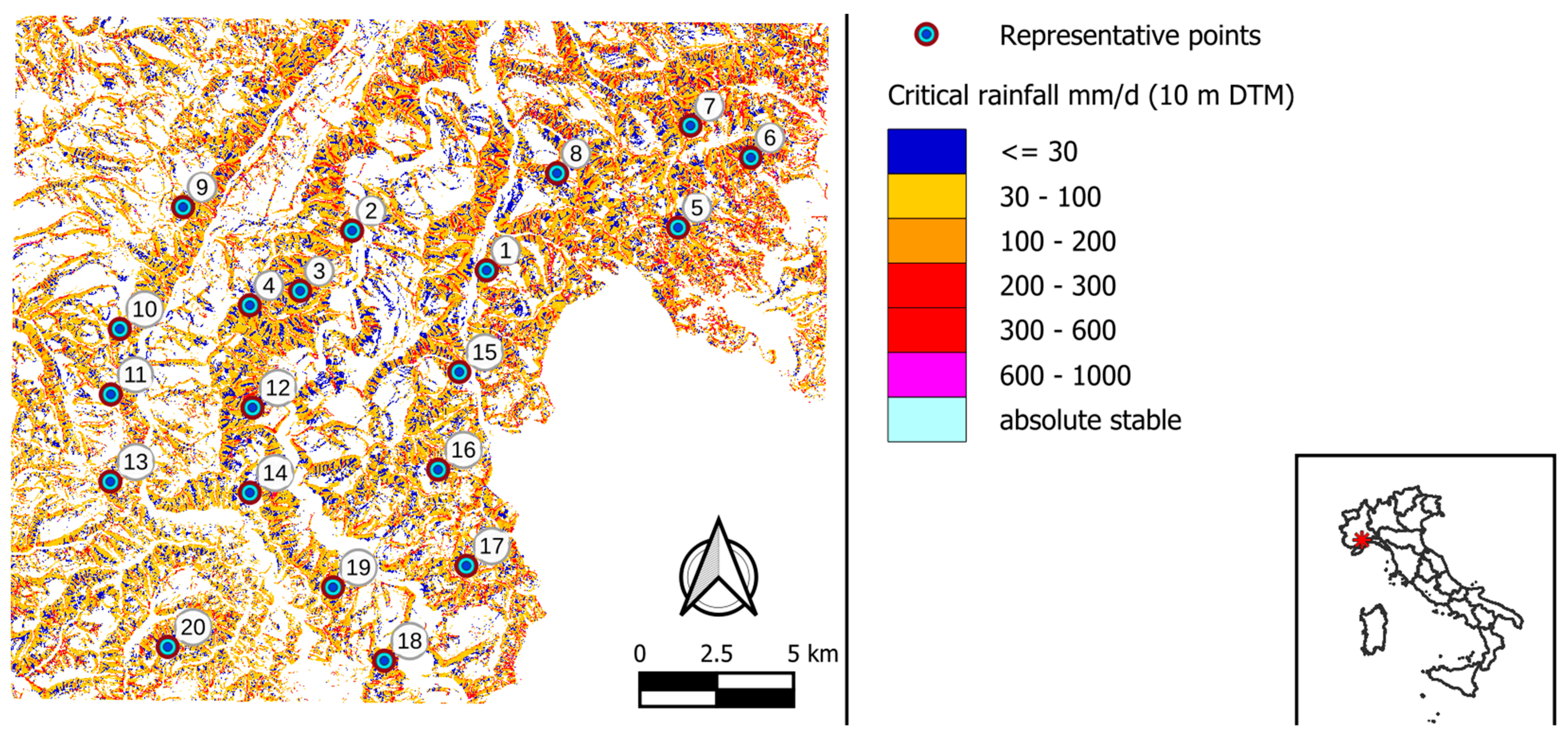
In
Figure 3, the resulting critical rainfall map (q
cr) is shown after applying the Shalstab model to the Dego area. Twenty representative cells in different areas were considered for comparison (
Table 6): the values of critical infiltration vary with negligible differences, due to the use of different hydrology calculation algorithms. However, this comparison highlights the accuracy of the obtained results, and the validation can be considered successful.
In addition, to evaluate the influence of DTM cell size on the analysis results, a calculation was repeated on the same area using the 5 m DTM provided by Regione Piemonte. Again, the parameters listed in
Table 5 were used. In
Table 7 the critical rainfall q
cr is reported for the 20 representative points referred to in the 10 m and 5 m DTM analyses. The susceptibility classes are also reported for comparison. The results show that the difference in q
cr calculation can be not negligible. This is probably due to the fact that DTM resolution affects both the mechanical (Fs) and the hydrological component of the model, resulting in different inclinations of the slope in each cell and thus in different catchment area calculations. This aspect of the problem, that affects the susceptibility classification of the area, will be further analysed in the future.
5. Rockfall – Droka
The Droka model is devoted to the simplified analysis of rockfall runout from diffuse source points across a slope. The analysis is based on the concept of energy line, the line connecting a rockfall source point to the farthest stopping point of a block detached from that source. The energy line is inclined at an angle p with respect to the horizontal plane (i.e., the energy angle), which can be interpreted as a global block-slope friction angle. This angle is representative of all the dissipative phenomena occurring throughout the motion phases of the block along the slope. The concept of energy line is implemented in the Geohazard plugin through two independent yet complementary algorithms: Droka_Basic and Droka_Flow. Both simulations provide results in the form of point vectors, distributed across the invasion zone. For each point, the following information is provided: minimum, maximum, and mean block velocity [m/s]; minimum, maximum, and mean kinetic energy [kJ]; and the number of simulations that affected a specific point (frequency).
The two models use different methods to identify the areas involved in the phenomenon and can be used independently or combined to obtain complementary information. A detailed description of the algorithms is provided below along with a discussion of their potential and limitations through practical application examples.
5.1. Rockall - Droka_Basic
Droka_Basic module is based on the Cone method [
10,
18,
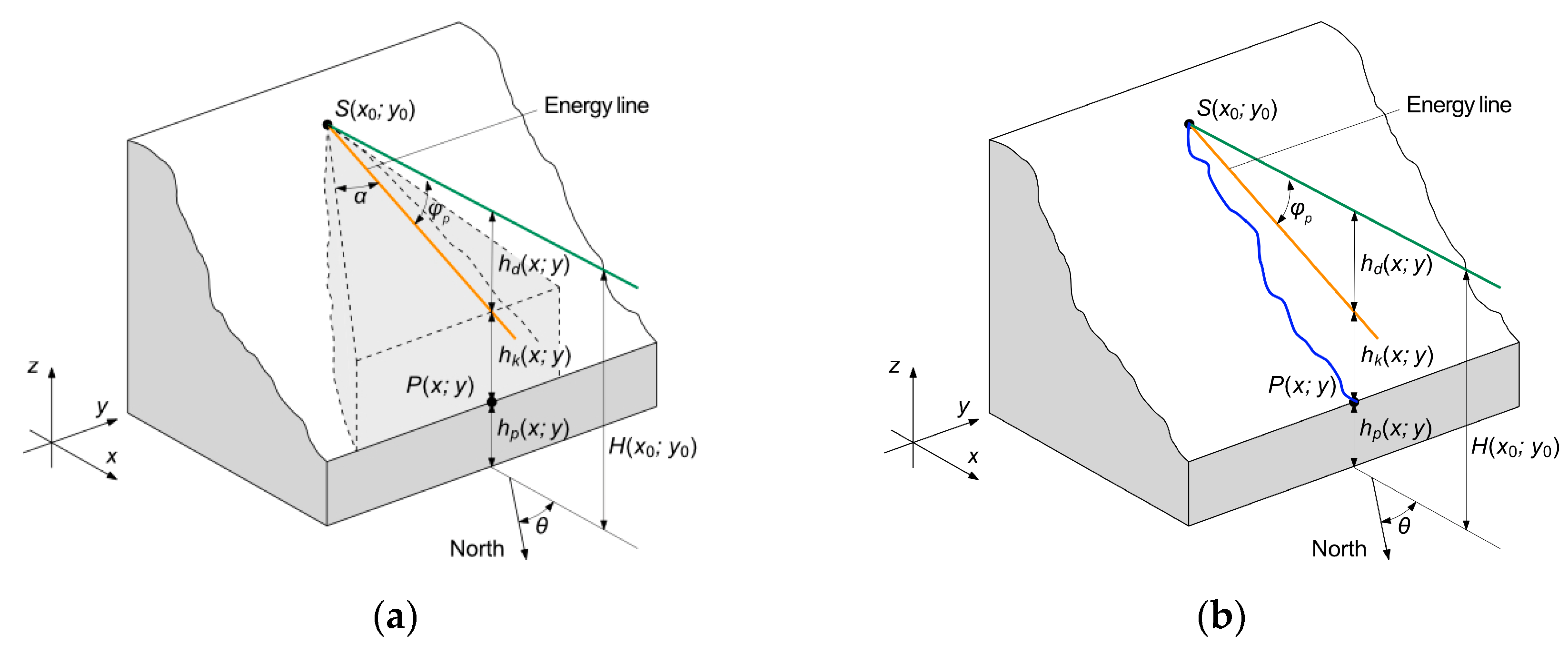
22], which enables the definition of the area affected by rockfall events on a slope. This is achieved through a cone representing the envelope of all possible rockfall paths. The apex of the cone is located at the source point and its geometry is defined by three angles (
Figure 4a): the dip direction angle θ of the slope at the source point defines the orientation of the cone; the energy angle
p outlines its vertical extension and the lateral spreading angle α delineates the extension of the cone in the horizontal plane. The intersection of the cone with the surface of the slope defines the rockfall-affected area, where each point within this area may potentially be reached by a rockfall path originating from the source. When multiple source points are considered, the module can delineate zones subjected to rockfalls through the overlapping of simulated cones. This approach enables the creation of a frequency map, where areas with higher frequencies are the most prone to be reached by fallen blocks, identifying them as the most susceptible to this type of danger. Using the concept of the energy line, the module enables the calculation of the velocity and kinetic energy of the block at any position within the affected area [
18]:
where g is gravity acceleration, (x
0,y
0) are the source point coordinates, H(x
0,y
0) is the elevation of the source point, h(x,y) is the elevation of the topographic surface in the point (x,y),
p is the energy angle.
Therefore, the kinetic energy E can be estimated at any position given the block mass m [
18]:
The Cone Method in the
Droka_Basic module is implemented by constructing a triangle with its apex at each source point, characterized by specified input parameters. A point layer is then generated, containing one point for each DTM cell covered by the triangle. For each point, the height difference ΔH between the ground and the energy line is computed (ΔH=h
k(x,y),
Figure 4a). Points showing a positive ΔH value are identified as part of the invasion area. Starting from ΔH, block velocity and kinetic energy are computed for each point according to Equations 11 and 12.
The input data required by the
Droka_Basic module are described in
Table 8. The attributes of source points are obtained from the DTM while the cone parameters are constant across all source points and are specific to each case study. Calibrating these parameters is essential to achieve reliable and conservative results. It should be based on information from past events in the area, rockfall inventories, territorial databases, and quick field observations of the slope. The output is a vector layer of points located at the center of the DTM cells within the affected area, containing the data listed in
Table 8.
5.2. Rockfall – Droka_Flow
The Droka_Flow module employs a hydrological approach to simulate potential rockfall paths by tracing the line of maximum slope for each source point. The path terminates when the inclination of the line passing through the source point is lower than the inclination of the energy line, defined by the user.
Each analysis includes five simulations from each source point. These simulations adjust DTM elevation using a Monte Carlo approach within a user-defined standard deviation around the original DTM elevation values, assuming a simplified normal distribution of elevation for each cell. The mean corresponds to the original DTM height, while the user-defined standard deviation is constant across cells. This approach provides a simplified representation of the variability in rockfall trajectories due to factors like ground impact, bouncing, and obstacles (e.g., rocks, trees, or structures).
The
Droka_Flow module relies on the GRASS GIS function
r.drain to calculate five paths from each source point. As with
Droka_Basic, the analysis result is a vector point layer is then generated, containing one point for each DTM cell covered by the simulated paths. For each point, the height difference ΔH between the energy line and the ground is calculated, leading to block velocity and kinetic energy calculations when ΔH is positive (Equations 11 and 12;
Figure 4b). The paths are then merged for the statistical analysis of block velocity and kinetic energies.
The input data required by the
Droka_Flow module are described in
Table 9. Again, source points are obtained from the DTM while the energy angle and the standard deviation of the distribution of cells elevation are specific to each case study. In particular, the standard deviation should be related to the DTM size, as discussed in
Section 6. The output is a vector layer with point attributes similar to those described in
Droka_Basic and listed in
Table 8. Frequency data is omitted here due to the limited number of paths per source point, so energy count and percent fields are not included.
5.3. Validation of the Modules
To validate the results produced by the algorithms implemented in
Droka_Basic and
Droka_Flow modules, an initial set of analyses was carried out on a synthetic slope DTM with 5 m cell size. The slope was generated by joining two planar surfaces: a runout plane inclined at 60° to the horizontal and a nearly horizontal plane with an inclination of approximately 2°. A single rockfall source point was located at an elevation of approximately 500 m, with a mass of 2600 kg and a volume of 1 m
3. Parametric analyses were performed on this synthetic slope to assess the influence of key parameters on the results, using both
Droka_Basic and
Droka_Flow. The best parameters fit for both
Droka modules was found to be lateral spreading angle α equal to 10°, and standard deviation equal to 0.1 m. The results are consistent for the modules, as reported in
Figure 5, and align with the simplified analytical model in the calculation of block velocity and kinetic energy, following Equations 11 and 12.
However, for natural slopes, where both aspect and inclination vary widely, rockfall trajectories may spread much more. In addition, natural slopes feature niches, incisions, or debris accumulations due to erosion and instability phenomena over time, which significantly influence the rockfall paths. Therefore, it is suggested to calibrate the parameters for susceptibility analyses to the specific site conditions. A proper calibration can be achieved through the back analysis of actual events, using data gathered from in situ observations, as described in
Section 6.
6. Application of Rockfall – Droka Modules: Bobbio Pellice Case Study
This section presents an example of the application of the Rockfall - Droka modules for a preliminary assessment of rockfall susceptibility and relative spatial hazard, illustrating the recommended procedure and discussing the results. The example focuses on a steep slope near the village of Bobbio Pellice, Piemonte (Western Alps), where recurrent rockfall events threaten a cluster of alpine buildings. On 24 June 2024, a large rockfall event destroyed one of these buildings, creating high-risk conditions.
6.1. Parameter Calibration
The Bobbio Pellice rockfall event involved a slope sector impacted by similar events in the past and was triggered by intense meteorological conditions. Observations from the survey conducted by GeoAlpi Consulting (2024) [
34] include the following:
the detachment occurred at approximately 1,940 m a.s.l;
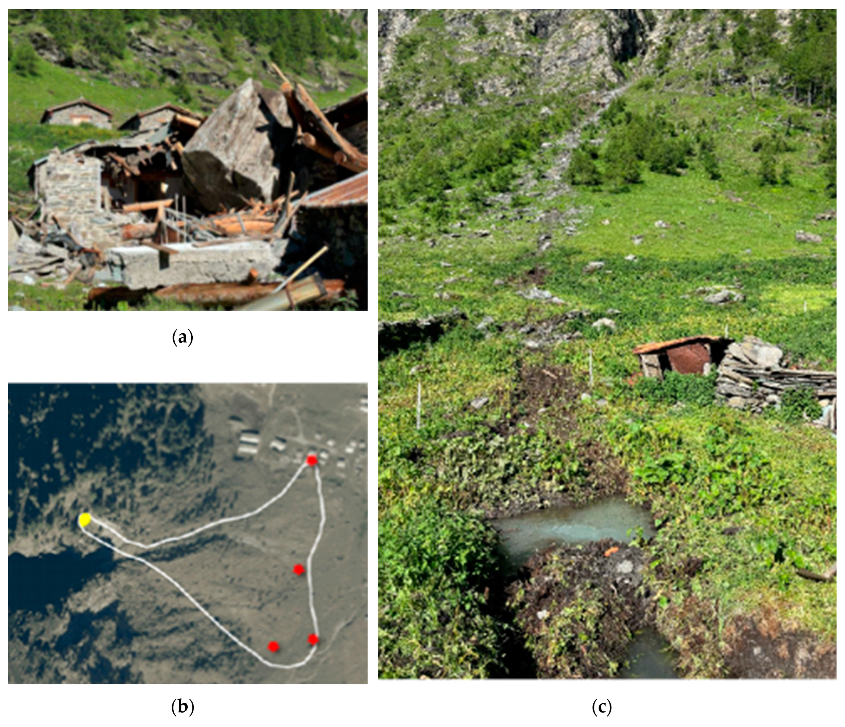
a block of approximately 30 m3 struck and destroyed a building located at about 1,750 m a.s.l., with visible traces along its trajectory (Figures 6a,c);
this path was influenced by other blocks and debris on the slope, displaced during all the collapses;
additional smaller blocks of approximately 1-2 m
3 reached the bottom of the valley, with clearly defined trajectories. The stopping position of some of these blocks is shown in
Figure 6b.
Based on the available information a back-analysis was performed; three source points were selected within the steepest area of the involved zone (
Figure 6b). A block with a volume of 30 m
3, mass of 78,000 kg and unit weight of 2600 kN/m
3 was used to estimate kinetic energy. The 5 m DTM provided by Regione Piemonte (2010) was employed for an initial set of analyses to calibrate parameters and compare the results from
Droka_Basic and
Droka_Flow.
For
Droka_Basic, the optimal results in terms of invasion area were achieved with a lateral spreading angle α of 22° and an energy angle φ
p of 37°, as shown in
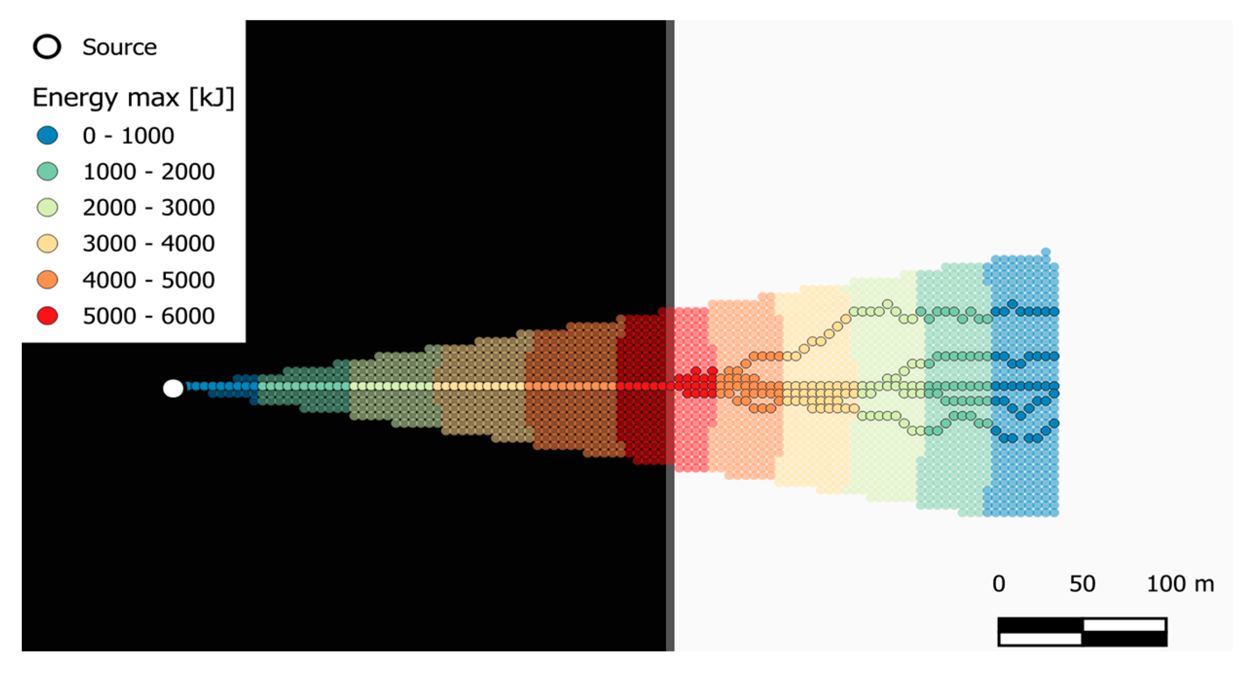
Figure 7, where the distribution of block kinetic energy within the invasion area is also included. The computed kinetic energy at the impact point with the building is approximately 5,000 kJ, consistent with the total destruction of the building.
To calibrate the
Droka_Flow model, the influence of the assumed standard deviation was analyzed in this study through a parametric analysis, with standard deviation values ranging from 0.1m to 5m (2% to 100% of DTM cell size). Each simulation was repeated 5 times to generate about 20 paths (
Figure 8). The results suggest that the most conservative simulations occur with standard deviations of 0.5 m and 1 m, corresponding to 10% and 20% of the 5 m DTM cell size, respectively. In these cases, at least one trajectory reaches the affected building, with kinetic energy around 5,000 kJ, consistent with the results from
Droka_Basic. As shown in
Figure 8, the simulated paths do not encompass the entire invasion area (in white), as only trajectories in the direction of maximum slope are simulated by the
r.drain function. Nonetheless, this analysis demonstrates that the location of the building is the most prone to being impacted by a block detached from the source area, indicating it as the most critical area. The combination of
Droka_Flow and
Droka_Basic provides dual insights: first, it identifies the entire area potentially impacted by the rockfall, accounting for all possible trajectories, including the less probable ones; second, it highlights the most critical paths within this area.
The back-analyses with
Droka_Basic and
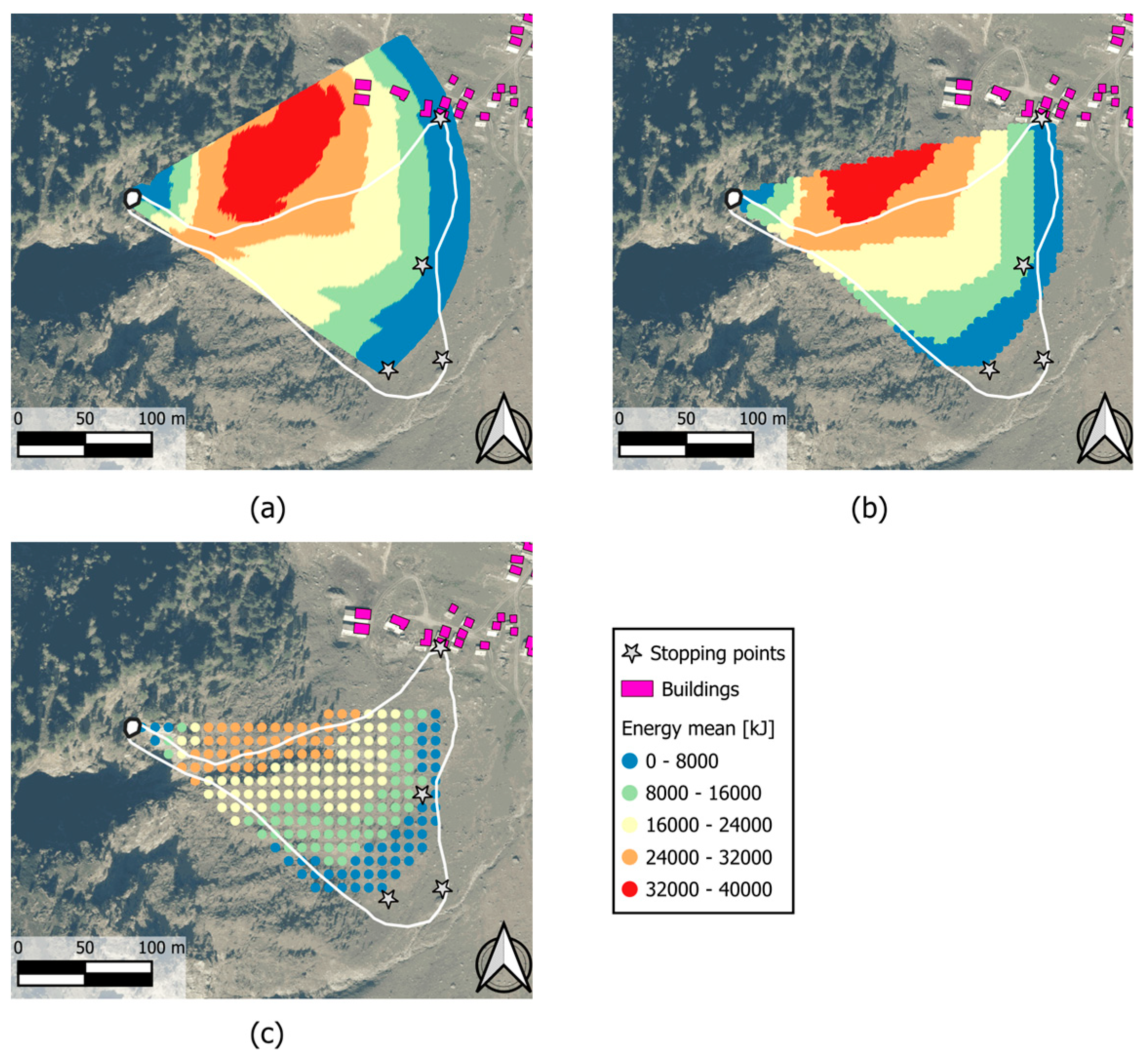
Droka_Flow modules were repeated with 1 m, 5 m and 10 m DTM resolutions for evaluating the influence of DTM resolution on the results.
Figure 9 shows the results of
Droka_Basic for the case with φ
p = 37° and α = 22°. It is worth noting that changes in DTM discretization slightly affect the orientation of source points. Specifically, the 1 m DTM results in greater variability in dip direction at source points compared to the 5 m and 10 m DTMs, leading to a wider invasion area. Despite this variability, a lateral spreading angle α of 22° remains the best calibration to cover the invasion area conservatively. In contrast, with the 10 m DTM, a conservative outcome requires increasing the α value. The optimal φ
p value for delineating the rockfall-affected area (37°) remains consistent across DTMs, suggesting it is a characteristic parameter of the phenomenon, dependent on the slope geometry and block properties rather than on DTM resolution.
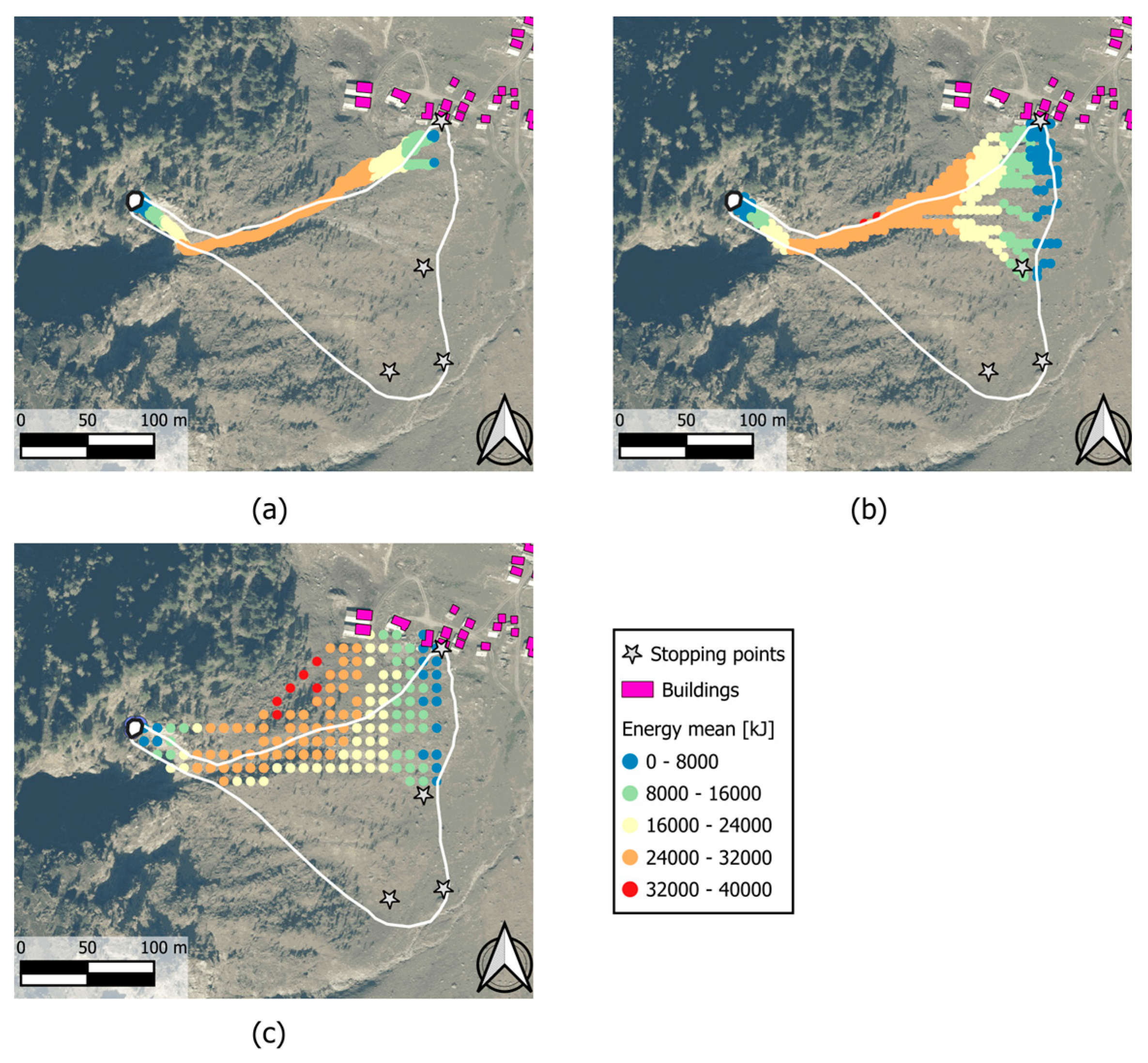
Figure 10 presents the results of
Droka_Flow for the case with φ
p = 37° and a standard deviation of 10% of the DTM size (i.e., 0.1, 0.5, and 1 m for DTM sizes of 1, 5, and 10 m, respectively), which yielded the most conservative results. This comparison shows that the 1 m DTM results in a very limited trajectory spread around the maximum slope path (this result is obtained regardless of the chosen standard deviation). The widest trajectory spread occurs with the 10 m DTM; however, many trajectories fall outside the designated rockfall invasion zone (shown in white in
Figure 10). The analysis that better simulates the actual invasion area seems to be with the 5 m DTM, for both
Rockall - Droka modules.
These observations suggest that effective parameter calibration for susceptibility and hazard analysis can be achieved through back-analysis conducted within the same geomorphological context and using the same DTM resolution, ensuring consistent results. As discussed, Droka_Basic and Droka_Flow modules complement each other, with their comparison highlighting both the most significant trajectories and the full invasion area. This combined approach offers valuable insights for defining rockfall susceptibility.
6.2. Susceptibility and Relative (Spatial) Hazard Analysis
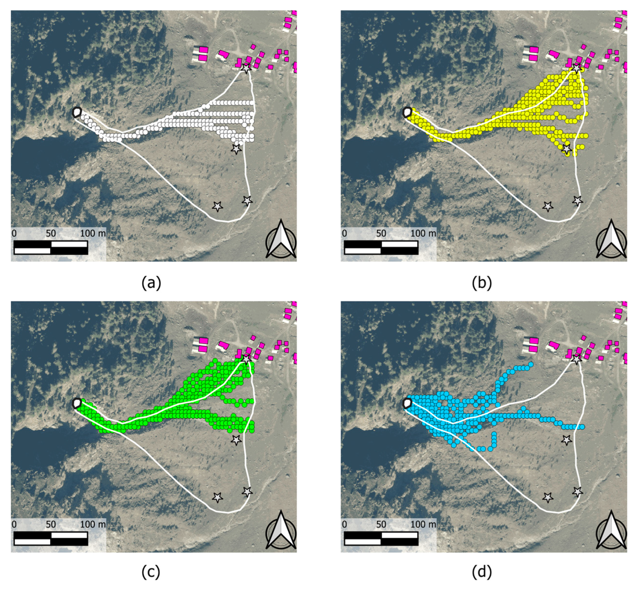
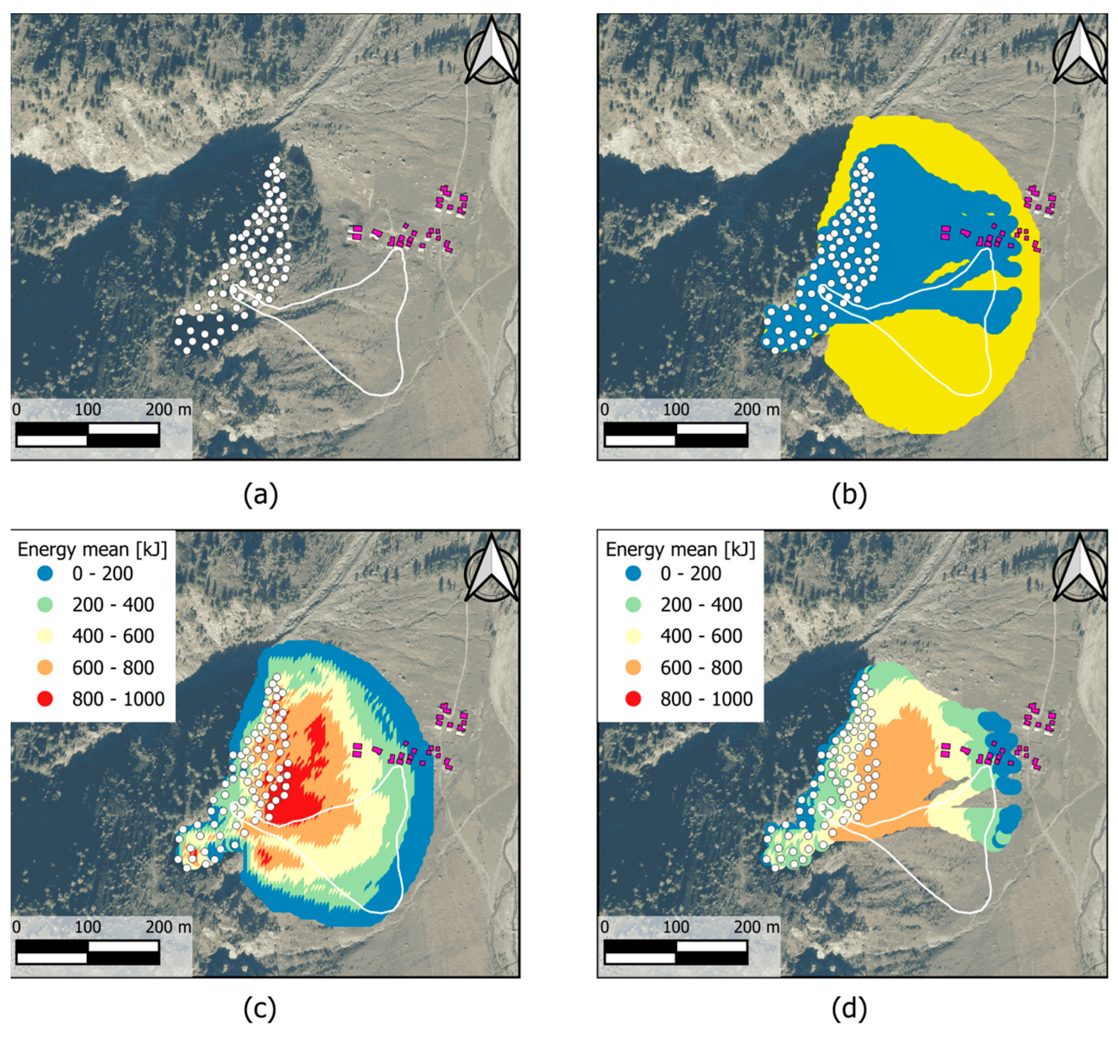
To exemplify the suggested procedure for susceptibility analysis, this study was extended to the slope surrounding the area where the buildings are located. Since no information was available to quickly identify the possible source areas, all DTM cells with an inclination greater than a specific threshold were selected on the slope above the buildings. Following [
35], the resulting threshold is 49° for a 5 m DTM. A total of 80 source points was randomly selected within cells exceeding this threshold, covering a slope sector approximately 200 m in length, as shown in
Figure 11a. Finally, a block with a volume of 1m
3 was used to estimate the kinetic energy.
Figure 11b compares the results of the analyses conducted with
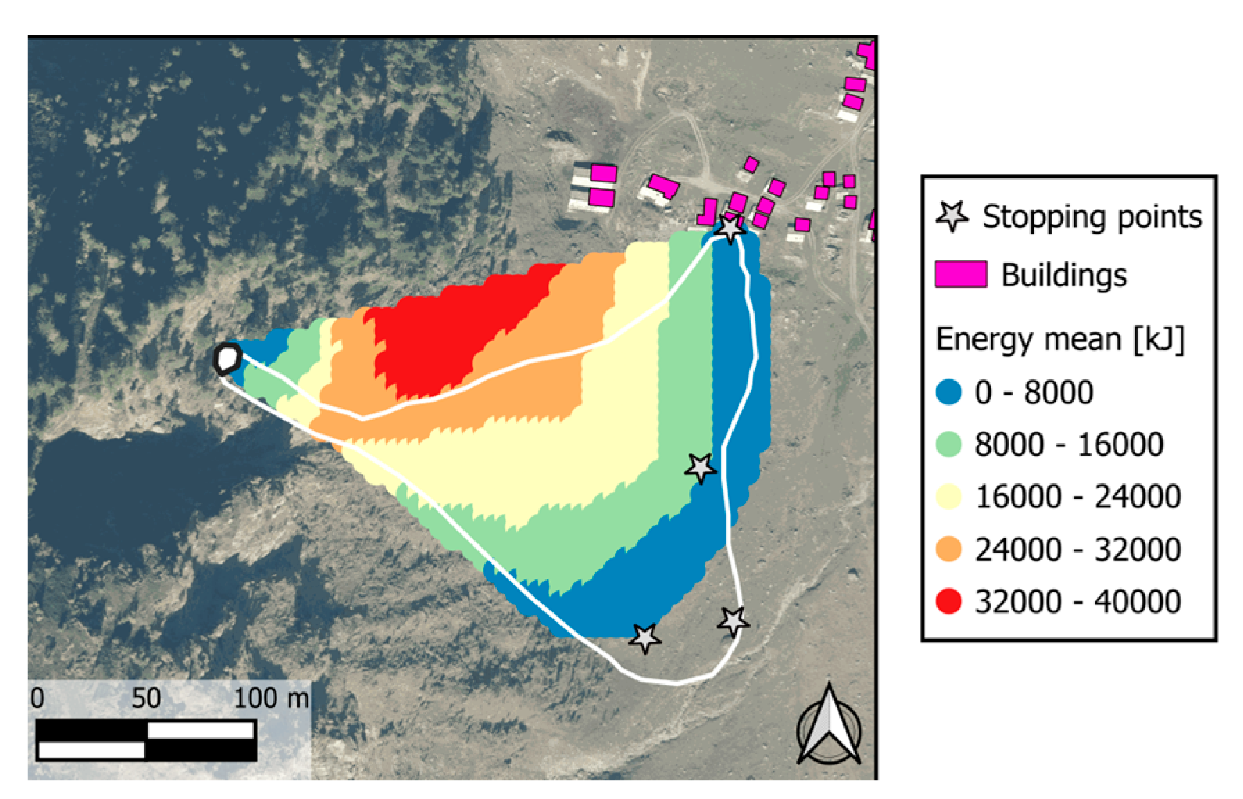
Rockfall - Droka modules in terms of runout area, while Figures 11c and 11d show the mean kinetic energy obtained by the two modules. To assess rockfall susceptibility, the
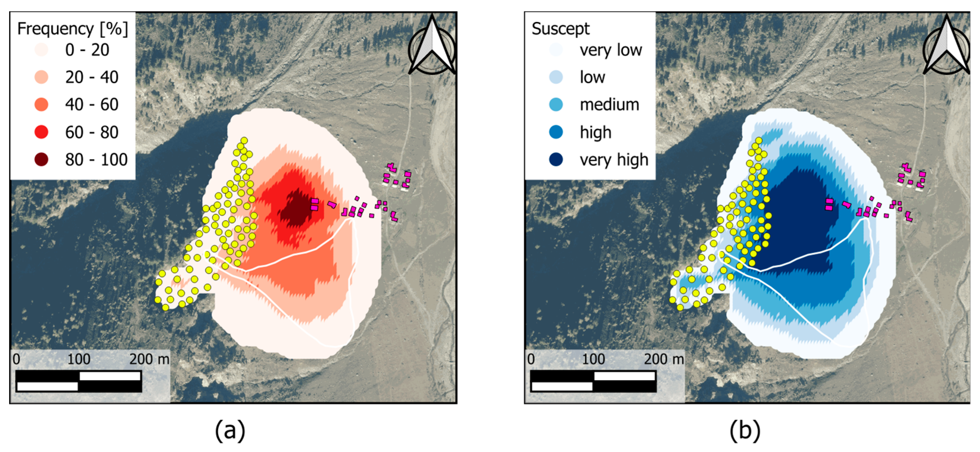
Droka_Basic spatial frequency results, defined as the number of overlapping cones out of the total source points (
Figure 12a), were multiplied by the mean kinetic energy values (
Figure 11c) at each point. The final output, shown in
Figure 12b, highlights the most critical zones by combining both spatial frequency and phenomenon intensity and can be interpreted as a relative (spatial) hazard.
The comparison between the results from
Droka_Basic and
Droka_Flow again confirms the consistency of the two algorithms.
Droka_Basic is more conservative regarding total invasion area (
Figure 11b) and mean kinetic energy (Figures 11c and 11d), as the area covered by rockfall paths simulated by
Droka_Flow (
Figure 11b) is concentrated in the northern part of the invasion zone and shows lower mean kinetic energy values in the central region. However,
Droka_Basic indicates the highest frequency in this central zone (
Figure 12a), suggesting that blocks from multiple source points can reach it. Differences in the mean kinetic energy calculated by the two algorithms arise from statistical comparisons based on different sample populations, although the maximum kinetic energy values computed are identical across the entire area. Regarding slope susceptibility and relative (spatial) hazard, the results from both algorithms are again consistent, highlighting the critical situation for certain buildings. This finding underscores the need for a more detailed analysis to accurately assess the risk to these structures and to establish appropriate mitigation measures.
7. Conclusions
In this paper, the Geohazard plugin is presented. The plugin is developed as an open-source tool within the QGIS environment and it offers a useful and user-friendly framework for assessing geohazards, related to landslides and rockfalls. By integrating several algorithms, it addresses challenges associated with complex geomorphological conditions, providing actionable insights for hazard management and mitigation at medium-small scale.
The
Groundmotion – C Index module [
20] demonstrated its reliability during validation on a training dataset with a 25 m cell size DTM, where its results closely matched external calculations. The analysis improved the interpretation of InSAR data for slow-moving landslides.
The
Landslide - Shalstab module effectively evaluated the susceptibility to shallow landslides by calculating the critical rainfall infiltration required to trigger instability. Validation on the Dego area (located in the hilly Langhe region, north-western Italy), using a 10 m cell size DTM and consistent input parameters confirmed the ability of the model to delineate areas prone to shallow landslides, with results aligning well with hazard maps developed in previous studies [
30]. The critical rainfall map (q
cr) and derived susceptibility classifications provided valuable insights into the spatial distribution of instability conditions, which can be further refined into hazard assessments through rainfall and infiltration modeling.
The
Rockfall - Droka_Basic and
Droka_Flow modules for rockfall analysis were applied to the Bobbio Pellice case study, an area in the Italian Western Alps [
34], to assess rockfall affected zones and relative (spatial) hazard. Parameter calibration based on a well-documented rockfall event in the Bobbio Pellice area enabled accurate delineation of invasion zones and identification of critical trajectories.
Droka_Basic captured the overall invasion zone using energy and lateral spreading angles, while
Droka_Flow simulated individual trajectories, both providing preliminary estimates of block velocities and kinetic energy. Results showed that the destroyed building in the area was located in a critical zone, with estimated block kinetic energy exceeding 5,000 kJ.
These findings illustrate the reliability of the Geohazard plugin in addressing diverse geohazard challenges. The combination of algorithms provides a toolkit for geohazard assessment, enhancing the understanding of slope instability phenomena and supporting decision-makers in planning and implementing effective risk mitigation strategies.
In a time of increasing hydrogeological instability driven by climate change, the need for effective
prevention strategies has become a critical priority for protecting both people and infrastructure from hazardous events. Prevention, as a key aspect of climate change adaptation, requires proactive measures to reduce the impacts of geohazards. This work aims to support and enhance
prevention strategies, which are essential in the context of vulnerable territories such as Italy, where almost 94% of the Italian municipalities are at risk of landslides, floods, and coastal erosion, with over 8 million people living in high-hazard areas [
36].
Author Contributions
Conceptualization, M.C., A.F. and S.C.; methodology, M.C., A.F., G.T., S.C. and R.P.; software, A.F. and C.F.; validation, M.C., A.F., C.F., S.C.; resources, M.C. and R.P.; data curation, A.F., S.C. and R.P.; writing—original draft preparation, M.C., A.F., S.C. and G.T.; writing—review and editing, G.T.; supervision, M.C. and R.P. All authors have read and agreed to the published version of the manuscript.
Funding
This research received no external funding.
Data Availability Statement
Conflicts of Interest
The authors declare no conflicts of interest.
References
- Seneviratne, S.I. Nicholls, D. Easterling, C.M. Goodess, S. Kanae, J. Kossin, Y. Luo, J. Marengo, K. McInnes, M. Rahimi, M. Reichstein, A. Sorteberg, C. Vera, and X. Zhang, (2012). Changes in climate extremes and their impacts on the natural physical environment. In: Managing the Risks of Extreme Events and Disasters to Advance Climate Change Adaptation [Field, C.B., V. Barros, T.F. Stocker, D. Qin, D.J. Dokken, K.L. Ebi, M.D. Mastrandrea, K.J. Mach, G.-K. Plattner, S.K. Allen, M. Tignor, and P.M. Midgley (eds.)]. A Special Report of Working Groups I and II of the Intergovernmental Panel on Climate Change (IPCC). Cambridge University Press, Cambridge, UK, and New York, NY, USA, pp. 109-230.
- Crozier, M.J. Deciphering the effect of climate change on landslide activity: A review. Geomorphology 2010, 124, 260–267. [Google Scholar] [CrossRef]
- Picarelli, L.; Lacasse, S.; Ho, K.K. 2021. The impact of climate change on landslide hazard and risk. Understanding and Reducing Landslide Disaster Risk: Volume 1 Sendai Landslide Partnerships and Kyoto Landslide Commitment 5th, 131-141.
- Fell, R.; Corominas, J.; Bonnard, C.; Cascini, L.; Leroi, E.; Savage, W.Z. Guidelines for landslide susceptibility, hazard and risk zoning for land-use planning. Eng. Geol. 2008, 102, 99–111. [Google Scholar] [CrossRef]
- Van Westen, C.J.; Castellanos, E.; Kuriakose, S.L. Spatial data for landslide susceptibility, hazard, and vulnerability assessment: An overview. Eng. Geol. 2008, 102, 112–131. [Google Scholar] [CrossRef]
- Ferlisi, S.; Gullà, G.; Nicodemo, G.; Peduto, D. A multi-scale methodological approach for slow-moving landslide risk mitigation in urban areas, southern Italy. Euro-Mediterranean J. Environ. Integr. 2019, 4, 1–15. [Google Scholar] [CrossRef]
- Varnes, D.J. Landslide types and processes. Landslides Eng. Pract. 1958, 24, 20–47. [Google Scholar]
- Hungr, O. Dynamics of rapid landslides. Prog. Landslide Sci. 2007, 47–57. [Google Scholar]
- Lacasse, S.; Nadim, F. Landslide Risk Assessment and Mitigation Strategy. In Landslides–Disaster Risk Reduction; Springer: Berlin/Heidelberg, Germany, 2009; pp. 31–61. [Google Scholar]
- Scavia, C.; Barbero, M.; Castelli, M.; Marchelli, M.; Peila, D.; Torsello, G.; Vallero, G. Evaluating Rockfall Risk: Some Critical Aspects. Geosciences 2020, 10, 98. [Google Scholar] [CrossRef]
- Van Westen, C.J. Remote Sensing and GIS for Natural Hazards Assessment and Disaster Risk Management. In Treatise on geomorphology; Academic Press: Cambridge, MA, USA, 2013; pp. 259–298. [Google Scholar] [CrossRef]
- Filipello, A.; Giuliani, A.; Mandrone, G. Rock Slopes Failure Susceptibility Analysis: From Remote Sensing Measurements to Geographic Information System Raster Modules. Am. J. Environ. Sci. 2010, 6, 489–494. [Google Scholar]
- Poursanidis, D.; Chrysoulakis, N. Remote Sensing, natural hazards and the contribution of ESA Sentinels missions. Remote. Sens. Appl. Soc. Environ. 2017, 6, 25–38. [Google Scholar] [CrossRef]
- Noviello, C.; Verde, S.; Zamparelli, V.; Fornaro, G.; Pauciullo, A.; Reale, D.; Nicodemo, G.; Ferlisi, S.; Gulla, G.; Peduto, D. Monitoring Buildings at Landslide Risk With SAR: A Methodology Based on the Use of Multipass Interferometric Data. IEEE Geosci. Remote. Sens. Mag. 2020, 8, 91–119. [Google Scholar] [CrossRef]
- Meissl, G. Modelling the runout distances of rockfall using a geographic information system. Z. Für Geomorphologie. Suppl. 2001, 125, 129–137. [Google Scholar]
- Wichmann, V. The Gravitational Process Path (GPP) model (v1. 0)—a GIS-based simulation framework for gravitational processes. Geosci. Model Dev. 2017, 10, 3309–3327. [Google Scholar] [CrossRef]
- Carrara, A. , Cardinali M., Detti R., Guzzetti F., Pasqui V. & Reichenbach P. (1990). Geographical Information Systems and Multivariate Model in Landslide Hazard Evaluation, In Alps 90, A.cancelli (Ed.) 6th Int. Conf. And Field. Workshop on Landslides, Milano, pp. 17 - 28.
- Castelli, M.; Torsello, G.; Vallero, G. Preliminary Modeling of Rockfall Runout: Definition of the Input Parameters for the QGIS Plugin QPROTO. Geosciences 2021, 11, 88. [Google Scholar] [CrossRef]
- GEOHAZARD PLUGIN Available online: https://github.
- Notti, D.; Herrera, G.; Bianchini, S.; Meisina, C.; García-Davalillo, J.C.; Zucca, F. A methodology for improving landslide PSI data analysis. Int. J. Remote. Sens. 2014, 35, 2186–2214. [Google Scholar] [CrossRef]
- Montgomery, D.R.; Dietrich, W.E. A physically based model for the topographic control on shallow landsliding. Water Resour. Res. 1994, 30, 1153–1171. [Google Scholar] [CrossRef]
- Jaboyedoff, M.; Labiouse, V. Technical Note: Preliminary estimation of rockfall runout zones. Nat. Hazards Earth Syst. Sci. 2011, 11, 819–828. [Google Scholar] [CrossRef]
- Copernicus - European Ground Motion Service. Available online: https://egms.land.copernicus.
- Montini, G. (2019). Linee guida per l'utilizzo dei dati di deformazione (PS) derivati da analisi multi-interferometrica di immagini radar satellitari. Technical Report, pp. 2-5, 8-9, 15-19, 30-34.
- Cignetti, M.; Godone, D.; Notti, D.; Giordan, D.; Bertolo, D.; Calò, F.; Reale, D.; Verde, S.; Fornaro, G. State of activity classification of deep-seated gravitational slope deformation at regional scale based on Sentinel-1 data. Landslides 2023, 20, 2529–2544. [Google Scholar] [CrossRef]
- Ren, T.; Gong, W.; Bowa, V.M.; Tang, H.; Chen, J.; Zhao, F. An Improved R-Index Model for Terrain Visibility Analysis for Landslide Monitoring with InSAR. Remote. Sens. 2021, 13, 1938. [Google Scholar] [CrossRef]
- Colesanti, C.; Wasoski, J. Investigating landslides with space-borne Synthetic Aperture Radar (SAR) interferometry, Eng Geol 2006, 88, 173–199. 88.
- Plank, S.; Singer, J.; Minet, C.; Thuro, K. Pre-survey suitability evaluation of the differential synthetic aperture radar interferometry method for landslide monitoring. Int. J. Remote. Sens. 2012, 33, 6623–6637. [Google Scholar] [CrossRef]
- Dietrich, W.E. & Montgomery D.R. (1998). SHALSTAB: A digital terrain model for mapping shallow landslide potential. Technical Report by NCAS.
- Campus, C. , Forlati F., Nicolò G. (2005). Note illustrative della Carta della pericolosità per instabilità dei versanti. Foglio 211 (DEGO). APAT, Agenzia Regionale per la Protezione dell’Ambiente e per i Servizi Tecnici. Litografia Geda, Nichelino (TO).
- Interreg III, B. (2005). CatchRisk-Mitigation of Hydro-geological Risk in Alpine Catchments.
- Green, W.H.; Ampt, G. (2ì Studies of soil physics, part I - The flow of air and water through soils. J. Agric. Sci. 1911, 4, 1–24. [Google Scholar]
- Carg Project: Carta della pericolosità per instabilità dei versanti, Foglio 211 (DEGO).
- GeoAlpi Consulting (2024). Site survey report, 28 June.
- Castelli, M.; Mallen, L.; Scavia, C. (2008). Progetto n 165 PROVIALP; Alpine, P.D.L.V., Alpina, P.D.V., Eds.; Arpa Piemonte: Turin, Italy, 2008. (in italian) [Google Scholar]
- Trigila, A. , Iadanza C., Lastoria B., Bussettini M., Barbano A. (2021). Dissesto idrogeologico in Italia: pericolosità e indicatori di rischio - Edizione 2021. ISPRA, Rapporti 356/2021.
Figure 1.
Diagram showing the relationship between LOS parameters of satellite, terrain aspect, and SAR imaging geometry [
26].
Figure 1.
Diagram showing the relationship between LOS parameters of satellite, terrain aspect, and SAR imaging geometry [
26].
Figure 2.
The hydro-mechanical model proposed by Dietrich & Montgomery (1998) [
29]: (
a) infinite slope model, where z is the thickness of the shallow layer, h is the height of the saturated layer above the failure surface, and θ is the inclination of the slope; (
b) geometry of the catchment and flow path of water in the hydrological model, where a is the contributing upslope area draining across the contour length b.
Figure 3.
Critical rainfall map of the Dego 2011 sheet and location of the analysed points.
Figure 3.
Critical rainfall map of the Dego 2011 sheet and location of the analysed points.
Figure 4.
Invasion zone definition and associated geometrical components in the Droka modules: (a) Droka_Basic representation of the cone with the apex in the source point S(x0,y0) and geometry defined by the angles θ, α and φp (in light grey). The cone is sectioned by a vertical plane passing through the generic topographic point P(x,y). The orange line represents the energy line. The horizontal dark green line refers to the total energy of the block. (b) Droka_Flow representation of the rockfall path (blue line) originated from the source point S, sectioned by a vertical plane passing through the generic topographic point P(x,y). .
Figure 5.
Invasion area and block kinetic energy for the synthetic slope obtained with Droka_Basic and Droka_Flow. Calibrated parameters are φp: 45°, α: 10°, standard deviation: 0.1 m.
Figure 5.
Invasion area and block kinetic energy for the synthetic slope obtained with Droka_Basic and Droka_Flow. Calibrated parameters are φp: 45°, α: 10°, standard deviation: 0.1 m.
Figure 6.
Bobbio Pellice rockfall event, 24 June 2024: (
a) destroyed building; (
b) involved area and some stopped blocks on the slope, in red; assumed source area in yellow; (
c) block path reaching the destroyed building, after [
34].
Figure 6.
Bobbio Pellice rockfall event, 24 June 2024: (
a) destroyed building; (
b) involved area and some stopped blocks on the slope, in red; assumed source area in yellow; (
c) block path reaching the destroyed building, after [
34].
Figure 7.
Droka_Basic results for the kinetic energy of the back-analysis of the rockfall event. Calibrated parameters are φp: 37°, α: 10°.
Figure 7.
Droka_Basic results for the kinetic energy of the back-analysis of the rockfall event. Calibrated parameters are φp: 37°, α: 10°.
Figure 8.
Droka_Flow results of the back-analysis of the rockfall event, influence of standard deviation: (a) standard deviation: 0.1 m; (b) standard deviation: 0.5 m; (c) standard deviation: 1 m; (d) standard deviation: 5 m.
Figure 8.
Droka_Flow results of the back-analysis of the rockfall event, influence of standard deviation: (a) standard deviation: 0.1 m; (b) standard deviation: 0.5 m; (c) standard deviation: 1 m; (d) standard deviation: 5 m.
Figure 9.
Droka_Basic results of the back-analysis of the rockfall event, influence of DTM cell size: (a) cell size: 1 m; (b) cell size: 5 m; (c) cell size: 10 m.
Figure 9.
Droka_Basic results of the back-analysis of the rockfall event, influence of DTM cell size: (a) cell size: 1 m; (b) cell size: 5 m; (c) cell size: 10 m.
Figure 10.
Droka_Flow results of the back-analysis of the rockfall event, influence of DTM cell size: (a) cell size: 1 m; (b) cell size: 5 m; (c) cell size: 10 m.
Figure 10.
Droka_Flow results of the back-analysis of the rockfall event, influence of DTM cell size: (a) cell size: 1 m; (b) cell size: 5 m; (c) cell size: 10 m.
Figure 11.
Susceptibility analysis for the Bobbio Pellice case study: (a) source points distribution in white and location of the buildings in magenta. The white envelope represents the invasion area of the 24 June 2024 rockfall event; (b) runout areas by Droka_Basic (yellow) and Droka_Flow (blue); (c) mean kinetic energy, Droka_Basic; (d) mean kinetic energy, Droka_Flow.
Figure 12.
Susceptibility analysis: (a) rockfall frequency; (b) relative (spatial) hazard.
Figure 12.
Susceptibility analysis: (a) rockfall frequency; (b) relative (spatial) hazard.
Table 1.
Input and output for the C index module.
Table 1.
Input and output for the C index module.
| Input |
Format |
Description |
| DTM |
Raster |
DTM of the area |
| Cell size |
Number |
DTM cell size (m) |
| Track angle φ |
Number |
Track angle of each measurement point; range (0°-360°) |
| Incidence angle θ |
Number |
Incidence angle of each measurement point; range (0°-90°) |
| Output |
Format |
Description |
| C index |
Raster |
C index computed in each DTM cell (-1;1) |
| Percentage of visibility |
Raster |
VREAL percentage (0; 100) |
| Class of visibility |
Raster |
Classification of VREAL:
Class 1: 0 – 20% |
| |
|
Class 2: 20 – 40% |
| |
|
Class 3: 40 – 60% |
| |
|
Class 4: 60 – 80% |
| |
|
Class 5: 80 – 100% |
Table 2.
Comparison of results for C index validation.
Table 2.
Comparison of results for C index validation.
| Aspect (°) |
Slope (°) |
θ (°) |
φ (°) |
C index
(Excel) |
C index
(Model) |
| 79 |
15 |
39 |
350 |
0.81 |
0.81 |
| 291 |
39 |
39 |
350 |
0.04 |
0.03 |
| 252 |
11 |
39 |
350 |
-0.46 |
-0.47 |
| 159 |
22 |
35 |
310 |
0.05 |
0.04 |
| 43 |
48 |
35 |
310 |
0.99 |
0.99 |
| 118 |
41 |
35 |
310 |
0.63 |
0.62 |
| 133 |
35 |
37 |
330 |
0.60 |
0.60 |
| 243 |
12 |
37 |
330 |
-0.42 |
-0.42 |
| 260 |
24 |
37 |
330 |
-0.19 |
-0.19 |
Table 3.
Input for the Shalstab module.
Table 3.
Input for the Shalstab module.
| Input |
Format |
Description |
| DTM |
Raster |
DTM of the area |
| Cell size |
Number |
DTM cell size (m) |
| Depth z |
Raster |
Thickness of the potentially unstable layer (m) |
|
Raster |
Soil unit weight (N/m3) |
|
’ |
Raster |
Soil friction angle (°) |
| Permeability Ks
|
Raster |
Soil permeability coefficient (m/h) |
| Soil cohesion csoil
|
Raster |
Soil cohesion (N/m2) |
| Root cohesion croot
|
Raster |
Root cohesion (N/m2) |
Table 4.
Susceptibility classes.
Table 4.
Susceptibility classes.
| Class |
log(qcr/T) (1/m) |
| 1 |
-inf |
-3.4 |
| 2 |
-3.4 |
-3.1 |
| 3 |
-3.1 |
-2.8 |
| 4 |
-2.8 |
-2.5 |
| 5 |
-2.5 |
-2.2 |
| 6 |
-2.2 |
-1.9 |
| 7 |
-1.9 |
+inf |
Table 5.
Input parameters used for the validation on the Dego area.
Table 5.
Input parameters used for the validation on the Dego area.
| Input |
Value |
| DTM |
DTM (Regione Piemonte) |
| Cell size |
10 m |
| Depth z |
0.52 - 1.09 m |
|
22,000 N/m3
|
|
’ |
24° - 32° |
| Permeability Ks
|
0.144 m/h |
| Soil and root cohesion c |
20,000 – 35,000 N/m2
|
Table 6.
Validation of the Shalstab module via comparison with the Carg project.
Table 6.
Validation of the Shalstab module via comparison with the Carg project.
| ID |
qcr Shalstab (mm/day) |
qcr Carg
(mm/day) |
Difference (mm/day) |
| 1 |
39.04 |
37.04 |
-2.00 |
| 2 |
56.13 |
57.87 |
-1.74 |
| 3 |
87.76 |
88.45 |
-0.69 |
| 4 |
62.68 |
63.34 |
-0.66 |
| 5 |
117.52 |
116.64 |
0.88 |
| 6 |
37.49 |
40.90 |
-3.41 |
| 7 |
87.33 |
90.57 |
-3.24 |
| 8 |
61.82 |
63.12 |
-1.30 |
| 9 |
19.33 |
24.70 |
-5.37 |
| 10 |
216.83 |
211.98 |
4.85 |
| 11 |
167.18 |
164.83 |
2.35 |
| 12 |
66.49 |
68.53 |
-2.04 |
| 13 |
No data |
No data |
No data |
| 14 |
77.45 |
81.81 |
-4.36 |
| 15 |
146.66 |
143.79 |
2.87 |
| 16 |
198.60 |
190.48 |
8.12 |
| 17 |
40.20 |
42.33 |
-2.13 |
| 18 |
18.89 |
18.87 |
0.02 |
| 19 |
3.98 |
1.76 |
2.22 |
| 20 |
40.67 |
40.08 |
0.59 |
Table 7.
Validation of the Shalstab module on different DTMs.
Table 7.
Validation of the Shalstab module on different DTMs.
| ID |
DTM 10 m |
DTM 5 m |
| |
qcr (mm/day) |
Class |
qcr (mm/day) |
Class |
| 1 |
39.04 |
1 |
112.02 |
1 |
| 2 |
56.13 |
1 |
52.74 |
1 |
| 3 |
87.76 |
2 |
96.64 |
3 |
| 4 |
62.68 |
1 |
54.19 |
1 |
| 5 |
117.52 |
3 |
334.85 |
7 |
| 6 |
37.49 |
1 |
No data |
- |
| 7 |
87.33 |
1 |
352.74 |
3 |
| 8 |
61.82 |
1 |
84.97 |
2 |
| 9 |
19.33 |
1 |
0.55 |
1 |
| 10 |
216.83 |
6 |
140.22 |
4 |
| 11 |
167.18 |
3 |
103.28 |
2 |
| 12 |
66.49 |
1 |
124.89 |
1 |
| 13 |
No data |
- |
No data |
- |
| 14 |
77.45 |
2 |
80.96 |
2 |
| 15 |
146.66 |
3 |
173.97 |
3 |
| 16 |
198.60 |
5 |
285.56 |
7 |
| 17 |
40.20 |
1 |
77.27 |
2 |
| 18 |
18.89 |
1 |
13.31 |
1 |
| 19 |
3.98 |
1 |
2.43 |
1 |
| 20 |
40.67 |
1 |
27.41 |
1 |
Table 8.
Input and output for the Droka_Basic module.
Table 8.
Input and output for the Droka_Basic module.
| Input |
Format |
Description |
| DTM |
Raster |
DTM of the area |
| Cell size |
Number |
DTM cell size (m) |
| Source points |
Point vector layer |
Selected source points |
| Mass m |
Number |
Block mass (kg) |
|
p
|
Number |
Energy angle (°) |
| Lateral spreading angle α |
Number |
Lateral spreading angle (°) |
| Output |
Format |
Description |
| Fid, ID |
Number |
Points identification |
| Count |
Number |
Number of overlapped cones |
| Energy_min, max, mean |
Number |
Minimum, maximum, mean kinetic energy (kJ) |
| Velocity_min, max, mean |
Number |
Minimum, maximum, mean velocity (m/s) |
| Percent |
Number |
Number of overlapping cones at the point as a proportion of the total number of generated cones |
Table 9.
Input for the Droka_Flow module.
Table 9.
Input for the Droka_Flow module.
| Input |
Format |
Description |
| DTM |
Raster |
DTM of the area |
| Cell size |
Number |
DTM cell size (m) |
| Source points |
Point vector layer |
Selected source points |
| Mass m |
Number |
Block mass (kg) |
|
p
|
Number |
Energy angle (°) |
Mean of the normal
distribution |
Number |
Height difference from DTM (m) |
| Standard deviation |
Number |
Standard deviation of the normal distribution of DTM elevation (m) |
|
Disclaimer/Publisher’s Note: The statements, opinions and data contained in all publications are solely those of the individual author(s) and contributor(s) and not of MDPI and/or the editor(s). MDPI and/or the editor(s) disclaim responsibility for any injury to people or property resulting from any ideas, methods, instructions or products referred to in the content. |
© 2024 by the authors. Licensee MDPI, Basel, Switzerland. This article is an open access article distributed under the terms and conditions of the Creative Commons Attribution (CC BY) license (http://creativecommons.org/licenses/by/4.0/).