
Submitted:
02 December 2024
Posted:
04 December 2024
You are already at the latest version
Abstract
In the EU funded BRAVA project, technologies for a Fuel Cell based Power Generation System for aviation are being developed. In this paper, the analysis of a 2 MW cooling system is dis-cussed. A comparison is made between a conventional liquid cooling system with Ethylene Glycol Water (EGW) and a novel two-phase cooling system, which uses the evaporation of a liq-uid to remove waste heat from the fuel cells. The mass of a liquid EGW system is 35% higher than for two-phase methanol with accumulator and 2.4 times higher than for two-phase metha-nol without accumulator.
Keywords:
Two-phase
; cooling
; pump
; methanol
; fuel cell
; glycol
1. Introduction
1.1. Background
In the EU funded BRAVA (Breakthrough Fuel Cell Technologies for Aviation) project, breakthrough technologies for a Fuel Cell based Power Generation System for aviation are being developed for aircraft capable of carrying up to 100 passengers on distances of up to 1,000 nautical miles. One of these technologies is the cooling system for the fuel cells. In this paper, the analysis of the 2 MW cooling system is discussed.
1.2. What Is a Two-Phase Pumped Cooling System?
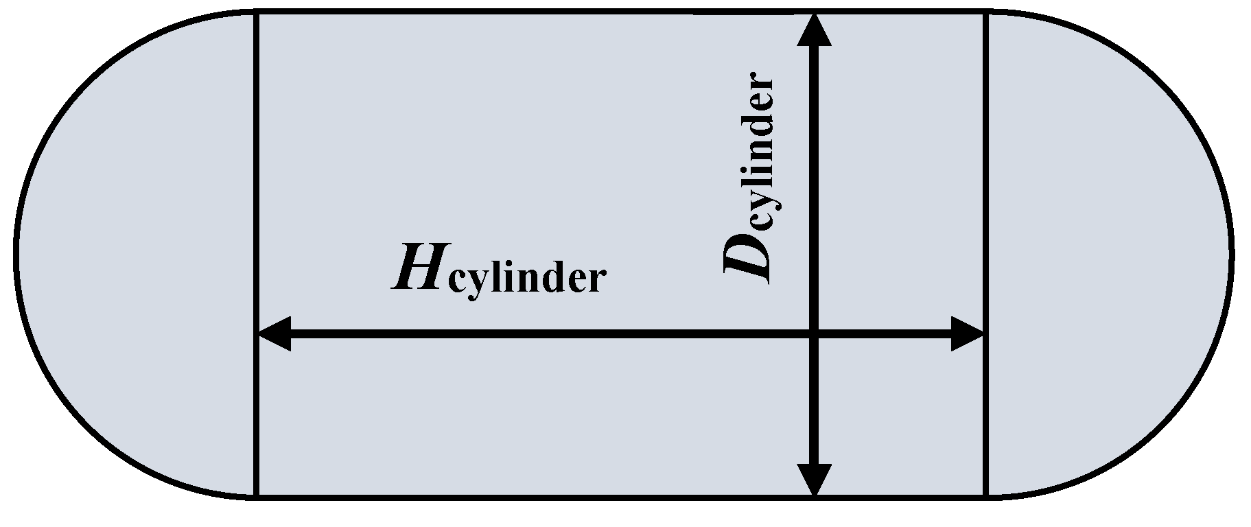
A fuel cell system generates a significant amount of waste heat that has to be removed with a cooling system, and this cooling system represents a significant part of the total system mass. For this reason, it is of utmost importance to minimize the mass of the cooling system. This can be achieved by using a two-phase cooling (2-PC) system. Figure 1 shows a schematic drawing of a 2-PC system. A pump transports liquid to an evaporator, which consists of cooling plates that are integrated in the fuel cell stack. In the evaporator, the waste heat from the fuel cells is absorbed and the liquid (partly) turns into vapour (i.e., the term ‘two-phase’ refers to the phase transition of the fluid from liquid to vapour). The vapour/liquid mixture then flows to the condenser. In the condenser, the absorbed heat from the Fuel Cell (FC) is transferred to the air that flows through the ram air heat exchanger (HX), and the vapour is turned back into liquid.
The schematic is very similar to that of a liquid Ethylene Glycol Water (EGW) cooling system that is commonly used for fuel cells, except that in a 2-PC the liquid is evaporated. This results in several advantages:
- The required mass flow is an order of magnitude smaller. This results in much lower electrical power consumption of the pump and a much smaller pump mass. Also, the piping diameter can be smaller, which reduces the overall mass of the system.
- Freezing of the fluid under low ambient temperatures (-55 °C) is not possible, since the freezing points of fluids that are used for two-phase cooling are much lower (typically lower than -80 °C) than the freezing point of EGW (approximately -45 °C).
- Due to the low freezing point and high heat transfer coefficient of two-phase fluids, it is easier to use the waste heat from the fuel cell to warm liquid H2 before it enters the fuel cell.
A disadvantage compared to liquid cooling is that the accumulator of a 2-PC has to be considerably larger. Also, the design is more complex.
1.3. Heat Source
A fuel cell stack (see Figure 2 (a) for a photo) consists of a large number (around 500) of Membrane Electrode Assembly (MEA) with metal bipolar plates on both sides (see Figure 2 (b)). H2 and O2 gas flow between the MEA and the bipolar plates, while the cooling channels are located between the bipolar plates. Fuel cells typically have an efficiency of ~55%. As a result, a 2.4 MW fuel cell system generates 2 MW of waste heat. The heat flux is typically around 1 W/cm2. Because a FC stack contains a complex system of gaskets and sealings to separate the air, hydrogen and coolant flows, the pressure of the coolant is limited to approximately 4 barg.
1.4. Heat Sink
The waste heat generated by the fuel cells has to be transported to a heat sink. In electric aircraft, the heat sink is the ambient air outside the aircraft. This air can have a temperature between -55 °C and +50 °C. The air is routed through a ram air heat exchanger. The air is forced through the heat exchanger by the aircraft’s forward motion or, when the aircraft is stationary, by a fan.
When liquid hydrogen (with a temperature of -250 °C) is used as energy carrier in electric aircraft it has to be warmed to ambient temperatures before it can enter the fuel cell stack. The warming can be achieved with an electric heater, but this costs approximately 8% of the electrical output of the fuel cell. Instead, the liquid hydrogen flow can also be used as an additional heat sink for the waste heat of a fuel cell.
2. Analyses Methods
In this section, the methods for the 2 MW cooling system analyses is discussed. The analysis starts with a fluid pre-selection. The most promising fluids are then analysed in more detail, after which the fluid is selected. In the analysis, the 2-PC system is also compared to a conventional cooling system with a liquid EGW mixture.
2.1. Fluid Preselection with ‘Figure of Merit’
For 2-PC, it is important that the tubing has a small diameter. Not only is the routing of the tubing much simpler when the diameter is small, but the system volume also scales with the square of the diameter, and a higher system volume results in a higher fluid mass and larger and heavier components. For this reason, it is important to minimize the diameter of the tubing. However, a small diameter of the tubing results in a large pressure drop. This pressure drop is not only disadvantageous for the pump power, but a large pressure gradient in a 2-PC system also results in a large temperature gradient (since pressure and boiling temperature are related). For this reason, an important characteristic of the fluid for 2-PC is a small pressure drop for a certain heat transport and geometry. The pressure drop in tubing is proportional to a fluid dependent part, a geometry dependent part (i.e., the length and diameter of a tube) and depends on the heat input [3]:
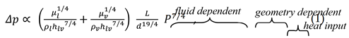
where μ is the fluid viscosity (with subscript l for liquid and subscript v for vapour), is the density, hlv is the heat of evaporation, L is the length of a tube, d the internal diameter, and P the heat input. The pressure gradient in the loop results in a gradient in the saturation temperature in the loop:
The inverse of the equation above can be used to find a fluid that results in a small temperature gradient (as a result of the pressure gradient). This inverse is called a figure of merit:
Figure 3 shows this figure of merit M for temperatures between 50° C and 130° C for all fluids in the NIST REFPROP [4] fluids database. On the horizontal axis, the saturation temperature of the fluid is shown. The FC have an operating temperature between 60° C and 100 °C. These temperatures are indicated with the dashed grey vertical lines. The pressure of a fluid increases with saturation temperature, and results with a saturation pressure above 5 bara (the maximum pressure for the fuel cell is 4 barg) are excluded, which is the reason why many lines are truncated above a certain temperature.
Methanol has the highest figure of merit, which means that the tubing diameter can significantly smaller than for other fluids. However, methanol is flammable and toxic. Figure 4 (b) shows the figure of merit with flammable fluids excluded. The best non-flammable fluids that can be used at the fuel cell operating temperatures are water, Novec 649, and C6F14 (perfluorohexane, also known as Fluorinert 72). Table 1 shows fluid properties of methanol and these non-flammable fluids. From the figures, it can be seen that methanol has about a 10 times higher figure of merit than e.g., C6F14. As a result, a 2-PC system with methanol can have smaller tubing diameter than with C6F14, which results in a lower mass of the system. This is further analyzed with the NLR system analysis tool, which is described in the next sections.
The saturation temperature has a large influence on the figure of merit of fluids because the pressure in the system becomes higher with higher saturation temperature, and this higher pressure results in a smaller vapour volume flow which results in smaller pressure differences. For FC operating above 120 °C, water becomes a very efficient two-phase fluid. When water is used as a two-phase cooling fluid, it would be possible to dump the water vapour directly into the ambient air during take-off on a hot day, instead of condensing water vapour back into liquid in the ram air HX. This would result in a much smaller ram air HX.
2.2. System Analysis Tool
In the next sections, the fluids listed in Table 2 are further analysed with the NLR cooling system analysis tool. Also, a system with liquid EGW is analysed and the calculated mass and power are compared to a 2-PC system. The system analysis software can calculate the steady-state and transient behaviour of two-phase and single-phase cooling systems and vapour compression cycles by numerically solving the 1D mass and enthalpy equations. The software also includes a cross-flow air-fluid heat exchanger. A detailed description of the model and the correlations for the pressure difference and heat transfer coefficient that are used in the model can be found in [6] and [7]. For the analyses, the following requirements are used:
- Total heat rejection during take-off: 2 MW
- Maximum power consumption (fans and pumps): 100 kW
- Air temperature during take-off: 30 °C
3. Results for Two-Phase Methanol
Figure 4 shows the calculated temperatures in the system for take-off conditions with methanol as coolant. Figure 5 and Figure 6 show the calculated vapour mass fraction and pressure. The input parameters for the model are indicated with red text, while the output is in black text. The mass flow is chosen such that 30% of the liquid is evaporated in the evaporator. All simulation parameters for the analysis are provided in Appendix A.1 while the geometry parameters are provided in Appendix A.2. The system contains 4 parallel ram air heat exchangers and there are 4 parallel groups of evaporators. The temperature at the condenser inlet is 4 °C lower than the evaporator outlet temperature as a result of the pressure difference between the evaporator and the condenser. This value can be reduced by increasing the diameter of the tubing, but this would increase the volume of the accumulator. The pressure at the inlet of the pump is 2.2 bara. The pump has an inlet temperature of 80°C, which means that the liquid methanol will start to boil below a pressure of 1.8 bara. The difference of 0.4 bar between the pump inlet pressure and the pressure at which the fluid starts to boil is the available NPSH (Net Positive Suction Head) for the pump. In order to prevent cavitation of the pump, the available NPSH must be larger than the minimal required NPSH. A typical required NPSH for a centrifugal pump is 0.3 bar. The total pressure drop over the pump is 1 bar. The pump power is 1.6 kW (assuming a pump efficiency of 50%). The required fan power is 98 kW (assuming a fan efficiency of 75%) and the total fan and pump power is just below the requirement of 100 kW. The mass and size of the air heat exchanger can be made smaller at the expense of higher fan power.
In Appendix B, the details for the mass estimation are provided. The total mass of the fluid (239 kg), tubing (35 kg), accumulator (32 kg), pump (11 kg), and heat exchanger (213 kg) is 529 kg. The mass of the fluid has a large contribution to the total mass of the cooling system. However, only a small fraction of this fluid mass is actually in the loop when the system is operational with a fuel cell heat load, since in that case, a large part of the system volume is filled with vapour and the excess liquid is stored in the accumulator. Conventional pumped two-phase cooling systems have an accumulator, but it is possible to have a 2-PC without accumulator [8]. In that case, the mass flow is scaled with the fuel cell heat load such that the vapour fraction in the system remains approximately constant. Without accumulator, a very large reduction in the system mass could be achieved, not only because of the absent accumulator, but primarily because of the large reduction in fluid mass. The total mass of a 2-PC system without accumulator is 297 kg (38 kg for fluid, 35 kg for tubing, 11 kg for the pump, and 213 kg for the heat exchanger). In order to investigate the feasibility of a system without accumulator, a 20 kW 2-PC system with methanol was built and successfully tested [9].
4. Results for Two-Phase Water
Figure 7 shows the calculated temperatures in the system for take-off conditions with water as two-phase coolant. The system parameters and geometry are exactly the same as for the simulation for methanol, except for the following differences:
- FLUID.name=‘water’ instead of ‘methanol’, see Appendix A
- constant.d_twophase=178e-3 instead of 114e-3
- constant.d_liquid=constant.d_twophase*0.25 instead of constant.d_liquid=constant.d_twophase*0.4
Water has a high heat of evaporation (see Table 1), which means that the required water volume flow is very small compared to methanol (183 l/min versus 463 l/min). However, the absolute pressure of water at a boiling temperature of 95 °C is just 0.8 bar, which means that the pressure drop over the system has to be kept relatively small. As a result, the diameter of two-phase tubing has to be larger than for methanol, which results in a higher fluid mass. The total calculated system mass with two-phase water is 840 kg, which is higher than for methanol (529 kg). Water is therefore not a good fluid for two-phase cooling of fuel cells at 95°C (but it becomes a good fluid >120°C).
5. Results for Liquid EGW Mixture
In the previous sections, 2-PC systems were analysed. In this section, a cooling system with liquid EGW mixture is analysed. The system parameters and geometry are exactly the same as for the simulation for two-phase methanol, except for the following differences:
- FLUID.cooling_type=1 instead of 2 (2=two-phase cooling, 1=liquid cooling)
- FLUID.name=‘water-eglycol’ (40-60% mixture) instead of ‘methanol’
- constant.d_twophase=97e-3 instead of 114e-3
- The size of the air HX in the direction of the airflow is increased with 10%: HX.L = 0.21*1.1 instead of 0.21
- The width of the air HX is increased with 15%: HX.W = 0.75*1.154 instead of 0.75
Figure 8 shows the calculated temperatures in the system for take-off conditions for a liquid EGW cooling system. The liquid flow for the EGW cooling system is chosen such that the increase in liquid temperature over the fuel cell is 15 °C. The volume flow is 5 times larger than for a 2-PC with methanol. Also, the pressure drop over the pump is larger. As a result, the required pump power is 12.9 kW compared to 1.6 kW for methanol. Because of the higher pump power, the air HX is made slightly larger in order to decrease the pressure drop over the air HX and thereby reduce the fan power to 90 kW in order not to exceed too much the 100 kW requirement for fan + pump. The ram air HX is dimensioned such that the liquid temperature at the exit of the fuel cell is 95° C, which requires a small increase in the air HX size because the average fluid temperature in the heat exchanger is slightly lower compared to a 2-PC, and the heat transfer coefficient for liquid EGW is lower than for two-phase methanol.
The inner diameter of the tubing of a liquid EGW system (97 mm) is much larger than the liquid tubing diameter in a 2-PC with methanol (46 mm) but slightly smaller than the two-phase tubing diameter with methanol (114 mm).
The accumulator for a liquid cooling system can be relatively small (since it only has to compensate for density changes of the liquid due to temperature variations) and the mass of this vessel is neglected in the analysis. For a liquid EGW cooling system, the total mass of the fluid (355 kg), tubing (45 kg), pump (53 kg), and heat exchanger (263 kg) is 716 kg, which is 35% higher than for two-phase methanol with accumulator (529 kg) and 2.4 times higher than for two-phase methanol without accumulator (297 kg).
6. Discussion and Conclusion
Table 2 shows the summary of the analysis results. For a 2-PC, using methanol results in a system mass of 529 kg for a conventional system and 297 kg for the system without accumulator. Using a non-flammable alternative results in much higher system mass. A cooling system with a liquid EGW mixture has also been analysed. These results are included in the right column of Table 2. The mass of a liquid EGW system is 716 kg, which is 35% higher than for two-phase methanol with accumulator (529 kg) and 2.4 times higher than for two-phase methanol without accumulator (297 kg). In order to investigate the feasibility of a system without accumulator, a 20 kW 2-PC system with methanol was built and successfully tested [9].
Besides the high system mass with the non-flammable fluids Novec 649 and Fluorinert 72, concerns have been raised recently about the environmental impact of PFAS (Per- and polyfluoroalkyl substances) [10]. There is currently a proposal from the European Chemical Agency to restrict PFAS, including refrigerants [11]. In this proposal, there are exceptions for the restrictions, e.g., “refrigerants in HVACR-equipment in buildings where national safety standards and building codes prohibit the use of alternatives” and “refrigerants in transport refrigeration other than in marine applications”. However, even if there would be an exception, manufacturers might decide to stop producing this refrigerant anyway. This might impact future availability of Novec 649, Fluorinert 72 or other engineered refrigerants.
Author Contributions
Conceptualization, W. Resende, G. Mühlthaler, and M.B. Buntz; methodology, H.J. van Gerner; software, H.J. van Gerner, T. Luten; validation, H.J. van Gerner; formal analysis, H.J. van Gerner; investigation, H.J. van Gerner; resources, H.J. van Gerner; data curation, H.J. van Gerner; writing—original draft preparation, H.J. van Gerner; writing—review and editing, T. Luten, G. Mühlthaler and M.B. Buntz; visualization, H.J. van Gerner, T. Luten; supervision, H.J. van Gerner; project administration, H.J. van Gerner; funding acquisition, H.J. van Gerner. All authors have read and agreed to the published version of the manuscript.
Funding
This BRAVA project is funded by the European Union’s Horizon under grant agreement number 10110149. This publication reflects the authors’ views. Neither the European Union nor the Clean Hydrogen Joint Undertaking can be held responsible for them.

Data Availability Statement
The input parameters for the simulations described in the study are included in the appendixes of the article. Further inquiries can be directed to the corresponding author/s.
Conflicts of Interest
The funders had no role in the design of the study; in the collection, analyses, or interpretation of data; in the writing of the manuscript; or in the decision to publish the results.
Appendix A Input for System Analysis
Appendix A.1 Simulation Parameters
%% Simulation settings
FLUID.cooling_type=2; % 2=two-phase, 1=liquid
FLUID.name=‘methanol’; % Fluid in system, if mixture (only for liquid cooling): always split by: -
FLUID.mix=[0.4 0.6]; % fraction of mixture (only for liquid cooling): first fraction is for first fluid in FLUID.name
system=‘Airbus’; % Geometry of system
%% Initial values and conditions
constant.P(1:4)=500e3; % Heat input per Fuel Cell branch [W]
constant.nrBranch=length(constant.P); % number of evaporator branches
constant.nrCondens=4; % number of condensers
constant.nrCondensAir=20; %non-physical division of condenser in several parallel tubes (for the cross-air heat exchanger).
constant.NRiter=150; % NR of iterations
constant.CalcParallel=0; % if 1, calculate distribution, if 0, assume equal distribution over parallel branches
constant.dP_cor=1; % Two-phase frictional pressure drop correlation. 1=Muller-Steinhagen&Heck, 2=Friedel
constant.Xexit=0.3; % vapour mass fraction after evaporator
constant.DTpreheat=15; %For liquid, this is the temperature increase due to the heat load, for two-phase, this determines the preheater power (if present in system)
constant.Tkelvin=273.15; % zero degrees Celsius [K]
constant.Tsp=95+constant.Tkelvin;% set-point temperature [K]
constant.Tsink=30+constant.Tkelvin; % heat sink (i.e., space or ambient air) temperature [K]
constant.Tinit=constant.Tsink ; % initial temperature of the loop [K]
constant.pump_eff=0.5; % adiabatic efficiency of pump [-]
constant.fan_eff=0.75; % adiabatic efficiency of pump [-]
constant.Recuperator=0; % 1=with recuperator, 0=without recuperator
%% accu properties
accu.Tmax=110+constant.Tkelvin; % maximum temperature used for strength and mass calculation
accu.Hratio=1.5; % ratio between the height of the cylindrical part and the diameter of the accumulator, e.g., Hratio=H/D
accu.material=‘aluminium’;
accu.rho=2700;% density [kg/m^3]
accu.factor_proof=3; % factor for proof pressure
accu.factor_burst=4; % factor for burst pressure
accu.Smargin=1.25; %additional margin factor for proof and burst calculation
accu.Syield=83e6; %yield strength [N/m2]
accu.Sultimate=110e6; %ultimate strength [N/m2]
%% ambient air input
air.InputType=1 ; % if InputType=1, air mass flow is input. if InputType=2, air mass flow is calculated from air speed
air.m = 44.7/4; % air massflow [kg/s] (only for air.InputType=1)
air.U = 230/3.6; % flight speed in [m/s] (only for air.InputType=2)
air.pin = 1e5; % ambient air pressure [Pa]
air.Tin = constant.Tsink; % Ambient air temperature; HX inlet air temperature
air.Tout = air.Tin+30; % Initial guess for HX outlet air temperature
%% Finned air HX properties
HX.L = 0.21; % Length of HX [m]: from air inlet to air outlet
HX.Wlayer = 0.75*1.03; % Width of HX layer of fins [m]
HX.NRlayer = 44; % number of layers of fins
HX.W = HX.Wlayer*HX.NRlayer; %: width of HX times number of layers of fins
HX.Hfin = 15e-3; % Height of one fin [m]
HX.tfin = 0.15e-3; % Thickness of one fin [m]
HX.dfin = 0.82e-3; % Distance between two fins [m]
HX.k = 167; % Thermal conductivity of material btwn condenser-tube and airHX [W/mK]
HX.rho = 2700; % Density of material btwn condenser-tube and airHX [kg/m3]
HX.K_inlet = 0.0; % Minor pressure loss at air inlet of HX
HX.K_outlet = 0.0; % Minor pressure loss at air inlet of HX
Appendix A.2 Geometry Parameters
%########################################################################%
%# #%
%# Geometry of Airbus two-phase cooling MPL #%
%# #%
%########################################################################%
%# #%
%# Components are structured like this: #%
%# <ID> = Identifier number #%
%# <Name> = Component name #%
%# ‘L’ = Length of component [m] #%
%# ‘D’ = Diameter of component [m] #%
%# ‘D_restriction’ = Diameter of restriction [m], 0 for no restriction #%
%# ‘nParTube’ = Number of parallel tubes [-] #%
%# ‘Shape’ = Geometrical shape of tubes. 0 for round, 1 for square #%
%# ‘Diab’ = 0 for none, 1 for evaporator, 2 for HX, #%
%# 3 for condenser, 4 for single-phase #%
%# ‘mass’ = Mass of component [kg] #%
%# ‘Cp’ = Specific heat of material [J kg-1 K-1] #%
%# ‘K’ = minor loss coefficient #%
%# ‘nElm’ = Number of elements per component #%
%# ‘e’ = Pipe inner roughness #%
%########################################################################%
constant.d_twophase=114e-3; % [m] inner diameter of two-phase tubing
if FLUID.cooling_type==1
constant.d_liquid=constant.d_twophase; % [m] inner diameter of liquid tubing
else
constant.d_liquid=constant.d_twophase*0.4; % [m] inner diameter of liquid tubing
end
d_condenser=1.4e-3; % [m] inner diameter of condenser tubes
d_factor=constant.d_twophase/114e-3; % scaling factor for diameter of condenser, etc.
restriction_factor=1;
%% Minor pressure loss constants
% From: Y. A. Çengel, Fundamentals of thermal-fluid Sciences (McGraw-Hill, New York, 2012).
K_elbow=1.1;
K_union=0.08;
K_tee_b=2; % Branch flow
K_tee_l=0.9; % Line flow
K_long_bend=0.3;
K_inlet=0.5; % inlet loss
K_outlet=1; % outlet loss
nC=0; % Start counting the number of components
%% Tube from pump to Evap
nC=nC+1;
name=‘Tube_PtoE’;
ID.(name)=nC;
C(nC)=struct(‘ID’,name, ‘L’,5, ‘D’,constant.d_liquid,‘D_restriction’,0.0e-3, ‘nParTube’,1, ‘K’,K_outlet+K_long_bend*2,‘e’,2e-6, ‘Shape’,0, ‘Diab’,0, ‘mass’,1, ‘Cp’,1);
for i=1:constant.nrBranch %% START evaporator branches
d_restriction=constant.d_liquid*restriction_factor; % add restriction to inlet of each branch
%d_restriction=0;
%% tube to Evaporator that contains the restriction
nC=nC+1;
name=‘Tube_toE’;
ID.(name)(i)=nC;
C(nC)=struct(‘ID’,[name ‘‘ int2str(i)], ‘L’,0.1, ‘D’,constant.d_liquid,‘D_restriction’,d_restriction, ‘nParTube’,1, ‘K’,K_outlet,‘e’,2e-6, ‘Shape’,1, ‘Diab’,0, ‘mass’,1, ‘Cp’,1);
%% Evaporator
nC=nC+1;
name=‘Evaporator’;
ID.(name)(i)=nC;
% cooling channels in FC biploar plates
C(nC)=struct(‘ID’,[name ‘‘ int2str(i)], ‘L’,0.370, ‘D’,0.62e-3,‘D_restriction’,0, ‘nParTube’,88*500*5, ‘K’,0,‘e’,2e-6, ‘Shape’,1, ‘Diab’,1, ‘mass’,40, ‘Cp’,900);
%% tube from Evaporator
nC=nC+1;
name=‘Tube_fromE’;
ID.(name)(i)=nC;
C(nC)=struct(‘ID’,[name ‘‘ int2str(i)], ‘L’,0.1, ‘D’,constant.d_twophase,‘D_restriction’,0, ‘nParTube’,1, ‘K’,K_outlet,‘e’,2e-6, ‘Shape’,1, ‘Diab’,0, ‘mass’,1, ‘Cp’,1);
end
ID.twophase_start=ID.Evaporator(1);
%% Tube from Evaporator to Condenser
nC=nC+1;
name=‘Tube_EtoC’;
ID.(name)=nC;
C(nC)=struct(‘ID’,name, ‘L’,10, ‘D’,constant.d_twophase,‘D_restriction’,0, ‘nParTube’,1, ‘K’,(K_inlet+K_outlet+K_long_bend*2)*1,‘e’,2e-6, ‘Shape’,0, ‘Diab’,0, ‘mass’,1, ‘Cp’,1);
for i=1:constant.nrCondens %% START branches
%% tube to condenser
nC=nC+1;
name=‘Tube_toC’;
ID.(name)(i)=nC;
C(nC)=struct(‘ID’,[name ‘‘ int2str(i)], ‘L’,0.1, ‘D’,constant.d_twophase,‘D_restriction’,0, ‘nParTube’,1, ‘K’,K_outlet,‘e’,2e-6, ‘Shape’,1, ‘Diab’,0, ‘mass’,1, ‘Cp’,1);
for j=1:constant.nrCondensAir
%% Condenser
nC=nC+1;
name=‘Condenser’;
ID.(name)(i,j)=nC;
C(nC)=struct(‘ID’,[name ‘_’ int2str(i) ‘_’ int2str(j)], ‘L’,HX.Wlayer, ‘D’,d_condenser*d_factor,‘D_restriction’,0, ‘nParTube’,HX.L*HX.NRlayer/(d_condenser*d_factor)/1.1/constant.nrCondensAir, ‘K’,0,‘e’,2e-6, ‘Shape’,0, ‘Diab’,3, ‘mass’,80, ‘Cp’,900);
end
%% tube to condenser
nC=nC+1;
name=‘Tube_fromC’;
ID.(name)(i)=nC;
C(nC)=struct(‘ID’,[name ‘‘ int2str(i)], ‘L’,0.1, ‘D’,constant.d_liquid,‘D_restriction’,0, ‘nParTube’,1, ‘K’,K_outlet,‘e’,2e-6, ‘Shape’,1, ‘Diab’,0, ‘mass’,1, ‘Cp’,1);
end
ID.twophase_end=ID.Condenser(end,end);
%% Tube from condenser to accu
nC=nC+1;
name=‘Tube_CtoA’;
ID.(name)=nC;
C(nC)=struct(‘ID’,name, ‘L’,5, ‘D’,constant.d_liquid,‘D_restriction’,0, ‘nParTube’,1, ‘K’,(K_inlet+K_tee_l+K_long_bend*2)*0,‘e’,2e-6, ‘Shape’,0, ‘Diab’,0, ‘mass’,1, ‘Cp’,1);
ID.preAccu=nC; % index for last component before accu
%% Tube from accu to pump
nC=nC+1;
name=‘Tube_AtoP’;
ID.(name)=nC;
C(nC)=struct(‘ID’,name, ‘L’,1, ‘D’,constant.d_liquid,‘D_restriction’,0, ‘nParTube’,1, ‘K’,(K_inlet+K_tee_l+K_long_bend*2)*1,‘e’,2e-6, ‘Shape’,0, ‘Diab’,0, ‘mass’,1, ‘Cp’,1);
Appendix B Mass Estimation
In this appendix, the method for estimating the mass of several components is explained.
Appendix B.1 Accumulator Vessel
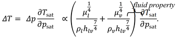
Figure A1 shows a schematic drawing of an accumulator vessel. It consists of a cylinder with two caps. In the simulations, it is assumed that the ratio between Hcylinder and Dcylinder is 1.5 (see accu.Hratio=1.5 in Appendix A.1). The minimum volume of an accumulator is equal to the volume of the system between the evaporator inlet and the condenser outlet (i.e., the part of the system where vapour can occur) plus the volume of the liquid needed for expansion due to temperature variations.
The volume of the accumulator consists of the volume of the cylinder:
and the volume of the spherical caps:
From these equations, the required diameter and height of the accumulator is calculated. The wall thickness t of the cylinder and caps of the vessel are then calculated with the pressure vessel equations:
where pproof/burst is the proof or burst pressure for the vessel. For the wall thickness calculation for the proof pressure, the yield strength σyield of the vessel wall is used, while for the wall thickness calculation for the burst pressure, the ultimate strength σultimate is used. The factor Smargin is an additional safety margin. In the analysis, this margin is 1.25 (see accu.Smargin=1.25 in Appendix A.1).
Figure A1.
Schematic drawing of an accumulator vessel.
Appendix B.2 Tubing
The mass of the tubes is calculated with:
where Ltube is the length of the tube, dtube is the diameter, twall is the wall thickness of the tube, and ρ is the density of the tube wall. It assumed that aluminium tubes are used, so the density is 2700 kg/m3. The thickness of the tube wall increases with the diameter. The thickness of the wall in mm is approximated with:
Appendix B.3 Pump
The mass of the pump in kg is calculated with:
where is the volume flow of the pump in litres/minute.
Appendix B.4 Fluid
The total fluid mass in the system is equal to the total volume of the system multiplied by the liquid density of the fluid.
Appendix B.4 Ram Air Heat Exchanger
The mass of the ram air heat exchanger consists of the mass of the aluminium fins (see ‘Finned air HX properties’ in Appendix A.1) and plates with coolant channels. The air and fluid manifolds are not included in the mass estimation.
References
- EKPO Fuel cell stacks. Available online: https://www.ekpo-fuelcell.com/en/products-technology/fuel-cell-stacks (accessed on 22 10 2024).
- Neto, D.M.; Oliveira, M.C.; Alves, J.L.; Menezes, L.F. Numerical study on the formability of metallic bipolar plates for Proton Exchange Membrane (PEM) Fuel Cells. Metals 2019, vol. 9, p. 810.
- van Gerner, H.J.; van Benthem, R.C.; van Es, J.; Schwaller, D.; Lapensée, S., Fluid selection for space thermal control systems. 44th International Conference on Environmental Systems 2014.
- Lemmon, E.; Huber, M.; McLinden, M. NIST Standard Reference Database 23: Reference Fluid Thermodynamic and Transport Properties-REFPROP, Version 9.1,” National Institute of Standards and Technology, Standard Reference Data Program, Gaithersburg.
- NFPA 704 Standard System for the Identification of the Hazards of Materials for Emergency Response. Available online: https://www.nfpa.org/Codes-and-Standards/All-Codes-and-Standards/List-of-Codes-and-Standards. (accessed on 18 02 2021).
- van Gerner, H.J.; Braaksma, N.; Transient modelling of pumped two-phase cooling systems: Comparison between experiment and simulation, ICES-2016-004. 46th International Conference on Environmental Systems 2016.
- van Gerner, H.J.; Bolder, R.; van Es, J. Transient modelling of pumped two-phase cooling systems: Comparison between experiment and simulation with R134a, ICES-2017-037. 47th International Conference on Environmental Systems 2017.
- Donders, S. N. L.; Banine, V. Y.; Moors, J. H. J; Verhagen, M. C. M.; Frijns, O. V. W.; van Donk, G.; van Gerner, H. J. Thermal conditioning system for thermal conditioning a part of a lithographic apparatus and a thermal conditioning method, Patent US8610089, 2013.
- van Gerner, H.J.; Luten, T.; Scholten, S; Mühlthaler, G.; Buntz, M.B. Test results for a novel 20 kW two-phase pumped cooling for aerospace applications. Energies 2024. (not yet published).
- PFAS ban affects most refrigerant blends. Available online: https://www.coolingpost.com/world-news/pfas-ban-affects-most-refrigerant-blends/ (accessed on 20 April 2023).
- ECHA, European Chemical Agency; Submitted restrictions under consideration. Available online: https://echa.europa.eu/restrictions-under-consideration/-/substance-rev/72301/term (accessed on 24 January 2024).
Figure 1.
Schematic drawing of a 2-PC.
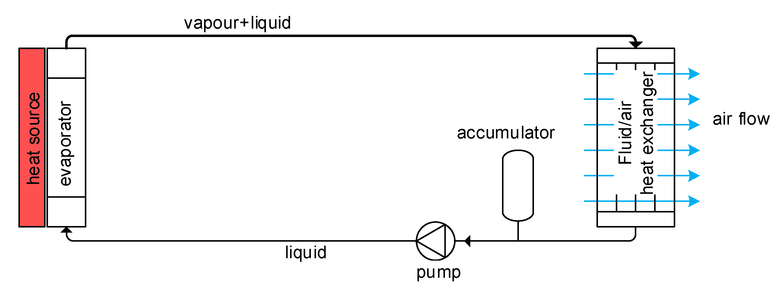
Figure 2.
(a) Photo of a Fuel Cell stack [1]; (b) Cross-section of a single layer in a fuel cell stack [2].
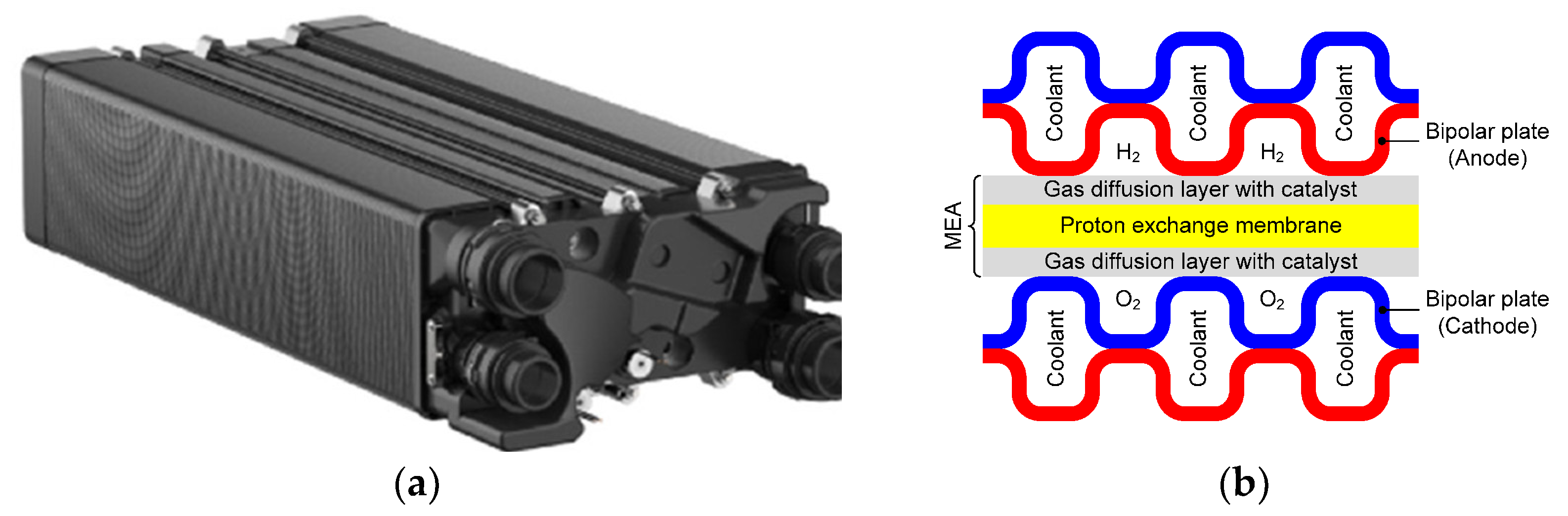
Figure 3.
Figure of merit: (a) all fluids in the REFPROP database, (b) excluding flammable fluids.
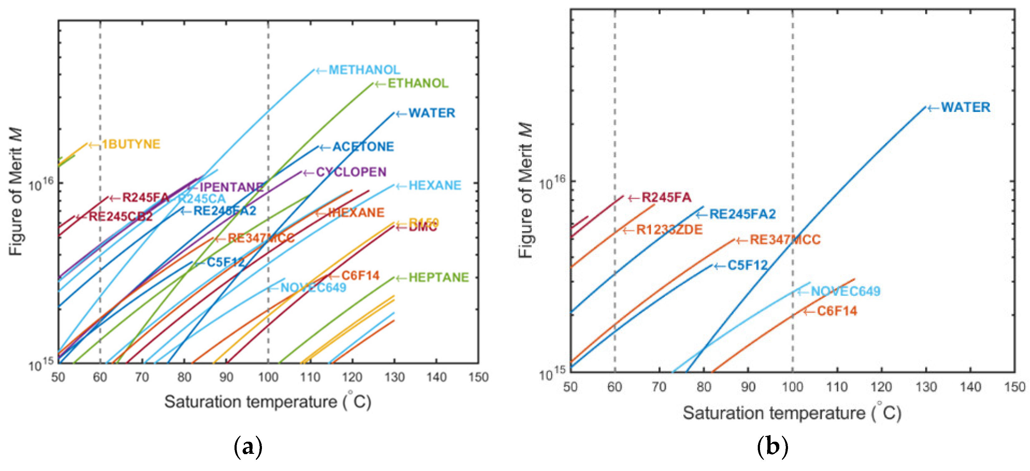
Figure 4.
Calculated temperatures for two-phase methanol.
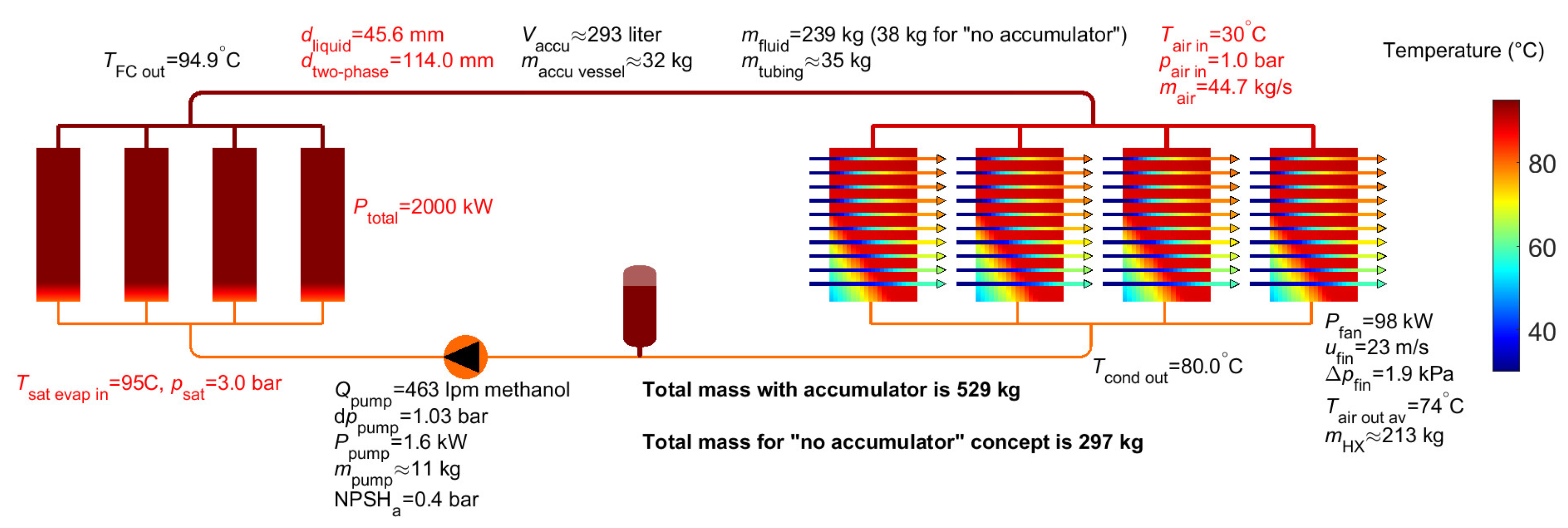
Figure 5.
Calculated vapour mass fraction for two-phase methanol.
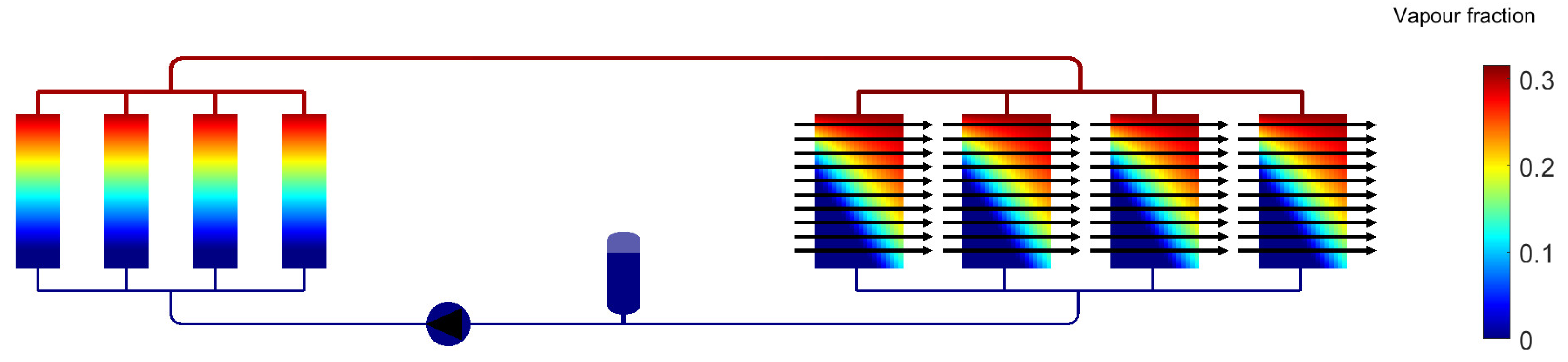
Figure 6.
Calculated pressures for two-phase methanol.
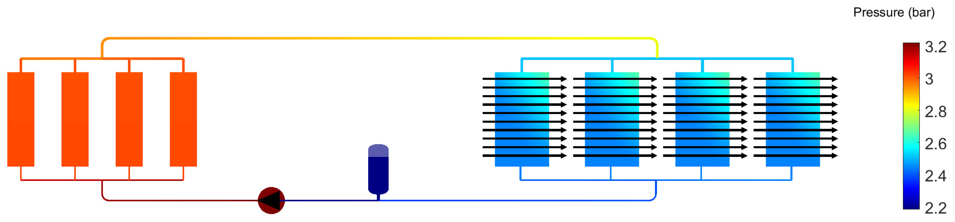
Figure 7.
Calculated temperatures for two-phase water.
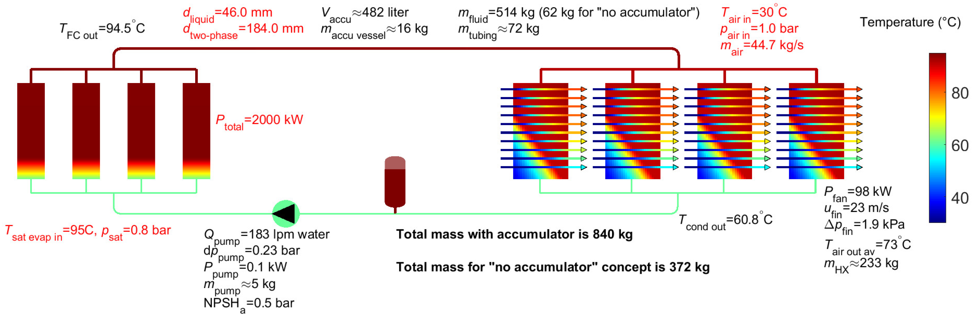
Figure 8.
Calculated temperatures for liquid EGW.
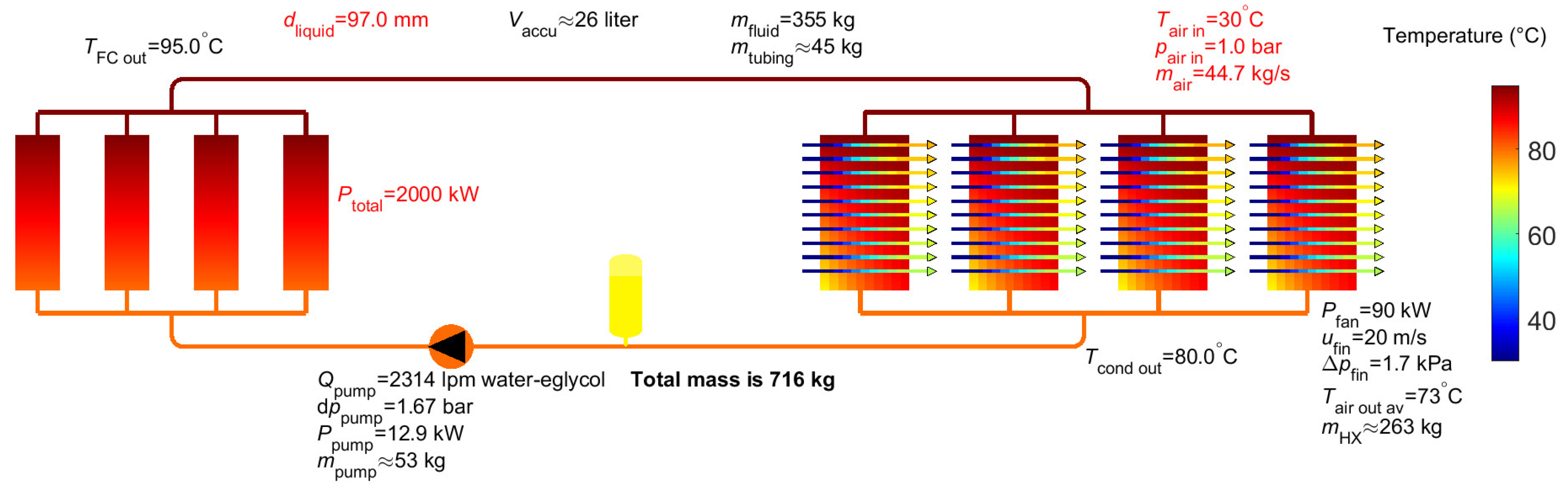

Table 1.
Relevant properties at 95 °C for preselected fluids.
| Methanol | RE347mcc (HFE-7000) | water | Novec 649 | Fluorinert 72 (C6F14) | |
| NFPA (health-flammability) [5] | 1-3 | 31-0 | 0-0 | 31-0 | 1-0 |
| Global Warming Potential | ~0 | 530 | ~0 | 1 | 9300 |
| Saturation pressure at 95 °C (bara) | 3.0 | 6.0 | 0.8 | 3.9 | 3.1 |
| Saturation pressure at 60 °C (bara) | 0.85 | 2.4 | 0.20 | 1.5 | 1.1 |
| Saturation pressure at 20 °C (bara) | 0.13 | 0.59 | 0.02 | 0.33 | 0.24 |
| Triple point (°C) | -97 | -122 | 0 | -108 | -86 |
| Heat of evaporation hlv (kJ/kg) | 1035 | 104 | 2270 | 72 | 73 |
| Specific heat Cp (kJ/kgK) | 3.1 | 1.4 | 4.2 | 1.2 | 1.2 |
| Liquid density ρl (kg/m3) | 717 | 1184 | 962 | 1361 | 1446 |
| Density ratio ρl/ρv | 208 | 24 | 1915 | 28 | 36 |
| conductivity kl (W/m K) | 0.19 | 0.05 | 0.68 | 0.05 | 0.06 |
| ∂Tsat/∂psat (°C/bar) | 10.1 | 6.8 | 31.8 | 9.9 | 12.2 |
Table 2.
Summary table for the different fluids.
| Methanol | water | Novec 649 | Fluorinert 72 (C6F14) | Liquid EGW | |
| Accumulator volume2 | 293 litres (-) | 482 litres (-) | 476 litres (-) | 542 litres | 26 litres |
| Pump flow | 463 lpm | 183 lpm | 1741 lpm | 1635 lpm | 2314 lpm |
| Pump power | 1.6 kW | 0.1 kW | 6.6 kW | 4.2 kW | 12.9 kW |
| Triple point (°C) | -97 °C | 0 °C | -108 °C | -86 °C | ~ -48 °C |
| Mass fluid2 | 239 kg (38 kg) | 514 kg (61 kg) | 810 kg (260 kg) | 992 kg (311 kg) | 355 kg |
| Mass tubing | 35 kg | 72 kg | 75 kg | 91 kg | 45 kg |
| Mass pump | 11 kg | 5 kg | 40 kg | 38 kg | 53 kg |
| Mass accumulator2 | 32 kg (-) | 16 kg (-) | 61 kg (-) | 56 kg (-) | neglected |
| Mass air heat exchanger | 213 kg | 233 kg | 226 kg | 232 kg | 263 kg |
| Total mass2 | 529 kg (297 kg) | 840 kg (372 kg) | 1212 kg (601 kg) | 1409 kg (671 kg) | 716 kg |
| 1 | The NFPA health safety classification code of 3 is due to emergency situations where the material may thermally decompose and release Hydrogen Fluoride. Under normal conditions, HFE-7000 and Novec 649 are non-toxic. |
| 2 | The value between brackets is for the ‘no accumulator’ concept. |
Disclaimer/Publisher’s Note: The statements, opinions and data contained in all publications are solely those of the individual author(s) and contributor(s) and not of MDPI and/or the editor(s). MDPI and/or the editor(s) disclaim responsibility for any injury to people or property resulting from any ideas, methods, instructions or products referred to in the content. |
© 2024 by the authors. Licensee MDPI, Basel, Switzerland. This article is an open access article distributed under the terms and conditions of the Creative Commons Attribution (CC BY) license (http://creativecommons.org/licenses/by/4.0/).
Copyright: This open access article is published under a Creative Commons CC BY 4.0 license, which permit the free download, distribution, and reuse, provided that the author and preprint are cited in any reuse.


