Submitted:
05 December 2024
Posted:
06 December 2024
Read the latest preprint version here
Abstract
The cosmological parameters, specifically BCP(Baryon Cosmological Parameter (Telescopic Universe) )and DCP (Dark Cosmological Parameters (Lightless Universe)), are accelerating more apace than we expected. This accelerated our understanding of its functions in covariance to expansion parameters[1]. The Hubble tension is a long-familiar question in the exploration of cosmological parameters[2][3]. The measurement of the Hubble constant (H0), unveils a disparity in how apace the BCP and DCP[4]. Diametrical ways of measuring parameters yield various results, highlighting the realness that numerous questions in this domain remain unanswered[5][6]. This gap brings to light question regarding our existing cosmological parameters known(CDM) [7][8]. It suggests the necessity of incorporating new parameters, often referred to as the DPP(Dark Physics Parameters) method, to gain an understanding of the accelerated universe. This theory integrates a between the Hubble equation, both BCP and DCP are accelerating cosmological Hubble parameters. This integration pertains to how Cosmological Hubble parameters evolve across the past, present, and future dimensions. We propose that both BCP and DCP are influenced by stochastic variables in a diametrical domain characterized by dissent magnitude of matter. This theory's conjunctive mass term, volume term, and CHP provide a new perspective on BCP, specifically DCP and Hubble Tension. This theory discusses that the reevaluation of our current understanding of BCP and DCP is necessary to integrate this acceleration of Universe Expansion changes. This adjustment could help us understand one of the biggest mysteries in modern cosmology.
Keywords:
Dark Energy
; Inflation
; Accelerate Universe
; Hubble Tension
1. Introduction
The attitude of CDP8 is pivotal in the study of detectable cosmological parameter. The equation that illustrates this balance parameter looks like this:
The theory of the CDP illustrates a distinction between two categories of universe parameters. The first category, referred to as the CUP9, the second category known as the OUP10. The term “normal density” is used to refer to [9] attentiveness the underway quantity of matter latter-day in the universe.
We formally compare normal density and CDP to ascertain the value of H0:
The subsequent expression is indicative of a constant
We consider the volume to be integral to the expansion series, which is represented in the following form:
If the universe dominate a distinct magnitude of space11, within the context of cosmology, this theory intend that Ho is not a static parameter, rather fluctuates in outcome to consequence in both BCP and DCP. As the parameter of the ]AUE ; the aspect of the both attribute and mass also experience maturation, leading to stochastic variable in the ]CHP. This dynamics interplay intensify our understanding of the cosmological principles dominant the ]CHP.
Hubble equation:
The final equation pertaining to the acceleration of the universe:
Figure 1.
PVEP. The graph titled "Positive Volume Expansion Series" illustrates the behavior of a volume expansion series across various term indices (n) against a beige grid background. The x-axis represents the term index, which extends from 0 to 10, while the y-axis quantifies the "Volume Value" in units of 101810^{18}, encompassing both positive and negative values. The data points, clearly marked with a green line and accompanying dots, display a consistent trend from n=0 to n=4, maintaining values close to zero. A significant shift is observed at n=5, where the values experience a sharp increase, ultimately peaking at approximately 4×10184×10^{18} at n=6. This ascent is followed by a rapid decline, leading to values dropping below zero, with a minimum reaching approximately -6×10^{18} at n=8. As the graph approaches n=10, there is a slight recovery, indicating an upward trend in values. The legend, located in the lower-left corner, designates the data as the"Positive Volume Expansion Series."This graph effectively demonstrates the transition of the positive series from stability to pronounced fluctuations, emphasizing its peaks and troughs and thereby providing valuable insights into its dynamic behaviour.
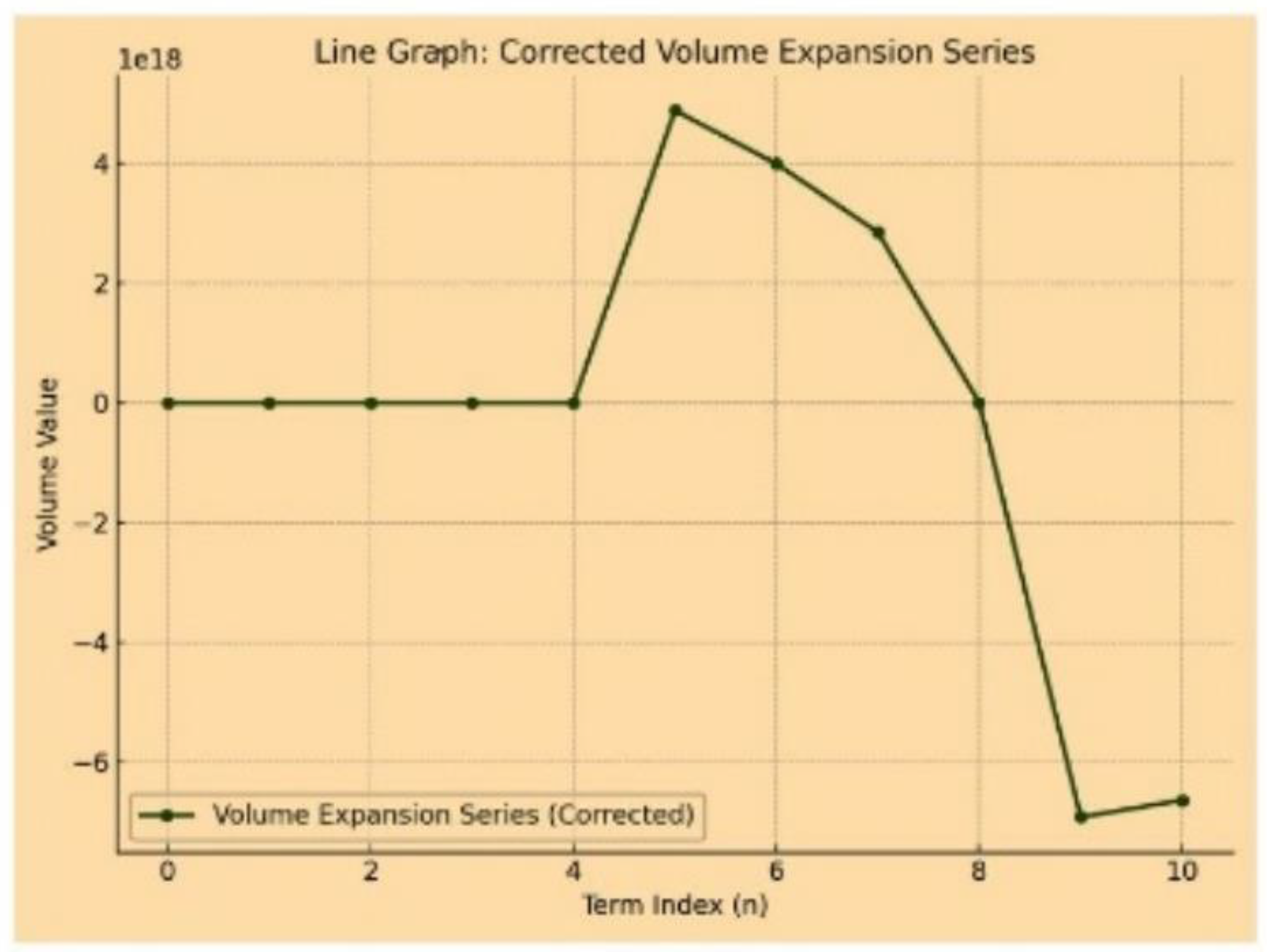
Figure 2.
NVEP. The graph titled "Negative Volume Expansion Series" visually represents the behavior of a volume expansion series across various term indices (n) on an aesthetically pleasing pink background grid. The horizontal axis (x-axis) indicates the term indices, ranging from 0 to 10, while the vertical axis (y-axis) denotes the corresponding "Volume Value," which spans from approximately -6 × 10¹⁸ to 6 × 10186 × 10¹⁸. The data points are plotted using a blue line, with distinct dots marking each data point for clarity. The trend illustrated in the graph reveals a noteworthy progression. From n=0 to n=4, the values remain stable, hovering around zero, indicating a period of consistency. However, a significant shift occurs at n=5, where the volume value experiences a steep decline, reaching a notable minimum of approximately -6 × 10¹⁸ at n=6. Following this decline, the graph demonstrates a rapid recovery, with values increasing sharply to peak at around 6 × 10186 × 10¹⁸ by n=9, maintaining this elevated level through n=10. The legend, positioned in the upper left corner, labels the series as "Negative Volume Expansion Series," which enhances interpretation of the data. This graph effectively illustrates the transition from a stable state to marked fluctuations, showcasing a substantial dip followed by a remarkable recovery within the specified term indices.
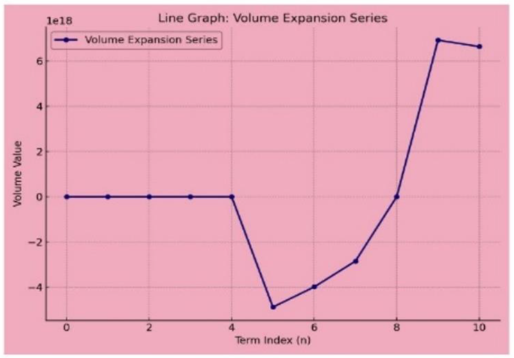
Figure 3.
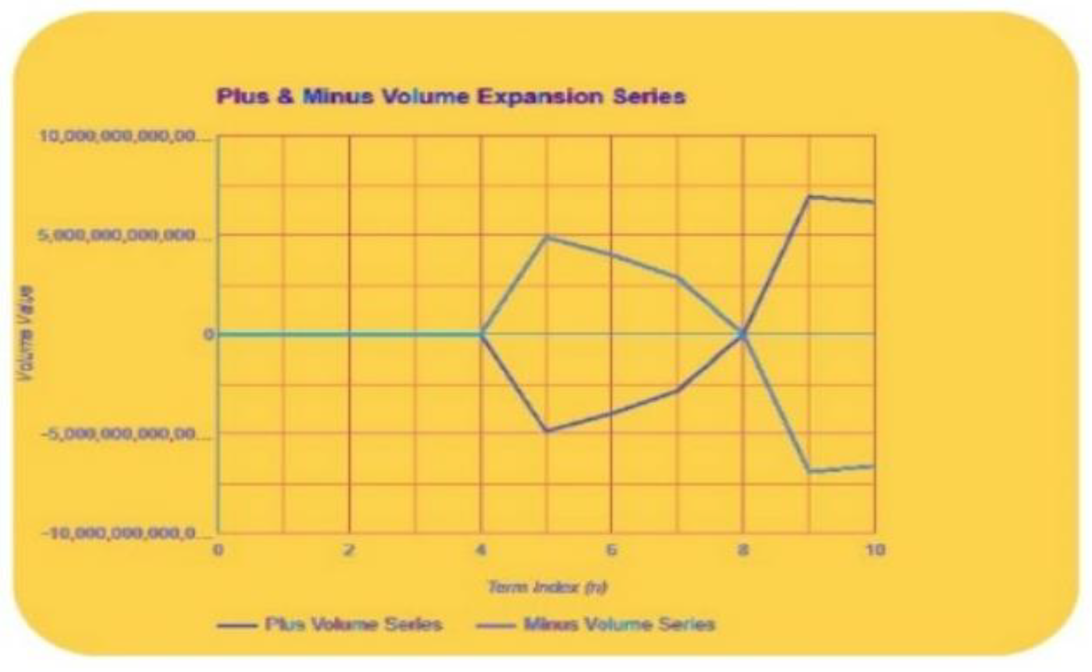
PVEP and NVEP volume expansion series. The graph titled "PVEP and NVEP Volume Expansion Series" presents an analysis of two opposing volume series, identified as the PVEP Series and the NVEP Volume Series, plotted against term indices ranging from 0 to 10. The horizontal axis denotes the term index (n), while the vertical axis illustrates the corresponding "Volume Value," which ranges from -10,000,000,000,000 to 10,000,000,000,000. The graph features a striking yellow background with a grid to enhance data interpretation. The two data series are clearly distinguished by colour: blue represents the Plus Volume Series and orange represents the Minus Volume Series. Initially, the PVEP Volume Series exhibits a stable trend, remaining close to zero for the early-term indices. However, it experiences a significant increase after n=5, reaching noteworthy positive values while displaying minor fluctuations toward the end. Conversely, the NVEP Volume Series shows a marked decline, dipping into increasingly negative values after n=5, reflecting an inverse relationship with the PVEP Volume Series. This inverse behaviour emphasizes the interconnected nature of the two series. Overall, the graph effectively conveys the contrasting patterns of growth and decline within the volume expansion series, providing a clear visualization of their fluctuations across the specified term indices.
Figure 3.
PVEP and NVEP volume expansion series. The graph titled "PVEP and NVEP Volume Expansion Series" presents an analysis of two opposing volume series, identified as the PVEP Series and the NVEP Volume Series, plotted against term indices ranging from 0 to 10. The horizontal axis denotes the term index (n), while the vertical axis illustrates the corresponding "Volume Value," which ranges from -10,000,000,000,000 to 10,000,000,000,000. The graph features a striking yellow background with a grid to enhance data interpretation. The two data series are clearly distinguished by colour: blue represents the Plus Volume Series and orange represents the Minus Volume Series. Initially, the PVEP Volume Series exhibits a stable trend, remaining close to zero for the early-term indices. However, it experiences a significant increase after n=5, reaching noteworthy positive values while displaying minor fluctuations toward the end. Conversely, the NVEP Volume Series shows a marked decline, dipping into increasingly negative values after n=5, reflecting an inverse relationship with the PVEP Volume Series. This inverse behaviour emphasizes the interconnected nature of the two series. Overall, the graph effectively conveys the contrasting patterns of growth and decline within the volume expansion series, providing a clear visualization of their fluctuations across the specified term indices.
Where;
]CHP is a constant parameters that approximately; 2.3646 , M denotes the mass of body, and V refer to the volume associated with the expansion of parameters. In the terms of the expansion series, the volume parameter open up two distinct series; one represents the quantity terms associated with PVEP and the other pertaining to NVEP quantity term. ………... To begin it is advisable to set up symbolical volume for each term within the series; V0 = 1,V0 + 1= 10,V1 + 2= 100,V2 + 3= 1000, encompasses the aspects of contraction,while address the inference of accelerate.
Figure 4.
Velocity as a Function of Mass and Volume. This three-dimensional plot in figure illustrates the covariance between the Hubble parameter, the mass, and the volume[]CHP of the galaxy denoted as NGC 6744. The x-axis represents the volume[] of the galaxy, measured in cubic kilo-parsecs (kpc³), providing insight into the spatial extent of the galaxy. The y-axis indicates the galaxy's mass in solar masses, reflecting the total amount of matter-present in NGC6744. The z-axis depicts the Hubble parameter[]AUE , a critical metric that understanding the rate of the universe's expansion, influenced by the galaxy's mass and volume 2.364624387. The plot features a color scale on the right-hand side that effectively illustrates the values of the []AUE. The gradient progresses from blue, representing lower values, to yellow, indicating higher values. This visualization demonstrates that the []AUE parameter tends to increase in conjunction with both the mass and volume of the galaxy. Consequently, for NGC 6744, the variation in the []AUE is influenced by the intrinsic properties of the galaxy, particularly its mass and volume. This analysis indicates that the ]AUE parameter not be a constant value; rather, it appears to vary about specific characteristics of galaxies. This finding reinforces the notion that the ]AUE parameter is influenced by factors such as the mass and volume of galaxies. This insight provides a original visual aspect on how local galactic attributes might impact the expansion of the universe.
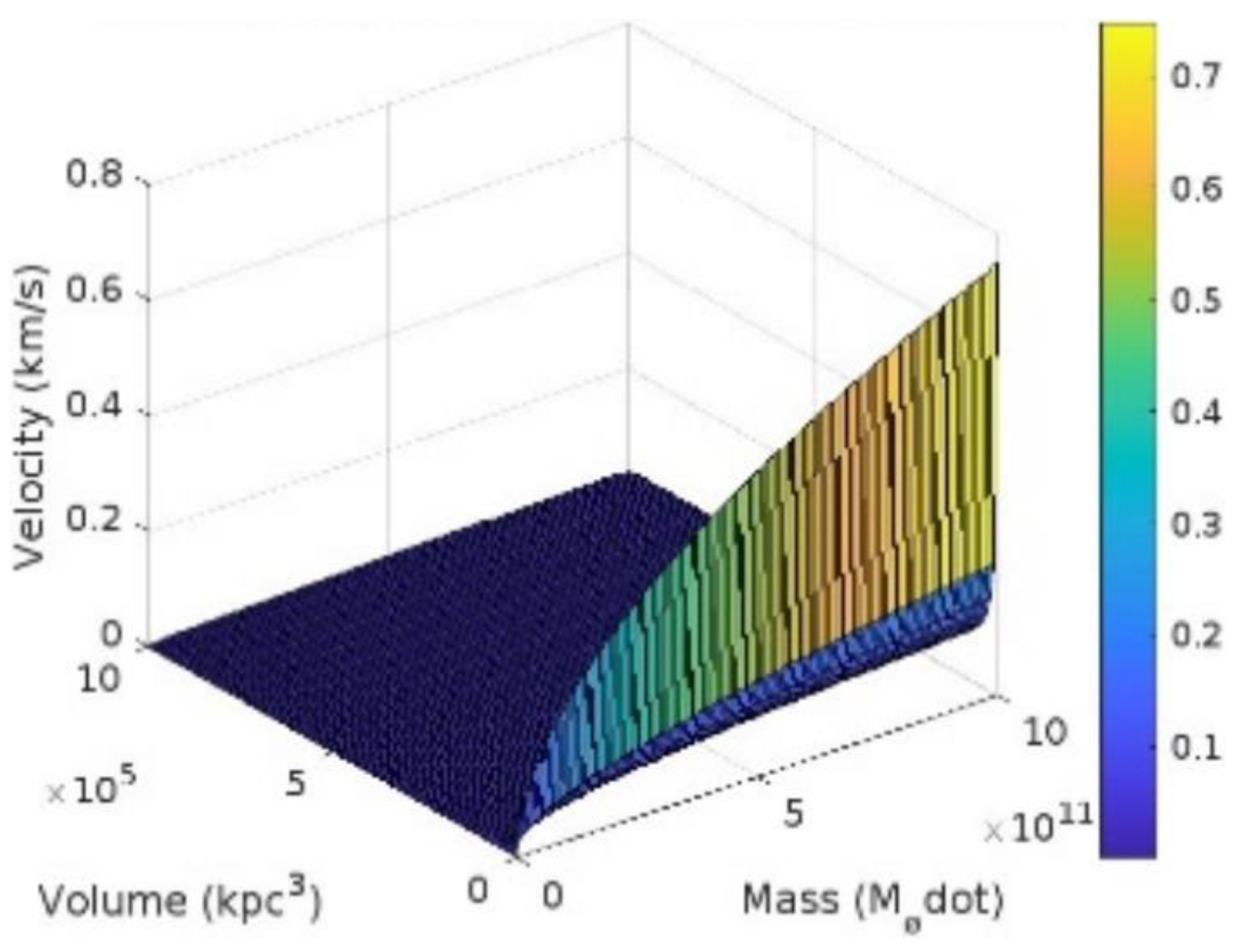
Figure 5.
Velocity as a Function of Mass and Volume. The figure (b) illustrates a three-dimensional surface plot that depicts the covariance between []AUE (Hubble Density) and the volume parameter (V 0) and (V 0 + 1). The ]AUE (Hubble Density) is displayed along the vertical axis and is observed to vary as a function of these two parameters. The color gradient, transitioning from blue to yellow, signifies the range of []AUE (Hubble Density) values, with blue representing lower densities and yellow indicating higher densities. The plot shows that as (V 0) and (V 0 + 1) increases, the ]AUE (Hubble Density) initially experiences a rapid increase before stabilizing, ultimately forming a plateau at elevated volumes. This behavior suggests a potential asymptotic covariance where ]AUE approaches a maximum limit in response to increasing volume parameters. The curvature of the surface indicates a change in the rate of variation of []AUE , which may reflect differing physical properties or dynamics associated with the expansion of the universe at various volume scales.
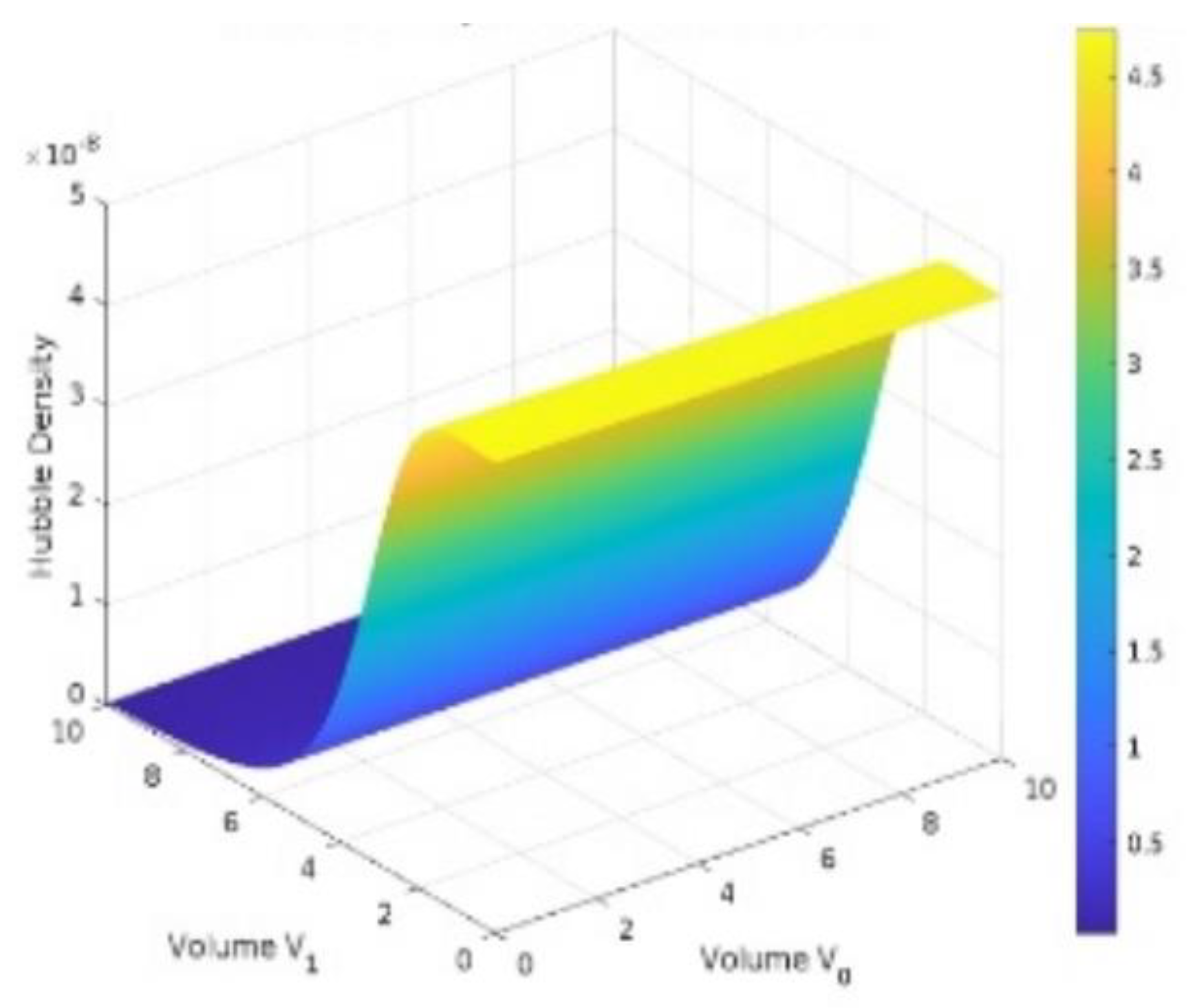
Figure 6.
Velocity,Mass,and Volume expansion. This 3D surface graph effectively illustrates the relationship between velocity (V), mass (in solar masses, M), and volume (in cubic kilo-parsecs, kpc³). The plot demonstrates how velocity varies across a defined grid of mass and volume values, with the colour gradient providing a clear visual representation of differing velocity magnitudes. The accompanying colour bar on the right indicates velocity in kilometers per second (km/s), where darker shades signify lower values and brighter shades represent higher values. This graph is a valuable tool for comprehending the interactions between cosmological mass and volume parameters within the framework of research focused on universal dynamics.
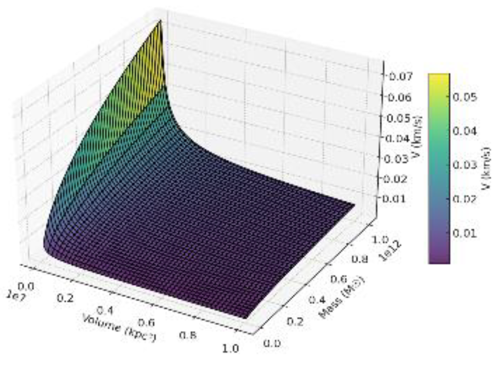
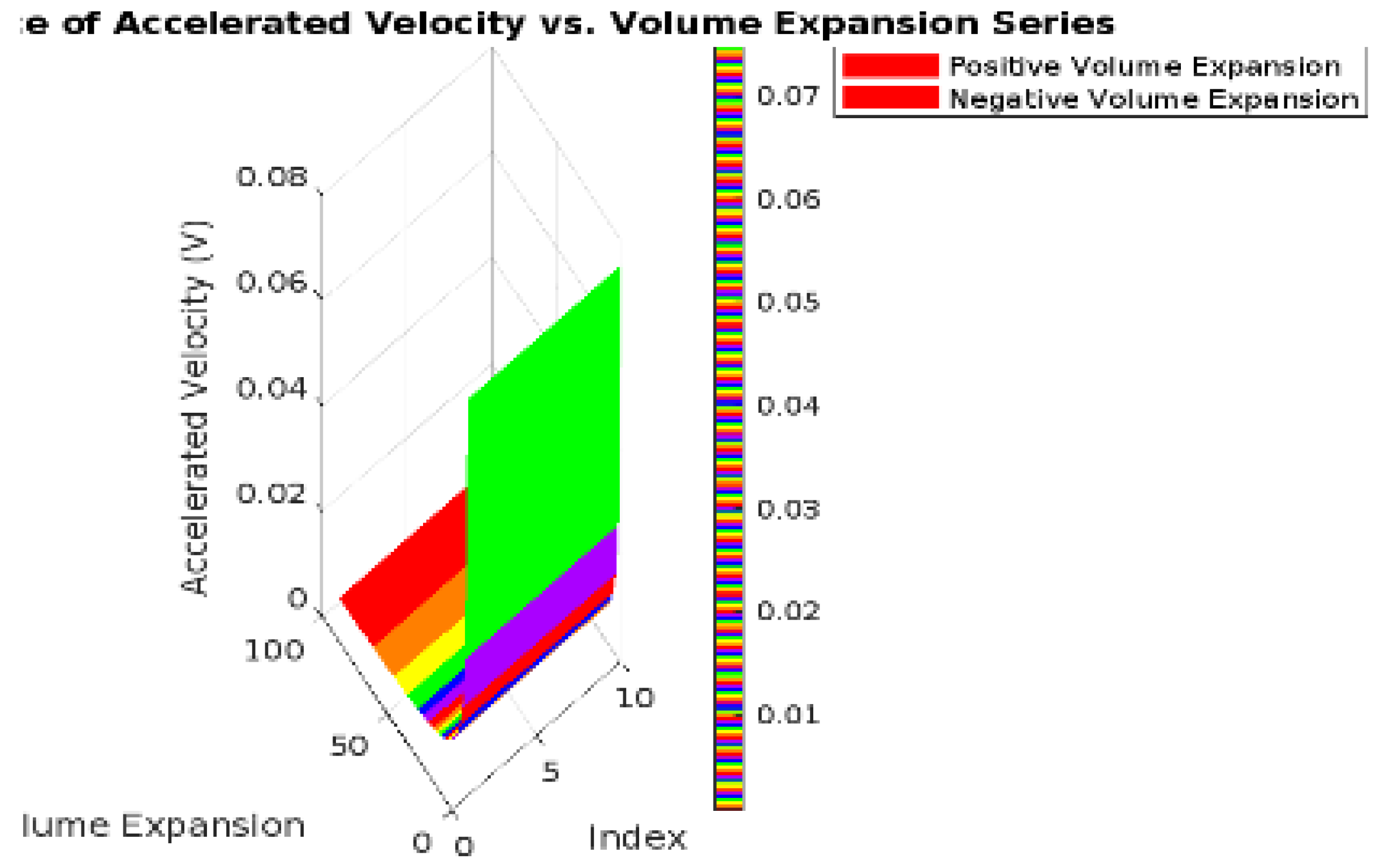
Figure 7.
Accelerated Velocity vs. Volume Expansion Series. The graph entitled "Graph of Accelerated Velocity vs. Volume Expansion Series" presents the relationship between accelerated velocity, depicted on the Y-axis, and the volume expansion index, illustrated on the X-axis. The data reveals two distinct trends. In the positive volume expansion region, there is an observable upward trend, indicating that as the volume expansion index increases, the accelerated velocity also rises, suggesting a direct or proportional relationship. In contrast, within the negative volume expansion region, the data shows a downward trend, reflecting a decline in accelerated velocity as the volume expansion index decreases, indicating an inverse relationship. This comprehensive graph effectively highlights the critical dynamics between velocity and volume changes, potentially serving a scientific or analytical purpose.
2. Conclusions
In this theory, calculate the relationship between the BCP and DCP ranges and the []AUE . This theory's recommendation sets that utilizing a particular methodology to calculate CHP, this theory indicate that a higher CHP correlates with lower overall compactness in an accelerated universe, which theory allude to as a “continual” [CHP. However, the existing challenges associated with the BCP and DCP and Hubble tension constrain this shift.
This theory posits that there exists a particular working parameters that in a perfect field serves to minimize the proposition of extra obscure parameters. This theory analysis encompasses a comprehensive exploration of all conceivable mechanism by which the universe accelerates at an elevate pace. Theory utilizes an expression that epitomizes this concept, including a grouping of term and that work as free variables parameter.
There are inalienable parameters within data or red-shift impacts that influence some of the result. Specifically, red-sift pertains to the methods utilize to degree the DCP. A eminent thought is that the accelerating expansion of the universe can affect the parameters to measure over different separate. Should the observed patterns not be attributable to the current parameters or specific effects, it prudent to consider alternative theories, such as modification to the Hubble equation, to crystallize the observations. The existing parameters do not appear to completely account for the drift in H0, theory proposing the plausibility new type of [CHP. This parameter could differ significantly for those outlined in the standard model. This phenomena indicates the need of study diametrical cosmological parameters to pick up a clear understanding of this unforeseen observation.
This concept sets that calculation [CHP offer valuable insights into addressing the current tension associated with BCP, DCP and []AUE matric. Whereas this approach showed up promising, it is essential to recognize that it cannot serves as a conclusive structure, Numerous perceptible and theoretical parameters necessitate ongoing exploration. This theory understanding of the interplay between the early and late universe acceleration remains incomplete. This theory building up these link could yield significant advancements in the development of new theoretical equation. This hypothesis continued research is critical to achieve a coherent interpretation of later infinite parameters, which ultimately deepen our understanding of the puzzling nature of the DCP and the accelerated expansion of the universe.
Author Contributions
Rizwan Ul Hassan developed the ideas. Rizwan also worked on creating equations, collecting data, and writing the code in MATLAB. He wrote the first draft of the paper. Anfal Fatima helped with formatting the paper, managing citations, and co-writing. Shahzaib edited the manuscript and fixed any mistakes. Umar Ashraf reviewed the manuscript. All authors have read and agreed on the final version of the paper.
Funding
This research received no external funding
Data Availability Statement
This theoretical theory does not use data from specific observations. Instead, the results are based on careful thinking and models created using current ideas about the universe. No outside data are used or designed for this research. If you would like more information about the calculations and results, you can ask the main author.
Acknowledgments
I want to say a big thank you to Dr Fayyaz Ahmad and Dr Irfan Toqeer for all their help and support while, I worked on this theory. Their advice and help were very important in developing this research and helped me better understand cosmic events.
Conflicts of Interest
The authors declare no conflicts of interest.
Appendix A. Mathematical Formulation of Universe Accelerate:
Volume Expansion Series:
Appendix B. Abbreviation
= Velocity of Universe Expansion(Red-Shift)
= 2.364624387 Distance of Expansion Universe
References
- Turner, M.S. The dark side of the universe: from Zwicky to accelerated expansion. Phys. Rep. 2000, 333, 619–635. [Google Scholar] [CrossRef]
- Krishnan, C. , et al., Sheikh-Jabbari and T. Yang. Phys. Rev. D 2020, 102, 2002.06044. [Google Scholar]
- Coles, P. and G.F.R. Ellis, Is the universe open or closed?: The density of matter in the universe. 1997: Cambridge University Press.
- Aloni, D.; Berlin, A.; Joseph, M.; Schmaltz, M.; Weiner, N. A Step in understanding the Hubble tension. Phys. Rev. D 2022, 105, 123516. [Google Scholar] [CrossRef]
- Di Valentino, E. , et al. In the realm of the Hubble tension—a review of solutions. Classical and Quantum Gravity 2021, 38, 153001. [Google Scholar] [CrossRef]
- Giarè, W. Inflation, the Hubble tension, and early dark energy: An alternative overview. Phys. Rev. D 2024, 109, 123545. [Google Scholar] [CrossRef]
- Niedermann, F.; Sloth, M.S. Resolving the Hubble tension with new early dark energy. Phys. Rev. D 2020, 102, 063527. [Google Scholar] [CrossRef]
- Tritton, D.J. Physical fluid dynamics. 2012: Springer Science & Business Media.
- Dainotti, M. , et al., The Hubble constant tension: current status and future perspectives through new cosmological probes. arXiv 2023, arXiv:2301.10572. [Google Scholar]
| 1 | Positive volume expansion parameters() |
| 2 | Negative volume expansion parameters() |
| 3 | Telescopic universe parameters |
| 4 | Dark universe parameters |
| 5 | Baryon Cosmological Parameter (Telescopic Universe) |
| 6 | Dark Cosmological Parameters (Lightless Universe) |
| 7 | Dark Physics Parameters |
| 8 | Critical density Parameter (Friedmann Equation) |
| 9 | Close Universe Parameters |
| 10 | Open Universe Parameters |
| 11 | Characterized as either a closed parameter indicating that it eventually curves back on itself or a flat parameter, suggesting that it extends infinitely without curvature. |
Disclaimer/Publisher’s Note: The statements, opinions and data contained in all publications are solely those of the individual author(s) and contributor(s) and not of MDPI and/or the editor(s). MDPI and/or the editor(s) disclaim responsibility for any injury to people or property resulting from any ideas, methods, instructions or products referred to in the content. |
© 2024 by the authors. Licensee MDPI, Basel, Switzerland. This article is an open access article distributed under the terms and conditions of the Creative Commons Attribution (CC BY) license (http://creativecommons.org/licenses/by/4.0/).
Copyright: This open access article is published under a Creative Commons CC BY 4.0 license, which permit the free download, distribution, and reuse, provided that the author and preprint are cited in any reuse.


