
Submitted:
26 November 2024
Posted:
27 November 2024
You are already at the latest version
Abstract
Domination problems are fundamental problems in graph theory with diverse applications in optimization, network design, and computational complexity. This paper investigates {k}-domination, k-tuple domination, and their total domination variants in weighted strongly chordal graphs and chordal bipartite graphs—two well-studied subclasses of chordal graphs and bipartite graphs. We extend existing theoretical models to explore the less-explored domain of vertex-weighted graphs and establish efficient algorithms for these domination problems. Specifically, the {k}-domination problem in weighted strongly chordal graphs and the total {k}-domination problem in weighted chordal bipartite graphs are shown to be solvable in O(n+m) time. For weighted proper interval graphs and convex bipartite graphs, we solve the k-tuple domination and total k-tuple domination problems in O(n^{2.371552}log^{2}(n)log(n/δ)), where δ is the desired accuracy. Furthermore, for weighted unit interval graphs, the k-tuple domination problem achieves a significant complexity improvement, reduced from O(n^{k+2}) to O(n^{2.371552}log^{2}(n)log(n/δ)). These results are achieved through a combination of linear and integer programming techniques, complemented by totally balanced matrices, totally unimodular matrices, and graph-specific matrix representations such as neighborhood and closed neighborhood matrices.
Keywords:
domination
; total domination
; {k}-domination
; k-tuple domination
; strongly chordal graph
; chordal bipapartite graph
; proper interval graph
; convex bipartite graph
; totally balanced matrix
; totally unimodular matrix
1. Introduction
Domination is a fundamental concept in graph theory and widely regarded as a critical graph optimization problem. Over the years, it has attracted significant attention due to its diverse applications in network design, resource optimization, social network analysis, and computational complexity. Its importance was first notably recognized in 1990, when a special issue of Discrete Mathematics was dedicated entirely to this topic [1]. By 1998, more than 1,200 papers had been published on domination and its variants, which led to the release of two seminal books on the subject [2,3]. Since then, the field has experienced rapid growth, with over 5,000 papers exploring various types of domination in graphs. Three additional books [4,5,6] have been published in recent years to capture the latest advancements in domination theory. Among these variants, total domination has gained particular prominence and has become a well-researched problem, as outlined in [7].
1.1. Current Research Directions
An active area of current research focuses on -domination and total -domination. Domination and total domination are special cases when . Extensive studies on these problems have revealed insights into computational complexity and solution techniques [8,9,10,11,15,20,21,22,23,24,25,26,27,28,29,30,31,32,33]. For instance, -domination is polynomial-time solvable for strongly chordal graphs, but remains NP-complete for chordal bipartite graphs [8]. Similarly, total -domination is solvable in polynomial time for chordal bipartite graphs [9] but NP-complete for bipartite planar graphs [10]. From an approximation perspective, both problems can be approximated within a factor of in polynomial time, where n is the number of vertices in the graph [11].
Beyond -domination, the k-tuple domination and total k-tuple domination problems have also garnered attention. While polynomial-time solutions exist for specific graph families, such as strongly chordal graphs, interval graphs, and web graphs [12,13,14], the problems remain NP-complete for others, such as chordal and planar graphs [12,15]. The k-tuple total domination problem can be solved in time for weighed proper interval graphs [16]. Furthermore, for , the running time of can be improved to be . For weighted unit interval graphs, the k-tuple and total k-tuple domination problems can be solved in and time [17], respectively. The dichotomy between tractable and intractable cases has also been a focus of study in [36,37,38,39,40,41,42,43].
1.2. Research Gap and Motivation
Despite significant advancements, most studies on (total) -domination and (total) k-tuple domination have concentrated on unweighted graphs. Comparatively, much less attention has been given to these problems in weighted graphs, despite their widespread use in real-world systems to model costs, capacities, or priorities. Exploring these domination problems in weighted graphs offers a significant opportunity for further research and development.
To bridge this gap, we focus on the -domination and total -tuple domination problems for weighted strongly chordal graphs and chordal bipartite graphs. Additionally, we investigate k-tuple domination and total k-tuple domination for weighted proper interval graphs and weighted convex bipartite graphs.
1.3. Scope of Study
Strongly chordal graphs and chordal bipartite graphs are well-studied classes that include several important subclasses, such as trees, proper interval graphs, convex bipartite graphs, and bipartite permutation graphs [18]. These classes are characterized by specific vertex ordering constraints, which facilitate various computational operations. Employing these properties, we aim to develop efficient algorithms for solving domination problems on weighted graphs.
Most existing research on domination in weighted graphs assigns weights to vertices, with each vertex’s weight representing attributes like importance, cost, or influence that directly impact domination parameters. Following this convention, this paper focuses exclusively on vertex-weighted graphs, and the term “weighted graph” refers specifically to this context.
1.4. Contributions
This paper presents the following contributions:
- -Domination for Weighted Strongly Chordal Graphs: We demonstrate that the -domination problem in weighted strongly chordal graphs can be solved in time, where n and m denote the number of vertices and edges, respectively. This result is achieved by refining Hoffman et al.’s method [19] and leveraging properties of adjacency lists and totally balanced matrices.
- Total -Domination for Weighted Chordal Bipartite Graphs: Building on structural similarities between chordal bipartite graphs and strongly chordal graphs, we extend the refined framework to solve the total -domination problem in time for weighted chordal bipartite graphs.
- -Tuple Domination for Weighted Proper Interval Graphs: Using linear and integer linear programming techniques, we solve the k-tuple domination problem for weighted proper interval graphs in time, where is the desired accuracy. Since a graph is a proper interval graph if and only if it is a unit interval graph [18], we reduce the complexity from [17] to
- Total -Tuple Domination for Weighted Convex Bipartite Graphs: We achieve the same time complexity bound, , for solving the total k-tuple domination problem in weighted convex bipartite graphs.
This study is purely theoretical and includes formal proofs of correctness and efficiency, enriching the understanding of domination problems in these graph classes.
1.5. Organization of the Paper
The remainder of the paper is organized as follows:
-
Section 2: PreliminariesThis section provides a foundation of essential concepts and definitions that underpin our research. We introduce and explore fundamental properties of strongly chordal graphs, chordal bipartite graphs, proper interval graphs, and convex bipartite graphs. To set the stage for our linear programming approach, we formally define (total) -domination and (total) k-tuple domination. Additionally, we review matrix-theoretic tools, specifically adjacency matrices, totally balanced matrices, greedy matrices, and totally unimodular matrices, which play a critical role in our modeling framework.
-
Section 3: -Domination in Weighted Strongly Chordal GraphsThis section formulates the -domination problem an integer linear program in matrix form. We demonstrate how to solve the -domination problem for weighted strongly chordal graphs in time by refining Hoffman et al.’s method [19] using concepts from totally balanced matrices, greedy matrices, and adjacency lists.
-
Section 4: Total -Domination in Weighted Chordal Bipartite GraphsThis section describes how to adapt the matrix-based framework to solve the total -domination problem in weighted chordal bipartite graphs. By using the structural similarities between chordal bipartite and strongly chordal graphs, we demonstrate the versatility of our approach and provide a comprehensive analysis of its applicability to both graph types.
-
Section 5: -Tuple Domination and Total -Tuple DominationThis section focuses on using linear and integer linear programming for totally unimodular matrices to solve the k-tuple domination problem for weighted proper interval graphs and the total k-tuple domination problem for weighted convex bipartite graphs in time.
-
Section 6: ConclusionsThe paper concludes by summarizing our findings, discussing the theoretical implications of our results, and proposing directions for future research that extends these domination techniques to other classes of weighted graphs.
2. Preliminaries
This paper integrates critical insights from multiple fields, including graph classes, linear algebra, graph theory, algorithms, and linear programming, each contributing indispensable tools and perspectives that enhance both the formulation and depth of our analysis. This section presents the fundamental concepts most pertinent to understanding the study’s objectives and methodology. For definitions, notations, additional concepts, or more comprehensive details not covered in this section, standard textbooks and monographs—such as Introduction to Algorithms [44], Theory of Linear and Integer Programming [45], Graph Theory [46], Introduction to Linear Algebra [47], and Graph Class: A Survey [18]—are recommended as supplementary resources.
2.1. Graphs and Their Representations
Each graph in this paper is finite, undirected, and contains no multiple edges or self-loops, where V is the vertex set and E is the edge set of G. If the vertex and edge sets are not explicitly specified, they are denoted by and , respectively.
Two vertices u and v in a graph G are adjacent if they are connected with an edge, i.e., , and are also called neighbors. The degree of a vertex v in G, denoted by , is the number of neighbors of v. For any vertex , the neighborhood of v in G, denoted by , is the set of neighbors of v, so that . A vertex u is a closed neighbor of v if either or . The closed neighborhood of v, denoted by , is the set of closed neighbors of v.
Let and be two graphs. If and , then is a subgraph of G. If is a subraph of G, and contains all the edge with , then is an induced subgraph; we say that is induced by and written as .
Graphs in this paper are represented using adjacency lists. The adjacency-list representation of a graph consists of an array of lists. Each vertex is associated with a list of all neighbors of v. Figure 1 provides an example of the adjacency-list representation for a graph G with 4 vertices and 4 edges.
This representation is efficient in terms of memory usage. The amount of memory required to store a graph in this representation is , where n and m represent the number of vertices and edges, respectively. Adjacency lists support efficient operations such as
- Neighbor Access: Accessing all (closed) neighbors of a vertex v takes time, as they are directly stored in a list. With each vertex maintaining its own neighbor list, this structure enables quick access to both neighbors and closed neighbors.
- Traversal: Traversing all vertices and edges in the graph takes time. This efficiency is particularly advantageous in algorithms like Depth-First Search (DFS) and Breadth-First Search (BFS).
2.2. -Domination and Total -Domination in Weighted Graphs
A dominating set D of a graph is a subset of V such that for every , while a total dominating set D is a subset of V such that for every . The domination number of G, denoted by , is the minimum cardinality of a dominating set of G. The total domination number of G, denoted by , is the minimum cardinality of a total dominating set of G. The domination problem is to find a dominating set of G with the minimum cardinality, and the total domination problem is to find a total dominating set of G with the minimum cardinality.
Figure 2 illustrates a dominating set and a total dominating set for the same graph. Let G denote the graph in this figure. While also qualifies as a dominating set of G, does not qualify as a total dominating set, since is empty for .
Domination and total domination can be expressed in terms of functions. Let be a labeling function of a graph . The function f is a dominating (respectively, total dominating) function of G if (respectively, ) for every . The labeling weight of f is defined as .
Table 1 presents a dominating function f and a total dominating function g for the graph shown in Figure 2. The function f is associated with the set and g with the set . Both functions have a labeling weight of 2, equal to and , respectively.
Clearly, the domination number is the minimum labeling weight of a dominating function, i.e.,
Similarly, the total domination number is the minimum labeling weight of a total dominating function, i.e.,
Definition 1.
Let k be a fixed positive integer, and let be a labeling function of a graph . The function f is a -dominating (respectively, total -dominating) function of G if (respectively, ) for every . The labeling weight of f is defined as . The -domination problem is to find a -dominating function of G with the minimum labeling weight, while the total -domination problem is to find a total -dominating function of G with the minimum labeling weight.
By Definition 1, domination and total domination correspond to -domination and total -domination, respectively.
Let G be the graph shown in Figure 2. Table 2 provides the values of a function f for each vertex in G and checks whether the -domination condition is satisfied. This verification confirms that f is a valid -dominating function for G.
We now introduce the concepts of -domination and total -domination for weighted graphs. As mentioned earlier in the introduction, this paper focuses exclusively on vertex-weighted graphs.
Definition 2.
Let be a function that assigns a weight to each vertex v of a graph . We refer to w as a vertex-weight function, and as a weighted graph.
Definition 3.
Let k be a fixed positive integer. The labeling weight of a -dominating function or a total -dominating function f of a weighted graph is defined as . The -domination problem for a weighted graph is to find a -dominating function of G with the minimum labeling weight, while the total -domination problem is to find a total -dominating function with the minimum labeling weight.
An unweighted graph H can be treated as a specific case of a weighted graph, where every vertex has a weight . The primary difference in defining the -domination problem for unweighted and weighted graphs lies in the calculation of the labeling weight.
- In unweighted graphs, the labeling weight of a -dominating function is simply the sum of the function values assigned to each vertex, i.e., , where each vertex has an implicit weight of 1.
- In weighted graphs, each vertex is assigned a specific weight through a vertex-weight function. The labeling weight is then calculated as , meaning that the contribution of each vertex to the total weight depends on both the value of the labeling function and the vertex’s weight .
Table 3 presents the values of a -dominating function f and vertex weights w for the graph shown in Figure 2. The table indicates that the labeling weight of f for the unweighted graph G is 4, based on , and the labeling weight for the weighted graph is 12, calculated as .
This distinction also applies to the definitions of total -domination on unweighted and weighted graphs. Therefore, the introduction of vertex weights in weighted graphs alters how the overall labeling weight is determined in both the -domination and total -domination problems.
2.3. k-Tuple Domination and Total k-Tuple Domination in Weighted Graphs
Let k be a fixed positive integer, and let be a labeling function for a graph . The function f is a k-tuple dominating function of G if for every . Similarly, f is a total k-tuple dominating function if for every . The labeling weight of f is defined as .
The k-tuple domination problem aims to find a k-tuple dominating function of G with the minimum labeling weight. Similarly, the total k-tuple domination problem seeks a total k-tuple dominating function with the minimum labeling weight.
Domination and total domination correspond to 1-tuple domination and total 1-tuple domination, respectively.
Definition 4.
Let k be a fixed positive integer. The labeling weight of a k-tuple dominating function or a total k-tuple dominating function f of a weighted graph is defined as . The k-tuple domination problem for a weighted graph is to find a k-tuple dominating function with the minimum labeling weight. Similarly, the total k-tuple domination problem is to find a total k-tuple dominating function with the minimum labeling weight.
Figure 3 illustrates a graph with six vertices. Table 4 provides the labeling weights for a 2-tuple dominating function f and a total 2-tuple dominating function g for both the unweighted graph G and the weighted graph .
The function f assigns values as shown in the table, satisfying the 2-tuple domination condition for each vertex. For instance, vertex is dominated because . The labeling weights differ for the unweighted and weighted versions due to the vertex weights .
Interestingly , g is also a 2-tuple dominating function of G. However, for the weighted graph , the labeling weight of g is smaller than that of f, demonstrating that g is more efficient in terms of weight minimization.
2.4. Strongly Chordal Graphs and Chordal Bipartite Graphs
A chord in a cycle of a graph is an edge that connects two non-consecutive vertices in the cycle. A chordal graph is a graph in which every cycle with four or more vertices has a chord. A perfect elimination ordering of a graph is an ordering of the vertices such that for any indices , if and , then . Rose [48] proved that a graph is chordal if and only if it admits a perfect elimination ordering.
A chord in a cycle C with vertices ordered as is called an odd chord if is odd. A graph G is a strongly chordal graph if it is chordal, and every cycle of vertices in G, where , contains an odd chord. Figure 4 demonstrates a strongly chordal graph and the Hajós graph. The Hajós graph is chordal but not strongly chordal since the cycle contains no odd chords.
A strong elimination ordering of a graph is a perfect elimination ordering such that for each and , if , , and , then . Farber [49] proved that a graph is strongly chordal if and only if it admits a strong elimination ordering. Figure 4 shows a strongly chordal graph with a strong elimination ordering .
A bipartite graph is a graph in which the vertex set can be partitioned into two disjoint sets X and Y such that every edge in the graph connects a vertex in X to a vertex in Y, and no edge connects two vertices within the same set. In other words, there are no edges between vertices within X or within Y. Therefore, a bipartite graph does not have a cycle of an odd number of vertices. Figure 5 shows two graphs: The left one is bipartite, while the right one contains a cycle of three vertices and is therefore not bipartite.
A chordal bipartite graph is a bipartite graph in which every cycle of more than four vertices contains a chord. Figure 6 shows two bipartite graphs: The left one is chordal bipartite, while the right one is not.
Let be a graph, and let be an ordering of V. Let be a subgraph of G induced by . A weak elimination ordering of G is an ordering such that for any indices , if , then .
2.5. Proper Interval Graphs and Convex Bipartite Graphs
A graph is an interval graph if there exits an interval model on the real line such that each closed interval in the interval model corresponds to a vertex , and two vertices are adjacent in G if and only if their corresponding intervals overlap, that is:
Figure 7 illustrates an interval graph , which is constructed from an interval model on the real line. The top part of the figure represents the intervals , , , and , labeled as vertices and , respectively. An edge exists between two vertices if their corresponding intervals overlap. For example, the intervals and overlap, resulting in an edge between and in the graph. Similarly, and share an edge due to the overlap of their intervals, as do and .
The lower part of the figure depicts the corresponding graph structure. The vertices and are connected by edges according to their interval overlaps, forming a path graph. .
An interval graph is called a proper interval graph if there exists an interval model for this interval graph such that for every pair of intervals and in the model, neither interval is strictly contained within the other, i.e., it is not true that and . A unit interval graph is a special type of interval graph where all the intervals associated with the vertices have the same length. Actually, a unit interval graph G if and only if G is a proper interval graph [18]. They form the same class of graphs.
Let be a bipartite graph. An ordering P of X in B has the adjacency property if for each vertex , consists of vertices that are consecutive in the ordering P of X. A bipartite graph is a convex bipartite graph if there is an ordering of X or Y satisfying the adjacency property.
The convex bipartite graph illustrated in Figure 8 consists of two disjoint sets of vertices, and . The graph satisfies the adjacency property: for every vertex in U, the vertices of its neighbors in V are consecutive in the ordering. For instance, the neighbors of are and are consective in the ordering. Similarly, is adjacent to consecutive vertices , , and . This property is consistent for all vertices in U.
2.6. Matrices and Vectors
A matrix is a rectangular array of numbers arranged in rows and columns. The horizontal arrangement of entries forms the rows, and the vertical arrangement forms the columns. An matrix is a matrix with m rows and n columns. The individual numbers within the matrix are called entries. The entry in the i-th row and j-th column is called the -entry.
Matrices are typically written within square brackets or parentheses; in this paper, they are written within parentheses. For example, a matrix is written as
Let represent the entry in the i-th row and j-th column of an matrix . The matrix can be denoted by and represented as follows:
where represents the set of all matrices with m rows and n columns whose entries are real numbers. Formally, this is defined as
For any matrices and in , we define the entrywise inequality to mean that for all and . For any scalar , we write to indicate that every entry of is at least k. These definitions extend naturally to other similar cases involving entrywise comparisons. If each entry of is k, then is called a k-matrix.
Let . The transpose of A, denoted by , is an matrix defined by . For a matrix
which is a matrix, its transpose is
which is a matrix.
A submatrix of a matrix is obtained by removing any number of rows or columns from , including the possibility of removing none. Consequently, is a submatrix of itself when no rows or columns are removed.
A block of matrix is a submatrix formed by rows and columns . It is represented as:
where and . The following matrix consists of four blocks , , , and :
A square matrix is a matrix with the same number of rows and columns. The identity matrix is a square matrix such that an entry of is 1 if its row index and column index are equal; otherwise, . For example, the identity matrix looks like this:
A row vector and a column vector are two types of vectors that differ in their orientation within a matrix or vector space. A row vector is a matrix represented as
where are the vector elements. A column vector is an matrix represented as
where are the vector elements. Clearly, the transpose operation converts a row vector into a column vector and vice versa.
To ensure clarity and avoid ambiguity in notation, we adopt the following conventions: Vectors are represented by boldface upright lowercase letters, such as , , or . For example, denotes a column vector with n entries. Matrices are represented by boldface upright uppercase letters, such as , , or , and entries of a matrix are denoted by for the entry in the i-th row and j-th column. Scalars, by contrast, are represented by italicized lowercase letters, such as a, b, or c.
In general, when we refer to as a vector, we mean that it is a column vector by default. If a row vector is intended, this will be explicitly indicated. If each entry of a vector is a constant k, the vector is called a k-vector.
2.7. Totally Balanced, Totally Unimodular, and Greedy Matrices
A matrix is called a -matrix if every entry in is either 1 or 0. In a matrix of numbers, the sum of all entries in a row is called the row sum, while the sum of all entries in a column is called the column sum. A -matrix is said to be totally balanced if it does not contain any square submatrix satisfying all the following “forbidden conditions”:
- All row sums are equal to 2.
- All column sums are equal to 2.
- All columns are distinct.
Here is an example of a matrix that is not totally balanced:
To see why is not totally balanced, consider the the submatrix obtained by removing the 4th and 5th rows and columns:
In , (1) all row sums are equal to 2, (2) all column sums are equal to 2, and (3) all columns are distinct. This submatrix satisfies the forbidden conditions, so is not totally balanced. In contrast, the following matrix is an example of a totally balanced matrix:
A -matrix is greedy if it does not contain any of the following forbidden submatrices:
A greedy matrix is in standard greedy form [19] if it does not contain the following -matrix as a submatrix:
The matrix below is a greedy matrix in standard greedy form. However, the matrix is a greedy matrix that is not in standard greedy form. This is because the submatrix of formed by deleting rows 3 and 4 and columns 3 and 4 is identical to the -matrix.
Let denote the determinant of a matrix . The matrix M is totally unimodular if for every square submatrix of .
Consider the matrices and :
The matrices and illustrate examples of a totally unimodular matrix and a matrix that is not totally unimodular, respectively. Matrix is totally unimodular because the determinant of every square submatrix of is in . In contrast, matrix is not totally unimodular. For example, is 2. Thus, fails to satisfy the defining condition of total unimodularity. This comparison underscores the stringent conditions a matrix must satisfy to be classified as totally unimodular.
Furthermore, a matrix has the consecutive ones property if its rows can be permuted in such a way that, in every column, all the 1s appear consecutively. This property is particularly relevant in applications involving binary matrices and is a useful tool for analyzing matrix structures.
The following theorem reveals a connection between the consecutive ones property and total unimodularity.
Theorem 1
([45]). If a -matrix has the consecutive ones property for columns, then it is totally unimodular.
2.8. Linear and Integer Linear Programming
Linear programs are optimization problems that maximize or minimize a linear objective function, subject to linear constraints. A minimization linear program seeks to minimize the objective function, while a maximization linear program aims to maximize it.
Linear programming is the field of study and methodology focused on formulating, analyzing, and solving linear programs. It encompasses the theories, algorithms, and techniques developed for solving linear programs. In essence, linear programming refers to the process and theory, while a linear program is an individual problem instance.
Formulating a minimize linear program requires the following inputs: n real numbers (coefficients of the objective function), m real numbers (resource limits), and coefficients for and (constraint coefficients). The goal is to find values for the decision variables that minimize the objective function, subject to all constraints. This formulation is given by:
In this formulation, the expression in (1) is the objective function; the variables , are called decision variables; and the inequalities in () and () together form the constraints. Specifically, the n inequalities in () are nonnegativity constraints, requiring each to be nonnegative.
In mathematical optimization, duality provides two perspectives on an optimization problem: the primal problem and its corresponding dual. When the primal is a minimization problem, its dual is a maximization problem, and conversely, when the primal is a maximization problem, the dual will be a minimization problem. Thus, for a pair of primal and dual problems, one is a maximization problem, and the other is a minimization problem.
Weak duality states that, for any feasible solutions to a pair of primal and dual problems, the value of the maximization problem is always less than or equal to the value of the minimization problem. Strong duality further asserts that, at optimality, the optimal value of the primal problem is equal to the optimal value of its dual.
For any linear program considered as the primal, there exists a corresponding dual linear program. Each constraint in the primal corresponds to a variable in the dual, and each decision variable in the primal corresponds to a constraint in the dual. The dual of the minimization linear program in equations 1– is formulated as follows:
In this dual problem, are the dual variables associated with each primal constraint; are the coefficients of the dual objective function; and constraints in the dual correspond to the primal variables, and values become the bounds in the dual constraints.
For a minimization linear problem, the primal can be written in matrix form as
where , , , and . Its dual can be expressed as
where, ; , , and are as defined in the primal formulation.
In many cases, capturing the essence of a linear program is best achieved without excessive notation or detail. To highlight the fundamental structure clearly and concisely, we adopt forms such as
to facilitate analysis, communication, and efficient solution of linear programs.
A solution to an optimization problem is a column vector , often called a point because each solution corresponds to a specific set of values for the variables, which can be represented as a single point in geometric space. In other words, each feasible solution is associated with a unique location in this space. A solution that satisfies all constraints is known as a feasible solution, whereas a solution that fails to satisfy at least one constraint is an infeasible solution. The set of points that satisfy all the constraints is referred to as the feasible region. In linear programming, the feasible region is called a polyhedron, as it is the intersection of linear constraints. A polyhedron is often denoted by P, such as , representing the set of all points that meet the specified constraints.
In an optimization problem, a constraint is called active at a given solution point if the solution causes the constraint to hold as an equality, effectively “binding” the solution at the boundary defined by the constraint. An extreme point of a polyhedron occurs where several of the constraints in the problem are active, often as many as the dimension of the space.
The fundamental theorem of linear programming ([51]) states that if a linear program has an optimal solution, at least one optimal solution will be located at an extreme point of the polyhedron. This result is foundational because it allows optimization algorithms like the simplex method to focus on the extreme points of the feasible region, significantly reducing the computational effort required to find an optimal solution. If every extreme point of a polyhedron consists of integer values for all variables, then the polyhedron is said to be integral.
Theorem 2 establishes that linear programs satisfy strong duality.
Theorem 2
An integer linear program is an optimization model similar to a linear program but includes an additional constraint that requires all decision variables to be integers. This distinction substantially impacts both the complexity and solution methods for these problems. While linear programs can be solved in polynomial time [52], integer linear programs are NP-complete [53], making them more computationally challenging.
Integer linear programs satisfy weak duality but do not always satisfy strong duality, meaning the optimal values of an integer linear program and its dual may differ.
To solve integer linear programs, advanced methods such as branch-and-bound, branch-and-cut, and cutting planes are often employed. These methods frequently use linear relaxations, which remove the integer constraints to produce a continuous solution, providing useful bounds on the solution to an integer linear program. In certain cases, the optimal objective value of an integer linear program matches that of its linear relaxation, as illustrated by Theorem 3.
Theorem 3
([54]). If , , and all have integer entries, with at least one of or as a constant vector, and is totally balanced, then the optimal objective values of the integer program
and its linear relaxation are the same.
3. -Domination in Weighted Strongly Chordal Graphs
In this section, we demonstrate that the -domination problem in weighted strongly chordal graphs with n vertices and m edges can be solved in time. The solution follows a four-step framework, as outlined below:
- (1)
- Modeling (Section 3.1): The -domination problem is formulated as an integer linear programming task using matrix representations, particularly adjacency matrices. This formulation establishes the theoretical foundation for the algorithmic approaches described in subsequent sections. We aim to solve the integer linear program by its relaxation.
- (2)
-
Primal and Dual Algorithms by Hoffman et al. (Section 3.2): We introduce the primal and dual algorithms proposed by Hoffman et al. [19], which solve the linear program:These algorithms provide a robust framework for solving linear programming problems, forming the basis for adapting solutions to the -domination problem.
- (3)
- Refined Algorithms for Weighted Strongly Chordal Graphs (Section 3.3): Building on Hoffman et al.’s algorithms, this section introduces refinements tailored to the structural properties of weighted strongly chordal graphs. These refinements reduce the computational complexity to , representing an intermediate step toward the final optimized solution.
- (4)
- Optimized Algorithms with Enhanced Data Structures (Section 3.4): By integrating advanced data structures, this section further reduces the overall time complexity from to . This optimization capitalizes on the sparsity and adjacency structure of strongly chordal graphs, achieving linear-time performance relative to the graph’s size.
3.1. Modeling
We start by presenting Lemma 1 to concentrate exclusively on non-negative vertex weights (). This simplification allows us to assume that all weighted graphs have non-negative vertex weights.
Lemma 1.
Let w be a vertex-weight function of a graph , and let represent the the minimum labeling weight of a -dominating function for . Define and let be a vertex-weight function such that for each . Then, .
Proof.
Let f be a -dominating function for with minimum weight, so . Define a function such that for and for . Since is also a -dominating function of G and for , we obtain
Conversely, let h be a -dominating function for with the minimum labeling weight, so
Define f such that for and for . Clearly, f is a -dominating function of G, and for . We have
This completes the proof. □
Let be a weighted graph with . We associate a variable with each and require that for . Let for . The -domination problem for the weighted graph G is formulated as the following integer linear program :
Lemma 2.
Let be an optimal solution to . Then, for all .
Proof.
Clearly, is the minimized and for . Assume that there exists an in such that . For any constraint involving , the constraint remains satisfied if is replaced with k. Consequently, the resulting objective value is less than , leading to a contradiction. Therefore, the lemma holds. □
By Lemma 2, we can reformulate as follows:
In graph theory, the neighborhood matrix and the closed neighborhood matrix are two distinct representations of the adjacency relationships in a graph H with vertices .
- The neighborhood matrix of G is a matrix such that if ; otherwise, .
- The closed neighborhood matrix of G is a matrix such that if ; otherwise, .
Let be the closed neighborhood matrix of the weighted graph G with , , and , where for .
We present the linear program and its dual using the closed neighborhood matrix .
Let and denote the optimal objective values of an integer linear program and its linear relaxation , respectively. The polyhedron for is a subset of the polyhedron for , since includes the additional constraint that variables must be integers. Therefore, the optimal value of , minimized over a larger polyhedron, cannot be greater the optimal value of . Hence, .
In subsequent sections, we aim to demonstrate that for weighted strongly chordal graphs, the optimal value of is equal to the optimal value of its linear relaxation . This allows us to solve this integer linear program by obtaining an integral solution directly from its linear relaxation.
3.2. Primal and Dual Algorithms by Hoffman et al.
Let be a greedy matrix in standard form, with vectors , , and as variables. Let , , and be constant vectors with , , and . The primal linear program P is defined as:
The dual program D is formulated as:
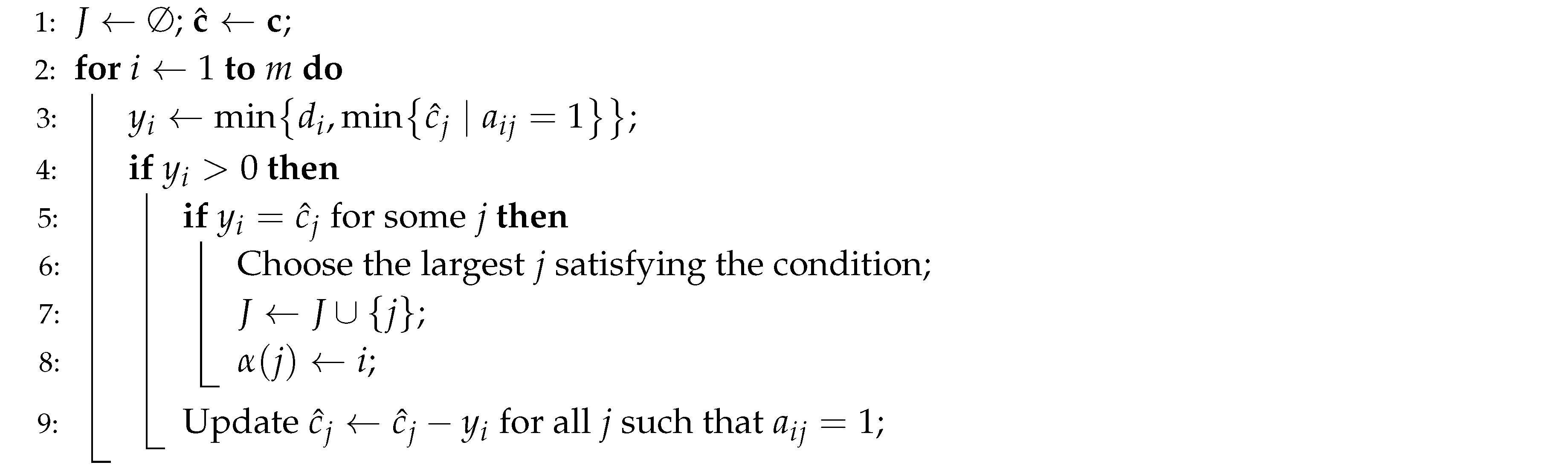
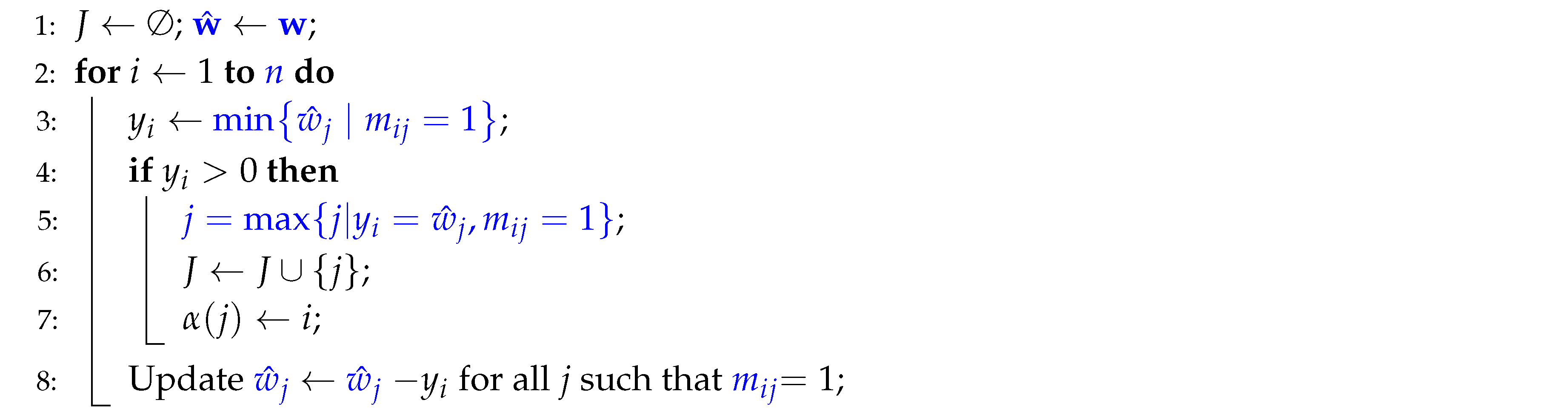
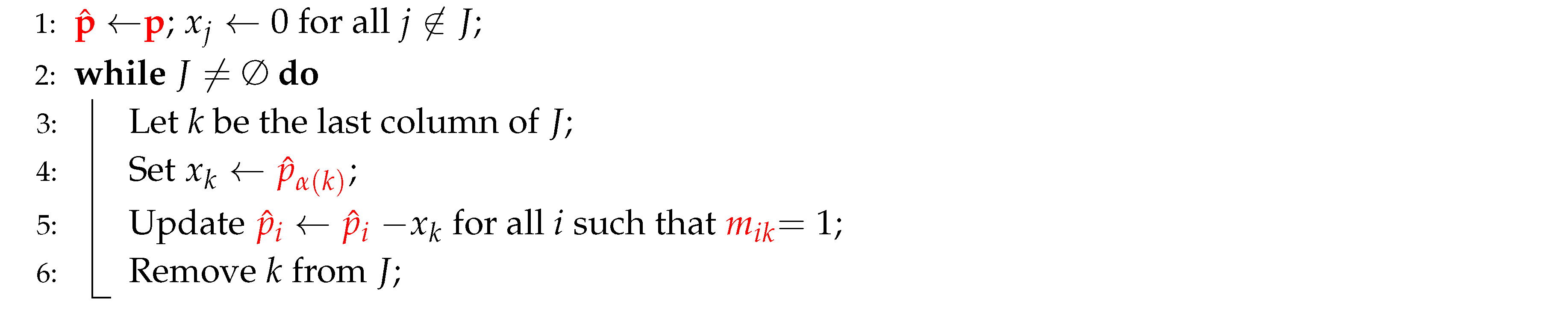
Hoffman et al. [19] introduced two greedy algorithms to solve P and its dual D in polynomial time, and constructed an integer optimal solution for P. These algorithms are presented in Algorithms 1 and 2.
Algorithm 1 provides an integer optimal solution for D. The dual program D contains n constraints and m decision variables . A constraint j is defined as tight if
Let and . Algorithm 1 determines each variable in increasing order of i and takes the largest feasible value. It also computes J and for use in Algorithm 2.
| Algorithm 1: Dual Solution for Program D with Greedy Matrices |
 |
Algorithm 2 computes the primal solution corresponding to the dual solution by iteratively adjusting values.
| Algorithm 2: Primal Solution for Program P Corresponding to Dual Solution |
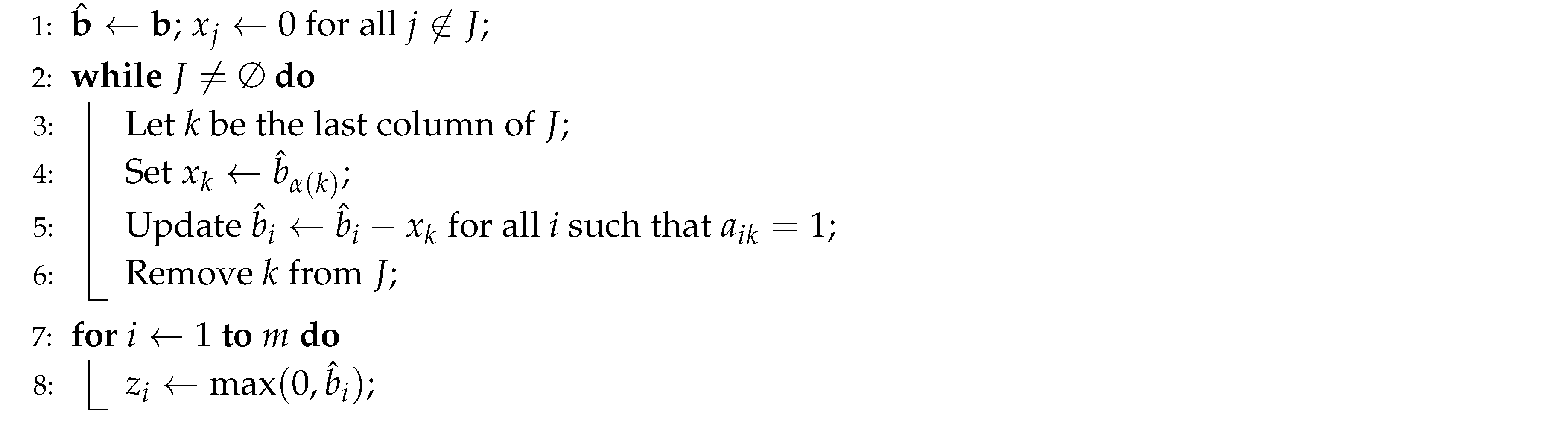 |
Theorem 4
( [19]). The dual program D is solved by Algorithm 1 for all , and if and only if A is greedy in standard greedy form. Further, Algorithm 2 constructs an integer optimal solution to the primal problem P. Both algorithms run in time.
3.3. Refined Algorithms for Weighted Strongly Chordal Graphs
We present Lemma 3 as a fundamental observation linking greedy matrices in standard greedy form to the closed neighborhood matrices of strongly chordal graphs with strong elimination orderings.
Lemma 3.
If the vertices of a strongly chordal graph G are ordered by its strong elimination ordering, then the closed neighborhood matrix of G is a greedy matrix in standard greedy form.
Proof.
We start by proving the following claim.
Claim 1.A greedy matrix in standard greedy form is precisely a totally balanced matrix that contains no submatrix identical to the Γ-matrix.
Let represent the set of all greedy matrices in standard greedy form, and let represent the set of all totally balanced matrices that exclude any submatrix identical to the -matrix. To prove the claim, we will show that .
According to Hoffman et al. [19], every greedy matrix is totally balanced. This establishes that .
By definition, a greedy matrix is a -matrix that does not contain either of the following forbidden submatrices:
It is clear that a totally balanced matrix that excludes any submatrix identical to the -matrix must also exclude and as submatrices. Therefore, any matrix in must also be in , giving us .
Since we have both and , it follows that . This completes the proof of the claim.
Farber [49] showed that if the vertices of a strongly chordal graph G are ordered by its strong elimination ordering, then the closed neighborhood matrix of G is totally balanced and excludes any submatrix identical to the -matrix.
Thus, the lemma hols. □
For clarity and ease of reference, we present the formulations of P, D, , and together below.
Theorem 5.
For weighted strongly chordal graphs with n vertices arranged by strong elimination ordering, the -domination problem can be solved in time.
Proof.
Lemma 3 allows us to observe that for a weighted strongly chordal graph with n vertices arranged in strong elimination ordering, the closed neighborhood matrix of G is a greedy matrix in standard greedy form. Additionally, in the linear program , we have , and the vector is constant with entries equal to k. Consequently, the programs and its dual for the weighted strongly chordal graph are specific instances of the programs P and D, where and the vector is absent.
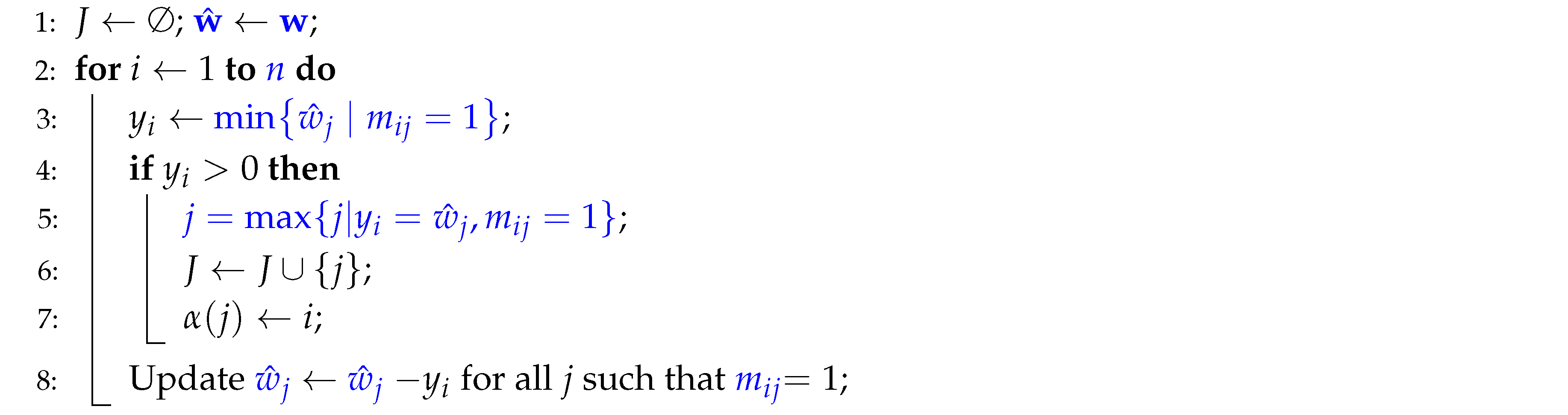
This connection enables us to modify and simplify Hoffman et al.’s original algorithms, Algorithms 1 and 2, to yield Algorithms 3 and 4. We present Algorithms 3 and 4 below with the necessary line-by-line transformations.
To modify and simplify Algorithm 1 into Algorithm 3, the following line-by-line adjustments (highlighted in blue) were made:
- Line 1: Replace with and with .
- Line 2: Adjust the loop range from m to n.
- Line 3: Simplify the min calculation from to .
- Lines 5 and 6: Replace the original lines with the simplified expression . Note that in the simplified algorithm, is unnecessary in Line 3. Therefore, if , then from must equal for some j. Thus, choosing the largest j such that can be expressed equivalently as .
- Line 9: Substitute each with and with in the update statement.
| Algorithm 3: Simplified Algorithm for |
 |
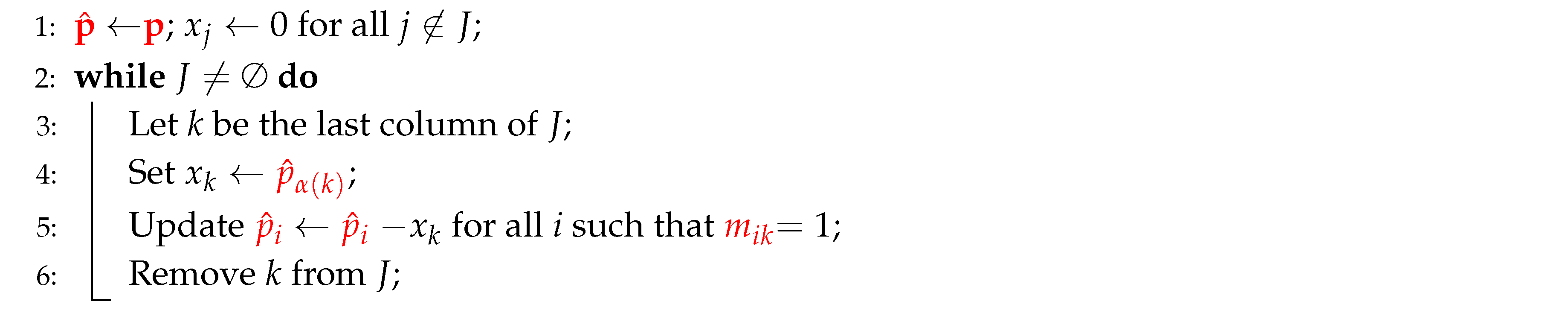
To modify and simplify Algorithm 2 into Algorithm 4, we made the following adjustments (highlighted in red):
- Line 1: Change to . Replace with .
- Line 4: Adjust to .
- Line 5: Replace with . Replace with .
- Remove Lines 7 and 8, since they are unnecessary in the simplified algorithm for .
| Algorithm 4: Simplified Algorithm for with Totally Balanced Matrices |
 |
By Theorem 4, the linear program and its dual are solvable in time for weighted strongly chordal graphs G with vertices in strong elimination ordering, and Algorithms 3 and 4 can provide integer optimal solutions for and . Thus, the -domination problem for weighted strongly chordal graphs can be solved in time. □
3.4. Optimized Algorithms with Enhanced Data Structures
In the previous section, we established that the linear program and its dual are special cases of the problems tackled by Hoffman et al.’s algorithms. This enables us to apply their method directly to solve these programs in time. Hoffman et al.’s algorithms are robustly constructed around the relationships between totally balanced matrices, greedy matrices, and linear programs, using the strengths of matrix structures and concepts from linear and integer programming. In contrast, the closed neighborhood matrices in are closely tied to graph adjacency structures.
The adjacency-list representation, as discussed in Section 2.1, plays a crucial role in enhancing the efficiency of Algorithms 3 and 4. By incorporating optimized data structures for critical steps in these algorithms, we improve the overall time complexity from to , where n represents the number of vertices, and m represents the number of edges in a graph. Since the maximum number of edges in a graph is , this improvement makes the algorithms particularly effective for sparse strongly chordal graphs when . Theorem 6 demonstrates how to obtain the desired time complexity.
Theorem 6.
For weighted strongly chordal graphs with n vertices arranged by strong elimination ordering, the -domination problem can be solved in time, where m is the number of edges in G.
Proof.
We begin with demonstrating how each line of Algorithm 3 relates to the adjacency list and other optimized data structures and the running time of each line based on the adjacency list representation and the number of vertices (n) and edges (m):
| Algorithm 3: Simplified Algorithm for |
 |
-
Line 1:This line initializes the set J to keep track of selected indices j and makes a copy of the vector as . This step does not directly involve the adjacency list, as it’s a basic initialization of variables. We implement J as an array with n entries and initialize the array with each entry set to zero. This array structure allows us to store specific information about each element efficiently, and each entry can be accessed, updated, or retrieved in time. The initialization step takes time.
-
Line 2:This loop iterates over each index i, where n corresponds to the number of constraints equal to the number of vertices. It executes n times in total. For each iteration, it processes Lines 3–8.
- Line 3: For each i, the algorithm assigns the minimum value among the entries for all j such that . Clearly, means . Using the adjacency list, the algorithm can directly access all neighbors of , including itself, in time.
-
Line 4:This line checks whether the calculated value is greater than 0. It can be done in time
-
Lines 5-7: This block finds the largest j for i such that and .The adjacency list helps here by providing access to each index j of , allowing the algorithm to identify all possible values of j where . Once the appropriate j is found, J and are updated. Since J is an array, the operation is translated to setting . Conversely, J does not contain some k if . We also implement the operation by an array. The operation is translated to setting .Hence, the steps take time.
-
Line 8:This line updates for each index j of vertices , subtracting from . Using the adjacency list, the algorithm can efficiently locate each j where and apply the update only to those specific j values for vertices .
The overall time complexity depends on the sum of all neighbor operations across vertices, yielding
where n is the number of vertices and m is the number of edges.
We next demonstrate how each line of Algorithm 4 relates to the adjacency list and other optimized data structures and the running time of each line based on the adjacency list representation and the number of vertices (n) and edges (m):
| Algorithm 4: Simplified Algorithm for with Totally Balanced Matrices |
 |
-
Line 1: This line initializes as a copy of and sets for all .To set for all , we implement a stack and set it to be empty. Then, we visit each entry for , set if , and push j into the stack if . After visiting all entries of J, we delete J and rename with J. All operations can be done in time. Since also has n entries, copying and takes time.
-
Line 2 (While Loop): The loop runs until J is empty, so the number of iterations depends on the number of elements in J. Clearly, it executes at most n times. Each iteration involves Lines 3–6, so we analyze each of these lines within the context of a single iteration.
- Line 3: Select the last column k from J. In other words, we have to select the largest index k of J with . Since we have implemented a stack, pushing each index j with into the stack from smallest one to the largest one, deleting J, and renaming the stack with J and deleting . Therefore, selecting the last column of J is equivalent to popping an element from J. Hence, it takes time.
- Line 4: Set based on . Retrieving the value from and assigning takes time.
- Line 5: Update for all i such that . Since , this operation iterates over each index i of vertices . Using the adjacency list, this step takes for each iteration.
- Line 6: Remove k from J. J is implemented as a stack. Removing the last element takes time.
The overall time complexity of the algorithm is:
where n is the number of vertices and m is the number of edges in the graph. This linear time complexity makes the algorithm efficient for sparse graphs.
Following the discussion above, Algorithms 3 and 4 both run in time. Consequently, the theorem holds. □
4. Total -Domination in Weighted Chordal Bipartite Graphs
The total -domination problem in weighted chordal bipartite graphs can be efficiently solved by structural properties of these graphs. Specifically, we demonstrate how the neighborhood matrix of a chordal bipartite graph ordered by its weak elimination ordering forms a greedy matrix in standard greedy form. The following lemma establishes the foundational connection between weak elimination orderings and greedy matrices.
Lemma 4.
If the vertices of a chordal bipartite graph are ordered by its weak elimination ordering, then the neighborhood matrix of the graph is a greedy matrix in standard greedy form.
Proof.
Let G be a chordal bipartite graph with the vertices ordered by its weak elimination ordering , and let be the neighborhood matrix of G. Since the neighborhood matrix of a chordal bipartite graph is totally balanced [49], is totally balanced. We now check if contains the -matrix as a submatrix:
Assume that contains the -matrix as a submatrix, shown below with entries chosen by rows and columns , where and :
Since is a neighborhood matrix, each is 0 for . It imples that , , and . Furthermore, as bipartite graphs contain only cycles with even number of vertices, if , then , and would form a cycle of odd number of vertices, which is impossible. Thus, .
Consider three cases:
- Case 1:. Then, , and are all vertices of . Since is adjacent to both and , the neighborhood relationship must hold. As , it follows that . However, this implies that is adjacent to , which contradicts the assumption that and are not adjacent.
- Case 2:. In this case, , and are all vertices of . Since is adjacent to both and , the neighborhood relationship must hold. Consequently, implies . However, this contradicts the assumption that and are not adjacent.
- Case 3:. Here, , and are again vertices of . By reasoning similar to Case 2, the adjacency of to both and implies . Since , we deduce that , which means and are adjacent. This contradicts the assumption that and are not adjacent.
These cases confirm that is totally balanced and excludes the -matrix as a submatrix. By Claim 1, we conclude that the neighborhood matrix of a chordal bipartite graph ordered by its weak elimination ordering is a greedy matrix in standard greedy form. □
The following lemma is similar to Lemma 1. It allows us to concentrate exclusively on non-negative vertex weights ().
Lemma 5.
Let w be a vertex-weight function of a graph , and let represent the the minimum labeling weight of a total -dominating function for . Define and let be a vertex-weight function such that for each . Then, .
Proof.
This lemma can be proved by the arguments similar to those for proving Lemma 1. □
Let G be a chordal bipartite graph with the vertices arranged in weak elimination ordering with as its neighborhood matrix. Let , , and , where for .
The total -domination problem for weighted chordal bipartite graphs can be formulated as the following integer linear program :
Let be the linear relaxation of , and let be the dual program of . We present the formulations of P, D, , and together below:
Theorem 7.
For weighted chordal bipartite graphs with n vertices arranged by its weak elimination ordering, the total -domination problem can be solved in time, where m is the number of edges in G.
Proof.
The proof proceeds in three steps:
- Neighborhood Matrix Properties: By Lemma 4, we have established that for a weighted chordal bipartite graph with n vertices arranged by its weak elimination ordering, the neighborhood matrix of G is a greedy matrix in standard greedy form. This property ensures that the constraints of the total -domination problem are well-structured for efficient computation.
- Connection to Linear Programs: The primal and dual linear programs, and , for the weighted chordal bipartite graphs are specific instances of the linear programs P and D, where and the vector is absent. These simplifications reduce the computational overhead associated with solving the general cases.
- Efficient Computation: Using arguments similar to those in the proofs of Theorems 5 and 6, we use the greedy matrix property of and advanced primal-dual algorithms to solve the relaxed problem efficiently. Optimized data structures ensure that each step in the algorithm operates in linear time relative to the size of the graph.
Combining these observations, the total -domination problem for weighted chordal bipartite graphs can be solved in time. □
5. Total -Tuple Domination and -Tuple Domination
The k-tuple domination and total k-tuple domination problems are fundamental in graph theory, with applications in optimization and network analysis. In this section, we investigate these problems for weighted proper interval graphs and weighted convex bipartite graphs. Utilizing structural properties of these graph classes, we formulate integer linear programs with totally unimodular constraint matrices, enabling efficient solutions via linear relaxations.
5.1. Integer Linear Programs with Totally Unimodular Matrices
Totally unimodular matrices allow integer solutions to be obtained directly from linear relaxations, making them crucial in solving the k-tuple and total k-tuple domination problems efficiently. This section presents our results about totally unimodular matrices and their applications.
5.1.1. Problem Formulations
Let be a weighed graph with n vertices and m edges. The k-tuple domination problem for is formulated as an integer linear program :
where is the closed neighborhood matrix of G, is the weight vector, and is a k-vector. Its linear relaxations is
To incorporate the constraint into the standard inequality framework, we express it equivalently as:
This transformation allows us to maintain a unified form for all constraints. Using this approach, the linear program can be rewritten as:
where , , is the identity matrix, and is a 1-vector.
Similarly, the total k-tuple domination problem is formulated as an integer linear program :
where is the neighborhood matrix. Its linear relaxation can be formulated as:
where , , is the identity matrix, and is a 1-vector.
5.1.2. Fundamental Lemmas on Totally Unimodular Matrices
In this section, we present our fundamental lemmas on totally unimodular matrices.
Lemma 6.
Let be a totally unimodular matrix, and let be the identity matrix. Then, the matrix
is also totally unimodular.
Proof.
It is clear that the matrix is totally unimodular, as each determinant of any square submatrix of evaluates to or 1, satisfying the definition of total unimodularity. Let be any square submatrix of .
First, if the rows of are formed exclusively from either or , then is totally unimodular because and satisfy the definition of total unimodularity by ensuring that every determinant of their square submatrices is in .
Next, consider the case where the rows of are formed from both and . We compute using the Laplace expansion along a row i formed from . By the definition of Laplace expansion:
where is the square submatrix obtained by removing the i-th row and j-th column from .
Since row i comes from , it has at most one nonzero entry, which is . This means that:
where s is a non-negative integer determined by the row and column indices of the nonzero entry.
If still contains rows from , we recursively apply the Laplace expansion and remove rows and columns associated with . Each step multiplies the determinant by , with . Eventually, the process reduces to a square submatrix of .
Since satisfies the definition of total unimodularity, every determinant of its square submatrices is in . Therefore, as well.
Thus, is totally unimodular. □
Lemma 7.
Let be a totally unimodular matrix, and let be the identity matrix. Then, the matrix
is also totally unimodular.
Proof.
By Lemma 6, we know that the matrix
is totally unimodular. Take the transpose of to obtain . The determinant of each square submatrix remains unchanged by transposing, so for each square submatrix of . Consequently, is a totally unimodular matrix. □
Theorem 8
([45]). Let be an integral matrix. Then, is totally unimodular if and only if for each integral vector , the polyhedron
is integral.
Lemma 8.
Let be an integral matrix. Then, is totally unimodular if and only if for each integral vector , the polyhedron
is integral.
Proof.
Assume that contains r rows. By the properties of determinants under scalar multiplication ([47]), for each square submatrix of , we have
If is totally unimodular, then , which implies that is totally unimodular. Let be an integer vector. Clearly,
By Theorem 8, the polyhedron is integral. Therefore, is also integral.
Conversely, if is integral, then so is . By Theorem 8, is totally unimodular. Following the same reasoning as above, is therefore also totally unimodular.
Thus, the lemma holds in both directions. □
Lemma 9.
Let be a totally unimodular matrix. For each integral vector , the polyhedron
is integral.
Proof.
It is clear that the polyhedron is equivalent to the following:
Following Theorem 8 and Lemma 8, the polyhedra and are integral. Therefore, is integral. □
5.2. k-Tuple Domination in Weighted Proper Interval Graphs
We have formulated the k-tuple domination problem for weighted graphs as the integer linear program . For weighted proper interval graphs, solving is equivalent to directly solving the k-tuple domination problem.
The following lemma establishes a critical connection between the closed neighborhood matrices of weighted proper interval graphs and totally unimodular matrices. This connection enables to be solved efficiently by addressing its linear relaxation .
Lemma 10.
The closed neighborhood matrix of a weighted proper interval graph is totally unimodular.
Proof.
The lemma follows from two established results:
□
Theorem 9.
The k-tuple domination problem for weighted proper interval graphs can be solved in the running time of
where n is the number of vertices, and δ is the desired accuracy within the range
Proof.
Following Lemmas 6, 8, and 10, we know that the closed neighborhood matrix of G and the constraint matrix in are totally unimodular, and the polyhedron of is integer. Therefore, the optimal objective values of and are equal. Thus, solving is equivalent to finding an integral solution to . This implies that the total k-tuple domination problem for weighted convex bipartite graphs can be solved by computing an integral solution to .
Recently, van den Brand [55] derandomized the algorithm Cohen et al. [56] to achieve that linear programs of the form with no redundant constraints can be solved in the running time
where n is the number of decision variables, is the exponent of matrix multiplication, is the dual exponent of matrix multiplication, and is the desired accuracy within the range . Williams et al. [57] established and . This yields a simplified complexity of .
The linear program is . To solve by van den Brand’s algorithm, we transform into the form using slack variables. The transformation steps are as follows:
-
Introduce Slack Variables.Convert the inequality into an equality by introducing slack variables. Rewrite it as:where is a vector of slack variables. This ensures each constraint in the original inequality has a corresponding non-negative slack variable.
-
Rewrite as Equalities.Rearrange the equality above as:Define a new vector , so we can express the constraints in matrix form as:
-
Extend the Objective Function.Since the original objective function is , extend it to include the slack variables by setting:where is a zero vector. This ensures that the slack variables do not affect the objective function.
Thus, the transformed linear program becomes:
where , , , and .
We verify the correctness and analyze the time complexity of this transformation by confirming that the feasible sets of and objective functions of the original and transformed problems are equivalent. The steps are as follows:
-
Converting Inequalities to Equalities via Slack VariablesIn , the inequality restricts so that each entry of is at least the corresponding entry of . To convert this inequality into an equality, we introduce a vector of slack variables , rewriting it as:This ensures that holds if and only if there exists a non-negative vector such that . Since has rows and n columns, the vector consists of entries. Setting up the slack variables takes time.
-
Reformulating Constraints with Augmented MatricesWe define and rewrite the equality as:where and . This matrix formulation ensures that each slack variable directly accounts for the surplus required to satisfy each inequality. Constructing requires combining with , and constructing requires combining with .The matrix has rows and columns. The vector has rows and one column, resulting in an augmented matrix, which takes time. Hence, the step can be done in time.
-
Ensuring Equivalence of Feasible Sets ofIn the original linear program, the feasible region is defined by all such that . In the transformed linear program, the feasible region is defined by all non-negative vectors that satisfy . Clearly,This establishes that the transformation preserves the feasible region.
-
Ensuring Equivalence of Objective FunctionsThe original objective function depends only on , so in the transformed program, we extend it by defining , where is a zero vector. This construction prevents the slack variables from influencing the objective function, so that the objective in the transformed program is identical to the original objective. Extending the objective vector takes time.
Having verified that the transformation preserves both the feasible region and the objective function, we conclude that the transformation is correct with the time complexity of .
Since is totally unimodular, Lemmas 7 and 9 imply that is totally unimodular, and the polyhedron of the transformed linear program is integer.
Despite the transformed linear program containing variables, it can still be solved in time. Consequently, the linear relaxation runs in time of:
□
5.3. Total k-Tuple Domination in Weighted Convex Bipartite Graphs
In this subsection, we explore the total k-tuple domination problem in weighted convex bipartite graphs. In Section 5.1.1, we formulated the total k-tuple domination problem for weighted graphs as the integer linear program . For weighted convex bipartite graphs , solving is equivalent to directly solving the total k-tuple domination problem.
To establish a connection between the neighborhood matrices of weighted convex bipartite graphs and totally unimodular matrices (as discussed in Section 5.1 and Section 5.2), we begin by examining the neighborhood matrix of a convex bipartite graph.
Figure 9 illustrates a convex bipartite graph , where and .
The neighborhood matrix of G is shown below:
The matrix is partitioned into four blocks: , , , and . Since G is bipartite, no two vertices in X or Y are adjacent. Therefore, and are zero-matrices. Moreover, the adjacency property ensures that every column of has consecutive ones. Then, has the consecutive ones property for columns. The block is the transpose of because of the symmetry of a neighborhood matrix of a graph.
Lemma 11.
Let be a square matrix partitioned as
where is a zero-matrix, and and are square matrices with . Then,
Proof.
By a factorization involving the Schur complement [58], we have
where and contribute independently to the determinant. Since , it follows that
Next, let
To transform into , we perform column exchanges. Each column exchange introduces a sign change in the determinant. Therefore, we have
where s is the number of column exchanges.
Since , and sign changes do not affect the magnitude of the determinant, we conclude
□
Theorem 10.
Let be a convex bipartite graph, where the ordering of X satisfies the adjacency property. Then, the neighborhood matrix of G is totally unimodular.
Proof.
Let and . The neighborhood matrix of G, an matrix, can be partitioned as
where Since G is bipartite, and are zero-matrices.
The adjacency property of G ensures that satisfies the consecutive ones property for columns. By Theorem 1, is totally unimodular. Since and the transpose of a totally unimodular matrix is also totally unimodular, is totally unimodular.
To verify that is totally unimodular, we show that every square submatrix of satisfies . Assume that is composed of p rows and p columns, where . We consider three cases based on the structure of .
Case 1: Is a Submatrix of a Single Block.
If is a submatrix of or , it is a zero-matrix, so . If is a submatrix of or , the total unimodularity of and ensures .
Case 2: Includes Rows and Columns from Exactly Two Blocks.
The rows and columns of are from two blocks, and , and , and , or and . Since and are zero-matrices, at least one row or column of is entirely zero, implying .
Case 3: Includes Rows and Columns from All Four Blocks.
We partition as
where
In this case, is a submatrix of for . Since and are submatrices of zero-matrices, they are zero-matrices themselves. This reduces to a dependency on and . We analyze based on the dimensions of the submatrices.
Case 3.1: .
In this case, . We partition as
where
Here, is a zero-matrix, and both and are square matrices. Notably, contains a column of zeros because . We have . Since is a submatrix of , it preserves totally unimodularity, and thus . By Lemma 11, .
Case 3.2: .
In this case, . We partition as
where
Here, is a zero-matrix, and both and are square matrices. Notably, contains a row of zeros because . We have . Since is a submatrix of , it preserves totally unimodularity, and thus . By Lemma 11, .
Case 3.3: .
In this case, . We partition as
where
Here, is a zero-matrix, and both and are square matrices. Since and are submatrices of totally unimodular matrices, their determinants satisfy and . By Lemma 11, .
In all subcases, . Therefore, the neighborhood matrix of the convex bipartite graph G is totally unimodular. □
Theorem 11.The total k-tuple domination problem for weighted convex bipartite graphs can be solved in the running time of
where n is the number of vertices in G, and δ is the desired accuracy within the range .
Proof. By Lemma 6, Lemma 8, and Theorem 10, the neighborhood matrix of G and the constraint matrix in are totally unimodular. Consequently, the polyhedron associated with is integer, meaning that the optimal objective values of and are equal.
Thus, solving is equivalent to finding an integral solution to . This implies that the total k-tuple domination problem for weighted convex bipartite graphs can be solved by computing an integral solution to .
Following arguments analogous to those used in the proof of Theorem 9, we conclude that the total k-tuple domination problem can be solved in the running time of
□
Conclusions and Future Directions
This paper investigates the complexity and algorithmic solutions for -domination, k-tuple domination, and their total domination variants in weighted subclasses of chordal graphs and bipartite graphs. The primary contributions of this work are as follows:
- Developing efficient time algorithms for -domination in weighted strongly chordal graphs and total -domination in weighted chordal bipartite graphs.
- Establishing the running time of for k-tuple and total k-tuple domination in weighted proper interval graphs and convex bipartite graphs. This result improves the running time for the k-tuple domination problem in unit proper interval graphs.
- Extending theoretical models to vertex-weighted graph settings, bridging gaps in the existing research on weighted graph domination.
- Leveraging linear and integer programming techniques, supported by totally balanced and totally unimodular matrices, to provide formal proofs of correctness and efficiency for the proposed algorithms.
These results advance both the theoretical understanding and computational efficiency of domination problems in weighted graph classes.
Future work can extend these domination techniques to other weighted graph classes, including real-world network applications and dynamic graph settings. Additionally, integrating these approaches with advanced optimization techniques, such as parallel computation and distributed systems, may yield even more efficient and scalable algorithms.
Funding
This research received no external funding.
Data Availability Statement
Data is contained within the article or supplementary material.
Acknowledgments
The author sincerely thanks the reviewers for their insightful comments and suggestions, which have greatly improved this paper’s clarity, analysis, and overall quality. Their constructive feedback and dedication to advancing research in this field are deeply appreciated.
Conflicts of Interest
The author declares no conflicts of interest.
References
- Hedetniemi, S.T.; Laskar, R.C. (Eds.), Special Volume: Topics on Domination, Discrete Mathematics, Vol. 86, No.1-3, December 1990.
- Haynes, T.W.; Hedetniemi, S.T.; Slater, P.J. (Eds.), Fundamentals of Domination in Graphs, Marcel Dekker, New York, 1998.
- Haynes, T.W.; Hedetniemi, S.T.; Slater, P.J. (Eds.), Domination in Graphs: Advanced Topics, Marcel Dekker, New York, 1998.
- Haynes, T.W.; Hedetniemi, S.T.; Henning, M.A. (Eds.), Topics in Domination in Graphs,Developments in Mathematics, Vol. 64, Springer, Cham, 2020.
- Haynes, T.W.; Hedetniemi, S.T.; Henning, M.A. (Eds.), Structures of Domination in Graphs, Developments in Mathematics, Vol. 66, Springer, Cham, 2021.
- Haynes, T.W.; Hedetniemi, S.T.; Henning, M.A. (Eds.), Domination in Graphs: Core Concepts, Springer Monographs in Mathematics, Springer, Cham, 2023.
- Henning, M.A.; Yeo, A. Total Domination in graphs, Springer Monographs in Mathematics, Springer, 2013.
- Argiroffo, G.; Leoni, V.; Torres, P. On the complexity of {k}-domination and k-tuple domination in graphs. Inform. Process. Lett. 2015, 115, 556–561. [Google Scholar] [CrossRef]
- Pradhan, D. Complexity of certain functional variants of total domination in chordal bipartite graphs. Discrete Math. Algorithms Appl. 2012, 4, Article 1240045. [Google Scholar] [CrossRef]
- Argiroffo, G.; Leoni, V.; Torres, P. Complexity of k-tuple total and total {k}-dominations for some subclasses of bipartite graphs. Inform. Process. Lett. 2018, 138, 75–80. [Google Scholar] [CrossRef]
- He, J.; Liang, H. Complexity of total {k}-domination and related problem. In Proceedings of the FAW-AAIM 2011, LNCS 6681; pp. 147–155.
- Liao, C.; Chang, G.J. k-tuple domination in graphs. Inform. Process. Lett. 2003, 87, 45–50. [Google Scholar] [CrossRef]
- Li, P.; Wang, A.; Shang, J. A simple optimal algorithm for k-tuple dominating problem in interval graphs. J. Comb. Optim. 2023, 45, Article Number 14. [Google Scholar] [CrossRef]
- Dobson, M.P.; Leoni, V.; Lopez Pujato, M.I. Efficient algorithms for tuple domination on co-biconvex graphs and web graphs. arXiv preprint 2022, arXiv:2008.05345. [Google Scholar]
- Lee, C.-M.; Chang, M.S. Variations of Y-dominating functions on graphs. Discrete Math. 2008, 308, 4185–4204. [Google Scholar] [CrossRef]
- Chiarelli, N.; Hartinger, T.R.; Leoni, V.A.; Lopez Pujato, M.I.; Milaniĉ, M. New algorithms for weighted k-domination and total k-domination problem in proper interval graphs. Theor. Comput. Sci. 2019, 795, 128–141. [Google Scholar] [CrossRef]
- Li, P.; Li, X.; Liu, J.-B.; Shang, J. Optimized algorithms for problems related to weighted k-domination, k-tuple domination, and total k-domination for unit interval graphs, 2024. Available at SSRN: https://ssrn.com/abstract=4725957 or http://dx.doi.org/10.2139/ssrn.4725957.
- Brandstädt, A.; Le, V. B.; Spinrad, J. P. Graph Classes: A Survey. Society for Industrial and Applied Mathematics, 1999.
- Hoffman, A.J.; Kolen, A.W.J.; Sakarovitch, M. Totally-balanced and greedy matrices. Siam J. Alg. Disc. Meth. 1985, 6, 721–730. [Google Scholar] [CrossRef]
- Argiroffo, G.; Leoni, V.; Torres, P. On the complexity of the labeled domination problem in graphs. Int. Trans. Oper. Res. 2017, 24, 355–367. [Google Scholar] [CrossRef]
- Bonomo-Braberman, F.; Gonzalez, C.L. A new approach on locally checkable problems. Discrete Appl. Math. 2022, 314, 53–80. [Google Scholar] [CrossRef]
- Tan, H.; Liu, L.; Liang, H. Total {k}-domination in special graphs. Math. Found. Comput. 2018, 1, 255–263. [Google Scholar] [CrossRef]
- Lee, C.-M. R-total domination on convex bipartite graphs. J. Comb. Math. Comb. Comput. 2012, 81, 209–224. [Google Scholar]
- Lee, C.-M. The complexity of total k-domatic partition and total R-domination on graphs with weak elimination orderings. Int. J. Comput. Math.: Comput. Syst. Theory, 2020, 5, 134–147. [Google Scholar] [CrossRef]
- Bonomo, F.; Brešar, B.; Grippo, L.N.; Milanič, M.; Safe, M.D. Domination parameters with number 2: interrelations and algorithmic consequences. Discrete Appl. Math. 2018, 235, 23–50. [Google Scholar] [CrossRef]
- Brešar, B.; Dorbec, P.; Goddard, W.; Hartnell, B.; Henning, M.A.; Klavžar, S.; Rall, D.F. Vizing’s conjecture: A survey and recent results. J. Graph Theory, 2012, 69, 46–76. [Google Scholar] [CrossRef]
- Cabrera-Martínez, A.; Conchado Peiró, A. On the {2}-domination number of graphs. AIMS Math. 2022, 7, 10731–10743. [Google Scholar] [CrossRef]
- Cabrera-Martínez, A.; Montejano, L.P.; Rodríguez-Velázquez, J.A. From w-domination in graphs to domination parameters in lexicographic product graphs. Bull. Malays. Math. Sci. Soc. 2023, 46, 109. [Google Scholar] [CrossRef]
- Cheng, Y.J.; Fu, H.L.; Liu, C.A. The integer {k}-domination number of circulant graphs. Discrete Math. Algorithms Appl. 2020, 12, Article 2050055. [Google Scholar] [CrossRef]
- Choudhary, K.; Margulies, S.; Hicks, I.V. Integer domination of Cartesian product graphs. Discrete Math. 2015, 338, 1239–1242. [Google Scholar] [CrossRef]
- Krop, E.; Davila, R.R. On a Vizing-type Integer Domination Conjecture. Theory Appl. Graphs, 2020, 7, Article 4. [Google Scholar] [CrossRef]
- Villamar, I.R.; Cabrera-Martínez, A.; Sánchez, J.L.; Sigarreta, J.M. Relating the total {2}-domination number with the total domination number of graphs. Discrete Appl. Math. 2023, 333, 90–95. [Google Scholar] [CrossRef]
- Zverovich, V. On general frameworks and threshold functions for multiple domination. Discrete Math. 2015, 338, 2095–2104. [Google Scholar] [CrossRef]
- Liao, C.; Chang, G.J. Algorthmic aspects of k-tuple domination in graphs. Taiwan. J. Math. 2002, 6, 415–420. [Google Scholar] [CrossRef]
- Dobson, M.P.; Leoni, V.; Nasini, G. The multiple domination and limited packing problems in graphs. Inform. Process. Lett. 2011, 111, 1108–1113. [Google Scholar] [CrossRef]
- Dobson, M.P.; Leoni, V.; Lopez Pujato, M.I. k-tuple and k-tuple dominations on web graphs. Mat. Contemp. 2020, 48, 31–41. [Google Scholar] [CrossRef]
- Bellmonte, R.; Vatshelle, M. Graph classes with structured neighborhoods and algorithmic applications. Theor. Comput. Sci. 2013, 511, 54–65. [Google Scholar] [CrossRef]
- Bui-Xuan, B.; Telle, J.A.; Vatshelle, M. Fast dynamic programming for locally checkable vertex subset and vertex partitioning problems. Theor. Comput. Sci., 2013, 511, 66–76. [Google Scholar] [CrossRef]
- Barman, S.C.; Mondal, S.; Pal, M. Minimum 2-tuple domianting set of permutation graphs. J. Appl. Math. Comput. 2013, 43, 133–150. [Google Scholar] [CrossRef]
- Sinha, A.K.; Rana, A.; Pal, A. The 2-tuple domination problem on trapezoid graphs. Ann. Pure Appl. Math. 2014, 7, 71–76. [Google Scholar]
- Sinha, A.K.; Rana, A.; Pal, A. , The 2-tuple domination problem on circular-arc graphs. J. Math. Inform. 2017, 8, 45–55. [Google Scholar] [CrossRef]
- Lan, J.K.; Chang, G.J. On the algorithmic complexity of k-tuple total domination. Discrete Appl. Math. 2014, 174, 81–91. [Google Scholar] [CrossRef]
- Lee, C.-M. Signed and minus total domination on subclasses of bipartite graphs. Ars Combinatoria 2011, 100, 129–149. [Google Scholar]
- Cormen, T.H.; Leiserson, C.E.; Rivest, R. L.; Stein, C. Introduction to Algorithms (4th ed.). MIT Press, 2022.
- Schrijver, A. Theory of linear and integer programming. John Wiley & Sons, 1998.
- Diestel, R. Graph Theory (6th ed.). Springer Berlin, Heidelbergs, 2024.
- Strang, G. Introduction to linear algebra. Wellesley-Cambridge Press, 2022.
- Rose, D.J. Triangulated graphs and the elimination process. J. Math. Anal. Appl. 1970, 32, 597–600. [Google Scholar] [CrossRef]
- Farber, M. Characterizations of strongly chordal graphs. Discrete Math. 1983, 43, 173–189. [Google Scholar] [CrossRef]
- Uehara, R. Linear time algorithms on chordal bipartite and strongly chordal graphs. In Automata, Languages and Programming: 29th International Colloquium, ICALP 2002 Málaga, Spain, July 8–13, 2002, pp. 993-1004.
- Tardella, F. The fundamental theorem of linear programming: extensions and applications. Optimization 2011, 60, 283–301. [Google Scholar] [CrossRef]
- Khachiyan, L.G. A polynomial algorithm for linear programming. Doklady Akademii Nauk SSSR, 1979, 244, 1093–1096. [Google Scholar] [CrossRef]
- Karp, R.M. Reductibility among combinatorial problems. Complexity of computer computations, 1972, 1, 85–103. [Google Scholar]
- Scheinerman, E.R.; Ullman, D.H. Fractional Graph Theory: A Rational Approach to the Theory of Graphs. Dover Publications, INC. Mineola, New York, 2011.
- Van den Brand, J. A deterministic linear program solver in current matrix multiplication time. In Proceedings of the Fourteenth Annual ACM-SIAM Symposium on Discrete Algorithms, Society for Industrial and Applied Mathematics, 2020, 259-278.
- Cohen, M.B.; Lee, Y.T.; Song, Z. Solving linear programs in the current matrix multiplication time. J. ACM 2021, 68, 1–39. [Google Scholar] [CrossRef]
- Williams, V.V.; Xu, Y.; Xu, Z.; Zhou, R. New bounds for matrix multiplication: from alpha to omega. In Proceedings of the 2024 Annual ACM-SIAM Symposium on Discrete Algorithms (SODA), Society for Industrial and Applied Mathematics, 2024, pp. 3792-3835.
- Zhang, F. (Ed.) The Schur complement and its applications (Vol. 4). Springer Science & Business Media, 2006.
Figure 1.
A representation of a graph G. (a) The graph G with 4 vertices and 4 edges. (b) The adjacency-list representation of G.
Figure 1.
A representation of a graph G. (a) The graph G with 4 vertices and 4 edges. (b) The adjacency-list representation of G.
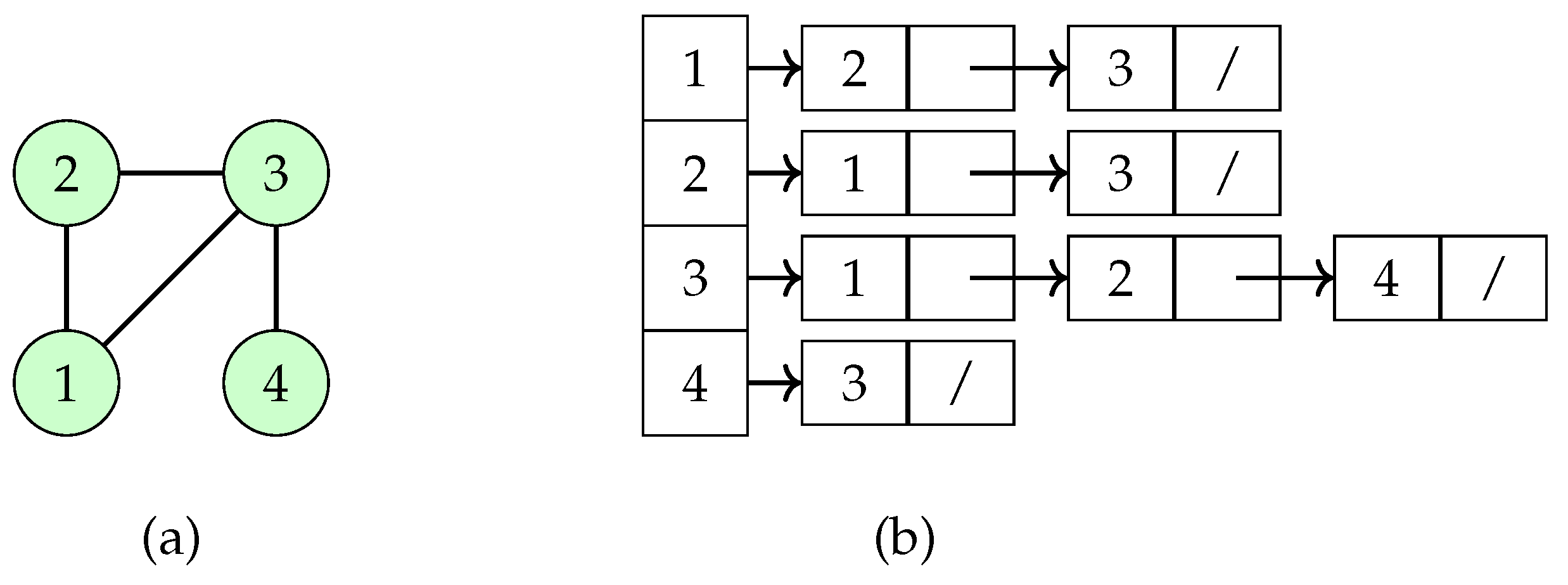
Figure 2.
Two sets and . (a) is a dominating set. (b) is a total dominating set.
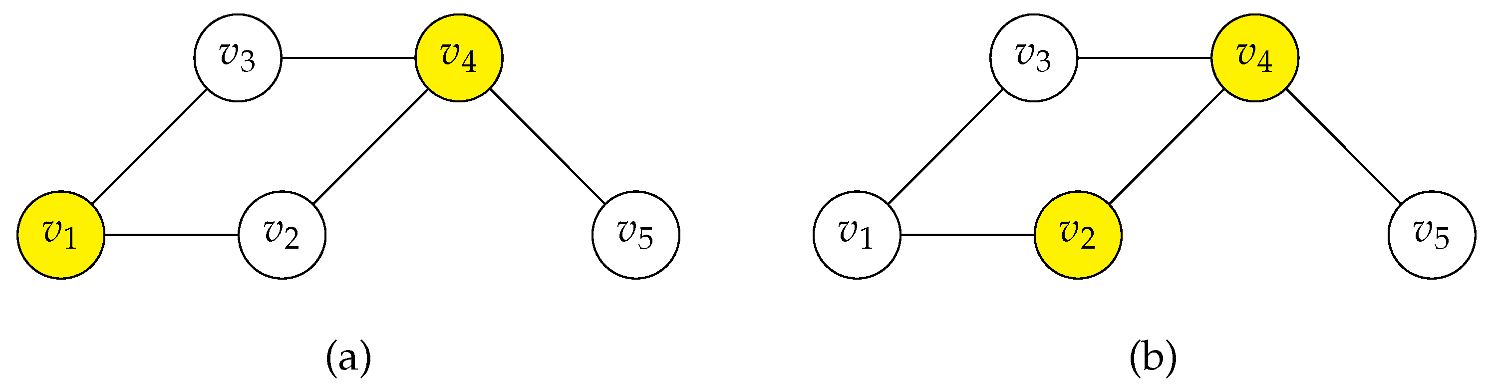
Figure 3.
A graph with six vertices.
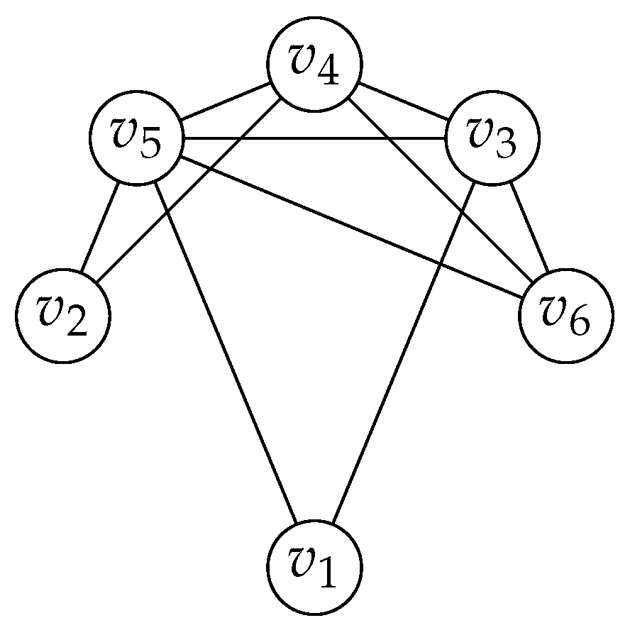
Figure 4.
Two chordal graphs. (a) A strongly chordal graph. (b) The Hajós graph (right).
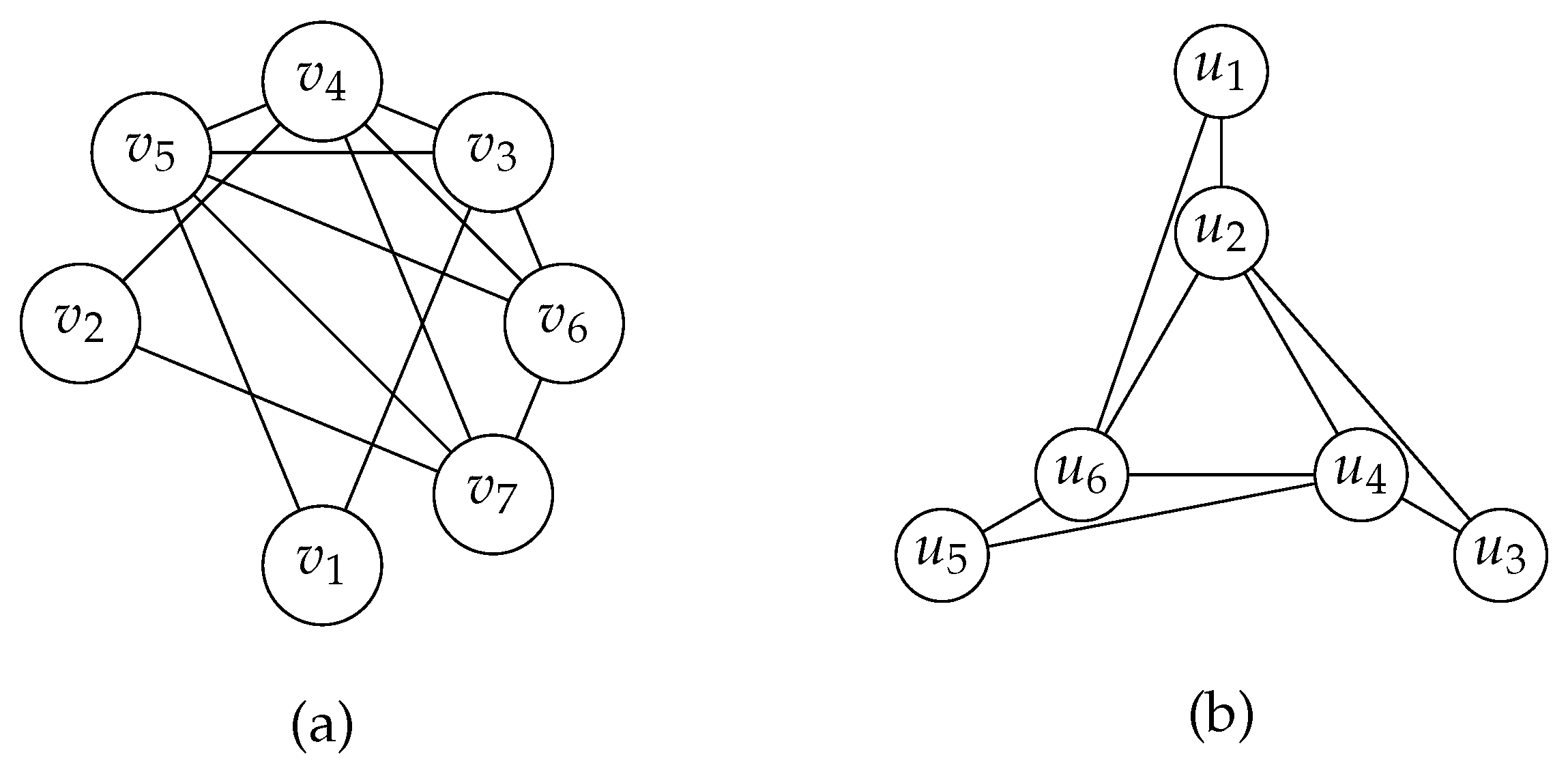
Figure 5.
Two graphs. (a) A bipartite graph with six vertices. (b) A graph with a cycle of three vertices.
Figure 5.
Two graphs. (a) A bipartite graph with six vertices. (b) A graph with a cycle of three vertices.
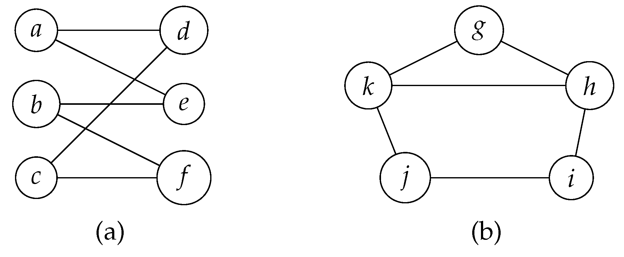
Figure 6.
Two bipartite graphs. (a) A chordal bipartite graph. (b) A bipartite graph with an induced cycle .
Figure 6.
Two bipartite graphs. (a) A chordal bipartite graph. (b) A bipartite graph with an induced cycle .
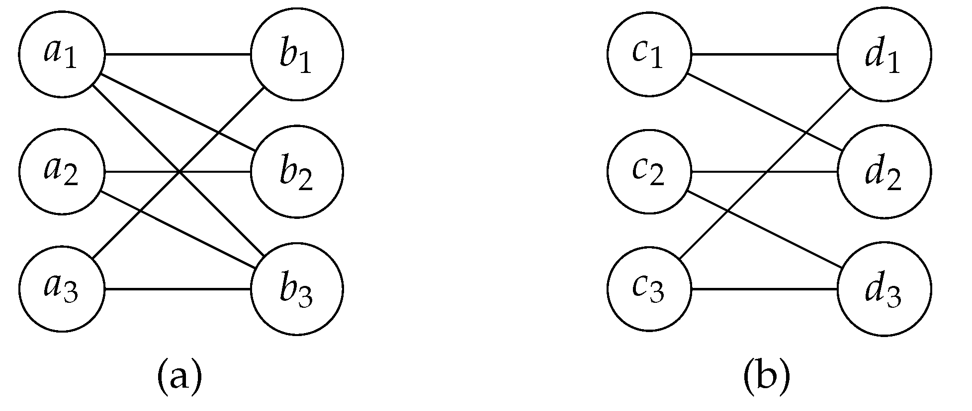
Figure 7.
An interval graph constructed from the intervals . The upper part shows the interval representation, and the lower part shows the corresponding graph.
Figure 7.
An interval graph constructed from the intervals . The upper part shows the interval representation, and the lower part shows the corresponding graph.
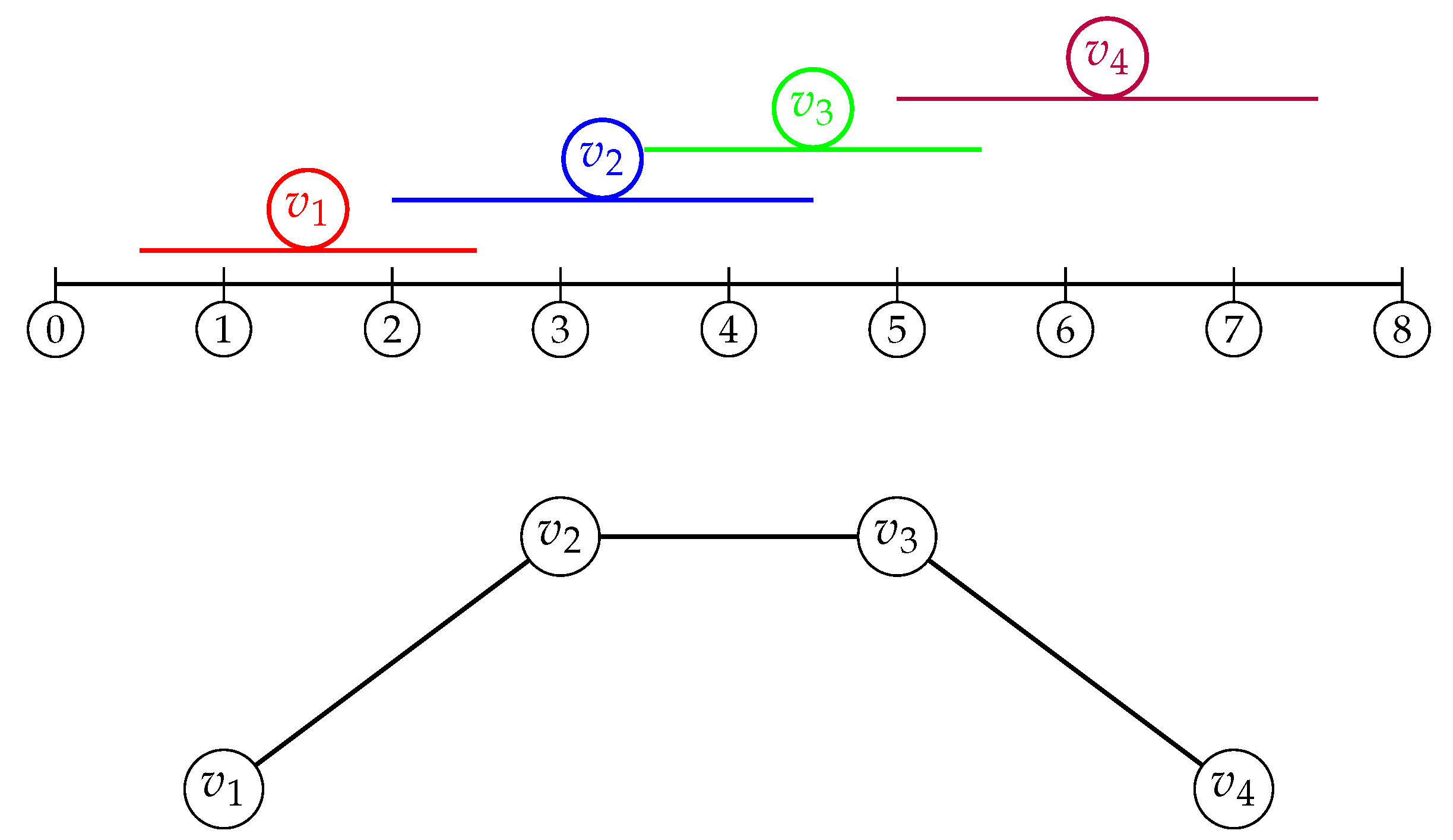
Figure 8.
A convex bipartite graph.
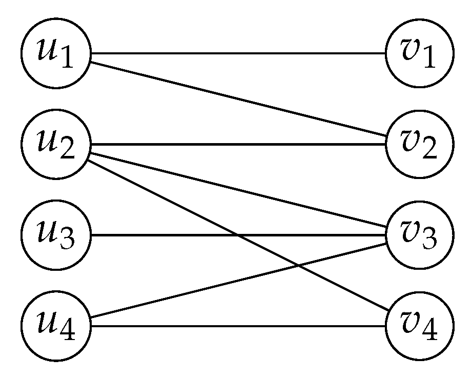
Figure 9.
A convex bipartite graph , where and . The graph satisfies the adjacency property for the ordering of X.
Figure 9.
A convex bipartite graph , where and . The graph satisfies the adjacency property for the ordering of X.
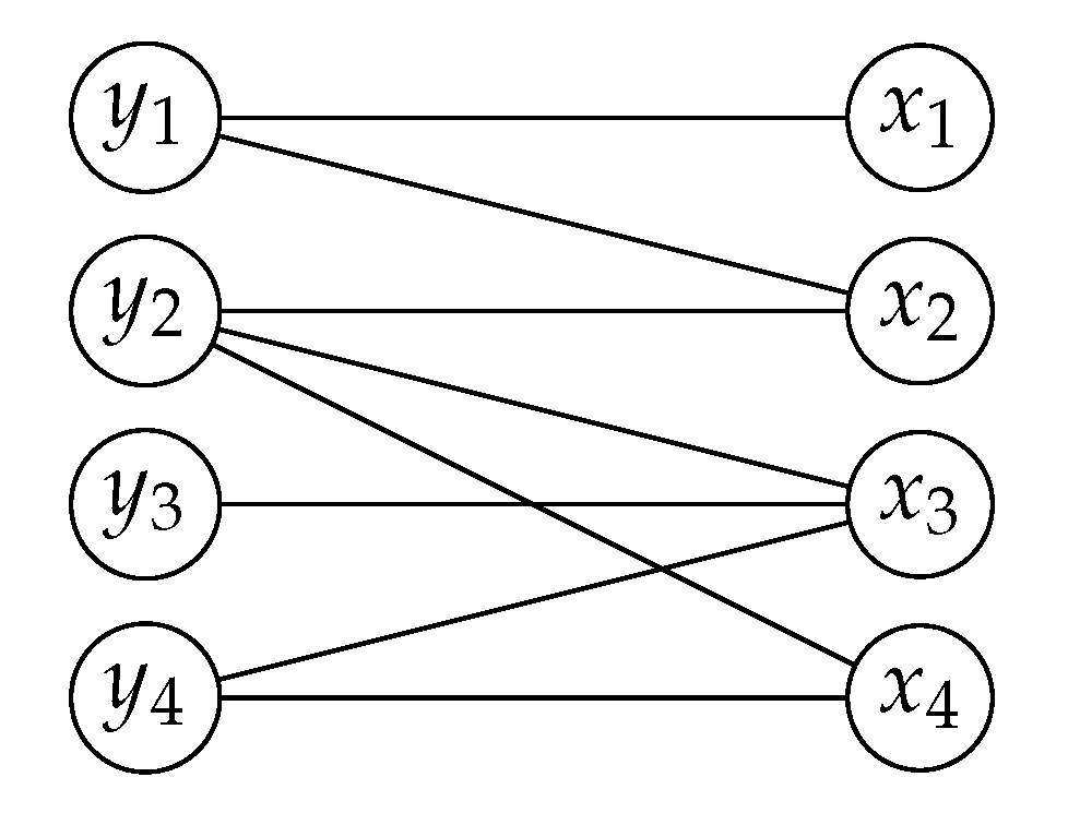

Table 1.
Values of dominating functions f and g, and membership in sets and for the graph in Figure 2.
Table 1.
Values of dominating functions f and g, and membership in sets and for the graph in Figure 2.
| Vertex v | In ? | In ? | ||
|---|---|---|---|---|
| 1 | 0 | Yes | No | |
| 0 | 1 | No | Yes | |
| 0 | 0 | No | No | |
| 1 | 1 | Yes | Yes | |
| 0 | 0 | No | No |
| Vertex v | |||
|---|---|---|---|
| 0 | |||
| 1 | |||
| 1 | |||
| 2 | |||
| 0 |
Table 3.
Labeling weights of the -dominating function f for the unweighted and weighted graphs.
| Vertex v | Weight | ||
|---|---|---|---|
| 2 | 0 | 0 | |
| 3 | 1 | 3 | |
| 1 | 1 | 1 | |
| 4 | 2 | 8 | |
| 2 | 0 | 0 | |
| Labeling Weight | 4 | 12 |
Table 4.
Labeling weights for a 2-tuple dominating function f and a total -tuple dominating function g in weighted and unweighted graphs.
Table 4.
Labeling weights for a 2-tuple dominating function f and a total -tuple dominating function g in weighted and unweighted graphs.
| Vertex v | Weight | ||||
|---|---|---|---|---|---|
| 2 | 1 | 0 | 2 | 0 | |
| 3 | 0 | 0 | 0 | 0 | |
| 1 | 0 | 1 | 0 | 1 | |
| 4 | 1 | 1 | 4 | 4 | |
| 2 | 1 | 1 | 2 | 2 | |
| 2 | 0 | 0 | 0 | 0 | |
| Labeling Weight | 3 | 3 | 8 | 7 |
Disclaimer/Publisher’s Note: The statements, opinions and data contained in all publications are solely those of the individual author(s) and contributor(s) and not of MDPI and/or the editor(s). MDPI and/or the editor(s) disclaim responsibility for any injury to people or property resulting from any ideas, methods, instructions or products referred to in the content. |
© 2024 by the author. Licensee MDPI, Basel, Switzerland. This article is an open access article distributed under the terms and conditions of the Creative Commons Attribution (CC BY) license (https://creativecommons.org/licenses/by/4.0/).
Copyright: This open access article is published under a Creative Commons CC BY 4.0 license, which permit the free download, distribution, and reuse, provided that the author and preprint are cited in any reuse.


