
Submitted:
22 May 2025
Posted:
23 May 2025
You are already at the latest version
Abstract
Researchers show a lot of interest in the probe of graph invariants with respect to graph products as it poses challenging questions and provides interesting insights. The graph invariants considered here are domination, total domination and captive domination numbers. Let G = (V, E) be a simple undirected graph. A set D⊆V(G) is called a dominating set if any v ∈ V(G) – D is adjacent to at least one element in D and the size of a minimum dominating set of G is called the domination number of G denoted by γ(G).D is called a total dominating set if any v ∈V(G) is adjacent to at least one element in D and the size of a minimum total dominating set of G is called the total domination number of G denoted by γt(G).The graph product taken up for investigation is the strong product of two path graphs. A motivation for this stems from the conjecture: Let Γ = CNN [n, m] be the (n, m)- dimensional CNN such that m, n ≥ 2. Then γΓ = n3m3raised in [1]. Here the CNN denotes cellular neural networks. In the language of graph theory, the Γ is isomorphic to the strong product of two path graphs denoted byPn⊠ Pm. In this paper, while disproving this conjecture for certain cases we also found the exact values of γΓ for all n and m by carefully analyzing the underlying structures for connection pattern. While doing so, we also end up with the exact values of γtPn⊠Pm and a few other results.
Keywords:
Domination number
; Total Domination Number
; Captive Domination Number
; Strong Product
MSC: 05C69
1. Introduction
Researchers are very much inclined to investigate graph invariants with respect to graph products, in particular on the Cartesian product, the lexicographic product, the direct product or tensor product and the strong product [2]. A primary reason is the fact that a lot of challenging questions, concerning products of graphs, provide interesting insights and new growths in probes of these graph invariants such as the domination number and its modifications. It all came into lime light with Vizing’s conjecture on the domination number of the Cartesian product of graphs, raised in [3], and led to the birth of various related concepts and techniques [4]. The domination number of the Cartesian product of paths was fully found only in 2011 [5], after several endavors resulted in distinct methods to graph domination problems.
An n × m grid graph G has the vertex set V = {: 1 ≤ i ≤ n, 1 ≤ j ≤ m} with two vertices and being adjacent if = and and are adjacent or if = and and are adjacent. The n × m grid graph can also be thought as a Cartesian product of two path graphs Pn and Pm, denoted by Pn × Pm of respective lengths n − 1 and m– 1.
The strong product of two graphs G and H denoted by G ⊠H has the vertex set V(G ⊠H) = V(G) × V(H). We say that a vertex () ∈ V(G × H) is adjacent to a vertex ∈ V(G × H) if and only if either = and () ∈ E(H) or () ∈ E(G) and = or ∈ E(G) and ()∈ E(H). Rarely some authors also refer to a strong product of two graphs as strong direct product or a symmetric composition [6].
A set D⊆V(G) is called a dominating set if any v ∈ V(G) – D is adjacent to at least one element in D and the size of a minimum dominating set of G is called the domination number of G denoted by γ(G).D is called a total dominating set if any v∈V(G) is adjacent to at least one element in D and the size of a minimum total dominating set of G is called the total domination number of G denoted by (G).D is called a captive dominating set, if it is a total dominating set and each element in D is adjacent to at least one element in V – D and the size of a minimal captive dominating set is called the captive domination number of G denoted by(G).
The γ of grid graphs has been probed for the past fifty years. A lot attempts have been made to get lower and upper bounds on . For detailed investigations of general bounds on , one can see [7,8,9,10,11]. Also probes have been made on specific bounds for small values of either n or m or both. The authors in [12] showed for 1 ≤ n ≤ 4 and all m. It was then carried to the cases of n = 5, 6 and all m by the authors in [13]. In [14] the authors adopted a computational method to find for n = 7, 8, m ≤ 500; n = 9, m ≤ 233; and n = 10, m ≤ 125. Some of the previous findings were subsequently verified to be true in [15]. Fisher in 1990’s introduced a new technique for finding γ for grid graphs. His work was not published but is explained in [16], where the values of for n≤ 19 and all m are listed. By appealing to a dynamic programming algorithm, the values of for n, m ≤ 29 were obtained in [17]. The authors in [17] also depicted the minimum dominating sets for square grid graphs up to a size of 29 × 29. The domination number concept finds a lot of applications in protection mechanisms and business networking [18]. For more one can refer to [19,20] and the references therein.
There are a variety of alterations on domination concept in graph. Some of them are total domination number, captive domination number, locating dominating number [21,22,23,24], independent dominating number [25,26], Roman dominating number [27,28] etc, The authors in [29] used the link among the existence of tiling’s in Manhattan metric with {1}-bowls and of Cartesian products of paths and cycles to derive the asymptotical values of the of these graphs and they further derived of certain cartesian products of cycles. Also, they studied the problem of for certain Cartesian products of two paths.
In this paper, motivated by the above works, we probe domination number, total domination number and captive domination number of strong product of graphs. In particular, the strong product of Pn and Pm .Another motivation for considering the strong product of graphs also stems from the work of the authors in [30] wherein they studied the relationship among the total k-domination number of the strong product of two graphs with the domination, k-domination and total k-domination numbers of the factors in the product. The idea of the exact value of the domination number can also applied to the multistep power consumption forecasting problem through smart grid electricity management. [31].
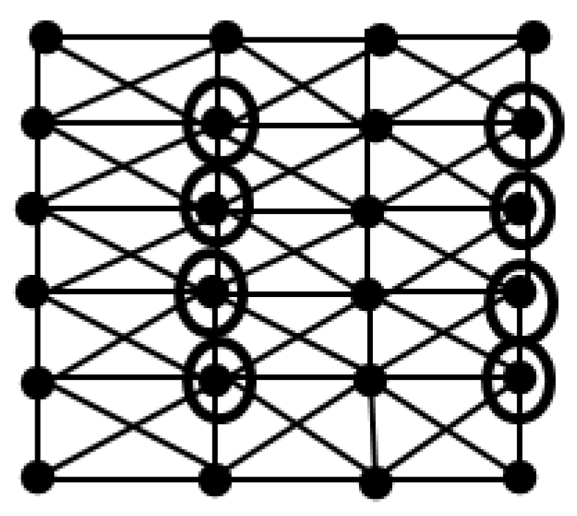
First we identify specific patterns lying in the graph Pn⊠Pm for various values of n and m and call them as Configurations. The minimum number of vertices required to dominate or totally dominate the rest of the vertices in such configurations are marked with a circle around them and are used in the proof of our results.
2. Domination number of strong product of path graphs
Theorem 2.1:
γ (Pn⊠Pm ) = r2if (n, m) = (3r, 3r-1) or (3r, 3r) or (3r-1, 3r) ;
r2 + r if (n, m) = (3r, 3r+1) or (3r-1, 3r+1) or (3r+1, 3r) or (3r+1, 3r-1).
Proof: We split the proof into various cases.
Case1: (n, m) = (3r, 3r)
We call a 3 × 3 mesh for r = 1 in a Type-A configuration. It is shown in Figure 1.
Note that each is an ordered pair of vertices for some 1≤ i, j ≤ 3r. It is easy to observe that D = {} is a minimum dominating set for the Type–A configuration. Here we also observe that a 3 × 3 mesh can be thought as an induced subgraph of. There are r2 Type A configurations in. Each such Type-A configuration yields one dominating element of that 3 × 3 mesh. Hence it is easy to see that a minimum dominating set of contains r2 elements. So γ() = r2.
Case 2: (n, m) =(3r, 3r-1).
For r =1, (n, m) =(3, 2), we see thatis a Type B configuration and it is shown in Figure 1.
So γ() = 1 = 12 = r2. For r =2, (n, m) =(6, 5). The graph is shows Figure 2
consists of two disjoint Type-A configurations one below the other and also on the left-hand side two disjoint Type B configurations one below the other. The minimum dominating set D for can be formed by adding the four elements indicated in Figure 2. So γ() = 4 = 22= r2. In general, there are r(r-1) disjoint Type-A configurations one below the other and one after the other to the left. Also there are r disjoint Type-B configurations one below the other to the left most Type A configurations. The minimum dominating set D of can be formed by adding all r(r-1) +r the marked elements. These marked elements in are chosen by following the pattern of selection indicated in Figure 2. So |D| = r2 -r + r = r2 and γ() = r2.
Case 3: (n, m) = (3r-1, 3r+1).
For r = 1, (n, m) = (2,4). The graph is shown in Figure 3.
Clearly it consists of a one Type B configuration and one 2 × 2 mesh fused with it. So γ() = 1+1 = 2 = 12 + 1 = r2 + r. For r =2, (n, m) = (5, 7). The graph is shown Figure 4.
It consists of 22fused Type A configuration and 2 fused Type B configurations. So the minimum dominating set D for can be formed by including all the marked elements shown in Figure 5. Therefore |D| = 22 + 2 = r2 + r = 6 andγ() = 22 + 2= 4 + 2 = 6 = r2 +r. In general, consists of r2fused Type A configurations and r fused type B configurations. So if D is the minimum dominating set then it will include all the marked elements of the respective configurations chosen by following the same pattern as indicated in Figure 1. So |D| = r2 + r and γ() = r 2+r.
The other cases can be handled in a similar manner.
3. Total Domination Number of Strong Product of Path Graphs
Theorem 3.1:
=2r2if (n, m) = (4r, 3r) or (4r, 3r-1);
= 2r2+r if (n, m) = (4r+1, 3r) or (4r+1, 3r-1);
= 2r2 +2r if (n, m) = (4r, 3r+1) or (4r+2, 3r) or (4r+2, 3r-1) or (4r+3, 3r) or
(4r+3, 3r-1);
= 2r2+3r+1 if (n, m) = (4r+1, 3r+1);
=2(r+1)2 if (n, m) = (4r+2, 3r+1) or (4r+3, 3r+1).
Proof: We split the proof into various cases.
Case 1: (n, m) = (4r,3r).
We call a 4 ×3 mesh in a Type C- Configuration and it is shown in Figure 1. Note that each is an ordered pair of vertices () for some 1 ≤ i ≤ 4r, 1 ≤ j ≤ 3r.
It is easy to observe that D = {} is a minimum total dominating set for Type C configuration. Here we also observe that a Type C configuration can be thought of as an induced subgraph of . There are r2 Type C configuration in. Each Type C configuration yields two dominating elements of that 4×3 mesh. Hence it is each to see that a minimum total dominating set of contains 2r2elements. So = 2r2.
Case 2: (n,m) = (4r+1,3r).
For r =1, (n,m) = (5, 3). Clearly = 2 ×12 +1= 2r2+r as D = {}totally dominates all other ’s for i = 1,2,3,4, 6,7,9,10,12,13,15.For r =2, (n,m) = (9,6). Clearly consists of two Type C configurations arranged side by side and two Type E configurations also arranged side by side but each one below their respective Type C configurations. So a minimum total dominating set D of will consists of 2 ×2 + 2 ×3 = 4 + 6 = 10 elements and hence = 10= 2 ×22+2. In general, there are (r-1)r Type C configurations arranged horizontally side by side and one after the other vertically and r Type E configurations arranged horizontally side by side below their respective Type C configurations. So a minimum total dominating set D of will consist of 2(r-1)r+ 3r= 2r2+r elements. So = 2r2+r.
Case 3: (n,m) = (4r+1, 3r-1).
For r = 1, (n,m) = (5,2) is called a Type F configuration and it is shown in Figure 1. Clearly D = {} is a minimum total dominating set. So = 3.
For r =2, (n,m) = (9,5). The graph is shown in Figure 5. It consists of one Type C, one Type D, one Type E and one Type F configurations arranged as shown in Figure 1. A minimum total dominating set D of will consist of 1 ×2 + 1 ×2 + 1 ×3 + 1 × 3 = 10 elements. So = 10= 2 ×22+2 = 2r2+r. In general, will consist of (r-1)2 Type C configurations, (r-1)
Type D configurations, (r-1) Type E configurations and 1 Type F configuration arranged by following the pattern shown in Figure 1. So a minimum total dominating set D will consist of 2(r-1)2 +2(r-1)+ 3(r-1)+3.1 = 2r2+r elements. That is = 2r2+r.
Case 4: (n,m) = (4r+2, 3r).
For r = 1, (n,m) = (6,3). is shown in Figure 1.
The 4 marked elements will form a minimum total dominating set. So = 4. For r=2, (n,m) = (10,6). comprises 2 Type G configurations and 2 Type C configurations where a Type C configuration is glued below its respective Type G configuration. So a minimum total dominating set D will consist of 2 × 4 + 2 × 2 =12 elements and = 2 ×22+2 ×2 = 2r2+2r.In general, will consist of r Type G configurations and each Type G configuration is expanded by pasting two Type C configurations one below the other. So a minimum total dominating set of will consist of 4r + 2r(r-1)= 2r2+2r elements. So = 2r2+2r. A Type H configuration is shown in Figure 1.
Type I configuration is shown in Figure 1. Type J configuration is shown in Figure 10.
Case 5: (n,m) = (4r+1, 3r+1).
Type K configuration is shown in Figure 1. For r = 1, (n,m) = (5,4). is shown in Figure 6. It consists of one Type E and one Type K configuration. Figure 6 shows = 6 = 2r2+3r+1.
Type L configuration is shown in Figure 1. In general, P4r+3⊠ P3r+1 will consist of r Type E configurations, r(r-1) Type C configurations, 1 Type K configuration and (r-1) Type L configurations. Here each Type E configurationis followed by (r-1) Type C configurations arranged one below the other and the solitary Type K configuration is followed by (r-1) Type L configurations arranged one below the other. So the minimum total dominating set will consist of 3r+2r(r-1) + 3 +2(r-1) =3r + 2r2-2r + 3+2r -2 = 2r2 + 3r +1 elements. That is = 2r2+3r+1.
Case 6: (n,m) = (4r+2, 3r+1).
Type M configuration is shown in Figure 1.
For r = 1, (n,m) = (6,4). The graph is shown in Figure 7.
It consists of one Type G configuration and one Type M configuration arranged side by side and glued together. Clearly= 8 = 2(r+1)2. In general, will consist of r Type G configurations, 1 Type M configuration, r(r-1) Type C configurations and (r-1) Type L configurations.Here each Type G configuration is followed by (r-1) Type C configurations arranged one after the other and the solitary Type M configuration is followed by (r-1) Type L configurations arranged one after the other. So the minimum total dominating set will consist of 4r+4+2r(r-1)+2(r-1) =4r + 4 + 2r2-2r +2r -2 = 2r2 + 4r +2 =2(r+1)2 elements. That is = 2(r+1)2. Type N configuration is shown in Figure 1.
The other cases mentioned in the statement of the Theorem 3.1 can be dealt with in a similar manner by using the appropriate types of configurations listed in Figure 1.
Note 3.2.One can check in each of the cases discussed in Theorem 3.1 that the captive domination number value is also the same as that of the value of the total domination number.
Algorithm for Computing the Captive Domination Number Cycles
Input: The circle graph Cn with V(Cn) = {, , …, }; E(Cn) = {(): 1≤ i ≤ n-1; ()}
Output :
Step 1 : For n = 4t, set D1 = {} with |D1|=2t.
Step 2 : For n = 4t+2, set D2 = {}⋃
{} with |D2|=2t+2.
Step 3 : For n = 4t+1, set D3 = {}⋃
{}with|D3|=2t+2.
Step 4 : For n = 4t+3, set D4 = {}⋃
{} with|D4|=2t+2.
Step 5 : Check, whether ∀u ∈V(Cn)-D1, ∃ v ∈ D1, such that (u, v) ∈ E(Cn). If so,
then go to Step 6. Else go to Step 7.
Step 6 : Declare D1 as a dominating set of Cn and go to step 14.
Step 7 : Revise the elements of D1 and go to Step 5.
Step 8 : Check, whether ∀u ∈ D1, ∃ v ∈ D1, such that (u, v) ∈E(Cn). If so, then go
to Step 9. Else go to Step 10.
Step 9 : Declare D1 as a total dominating set of Cn and go to Step 14.
Step 10 : Revise the elements of D1 and go to Step 8.
Step 11 : Check, whether ∀ u ∈ D1, ∃ v ∈ V(Cn)-D1, such that (u, v) ∈ E(Cn). If so,
then go to Step 12. Else go to Step 13.
Step 12 : Declare D1 as a captive dominating set of Cn and go to Step 14.
Step 13 : Revise the elements of D1 and go to Step 11.
Step 14 : Check, whether ∃ any satisfying step5, step8, step11. If so, then
go to Step 15. Else go to Step 16.
Step 15 : Declare D1 is not a minimum captive dominating set, revise D1 and repeat
Step5, Step 8, Step11 and Step14.
Step 16 : Declare D1 as a minimum captive dominating set, if ∃ no , which is a
minimum captive dominating set. Else, declare D1 as a minimal captive dominating set and go to Step 17.
Step 17 : Repeat step 5 to step 16 for D2, D3 and D4 and go to Step 18.
Step 18 : Declare or 1(mod
4) or 3 (mod 4) and go to Step 19.
Step 19 : Stop.
Note 3.2.One can adopt a similar procedure for computing the captive domination number of any graph.
4. Conclusions
In this work besides settling a conjecture concerning the domination number on strong product of path graphs, we also obtained a few other interesting results. We hope that our results could lead to a better characterization for an interconnection parallel architecture concerning cellular neural networks.
Credit authorship contribution statement
T. Kalaiselvi: Conceptualization, Methodology, Investigation, Software, Validation. Yegnanarayanan Venkataraman: Data duration, Writing - original draft, Visualization, Supervision, Reviewing & editing.
Funding information
This research did not receive any specific grant from funding agencies in the public, commercial, or not-for-profit sectors.
Compliance with ethical standards
This article does not contain any studies with human participants or animals performed by any of the authors.
Data availability:
No data was used for the research described in the article.
Declaration of competing interest:
The authors declare the following financial interests/personal relationships which may be considered as potential competing interests: T. Kalaiselvi reports financial support and administrative support were provided by Kalasalingam Academy of Research and Education. Yegnanarayanan Venkataraman reports a relationship with Kalasalingam Academy of Research and Education that includes: employment. Both authors have no conflict of interest.
References
- Khan, A.; Hayat, S.; Zhong, Y.; Arif, A.; Zada, L.; Fang, M. Computational and topological properties of neural networks by means of graph-theoretic parameters. Alex. Eng. J. 2023, 66, 957–977. [CrossRef]
- Hammack, R.; Imrich, W.; Klavžar, S. Handbook of Product Graphs, 2nd ed.; CRC Press: Boca Raton, FL, USA, 2011.
- Vizing, V.G. The cartesian product of graphs. Vycisl. System1963, 9, 30–43.
- Brešar, B.; Dorbec, P.; Goddard, W.; Hartnell, B.L.; Henning, M.A.; Klavžar, S.; Rall, D.F. Vizing’s conjecture: a survey and recent results. J. Graph Theory2012, 69, 46–76. [CrossRef]
- Gonçalves, D.; Pinlou, A.; Rao, M.; Thomassé, S. The domination number of grids. SIAM J. Dis-crete Math. 2011, 25, 1443–1453. [CrossRef]
- Hammack, R.; Imrich, W.; Klavžar, S. Handbook of Product of Graphs, 2nd ed.; Taylor & Francis Group: Boca Raton, FL, USA, 2011.
- Chang, T.Y. Domination Numbers of Grid Graphs; Ph.D. Thesis, University of South Florida, Tampa, FL, USA, 1992.
- Chang, T.Y.; Clark, W.E.; Hare, E.O. Domination numbers of complete grid graphs. I. Ars Combin. 1994, 38, 97–111.
- Cherifi, R.; Gravier, S.; Zighem, I. Bounds on domination number of complete grid graphs. Ars Combin. 2001, 60, 307–311.
- Cockayne, E.J.; Hare, E.O.; Hedetniemi, S.T.; Wimer, T.V. Bounds for the domination number of grid graphs. Congr. Numer. 1985, 47, 217–228.
- Guichard, D.R. A lower bound for the domination number of complete grid graphs. J. Combin. Math. Combin. Comput. 2004, 49, 215–220.
- Jacobson, M.S.; Kinch, L.F. On the domination number of products of graphs I. Ars Combin. 1984, 18, 33–44.
- Chang, T.Y.; Clark, W.E. The domination numbers of the 5 × n and 6 × n grid graphs. J. Graph Theory1993, 17, 81–107.
- Hare, E.O. Algorithms for Grids and Grid-Like Graphs; Ph.D. Thesis, Clemson University, Clemson, SC, USA, 1989.
- Ma, K.L.; Lam, C.W.H. Partition algorithm for the dominating set problem. Congr. Numer. 1991, 81, 69–80.
- Spalding, A. Min-Plus Algebra and Graph Domination; Ph.D. Thesis, University of Colorado, Boulder, CO, USA, 1998.
- Alanko, S.; Crevals, S.; Isopoussu, A.; Ostergard, P.; Pettersson, V. Computing the domination number of grid graphs. Electron. J. Combin. 2011, 1, #P141. [CrossRef]
- Cockayne, E.J.; Hedetniemi, S.T. Towards a theory of domination in graphs. Networks 1977, 7(3), 247–261. [CrossRef]
- Haynes, T.W.; Hedetniemi, S.T.; Slater, P.J., Eds. Domination in Graphs: Advanced Topics; Marcel Dekker: New York, NY, USA, 1998.
- Vatandoost, E.; Ramezani, F. On the domination and signed domination numbers of zero divisor graph. Electron. J. Graph Theory Appl. 2016, 4(2), 148–156. [CrossRef]
- Blidia, M.; Chellali, M.; Maffray, F.; Moncel, J.; Semri, A. Locating-domination and identifying codes in trees. Australas. J. Combin. 2007, 39, 219–232.
- Chellali, M.; Rad, N.J.; Seo, S.J.; Slater, P.J. On open neighborhood locating-dominating in graphs. Electron. J. Graph Theory Appl.2014, 2, 87–98.
- Pribadi, A.A.; Saputro, S.W. On locating-dominating number of comb product graphs. Indones. J. Combin. 2020, 4(1), 27–33. [CrossRef]
- 24. Seo, S.J.; Slater, P.J. Open-independent, open-locating-dominating sets. Electron. J. Graph Theory Appl. 2017, 5(2), 179–193. [CrossRef]
- Casinillo, L.F. A note on Fibonacci and Lucas number of domination in path. Electron. J. Graph Theory Appl. 2018, 6(2), 317–325. [CrossRef]
- Goddard, W.; Henning, M.A. Independent domination in graphs: A survey and recent results. Discrete Math. 2013, 313, 839–854. [CrossRef]
- Cockayne, E.J.; Dreyer, P.A., Jr.; Hedetniemi, S.M.; Hedetniemi, S.T. Roman domination in graphs. Discrete Math. 2004, 278, 11–22.
- Fu, X.; Yang, Y.; Jiang, B. Roman domination in regular graphs. Discrete Math. 2009, 309, 1528–1537.
- Gravier, S. Total domination number of grid graphs. Discrete Appl. Math. 2002, 121,119–128. [CrossRef]
- Bermudo, S.; Hernández-Gómez, J.C.; Sigarreta, J.MTotal k-domination in strong product graphs. Discrete Appl. Math. 2019, 263, 51–58.
- Alsharekh, M. F., Habib, S., Dewi, D. A., Albattah, W., Islam, M., & Albahli, S. (2022). Improving the efficiency of multistep short-term electricity load forecasting via R-CNN with ML-LSTM. Sensors, 22(18), 6913. [CrossRef]
Figure 1.
Different Types of Configurations.
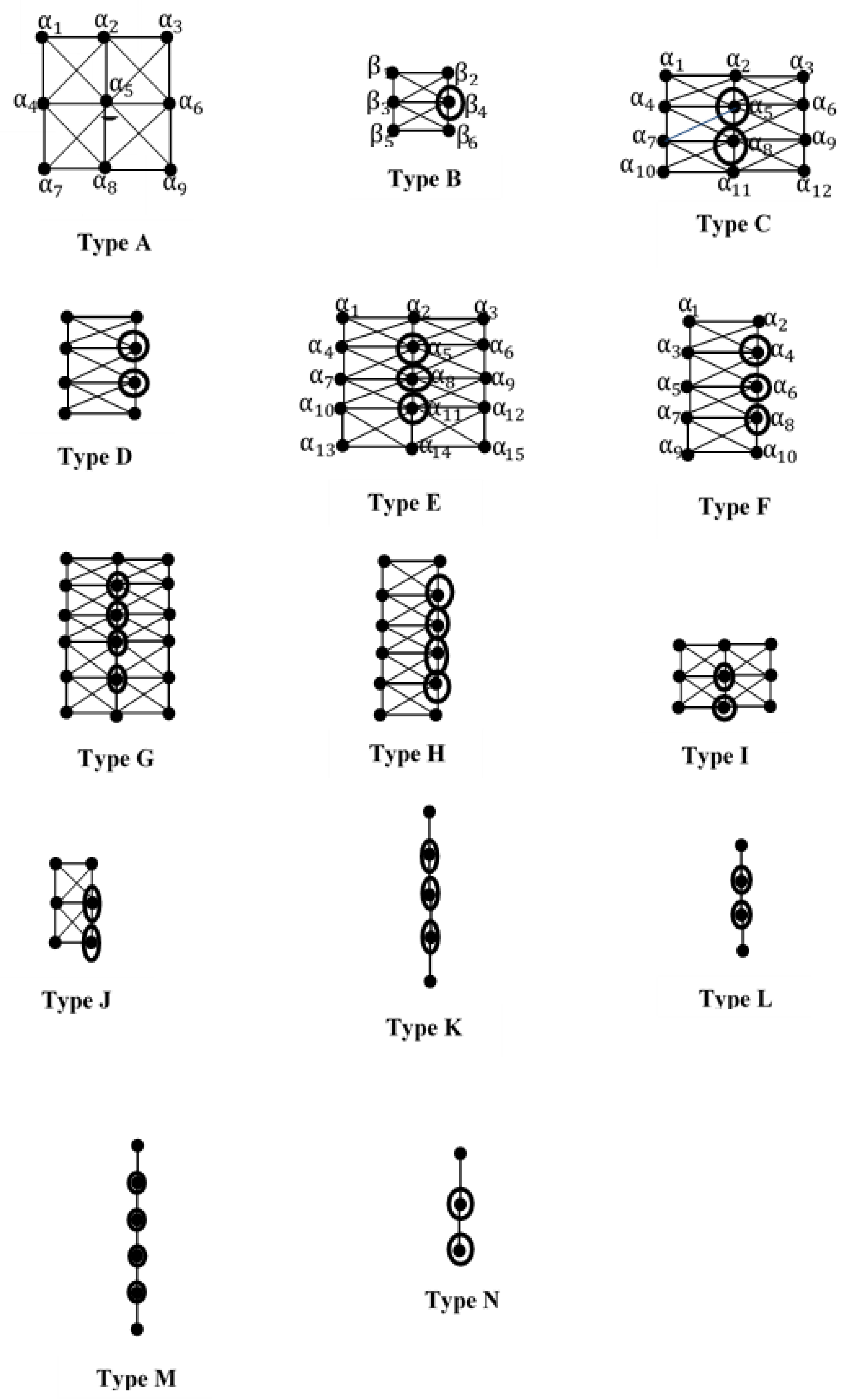
Figure 2.
The graph.
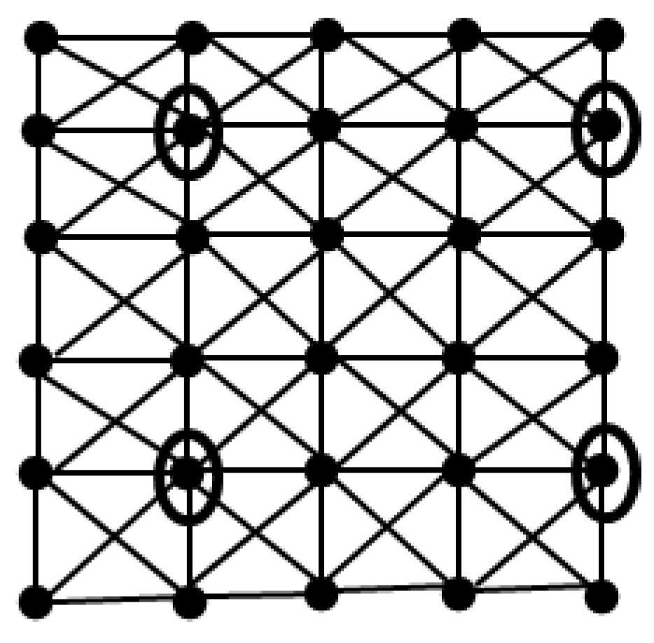
Figure 3.
The graph.
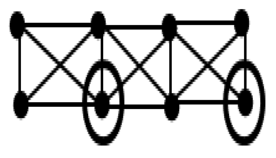
Figure 4.
A 57 mesh or the P5 P7 graph.
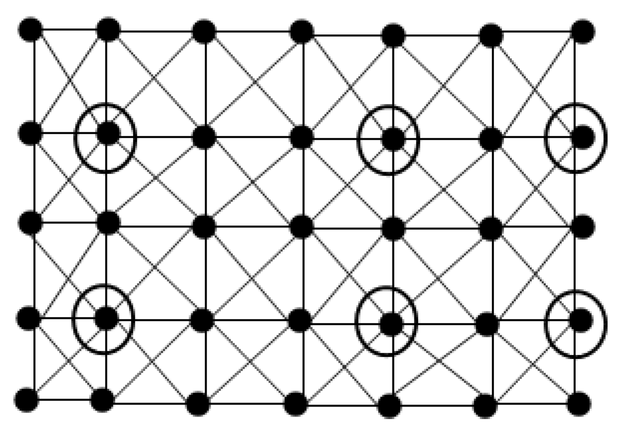
Figure 5.
The P9P5 graph.
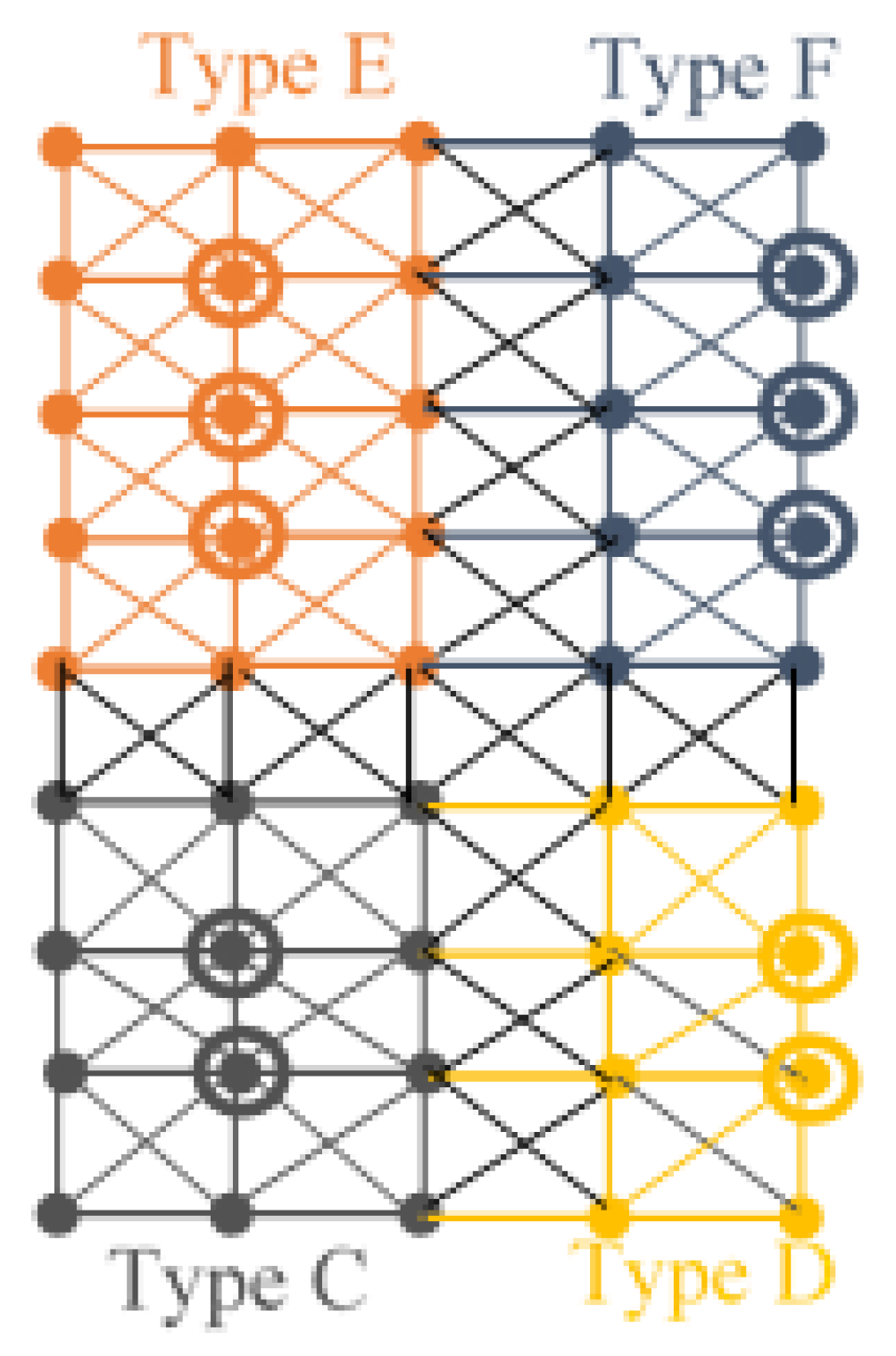
Figure 6.
The graph
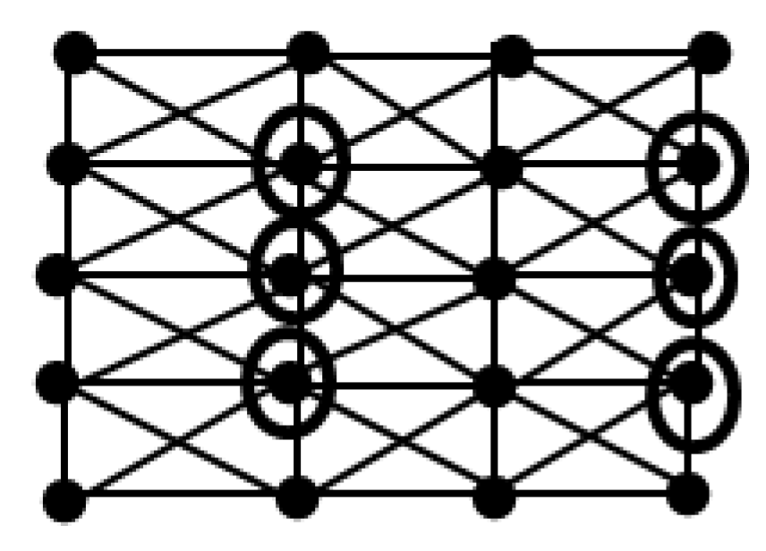
Figure 7.
The graph
Disclaimer/Publisher’s Note: The statements, opinions and data contained in all publications are solely those of the individual author(s) and contributor(s) and not of MDPI and/or the editor(s). MDPI and/or the editor(s) disclaim responsibility for any injury to people or property resulting from any ideas, methods, instructions or products referred to in the content. |
© 2025 by the authors. Licensee MDPI, Basel, Switzerland. This article is an open access article distributed under the terms and conditions of the Creative Commons Attribution (CC BY) license (https://creativecommons.org/licenses/by/4.0/).
Copyright: This open access article is published under a Creative Commons CC BY 4.0 license, which permit the free download, distribution, and reuse, provided that the author and preprint are cited in any reuse.


