Submitted:
11 August 2023
Posted:
14 August 2023
You are already at the latest version
Abstract
The minimum dominating tree (MDT) problem consists of finding a minimum weight sub-graph from an undirected graph, such that each vertex not in this sub-graph is adjacent to at least one of the vertices in it, and the sub-graph is connected without any ring structures. This paper presents a Dual Neighborhoods Search (DNS) algorithm for solving the MDT problem, which integrates several distinguishing features, such as two neighborhoods collaboratively working for optimizing the objective function, a fast neighborhood evaluation method to boost the searching effectiveness, and several diversification techniques to help the searching process jump out of the local optimum trap thus obtaining better solutions. DNS improves the previous best-known results for 4 public benchmark instances while providing competitive results for the remaining ones. Several ingredients of DNS are investigated to demonstrate the importance of the proposed ideas and techniques.
Keywords:
Meta-heuristic
; Dominating tree
; Dual neighborhoods
; Fast neighborhood evaluation
; Optimization
1. Introduction
The minimum dominating tree problem for weighted undirected graphs is to find a dominating tree in a weighted undirected graph such that all vertices in this weighted undirected graph are either in or adjacent to this tree, and the sum of the edge weights of this tree is minimized [1]. Adjacent means that there is an edge between this vertex and at least one vertex in the tree. The minimum dominating tree is a concept in graph theory and one of the important classes of tree structures in graph theory.
A highly related problem, the Minimum Connected Dominating Set (MCDS), has been extensively studied for building routing backbone wireless sensor networks (WSNs) [2,3]. One of the goals of introducing MCDS in WSNs is to minimize energy consumption; if two devices are too far away from each other, they may consume too much power to communicate [4,5]. Using a routing backbone to transmit messages will greatly reduce energy consumption, which increases dramatically as the transmission distance becomes longer [6]. However, some directly connected vertices in MCDS may still be far away from each other because MCDS does not account for distance [7]. Therefore, considering each edge in the routing backbone is more in line with energy consumption purposes [8]. The Minimum Dominating Tree (MDT) problem was first proposed by Zhang et al. [9] for generating a routing backbone that is well adapted to broadcast protocols.
Shin et al. [1] proved that MDT is NP-hard and introduced an approximate framework for solving it. They also provided heuristic algorithms and mixed integer programming (MIP) formulations for the MDT problem. Adasme et al. [10] introduced two other MIP formulations, one based on a tree formulation in the bidirectional counterpart of the input graph, and the other obtained from a generalized spanning tree polyhedron. Adasme et al. [11] proposed a primal dyadic model for the minimum cost dominated tree problem and an effective inequality to improve the linear relaxation. Álvarez-Miranda et al. [12] proposed an precise solution framework that combines a primal-dual heuristic algorithm with a branch-and-cut approach to transform the problem into a Steiner tree problem with additional constraints. Their framework solves most instances in the literature within three hours and proves its optimality.
In recent years, efficient heuristic algorithms for MDT problems have flourished. Sundar and Singh [13] proposed two meta-heuristic algorithms, the Artificial Bee Colony (ABC-DT) algorithm and the Ant Colony Optimization (ACO-DT) algorithm, for the MDT problem. These two algorithms are the first meta-heuristics for the MDT problem and provide better performance than previous algorithms. They also provided 54 randomly generated instances in their work, which are considered challenging instances of the MDT problem and are widely used to evaluate the performance of algorithms for the MDT problem. Based on the latter work, Chaurasia and Singh [14] proposed an evolutionary algorithm with guided mutation (EA/G-MP) for MDT problems. Dražic et al. [15] proposed a variable neighborhood search algorithm for MDT problems. Singh and Sundar [16] proposed another artificial bee colony (ABC-DTP) algorithm for the MDT problem. This new ABC-DTP method differs from ABC-DT in the way it generates initial solutions and in the strategy for determining neighboring solutions. Their experiments show that for the MDT problem, ABC-DTP outperforms all existing problem-specific heuristics and meta-heuristics available in the literature. Hu et al. [17] proposed a hybrid algorithm combining genetic algorithms (GAITLS) and iterative local search to solve the dominated tree problem. Experimental results on classical instances show that the method outperforms existing algorithms. Xiong et al. [18] present a two-level meta-heuristic (TLMH) algorithm for solving the MDT problem with a solution sampling phase and two local search based procedures nested in a hierarchical structure. The results demonstrate the efficiency of the proposed algorithm in terms of solution quality compared with the existing meta-heuristics.
Metaheuristics have been shown to be very effective in solving many challenging real-world problems [19]. However, for some problems, due to the complexity of the problem structure and the large search space, the classical metaheuristic framework fails to produce the desired results [20]. Many researchers have relied on composite neighborhood structures. If properly designed, most composite neighborhood structures have proven successful [21]. These methods include Variable Depth Search (VDS), which searches a large search space through a series of successive simple neighborhood search operations. Although understanding of the basic concepts of VDS algorithms dates back to the 1970s [22], researchers have maintained a sustained enthusiasm for the term [23,24]. For a more detailed survey of VDS, we refer to Ahuja et al. [25,26,27]. Another idea for dealing with complex structural problems is to use a hierarchical meta-trial approach, where several trials are combined in a nested structure. Wu et al. [28] successfully implemented a two-level iterative local search for a network design problem with traffic sparing. According to their analysis, hierarchical metaheuristics must be carefully designed to balance the complexity of the algorithm and its performance. In particular, for the outer framework, keeping it as simple as possible makes the algorithm converge faster. Pop et al. [29] proposed a two-level solution to the generalized minimum spanning tree problem. Carrabs et al. [30] introduced a meta-heuristic algorithm implementing a two-level structure to solve the shortest path problem for all colors. Contreras Bolton and Parada [31] proposed an iterative local search method to solve the generalized minimum spanning tree problem using a two-level solution.
In this paper, we design a meta-heuristic algorithm for two-neighborhood search to solve the MDT problem that uses two neighborhood moves to perform the search and combines a taboo search to escape local optima. The DNS algorithm is described in detail in Section II, the experimental results of the DNS algorithm and comparison with other algorithms are given in Section III, and some comparative experiments within the DNS algorithm are done in Section IV.
2. Dual Neighborhood Search
2.1. Main Framework
The basic idea of our proposed DNS algorithm is to tackle the MDT problem by optimizing the candidate dominating tree weight using a neighborhood search based meta-heuristic with two neighborhood move operators. The search space of DNS consists of all the minimum spanning trees of all the possible dominating sets of the instance graph. The proposed NDS algorithm optimizes the following objective function:
Where stands for the current configuration, i.e., the candidate dominating tree; Notations X and represents the vertex and edge sets of T respectively. Function calculates the number of vertices not dominated by T. Function calculates the weights of the minimum spanning tree of T. And is a constant parameter to balance the importance between and . T is a feasible solution to the minimum dominating tree problem if and only if .
The algorithm primarily comprises several key steps. Firstly, an initial solution is generated, followed by a neighborhood evaluation. Subsequently, the best neighborhood move is selected and executed iteratively. During the iteration, the ever best configuration is recorded. The framework of the algorithm can be represented in pseudo-code as follows:
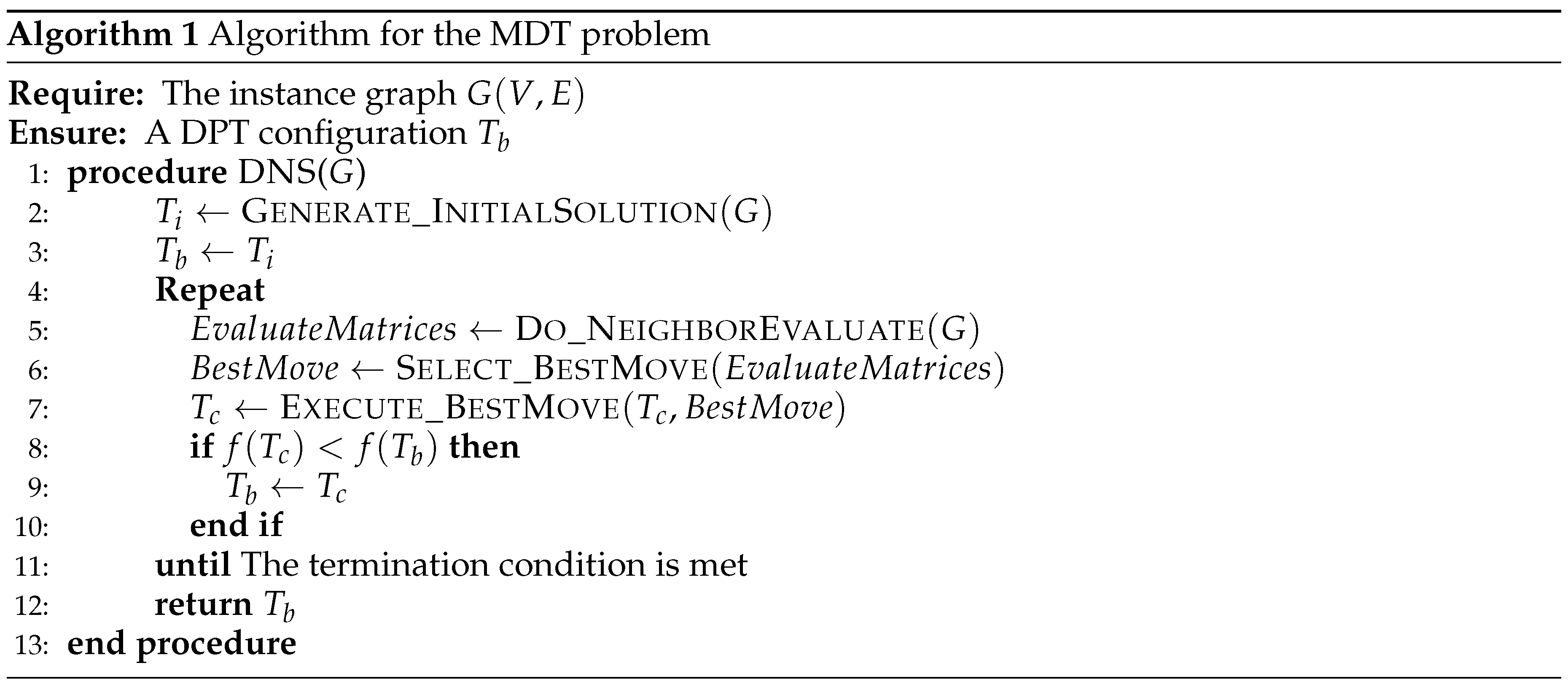
In Algorithm 1, represents the initial configuration, represents the recorded ever best solution, and represents the current configuration. In each iteration, the sub-procedure Do_NeighborEvaluate evaluates all the neighborhood moves in the current configuration. The following two sub-procedure select and execute the best move. The termination condition can be the time or iteration limits.
2.2. Initial Solution Generation
The proposed DNS algorithm uses a feasible dominating tree as the initial configuration. The sub-procedure Generate_InitialSolution generates this initial dominating tree. It first find the minimum spanning tree for the whole graph, and try to trim the tree by removing leaves iteratively until removing one more leave will break the dominancy of the tree. The pseudo-code of this procedure is defined in Algorithm 2.
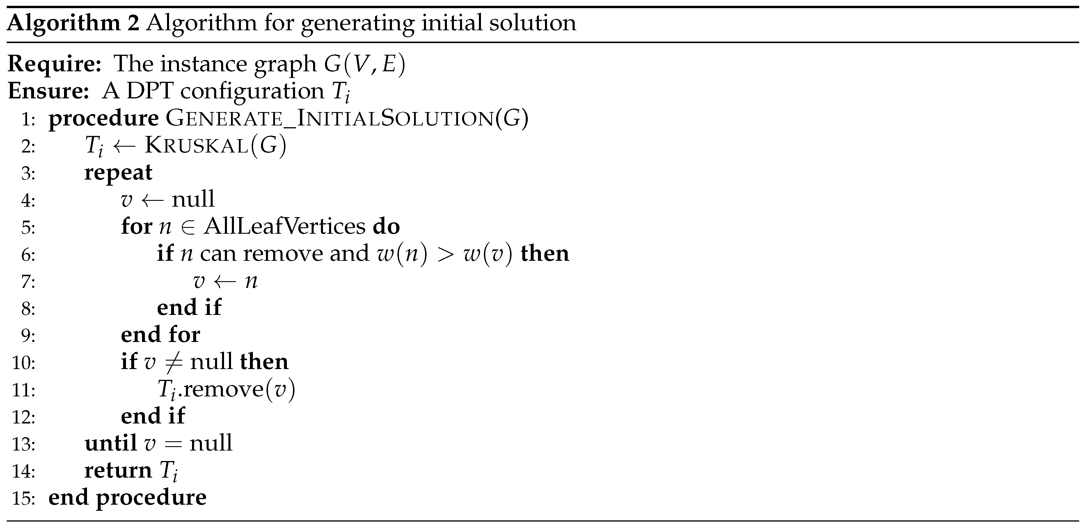
The procedure starts from the minimum spanning tree generated by Kruskal’s algorithm. Then it tries to delete the leaf with the largest edge weight. The process terminates if no more leaf can be deleted. The algorithm returns a feasible dominating tree as the initial configuration. In the following sections, we focus on the meta-heuristic part of the proposed DNS algorithm, i.e., the neighborhood structure as well as its evaluation.
2.3. Definition
For better description, we first define some important concepts and notations used in the proposed DNS algorithm.
- X : the set of vertices in the current dominator tree.
- : the set of vertices dominated by X and not in X.
-
: An array of the number of un-dominated vertices, the length of the array is the number of graph vertices.denotes the number of vertices not dominated by the new X if move i from X to (or from to X).
-
: array of minimum spanning tree weights for X. The length of the array is the number of graph vertices.denotes the weight of the new minimum spanning tree of X if move i from X to (or from to X).
The following example illustrates how and are calculated.
As shown in the Figure 1, the current dominating tree is containing two vertices, B and D. Therefore, . The vertices dominated by X are A, C, and E. Thus, . We correspond the vertices A, B, C, D, and E to the array subscripts 0, 1, 2, 3, and 4, respectively. To evaluate the neighborhood moves, the algorithm takes vertex A out and puts it in the set of the other side. The number of vertices that are not dominated by the new X after this move is 0, thus is assigned to 0. The weight of the new minimum spanning tree of X is 13, thus is assigned to 13. After evaluating all the neighborhood moves, the resulting arrays are and . and are used to evaluate the neighborhood moves.
2.4. Neighborhood move and Evaluation
There are two kinds of neighborhood moves in DNS algorithm, one is to take out one vertex in X and put it into , and the other one is to take out one vertex in and put it into X. In each iteration, the best neighborhood move is selected and performed among all the two kinds of neighborhood moves. There are two criteria to evaluate the quality of the moves, one is the dominance and the other is the weight of the dominating tree. The pseudo-code for neighborhood evaluation is described in Algorithm 3.
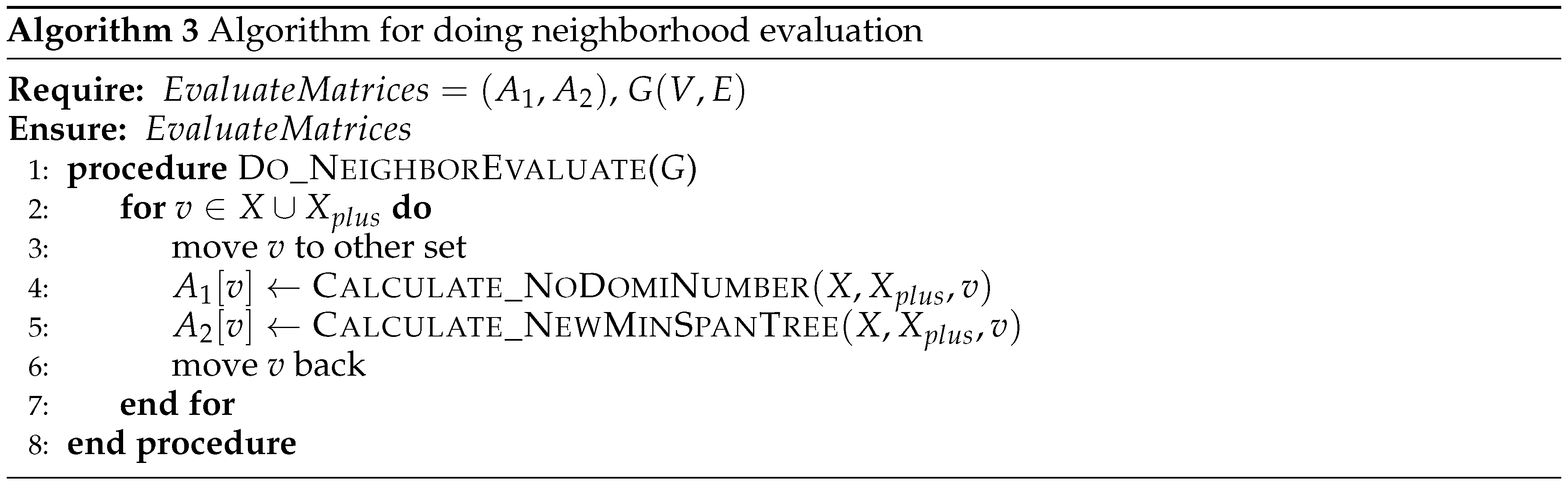
The evaluation is done by trying to move each vertex to the other set, then calculate the and values. Based on these two arrays, the best move is selected as described in Algorithm 4.
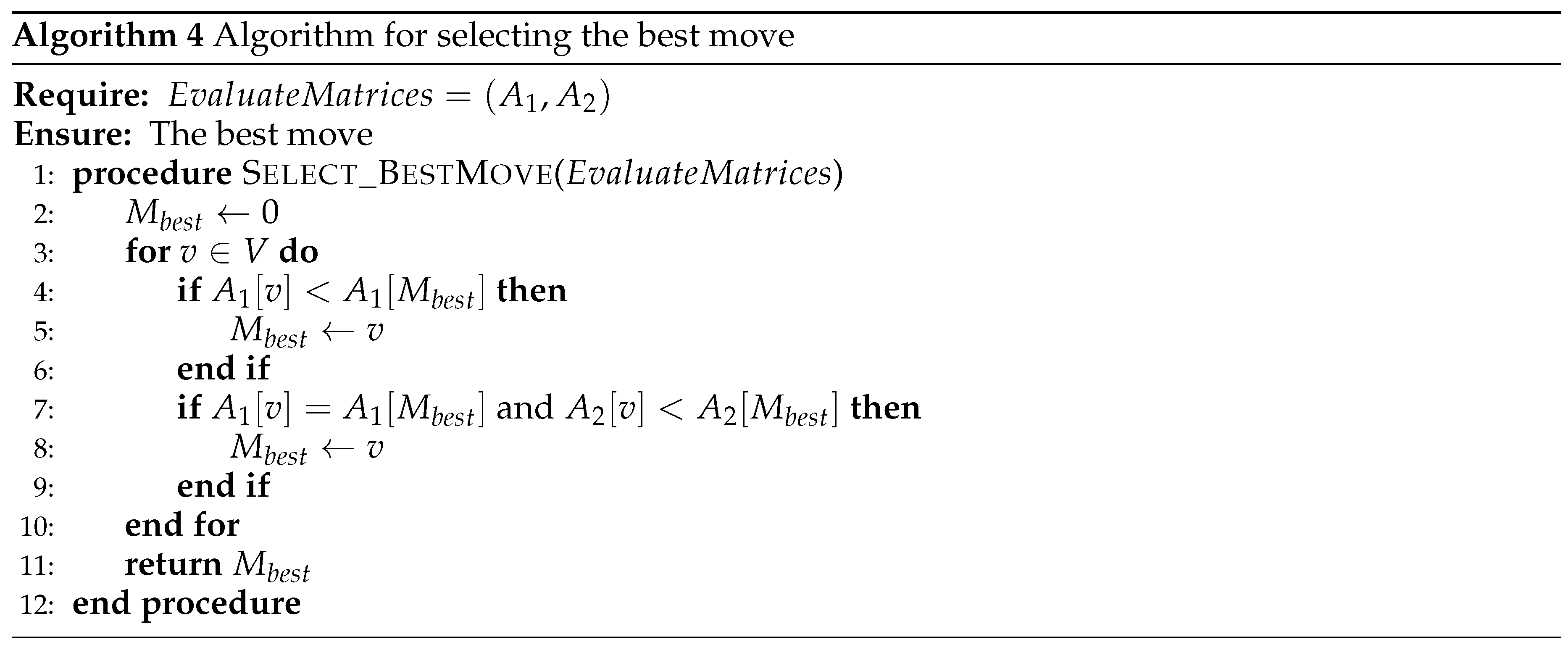
Procedure Select_BestMove picks the move with the smallest and , higher priority for . Then, the best move selected is performed by Algorithm 5.
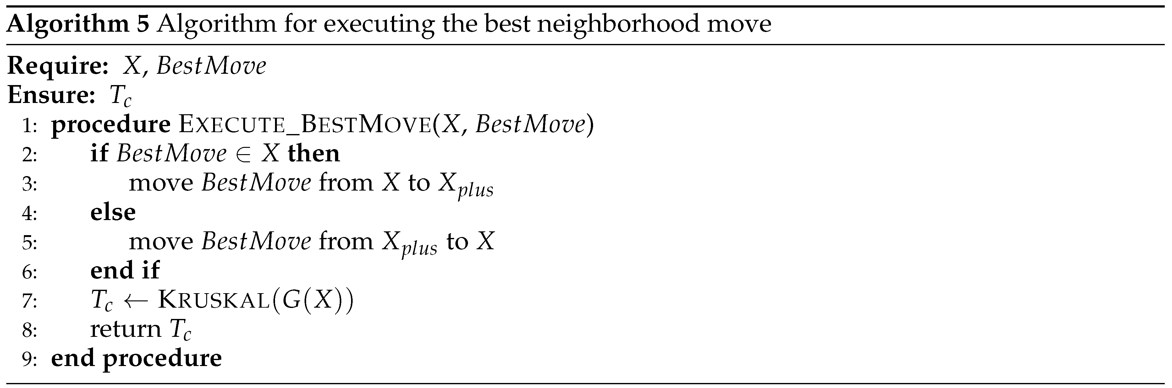
Procedure Execute_BestMove moves the selected vertex to if it is in X, and vice versa. After the move, the minimum spanning tree of is calculated using Kruskal’s algorithm and assigned to . The following example illustrates how the best move is evaluated and performed.
As shown in Figure 2, the current domination tree is , , . To evaluate vertex A, we first move it from to X, then X becomes . The number of vertices that are not dominated by the new X at this point is 0, thus . The minimum spanning tree weight of is 13, thus . We then move A back to its original set. The evaluation for A is done. The B, C, D, and E are evaluated sequentially by the same process. After the evaluation for each vertex, and .
Then we pick the best neighborhood move, finding the minimum value from and , prior to . There are 3 minimum values in , corresponding to A, C, and E. Then we compare the value of these three vertices in , the minimum value is 3, corresponding to vertex E. Therefore, the best vertex is E, and the best neighboring move is to move E. After the move, the new . We calculate the minimum spanning tree of the new X. The new minimum spanning tree is with a weight of 3.
2.5. Fast Neighborhood Evaluation
In order to improve the efficiency of the algorithm, this paper proposes a method to dynamically update the neighborhood evaluation matrices , .
2.5.1. Fast evaluation for
The number of un-dominated vertices may increase or remain unchanged when vertices are removed from X to . The newly added un-dominated vertices must be originally in the set and connected to the moved vertex. Since the number of un-dominated vertices is zero throughout the algorithm, we can count the newly introduced un-dominated vertices by counting the vertices in , which the moved vertex is its only connection to X.
When we move vertices from to X, the number of un-dominated vertices may decrease or remain the same. Because X is dominated throughout the algorithm, the number of un-dominated vertices after this kind of moves is still 0. The above observation can be utilized to dynamically compute without having to traverse the entire graph. The formula is as follows:
2.5.2. Fast evaluation for
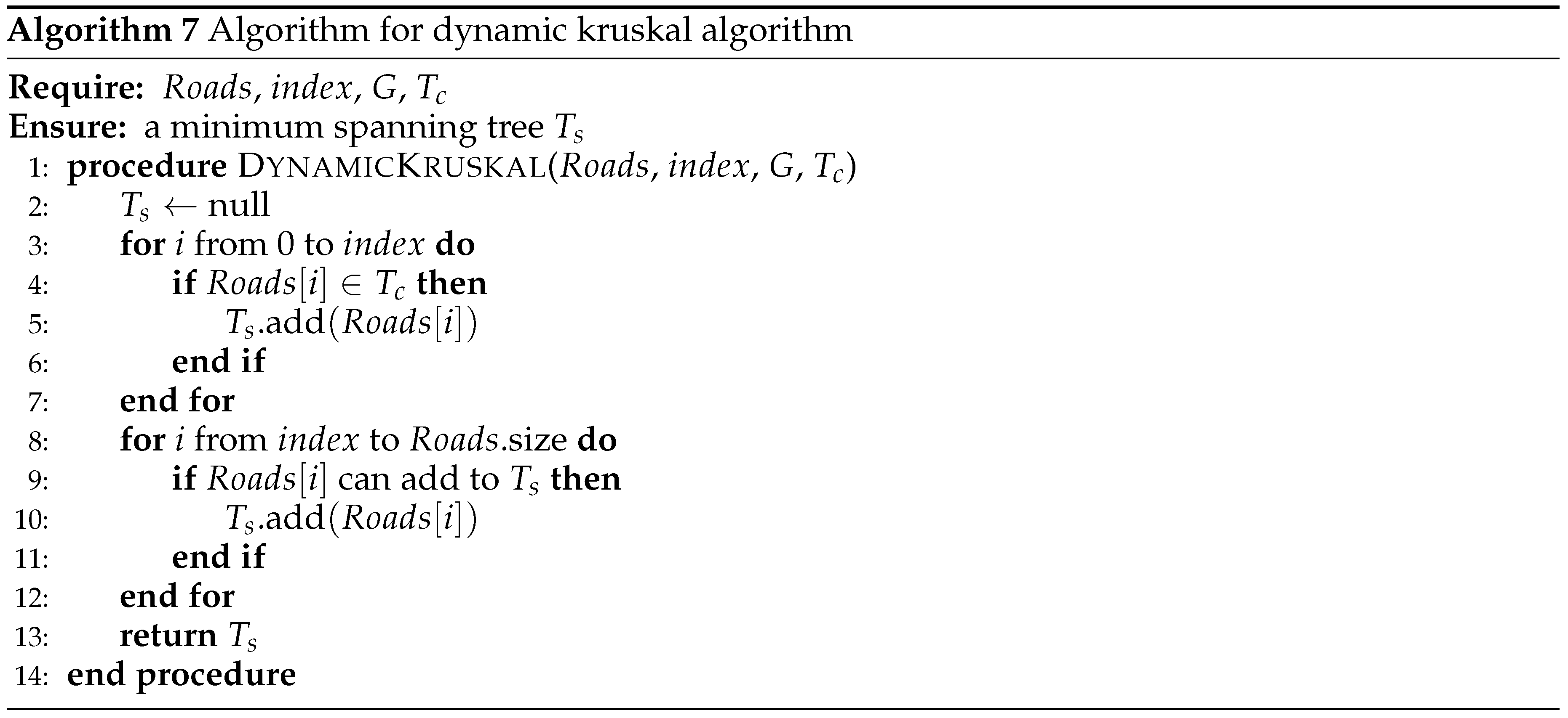
For , we use a dynamic Kruskal’s algorithm. The algorithm dynamically maintains a set , which is the set of edges contained in the subgraph , i.e., the set of edges whose two vertices are in X. The set is sorted from smallest to largest by the weights of the edges. When a X to move is performed, the edges connecting to the moved vertex and X are deleted from the set. Similarly, when a to X move is performed, the edges connecting to the moved vertex and X are inserted to the set. Note that, edges should be inserted into the appropriate position in to guarantee that it is sorted. The dynamic Kruskal’s algorithm then assumes that the edges before the deletion or insertion position are sure to be in the new minimum spanning tree, then start the normal procedure from that position. The pseudo-code for dynamic Kruskal’s algorithm is described in Algorithm 6 and 7.
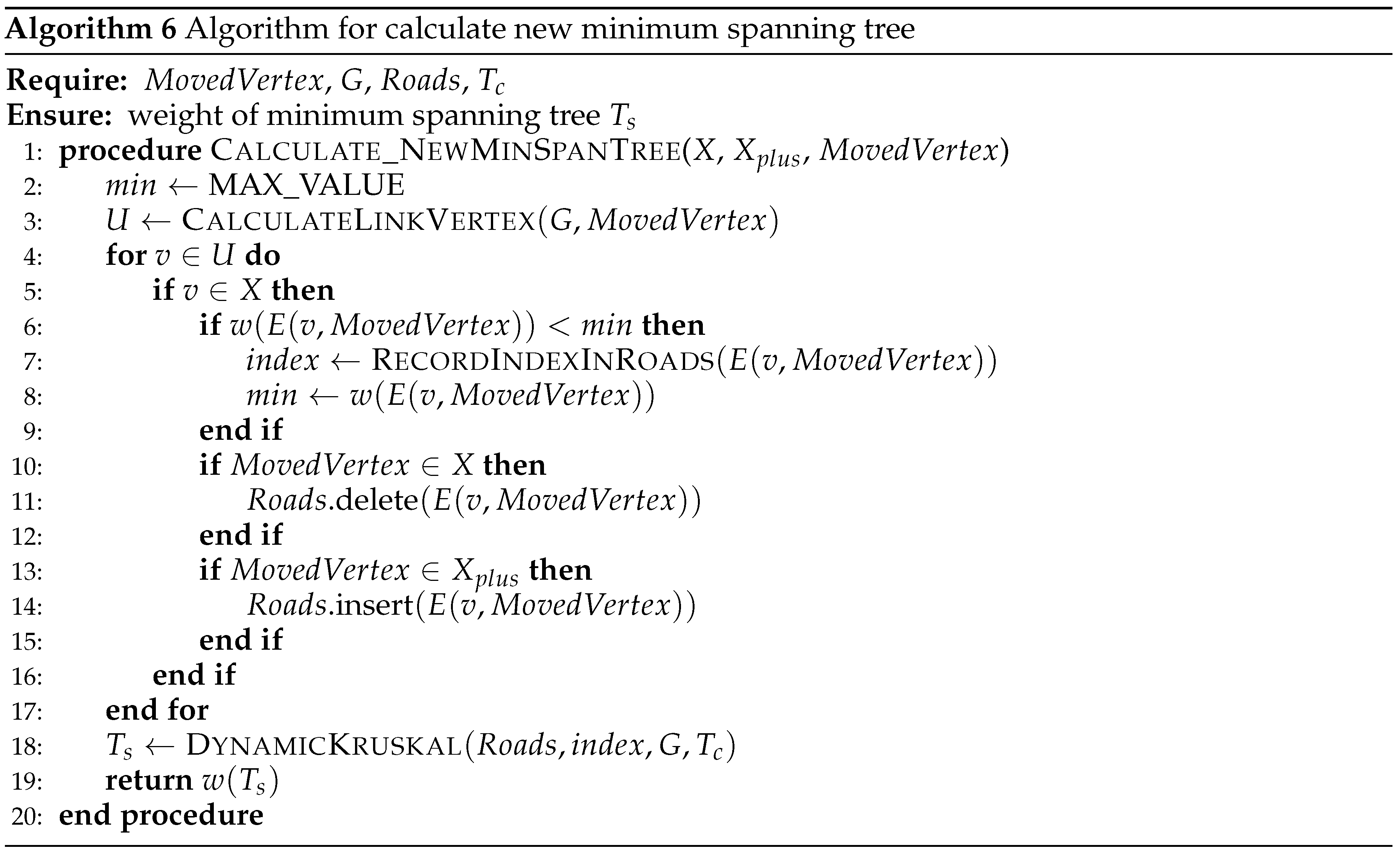
In Algorithm 6, The notate represents the edge connecting vertices a and b, is the original minimum spanning tree, i.e., the entire algorithm of the current solution. The main job for this procedure is to update the set. And the Algorithm 7 calculates the spanning tree dynamically according to .
The following example illustrates the above procedures:
As shown in Figure 3, the original tree is , currently, , , , and the weights of the edges . Let’s evaluate the move of vertex E from to X. After the move , . Since E was originally in , . The new edge added after the move is the edge with weights . Then we insert these two edges into the appropriate position in according to their weights from smallest to largest in , and the corresponding . We only need to start from position of to determine the new minimum spanning tree. The edges before must be in the new minimum spanning tree. The evaluated minimum spanning tree is with weight 12, thus .
2.6. Tabu strategy and aspiration mechanism
The proposed DNS algorithm implements tabu strategy. The vertex is prohibited to be moved again within a tenure once it is moved. The tabu strategy is implemented to both kinds of moves in the algorithm. Since there is no intersection of X and , only one taboo table is needed. We denote the tabu tenure of the move from to X as and the move from X to as . These two tabu tenures are set to the number of vertices in X and , respectively, thus implementing dynamic tabu tenures in this way. This tabu strategy improves the accuracy and efficiency makes the algorithm to jump out of the local optimum more easily.
In order to avoid missing some good solutions, an aspiration strategy is introduced. If one tabu move may improve the ever best solution, the searching process breaks its tabu status and selects it as a candidate best move.
Note that we do not describe the details of how the tabu and aspiration is implemented in the previous pseudo-codes to give a clearer layout for better understanding. For more details of tabu we recommend readers to the literature [32].
2.7. Perturbation Strategy
In order to further improve the quality of the solution, the proposed DNS algorithm implements a perturbation strategy. The specific perturbation is to move some vertices from to X randomly. The algorithm set a parameter as the perturbation period. When the number of iterations reaches the perturbation period a perturbation will be triggered, and the number of iterations will be cleared to zero if the ever best solution is updated within this period. There are another two parameters, the perturbation amplitude and the perturbation tabu tenure. The perturbation amplitude is the number of vertices taken out from in the perturbation. The perturbation tabu tenure is the tabu tenure used during the perturbation period. In addition, after a certain number of small perturbations, a larger perturbation needs to be triggered to give a larger spatial span to the search process. The larger perturbation is implemented by moving one-third of the vertices from to X randomly.
3. Algorithm Experimentation
3.1. Datasets and Experimental Protocols
The experiments are carried out on the following two data sets:
Both datasets are randomly generated and can be downloaded online or obtained from the authors. The DNS algorithm is implemented in Java (JDK17) and tested on a desktop computer equipped with an Intel® Xeon® W-2235 CPU @3.80GHz, with 16.0GB of RAM.
3.2. Calibration
This section we conduct experiments to fix the value of key parameters of DNS algorithm:
- Parameter , the first perturbation period. Values from 14 to 17 are tested.
- Parameter , the perturbation amplitude. Values from 7 to 12 are tested.
- Parameter , The tabu length of the neighborhood move of taking a vertex from and putting it into X during perturbation. Values from 1 to 2 are tested.
- Parameter , The tabu length of the neighborhood move of taking a vertex from X and putting it into during perturbation. Values from 3 to 8 are tested.
We select 13 representative instances to tackle the calibration experiments. Representatives are instances 200-400-1, 200-600-1, 300-600-1 and 300-1000-1 In DTP; instances 300-1, 400-1 and 500-1 respectively in Range100, Range125 and Range150. The experiment is done as following steps: First, roughly experiment with parameter combinations to select better parameter combinations. Then for each set of parameters, run these 13 instances in sequence. Each instance is run five times with different random seeds for 300 seconds each time. We compare the gap rates for each parameter setting. The gap is calculated as:
, where is the average result obtained and is the known best objective. Table 1 shows the result for the calibration experiment.
According to the experimental data, the minimum total rate is 0.075, corresponding to of 15, of 8, of 1, and of 4. In the following experiment, we set the parameters of the algorithm to this setting. Note that this experiment does not guarantee the optimal values of the parameters and the optimal scheme may vary from one benchmark to another. It can also be seen that for different parameter combinations, the rate is small, indicating the robustness of the algorithm.
3.3. Comparison on DTP Data Set
In this section, we compare the proposed DNS algorithm with other methods in the literature on DTP data set. There are two DTP datasets: dtp_large and dtp_small. Since all algorithms can obtain the best results for dtp_small with little difference in speed, only the experimental results for dtp_large are shown here. The compared algorithms are TLMH, VNS, and GAITLS algorithms. For each instance, 10 runs with different random seeds are made, each lasting 1000 seconds. The best, average objective values, and average time are recorded for each instance. The experimental results and comparisons are shown in Table 2. Bolded numbers represent that the current best value has been obtained and the results are not worse than other algorithms. The start marks represent that DNS algorithm updates the best objective in the literature.
From Table 2, it can be seen that this algorithm runs most instances to the best value, and those that do not reach the optimal value are also very close to it. The overall best values are slightly worse than the TLMH algorithm but better than the VNS and GAITLS algorithms. The overall average of this algorithm outperforms other algorithms, demonstrating its stability and faster speed. It also improves the best solution for two instances.
3.4. Range Dataset Experiments
In this section, the widely used Range dataset with 54 instances is tested and compared with the TLMH, ACO-DT, EA/G-MP, and ABC-DTP algorithms. The experimental results of these algorithms compared in this paper are the best results obtained using the best parameters in the original literature. In this section, this algorithm is run 10 times for each dataset with the previously measured best parameters and different random seeds. Each run lasts 1000 seconds and the best, average objective values, and average time are calculated. The results and comparisons are shown in Table 3, Table 4 and Table 5:
==layoutwidth=297mm,layoutheight=210 mm, left=2.7cm,right=2.7cm,top=1.8cm,bottom=1.5cm, includehead,includefoot [LO,RE]0cm [RO,LE]0cm
==This algorithm obtains best solutions for most instances in the Range dataset, and those that are not optimal are close to the optimal solution. It updates the best solution for two instances and outperforms the TLMH algorithm in speed.
4. Analysis and Discussion
4.1. The Importance of the Initial Solution
A procedure for generating the initial solution was proposed in the previous chapter. To see the effect of this procedure, experiments were conducted on it in this section, where 18 instances of Range150 were tested. The objective value obtained by this procedure were compared with both the minimum spanning tree weights and the known best objective value to see how much this procedure improves on the initial solution and how close this initial solution is to the minimum domination tree. The experimental results are shown in Table 6.
In Table 6, represents the minimum spanning tree, represents the objective value obtained from the initialization procedure, represents the known best objective value. From the results, it can be seen that using the initialization procedure to obtain a domination tree as the initial solution improves significantly over using the minimum spanning tree as the initial solution. The weight of this initial domination tree is relatively close to that of the minimum domination tree, allowing the algorithm to converge quickly to a near-optimal solution at the very beginning. To verify this improvement, this paper also uses the minimum spanning tree of graph as an initial solution and conducts experiments on Range150 for comparison. This method is denoted as DNS-ms. The experimental results are in Table 7.
The experimental results show that DNS outperforms the DNS-ms algorithm in terms of best, average objective values, and speed, indicating that the initial solution proposed in this paper improves the efficiency of the algorithm. It can also be seen that there is not much difference between the best and average values obtained by DNS and DNS-ms, demonstrating the robustness of the local search procedure of DNS algorithm.
4.2. The Importance of the Fast Neighborhood Evaluation
The proposed DNS algorithm uses a fast neighborhood evaluation technique. To verify its effectiveness, an experiment was conducted to test the time taken to reach the same result for 18 instances of Range150 with and without fast neighborhood evaluation. In this experiment, the perturbation is disabled while only tabu mechanism is enabled. The best objective value that can be reached at complete convergence is tested in advance for each instance and used as the target result. The random seed is fixed for each instance because the difference in speed is only due to using fast neighborhood evaluation. The program runs until it reaches the target result, and the time taken by each instance to reach the target result under these two methods is recorded separately. The results are shown in Table 8, where Method 1 represents the version without fast neighborhood evaluation and Method 2 represents the version with fast neighborhood evaluation:
From Table 8, it can be seen that the version using fast neighborhood evaluation significantly improves speed compared to the version without it, verifying the effectiveness of fast neighborhood evaluation. To observe the convergence of these two methods, scatter plots are generated by outputting the weights and corresponding times after each update. The convergence curves of some instances are shown in Figure 4, where NDNU represents the method without fast neighborhood evaluation and DNU represents the method with the fast neighborhood evaluation.
From Figure 4, it can be seen that the version using fast neighborhood evaluation converges to the target value more quickly. For the version without the fast neighborhood evaluation, the curve is slower and takes longer to converge to the same objective value.
4.3. Importance of the Perturbation
The proposed DNS algorithm also implements a perturbation strategy. In this section the effectiveness of this strategy is verified through experiments by testing the version with and without this strategy, for 18 instances in Range150. Each instance is run 5 times with different random seeds, with a time limit of 1000 seconds, and the results of the experiments are shown in Table 9:
From Table 9, it can be seen that better solutions can be obtained by the version using the perturbation strategy, especially in some larger instances, verifying the effectiveness of this strategy.
5. Conclusion
In this paper, a dual-neighborhood search algorithm is proposed to solve the minimum dominating tree problem. In order to improve the efficiency of the algorithm, a fast neighborhood evaluation method is proposed, in which the method of dynamically generating the minimum spanning tree from the sub-graph deduced from the dominating set. The tabu and the perturbation mechanisms help the algorithm jump out of the local optimum trap, thus obtaining better solutions. The DNS algorithm is demonstrated to be highly effective in tests on a collection of widely used benchmark instances where it is compared with the algorithms in the literature. Out of 72 public instances, DNS improves the best result on 4 problems while being competitive on the remaining ones with less computational time. Although the techniques proposed in this paper are specific to the minimum dominating tree problem, most of these ideas can be applied to other combinatorial optimization problems. For example, the dynamic spanning tree calculation used in the fast neighborhood evaluation can be used in problems with spanning tree structures. And the collaboration of two neighborhood structures can be also introduced to other relevant optimization problems. Finally, it is interesting to test the proposed ideas in other meta-heuristic frameworks with other optimization problems.
References
- Shin, I.; Shen, Y.; Thai, M.T. On approximation of dominating tree in wireless sensor networks. Optimization Letters 2010, 4, 393–403. [Google Scholar] [CrossRef]
- Wu, X.; Lü, Z.; Galinier, P. Restricted swap-based neighborhood search for the minimum connected dominating set problem. Networks 2017, 69, 222–236. [Google Scholar] [CrossRef]
- Li, R.; Hu, S.; Gao, J.; Zhou, Y.; Wang, Y.; Yin, M. GRASP for connected dominating set problems. Neural Computing and Applications 2017, 28, 1059–1067. [Google Scholar] [CrossRef]
- Li, R.; Hu, S.; Liu, H.; Li, R.; Ouyang, D.; Yin, M. Multi-start local search algorithm for the minimum connected dominating set problems. Mathematics 2019, 7, 1173. [Google Scholar] [CrossRef]
- Bouamama, S.; Blum, C.; Fages, J.G. An algorithm based on ant colony optimization for the minimum connected dominating set problem. Applied Soft Computing 2019, 80, 672–686. [Google Scholar] [CrossRef]
- Chinnasamy, A.; Sivakumar, B.; Selvakumari, P.; Suresh, A. Minimum connected dominating set based RSU allocation for smartCloud vehicles in VANET. Cluster Computing 2019, 22, 12795–12804. [Google Scholar] [CrossRef]
- Hedar, A.R.; Ismail, R.; El-Sayed, G.A.; Khayyat, K.M.J. Two meta-heuristics designed to solve the minimum connected dominating set problem for wireless networks design and management. Journal of Network and Systems Management 2019, 27, 647–687. [Google Scholar] [CrossRef]
- Li, B.; Zhang, X.; Cai, S.; Lin, J.; Wang, Y.; Blum, C. Nucds: An efficient local search algorithm for minimum connected dominating set. In Proceedings of the Proceedings of the Twenty-Ninth International Conference on International Joint Conferences on Artificial Intelligence, 2021; pp. 1503–1510.
- Zhang, N.; Shin, I.; Li, B.; Boyaci, C.; Tiwari, R.; Thai, M.T. New approximation for minimum-weight routing backbone in wireless sensor network. In Proceedings of the Wireless Algorithms, Systems and Applications: Third International Conference, WASA 2008, Dallas, TX, USA, October 26-28, 2008. Proceedings 3. Springer, 2008; pp. 96–108.
- Adasme, P.; Andrade, R.; Leung, J.; Lisser, A. Models for minimum cost dominating trees. Electronic Notes in Discrete Mathematics 2016, 52, 101–107. [Google Scholar] [CrossRef]
- Adasme, P.; Andrade, R.; Leung, J.; Lisser, A. Improved solution strategies for dominating trees. Expert Systems with Applications 2018, 100, 30–40. [Google Scholar] [CrossRef]
- Álvarez-Miranda, E.; Luipersbeck, M.; Sinnl, M. An exact solution framework for the minimum cost dominating tree problem. Optimization Letters 2018, 12, 1669–1681. [Google Scholar] [CrossRef]
- Sundar, S.; Singh, A. New heuristic approaches for the dominating tree problem. Applied Soft Computing 2013, 13, 4695–4703. [Google Scholar] [CrossRef]
- Chaurasia, S.N.; Singh, A. A hybrid heuristic for dominating tree problem. Soft Computing 2016, 20, 377–397. [Google Scholar] [CrossRef]
- Dražić, Z.; Čangalović, M.; Kovačević-Vujčić, V. A metaheuristic approach to the dominating tree problem. Optimization Letters 2017, 11, 1155–1167. [Google Scholar] [CrossRef]
- Singh, K.; Sundar, S. Two new heuristics for the dominating tree problem. Applied Intelligence 2018, 48, 2247–2267. [Google Scholar] [CrossRef]
- Hu, S.; Liu, H.; Wu, X.; Li, R.; Zhou, J.; Wang, J. A hybrid framework combining genetic algorithm with iterated local search for the dominating tree problem. Mathematics 2019, 7, 359. [Google Scholar] [CrossRef]
- Xiong, C.; Liu, H.; Wu, X.; Deng, N. A two-level meta-heuristic approach for the minimum dominating tree problem. Frontiers of Computer Science 2023, 17, 171406. [Google Scholar] [CrossRef]
- Yang, W.; Ke, L. An improved fireworks algorithm for the capacitated vehicle routing problem. Frontiers of Computer Science 2019, 13, 552–564. [Google Scholar] [CrossRef]
- Hou, N.; He, F.; Zhou, Y.; Chen, Y. An efficient GPU-based parallel tabu search algorithm for hardware/software co-design. Frontiers of Computer Science 2020, 14, 1–18. [Google Scholar] [CrossRef]
- Hao, X.; Liu, J.; Zhang, Y.; Sanga, G. Mathematical model and simulated annealing algorithm for Chinese high school timetabling problems under the new curriculum innovation. Frontiers of Computer Science 2021, 15, 1–11. [Google Scholar] [CrossRef]
- Lin, S.; Kernighan, B.W. An effective heuristic algorithm for the traveling-salesman problem. Operations research 1973, 21, 498–516. [Google Scholar] [CrossRef]
- Glover, F. Ejection chains, reference structures and alternating path methods for traveling salesman problems. Discrete Applied Mathematics 1996, 65, 223–253. [Google Scholar] [CrossRef]
- Yagiura, M.; Yamaguchi, T.; Ibaraki, T. A variable depth search algorithm with branching search for the generalized assignment problem. Optimization Methods and Software 1998, 10, 419–441. [Google Scholar] [CrossRef]
- Ahuja, R.K.; Ergun, Ö.; Orlin, J.B.; Punnen, A.P. A survey of very large-scale neighborhood search techniques. Discrete Applied Mathematics 2002, 123, 75–102. [Google Scholar] [CrossRef]
- Santos, L.F.M.; Iwayama, R.S.; Cavalcanti, L.B.; Turi, L.M.; de Souza Morais, F.E.; Mormilho, G.; Cunha, C.B. A variable neighborhood search algorithm for the bin packing problem with compatible categories. Expert Systems with Applications 2019, 124, 209–225. [Google Scholar] [CrossRef]
- Wu, X.; Xiong, C.; Deng, N.; Xia, D. A variable depth neighborhood search algorithm for the Min–Max Arc Crossing Problem. Computers & Operations Research 2021, 134, 105403. [Google Scholar]
- Wu, X.; Lü, Z.; Guo, Q.; Ye, T. Two-level iterated local search for WDM network design problem with traffic grooming. Applied Soft Computing 2015, 37, 715–724. [Google Scholar] [CrossRef]
- Pop, P.C.; Matei, O.; Sabo, C.; Petrovan, A. A two-level solution approach for solving the generalized minimum spanning tree problem. European Journal of Operational Research 2018, 265, 478–487. [Google Scholar] [CrossRef]
- Carrabs, F.; Cerulli, R.; Pentangelo, R.; Raiconi, A. A two-level metaheuristic for the all colors shortest path problem. Computational Optimization and Applications 2018, 71, 525–551. [Google Scholar] [CrossRef]
- Contreras-Bolton, C.; Parada, V. An effective two-level solution approach for the prize-collecting generalized minimum spanning tree problem by iterated local search. International Transactions in Operational Research 2021, 28, 1190–1212. [Google Scholar] [CrossRef]
- Glover, F.; Laguna, M. Tabu search; Springer, 1998.
Figure 1.
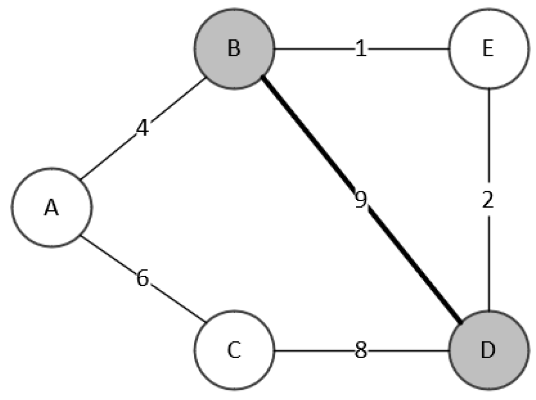
Figure 2.
Move to
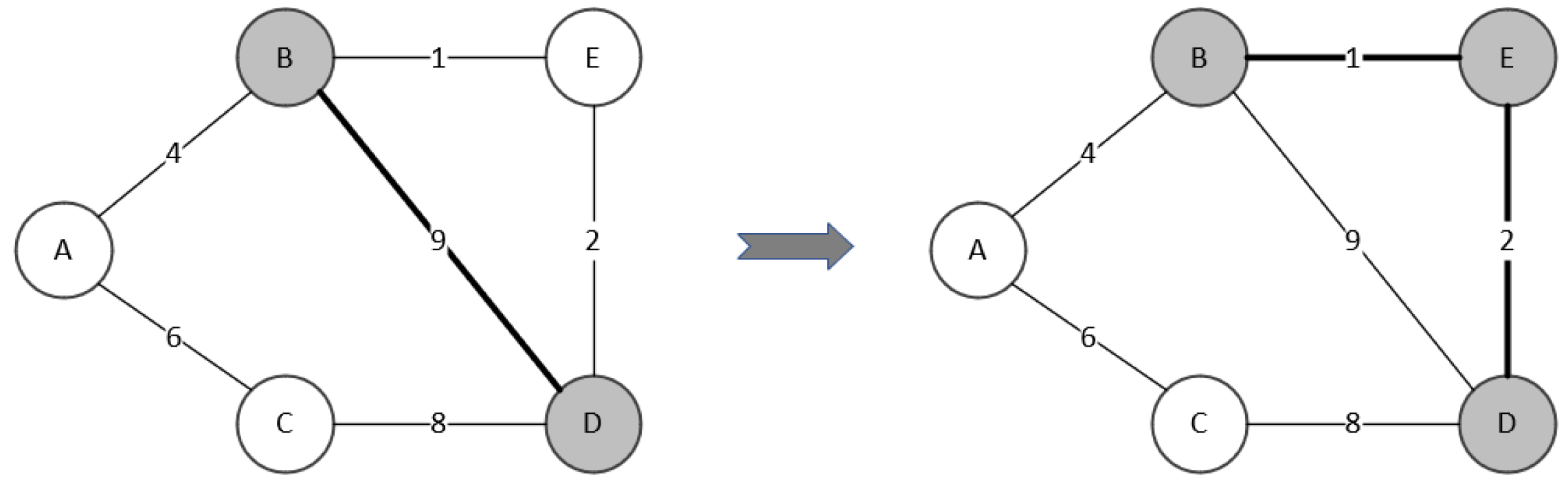
Figure 3.
to
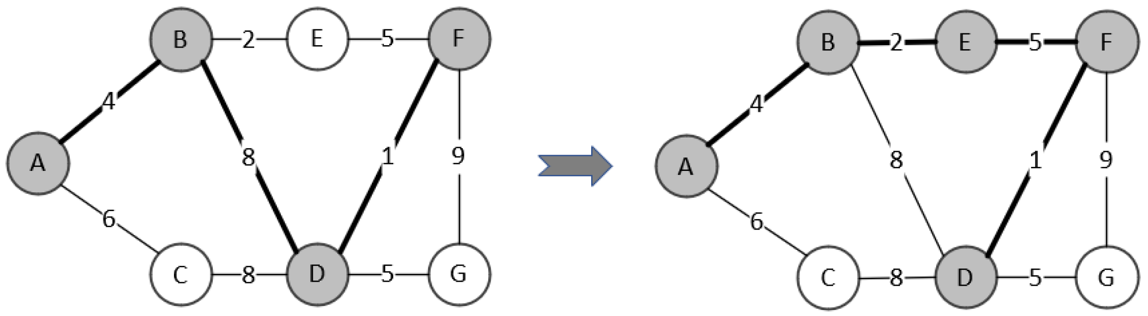
Figure 4.
Fast neighborhood evaluation scatter plot
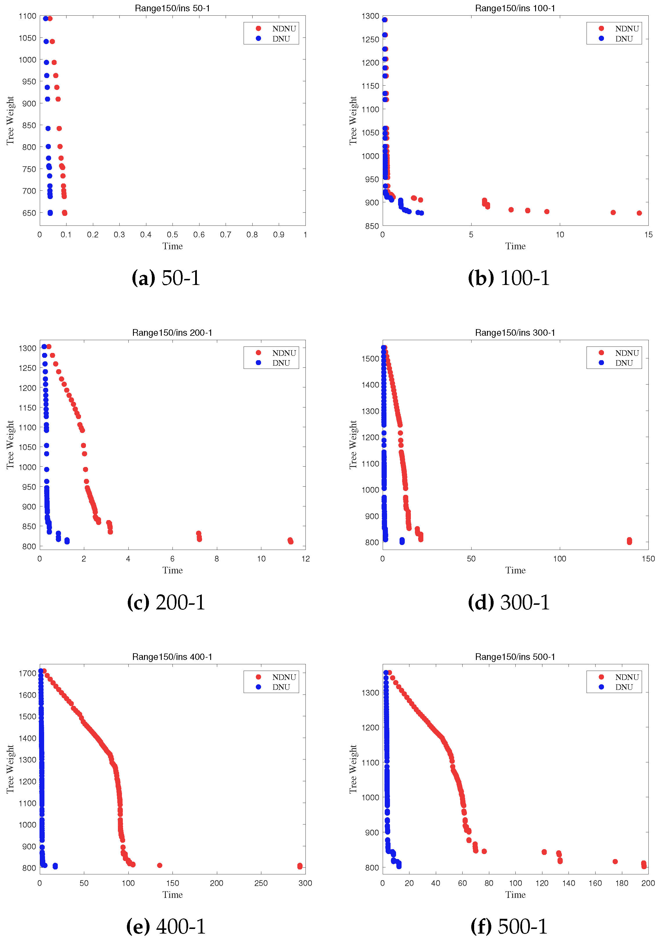

Table 1.
Experimental results of parameter testing for DNS
| DisturbPeriod | DisturbLevel | DisturbTL_1 | DisturbTL_2 | TotalGap | AverageTime |
|---|---|---|---|---|---|
| 14 | 7 | 1 | 3 | 0.083 | 1959 |
| 14 | 7 | 1 | 4 | 0.082 | 1696 |
| 14 | 7 | 1 | 5 | 0.083 | 1806 |
| 14 | 8 | 1 | 3 | 0.093 | 1803 |
| 14 | 8 | 1 | 4 | 0.077 | 1776 |
| 14 | 8 | 1 | 5 | 0.080 | 1733 |
| 14 | 9 | 1 | 3 | 0.093 | 1910 |
| 14 | 9 | 1 | 4 | 0.090 | 1985 |
| 14 | 9 | 1 | 5 | 0.095 | 2084 |
| 15 | 8 | 1 | 4 | 0.075 | 1822 |
| 15 | 8 | 1 | 5 | 0.086 | 1768 |
| 15 | 8 | 1 | 6 | 0.083 | 1854 |
| 15 | 9 | 1 | 4 | 0.096 | 1956 |
| 15 | 9 | 1 | 5 | 0.095 | 1772 |
| 15 | 9 | 1 | 6 | 0.107 | 1835 |
| 15 | 10 | 1 | 4 | 0.077 | 1945 |
| 15 | 10 | 1 | 5 | 0.093 | 1955 |
| 15 | 10 | 1 | 6 | 0.096 | 1906 |
| 16 | 9 | 2 | 5 | 0.097 | 1930 |
| 16 | 9 | 2 | 6 | 0.110 | 1932 |
| 16 | 9 | 2 | 7 | 0.094 | 2168 |
| 16 | 10 | 2 | 5 | 0.087 | 1919 |
| 16 | 10 | 2 | 6 | 0.089 | 2025 |
| 16 | 10 | 2 | 7 | 0.101 | 2054 |
| 16 | 11 | 2 | 5 | 0.101 | 2013 |
| 16 | 11 | 2 | 6 | 0.093 | 1769 |
| 16 | 11 | 2 | 7 | 0.093 | 1895 |
| 17 | 10 | 2 | 6 | 0.106 | 1662 |
| 17 | 10 | 2 | 7 | 0.106 | 1781 |
| 17 | 10 | 2 | 8 | 0.111 | 1968 |
| 17 | 11 | 2 | 6 | 0.108 | 1835 |
| 17 | 11 | 2 | 7 | 0.117 | 1863 |
| 17 | 11 | 2 | 8 | 0.108 | 1896 |
| 17 | 12 | 2 | 6 | 0.113 | 1942 |
| 17 | 12 | 2 | 7 | 0.114 | 1892 |
| 17 | 12 | 2 | 8 | 0.110 | 1707 |
Table 2.
Computational results of DNS and comparisons on DTP-large
| DNS | TLMH | VNS | GAITLS | |||||||
|---|---|---|---|---|---|---|---|---|---|---|
| instance | best | average | time | best | average | time | best | average | best | average |
| 100-150-0 | 152.57 | 152.57 | 14 | 152.57 | 152.57 | 2 | 152.57 | 154.61 | 152.57 | 152.57 |
| 100-150-1 | 192.21 | 192.21 | 6 | 192.21 | 192.21 | 11 | 192.21 | 194.22 | 192.21 | 192.21 |
| 100-150-2 | 146.34 | 146.34 | <1 | 146.34 | 146.34 | 87 | 146.34 | 148.35 | 146.34 | 146.34 |
| 100-200-0 | 135.04 | 135.04 | <1 | 135.04 | 135.04 | 60 | 135.04 | 136.41 | 135.04 | 135.04 |
| 100-200-1 | 91.88 | 91.88 | <1 | 91.88 | 91.88 | 13 | 91.88 | 92.03 | 91.88 | 91.88 |
| 100-200-2 | 115.93 | 115.93 | 17 | 115.93 | 115.93 | 9 | 115.93 | 117.11 | 115.93 | 115.93 |
| 200-400-0 | 257.09 | 257.52 | 376 | 257.09 | 257.23 | 370 | 306.06 | 343.95 | 257.09 | 257.09 |
| 200-400-1 | 258.77 | 258.88 | 181 | 258.77 | 258.88 | 486 | 303.53 | 331.10 | 258.93 | 258.93 |
| 200-400-2 | 241.07 | 241.42 | 6 | 238.27 | 241.72 | 370 | 274.37 | 389.51 | 238.29 | 238.29 |
| 200-600-0 | 121.62 | 122.94 | 307 | 121.62 | 127.73 | 460 | 132.49 | 150.39 | 121.62 | 121.62 |
| 200-600-1 | 135.08 | 137.63 | 293 | 135.08 | 145.20 | 441 | 162.92 | 198.21 | 135.08 | 135.08 |
| 200-600-2 | 123.70 | 124.04 | 166 | 123.31 | 123.70 | 264 | 139.08 | 154.36 | 123.31 | 123.31 |
| 300-600-0 | 352.32 | 353.36 | 297 | 348.03 | 351.22 | 529 | 471.69 | 494.62 | 348.03 | 348.03 |
| 300-600-1 | 416.23 | 416.99 | 157 | 413.93 | 416.64 | 753 | 494.91 | 542.46 | 415.32 | 415.32 |
| 300-600-2 | 354.35 | 356.52 | 57 | 352.15 | 353.77 | 760 | 500.72 | 535.30 | 385.53 | 385.53 |
| 300-1000-0 | 148.86 | 151.05 | 331 | 148.63 | 150.10 | 629 | 257.72 | 264.33 | 149.57 | 149.57 |
| 300-1000-1 | *164.65 | 165.77 | 404 | 165.21 | 165.91 | 477 | 242.79 | 325.16 | 165.19 | 165.19 |
| 300-1000-2 | *154.59 | 158.90 | 434 | 154.64 | 169.39 | 595 | 233.18 | 251.41 | 154.61 | 154.61 |
| average | 197.91 | 198.83 | 169 | 197.26 | 199.75 | 351 | 241.86 | 267.97 | 199.25 | 199.25 |
Table 3.
Computational results of DNS and comparisons on Range-100
| DNS | TLMH | ACO-DT | EA/G-MP | ABC-DTP | ||||||||
|---|---|---|---|---|---|---|---|---|---|---|---|---|
| instance | best | average | time | best | average | time | best | average | best | average | best | average |
| 50-1 | 1204.41 | 1204.41 | 29 | 1204.41 | 1204.41 | 1 | 1204.41 | 1204.41 | 1204.41 | 1204.41 | 1204.41 | 1204.41 |
| 50-2 | 1340.44 | 1340.44 | 25 | 1340.44 | 1340.44 | <1 | 1340.44 | 1340.44 | 1340.44 | 1340.44 | 1340.44 | 1340.69 |
| 50-3 | 1316.39 | 1316.39 | 6 | 1316.39 | 1316.39 | <1 | 1316.39 | 1316.39 | 1316.39 | 1316.39 | 1316.39 | 1316.39 |
| 100-1 | 1217.47 | 1217.47 | <1 | 1217.47 | 1217.47 | 17 | 1217.47 | 1217.47 | 1217.47 | 1217.61 | 1217.47 | 1218.59 |
| 100-2 | 1128.40 | 1128.40 | 7 | 1128.40 | 1128.40 | 44 | 1152.85 | 1152.85 | 1128.40 | 1128.54 | 1128.40 | 1136.50 |
| 100-3 | 1252.99 | 1252.99 | 20 | 1252.99 | 1253.41 | 202 | 1253.49 | 1253.49 | 1253.49 | 1257.37 | 1252.99 | 1253.30 |
| 200-1 | 1206.79 | 1206.79 | 23 | 1206.79 | 1206.80 | 515 | 1206.79 | 1207.61 | 1206.79 | 1208.26 | 1206.79 | 1210.25 |
| 200-2 | 1213.24 | 1213.24 | 170 | 1213.24 | 1213.27 | 395 | 1216.23 | 1217.73 | 1216.41 | 1222.23 | 1216.41 | 1219.38 |
| 200-3 | 1247.25 | 1247.25 | 114 | 1247.25 | 1247.41 | 313 | 1247.25 | 1248.94 | 1247.63 | 1250.78 | 1247.73 | 1252.15 |
| 300-1 | 1217.59 | 1224.32 | 587 | 1215.48 | 1217.40 | 564 | 1228.24 | 1243.70 | 1225.22 | 1230.48 | 1215.48 | 1220.39 |
| 300-2 | 1170.85 | 1171.53 | 441 | 1170.85 | 1171.08 | 341 | 1176.45 | 1193.95 | 1170.85 | 1171.30 | 1170.85 | 1171.15 |
| 300-3 | 1247.51 | 1254.16 | 453 | 1247.51 | 1249.51 | 348 | 1261.18 | 1276.75 | 1252.14 | 1260.83 | 1249.54 | 1254.67 |
| 400-1 | 1211.33 | 1216.45 | 426 | 1211.33 | 1213.51 | 502 | 1220.62 | 1237.45 | 1211.72 | 1220.79 | 1212.51 | 1214.36 |
| 400-2 | 1201.74 | 1205.34 | 425 | 1197.66 | 1198.99 | 432 | 1209.69 | 1246.14 | 1199.92 | 1202.82 | 1199.23 | 1202.90 |
| 400-3 | 1257.52 | 1262.98 | 487 | 1245.31 | 1248.47 | 633 | 1254.10 | 1270.34 | 1248.29 | 1268.38 | 1246.94 | 1258.76 |
| 500-1 | 1202.12 | 1209.06 | 482 | 1197.26 | 1202.81 | 678 | 1219.66 | 1240.05 | 1206.07 | 1222.12 | 1200.06 | 1208.73 |
| 500-2 | *1220.47 | 1233.98 | 624 | 1221.76 | 1226.81 | 570 | 1273.86 | 1295.51 | 1226.78 | 1240.62 | 1220.68 | 1230.07 |
| 500-3 | *1231.81 | 1244.93 | 381 | 1231.84 | 1236.64 | 583 | 1232.71 | 1259.08 | 1232.15 | 1250.48 | 1231.95 | 1236.33 |
| average | 1227.13 | 1230.56 | 261 | 1225.91 | 1227.32 | 348 | 1235.10 | 1245.68 | 1228.03 | 1234.10 | 1226.57 | 1230.57 |
Table 4.
Computational results of DNS and comparisons on Range-125
| DNS | TLMH | ACO-DT | EA/G-MP | ABC-DTP | ||||||||
|---|---|---|---|---|---|---|---|---|---|---|---|---|
| instance | best | average | time | best | average | time | best | average | best | average | best | average |
| 50-1 | 802.95 | 802.95 | 10 | 802.95 | 802.95 | 1 | 802.95 | 803.26 | 802.95 | 802.95 | 802.95 | 802.95 |
| 50-2 | 1055.10 | 1055.10 | 19 | 1055.10 | 1055.10 | 2 | 1055.10 | 1055.10 | 1055.10 | 1055.10 | 1055.10 | 1055.10 |
| 50-3 | 877.77 | 877.77 | 3 | 877.77 | 877.77 | 4 | 877.77 | 877.77 | 877.77 | 877.77 | 877.77 | 877.83 |
| 100-1 | 943.01 | 943.01 | 3 | 943.01 | 943.01 | 102 | 943.01 | 946.37 | 943.01 | 943.01 | 943.01 | 943.01 |
| 100-2 | 917.00 | 917.00 | 126 | 917.00 | 917.23 | 281 | 935.71 | 938.71 | 917.95 | 917.95 | 917.00 | 917.38 |
| 100-3 | 998.18 | 998.18 | 5 | 998.18 | 998.18 | 44 | 998.18 | 1006.11 | 998.18 | 998.18 | 998.18 | 999.91 |
| 200-1 | 910.17 | 910.17 | 11 | 910.17 | 910.17 | 195 | 910.17 | 910.50 | 910.17 | 910.17 | 910.17 | 911.66 |
| 200-2 | 921.76 | 921.76 | 79 | 921.76 | 921.76 | 184 | 928.84 | 942.72 | 921.76 | 923.03 | 921.76 | 925.38 |
| 200-3 | 939.58 | 939.58 | 452 | 939.60 | 939.61 | 333 | 951.36 | 959.63 | 939.58 | 949.18 | 939.58 | 943.20 |
| 300-1 | 977.65 | 978.33 | 412 | 977.65 | 977.65 | 416 | 978.91 | 980.11 | 977.65 | 981.04 | 979.81 | 981.85 |
| 300-2 | 913.01 | 913.01 | 228 | 913.01 | 913.01 | 402 | 918.40 | 949.05 | 913.01 | 914.08 | 913.01 | 913.88 |
| 300-3 | 974.85 | 974.94 | 383 | 974.78 | 974.78 | 315 | 981.15 | 981.33 | 974.85 | 979.34 | 974.78 | 978.35 |
| 400-1 | 965.99 | 966.08 | 292 | 966.01 | 966.03 | 225 | 968.66 | 980.60 | 965.99 | 966.59 | 965.99 | 966.71 |
| 400-2 | 938.54 | 942.45 | 643 | 934.17 | 937.88 | 506 | 941.52 | 961.71 | 941.02 | 943.53 | 941.02 | 942.59 |
| 400-3 | 1002.61 | 1003.13 | 579 | 1002.61 | 1002.67 | 525 | 1002.61 | 1009.07 | 1002.97 | 1003.62 | 1002.61 | 1003.33 |
| 500-1 | 963.89 | 964.10 | 484 | 963.89 | 965.91 | 272 | 986.49 | 991.85 | 963.89 | 963.89 | 963.89 | 964.80 |
| 500-2 | 950.18 | 956.48 | 539 | 948.57 | 949.57 | 457 | 953.77 | 996.85 | 948.57 | 952.96 | 948.96 | 950.12 |
| 500-3 | 982.02 | 988.86 | 514 | 980.67 | 982.73 | 553 | 1006.23 | 1007.36 | 980.67 | 992.64 | 981.90 | 986.01 |
| average | 946.35 | 947.38 | 265 | 945.94 | 946.45 | 283 | 952.27 | 961.01 | 946.39 | 948.61 | 946.53 | 948.00 |
Table 5.
Computational results of DNS and comparisons on Range-150
| DNS | TLMH | ACO-DT | EA/G-MP | ABC-DTP | ||||||||
|---|---|---|---|---|---|---|---|---|---|---|---|---|
| instance | best | average | time | best | average | time | best | average | best | average | best | average |
| 50-1 | 647.75 | 647.75 | <1 | 647.75 | 647.75 | 1 | 647.75 | 647.75 | 647.75 | 647.75 | 647.75 | 647.75 |
| 50-2 | 863.69 | 863.69 | <1 | 863.69 | 863.69 | 2 | 863.69 | 863.69 | 863.69 | 863.69 | 863.69 | 864.04 |
| 50-3 | 743.94 | 743.94 | <1 | 743.94 | 743.94 | 2 | 743.94 | 743.94 | 743.94 | 743.94 | 743.94 | 745.68 |
| 100-1 | 876.69 | 876.69 | 7 | 876.69 | 876.79 | 297 | 881.37 | 885.36 | 876.69 | 876.69 | 876.69 | 877.02 |
| 100-2 | 657.35 | 657.35 | <1 | 657.35 | 657.35 | 11 | 657.35 | 657.35 | 657.35 | 657.53 | 657.35 | 657.53 |
| 100-3 | 722.87 | 722.87 | <1 | 722.87 | 722.87 | 2 | 722.87 | 722.87 | 722.87 | 722.87 | 722.87 | 722.87 |
| 200-1 | 809.90 | 809.90 | 23 | 809.90 | 809.90 | 138 | 809.90 | 810.87 | 809.90 | 810.49 | 809.90 | 809.90 |
| 200-2 | 736.23 | 736.23 | 2 | 736.23 | 736.23 | 354 | 736.23 | 736.23 | 736.23 | 736.23 | 736.23 | 736.23 |
| 200-3 | 792.71 | 792.71 | 17 | 792.71 | 792.71 | 97 | 792.71 | 793.73 | 792.71 | 795.65 | 792.71 | 793.48 |
| 300-1 | 796.15 | 796.60 | 288 | 796.15 | 796.15 | 283 | 796.70 | 797.17 | 796.15 | 798.12 | 796.29 | 796.99 |
| 300-2 | 741.02 | 741.72 | 257 | 741.02 | 741.03 | 298 | 748.94 | 752.33 | 741.02 | 743.05 | 741.02 | 742.88 |
| 300-3 | 819.76 | 819.76 | 171 | 819.76 | 819.78 | 129 | 826.48 | 826.56 | 819.76 | 821.67 | 819.76 | 820.45 |
| 400-1 | 796.70 | 797.42 | 435 | 795.53 | 795.88 | 445 | 796.70 | 798.24 | 795.53 | 798.82 | 795.53 | 797.92 |
| 400-2 | 779.63 | 780.64 | 477 | 779.67 | 779.67 | 388 | 782.91 | 787.66 | 779.63 | 783.14 | 779.63 | 781.40 |
| 400-3 | 814.14 | 816.62 | 589 | 814.14 | 814.18 | 388 | 826.48 | 831.32 | 814.14 | 817.38 | 814.14 | 815.35 |
| 500-1 | 792.32 | 793.49 | 469 | 792.21 | 792.31 | 357 | 794.47 | 797.13 | 792.21 | 793.59 | 793.98 | 796.16 |
| 500-2 | 779.35 | 779.92 | 465 | 779.38 | 779.41 | 274 | 779.35 | 791.20 | 779.35 | 781.28 | 779.35 | 780.04 |
| 500-3 | 808.64 | 810.00 | 538 | 808.37 | 808.39 | 281 | 808.50 | 811.35 | 808.50 | 810.27 | 808.50 | 808.50 |
| average | 776.60 | 777.07 | 207 | 776.52 | 776.56 | 208 | 778.69 | 780.82 | 776.52 | 777.90 | 776.53 | 777.46 |
Table 6.
Experimental results of the initial dominating tree algorithm
| instance | |||
|---|---|---|---|
| 50-1 | 2368.21 | 1145.40 | 647.75 |
| 50-2 | 2521.75 | 1222.31 | 863.69 |
| 50-3 | 2461.33 | 1103.13 | 743.94 |
| 100-1 | 3313.79 | 1324.04 | 876.69 |
| 100-2 | 3155.53 | 1212.55 | 657.35 |
| 100-3 | 3354.60 | 1043.87 | 722.87 |
| 200-1 | 4618.79 | 1327.49 | 809.90 |
| 200-2 | 4704.18 | 1322.38 | 736.23 |
| 200-3 | 4720.93 | 1353.97 | 792.71 |
| 300-1 | 5685.14 | 1559.49 | 796.15 |
| 300-2 | 5718.30 | 1269.55 | 741.02 |
| 300-3 | 5839.22 | 1516.01 | 819.76 |
| 400-1 | 6599.33 | 1730.84 | 795.53 |
| 400-2 | 6618.89 | 1833.34 | 779.63 |
| 400-3 | 6524.29 | 1638.08 | 814.14 |
| 500-1 | 7356.76 | 1375.03 | 792.21 |
| 500-2 | 7342.62 | 1334.51 | 779.35 |
| 500-3 | 7305.09 | 2111.56 | 808.37 |
Table 7.
Computational results of initial solution experiment on Range-150
| DNS | DNS-ms | |||||
|---|---|---|---|---|---|---|
| instance | best | average | time | best | average | time |
| 50-1 | 647.75 | 647.75 | <1 | 647.75 | 647.75 | <1 |
| 50-2 | 863.69 | 863.69 | <1 | 863.69 | 863.69 | <1 |
| 50-3 | 743.94 | 743.94 | <1 | 743.94 | 743.94 | <1 |
| 100-1 | 876.69 | 876.69 | 7 | 876.69 | 876.69 | 10 |
| 100-2 | 657.35 | 657.35 | <1 | 657.35 | 657.35 | <1 |
| 100-3 | 722.87 | 722.87 | <1 | 722.87 | 722.87 | <1 |
| 200-1 | 809.90 | 809.90 | 23 | 809.90 | 809.90 | 20 |
| 200-2 | 736.23 | 736.23 | 2 | 736.23 | 736.23 | 7 |
| 200-3 | 792.71 | 792.71 | 17 | 792.71 | 792.71 | 32 |
| 300-1 | 796.15 | 796.60 | 288 | 796.65 | 796.69 | 282 |
| 300-2 | 741.02 | 741.72 | 257 | 741.02 | 741.02 | 273 |
| 300-3 | 819.76 | 819.76 | 171 | 819.76 | 819.84 | 484 |
| 400-1 | 796.70 | 797.42 | 435 | 796.70 | 797.34 | 500 |
| 400-2 | 779.63 | 780.64 | 477 | 779.63 | 780.40 | 525 |
| 400-3 | 814.14 | 816.62 | 589 | 815.03 | 817.09 | 567 |
| 500-1 | 792.32 | 793.49 | 469 | 792.21 | 793.73 | 808 |
| 500-2 | 779.35 | 779.92 | 465 | 779.35 | 780.31 | 652 |
| 500-3 | 808.64 | 810.00 | 538 | 809.69 | 810.34 | 670 |
| average | 776.60 | 777.07 | 207 | 776.73 | 777.11 | 268 |
Table 8.
Comparison of fast neighborhood evaluation experiments
| instance | Target results | Method 1 time | Method 2 time |
|---|---|---|---|
| 50-1 | 647.75 | <1 | <1 |
| 50-2 | 903.37 | <1 | <1 |
| 50-3 | 751.24 | <1 | <1 |
| 100-1 | 876.69 | 13 | 3 |
| 100-2 | 657.35 | 1 | <1 |
| 100-3 | 722.87 | 1 | <1 |
| 200-1 | 809.90 | 10 | 1 |
| 200-2 | 736.23 | 10 | 1 |
| 200-3 | 797.11 | 85 | 15 |
| 300-1 | 798.18 | 136 | 22 |
| 300-2 | 745.29 | 28 | 3 |
| 300-3 | 827.56 | 447 | 77 |
| 400-1 | 803.07 | 288 | 36 |
| 400-2 | 785.63 | 411 | 61 |
| 400-3 | 825.07 | 448 | 72 |
| 500-1 | 801.36 | 200 | 23 |
| 500-2 | 780.03 | 372 | 56 |
| 500-3 | 818.49 | 315 | 20 |
| average | 782.62 | 153 | 21 |
Table 9.
Comparison of Disturbance Strategy Experiments
| Using Perturbation | Without Perturbation | |||
|---|---|---|---|---|
| instance | best | average | best | average |
| 50-1 | 647.75 | 647.75 | 647.75 | 647.75 |
| 50-2 | 863.69 | 863.69 | 903.37 | 903.37 |
| 50-3 | 743.94 | 743.94 | 751.24 | 751.24 |
| 100-1 | 876.69 | 876.69 | 876.69 | 876.69 |
| 100-2 | 657.35 | 657.35 | 657.35 | 657.35 |
| 100-3 | 722.87 | 722.87 | 722.87 | 722.87 |
| 200-1 | 809.90 | 809.90 | 809.90 | 809.90 |
| 200-2 | 736.23 | 736.23 | 736.23 | 736.23 |
| 200-3 | 792.71 | 792.71 | 792.71 | 794.27 |
| 300-1 | 796.29 | 796.62 | 796.70 | 799.93 |
| 300-2 | 741.02 | 741.02 | 743.99 | 744.87 |
| 300-3 | 819.76 | 819.76 | 822.70 | 828.09 |
| 400-1 | 796.70 | 797.84 | 802.80 | 805.29 |
| 400-2 | 779.63 | 781.21 | 782.98 | 786.56 |
| 400-3 | 814.14 | 816.47 | 824.31 | 825.71 |
| 500-1 | 792.65 | 793.55 | 799.82 | 806.55 |
| 500-2 | 779.35 | 779.65 | 780.03 | 784.35 |
| 500-3 | 808.64 | 809.92 | 811.63 | 817.03 |
| average | 776.63 | 777.07 | 781.28 | 783.23 |
Disclaimer/Publisher’s Note: The statements, opinions and data contained in all publications are solely those of the individual author(s) and contributor(s) and not of MDPI and/or the editor(s). MDPI and/or the editor(s) disclaim responsibility for any injury to people or property resulting from any ideas, methods, instructions or products referred to in the content. |
© 2023 by the authors. Licensee MDPI, Basel, Switzerland. This article is an open access article distributed under the terms and conditions of the Creative Commons Attribution (CC BY) license (https://creativecommons.org/licenses/by/4.0/).
Copyright: This open access article is published under a Creative Commons CC BY 4.0 license, which permit the free download, distribution, and reuse, provided that the author and preprint are cited in any reuse.


