
Submitted:
26 November 2024
Posted:
27 November 2024
You are already at the latest version
Abstract
Unpredictable sudden disturbances such as equipment failure, processing time lag, and order changes increase the deviation between actual production and the planned schedule, seriously affecting production efficiency. This phenomenon is particularly severe in flexible manufacturing. In this paper, a dynamic scheduling method combining iterative optimization and deep reinforcement learning (DRL) is proposed to address the impact of uncertain disturbances. A real-time DRL production environment model is established for the flexible job scheduling problem. Based on the DRL model, an agent training strategy and an autonomous decision-making method are proposed. An event-driven and period-driven hybrid dynamic rescheduling trigger strategy with four judgment mechanisms have been developed. Decision-making method and rescheduling trigger strategy solve the problem of how and when to reschedule for dynamic scheduling problem. The data experiment results show that the trained DRL decision-making model can provide timely feedback on the adjusted scheduling arrangements for different scale order problems. The proposed dynamic scheduling decision-making method and rescheduling trigger strategy can achieve high responsiveness, quick feedback, high quality, and high stability for flexible manufacturing process scheduling decision-making under sudden disturbance.
Keywords:
dynamic scheduling
; deep reinforcement learning
; flexible job shop
; double deep Q-network
; rescheduling
1. Introduction
The flexible manufacturing process involves many factors, such as component installation, positioning, handling, inspection, manual operations and order addition, which make it difficult to predict the actual process. Unpredictable sudden disturbance events such as equipment failure (Lu et al., 2021a; Lu et al., 2021b), order changes (He et al., 2020), and processing time lag (Yu and Pan, 2012) will increase the deviation between actual production and the planned schedule. The randomness and frequency of sudden events will lead to uncontrollability in production management and seriously affect production efficiency. Dynamic scheduling is a method that dynamically adjusts the original plan to cope with the impact of unexpected events according to the real-time production status, which is more in line with the needs of actual complex manufacturing environments (Ding et al., 2022; Kamali et al., 2023; Lu et al., 2017). Static scheduling is generally used in the initial stage before production execution. There is usually enough computation time at this stage. We can explore high quality solutions to complex problems through iterative optimization methods. However, it is not applicable to sudden disturbance events during execution. Therefore, there is an urgent need for a dynamic scheduling method with high responsiveness, fast feedback and high-quality capability to solve this problem.
Rescheduling is the main implementation method of dynamic scheduling (Nouiri et al., 2018). According to the triggering mechanism and type of sudden disturbance events, there are two key issues in rescheduling, namely “when” and “how” to reschedule (Adibi et al., 2010; Khodke and Bhongade, 2013).
There are three typical methods for “when” rescheduling, namely event-driven rescheduling, period-driven rescheduling, and event-driven and period-driven hybrid rescheduling (Ghaleb and Taghipour, 2023; Stevenson et al., 2020). (Hamzadayi and Yildiz, 2016) proposed a fully rescheduling method for multiple identical parallel machines based on event-driven strategy; (Ghaleb et al., 2021) researched task rescheduling methods for workshop production driven by equipment failure; (Shi et al., 2020b) and others researched dynamic scheduling methods based on rolling temporal optimization strategy driven by period; (Ning et al., 2016), (Baykasoğlu et al., 2020) and others studied workshop dynamic scheduling problems using a mixed method driven by a combination of period and time. Among the three triggering mechanisms, event-driven is suitable for situations where sudden events affect normal production. Period-driven is suitable for handling disturbance events that do not require immediate resolution. Hybrid driven combines the advantages of the previous two methods and is more suitable for dynamic scheduling in complex practical workshops.
With regard to “how to reschedule”, most of the studies focus on the computational efficiency of heuristic methods to improve the corresponding dynamic scheduling. (Adibi and Shahrabi, 2014) proposed an improved variable neighborhood search algorithm based on clustering for workshop dynamic scheduling problems; (Kundakcı and Kulak, 2016) studied a hybrid genetic algorithm to reduce the cycle of dynamic scheduling; (Park et al., 2018) researched a combination plan based on genetic planning integration to solve dynamic job shop scheduling problems; (Wang et al., 2022) studied the flexible workshop dynamic scheduling problem based on industrial big data. However, rescheduling based on heuristic algorithms is difficult to overcome the problems of long computation time and slow feedback for large order problems. It cannot meet the timeliness requirements of dynamic scheduling. To improve the response time, (Kouider and Bouzouia, 2012) has proposed algorithms based on multi-agent intelligence to solve dynamic scheduling problems. Although the decision speed of this method is fast, the solution quality is generally poor.
In recent years, the development of technologies such as the Industrial Internet (Laili et al., 2022) and Digital Twins (Yan et al., 2021) provides an immediate interconnection technology foundation for real-time rescheduling response. In terms of response speed, deep reinforcement learning (DRL) has provided a new direction for solving dynamic scheduling decision problems. Reinforcement learning is an important branch of machine learning and is the third machine learning method, alongside supervised learning and unsupervised learning. With this method, high-quality, dynamic and fast decisions can be made on complex problems. Deep Q-network (DQN) is one of the most effective DRL methods and is widely used in practice. DQN was first proposed by DeepMind, a subsidiary of Google, and applied to AlphaGo, which beat human champions at the game of (Mnih et al., 2015). This event has become a milestone event in the field of artificial intelligence in recent years.
Due to the successful application of DRL in the gaming field, its application in intelligent manufacturing has also begun to be explored and studied. (Shiue et al., 2018) applied DRL to real-time scheduling in intelligent factories. (Shi et al., 2020a) proposed an automated production line intelligent scheduling algorithm based on DRL. (Wang et al., 2021) proposed a dynamic scheduling method based on DRL. (Li et al., 2022) began exploring dynamic scheduling methods based on DQN, but did not fully consider the uncertainty of the production environment. (Hu et al., 2020) proposed a hybrid rule strategy for real-time scheduling optimization of automated guided vehicles based on DQN. (Luo, 2020) solved the dynamic scheduling problem of FJSP using a newly proposed job-insertion approach based on DQN. (Han and Yang, 2020) studied a new method for solving the job shop scheduling problem based on double DQN. These studies have begun to explore the application of reinforcement learning methods in production scheduling. However, the complex rules of the production environment limit the learning of the intelligent agent in its interactions. Therefore, modeling of feasible and reasonable production environment states, actions and rewards is particularly critical in reinforcement learning. It determines the learning direction of the intelligent agent. In summary, research into reinforcement learning algorithms such as DQN in dynamic production scheduling is still very limited.
This paper proposed a dynamic scheduling method combining iterative optimization and DRL to solve sudden disturbance events in flexible manufacturing process. A DRL environment model is established, which is closely related to dynamic flexible job shop scheduling. A training algorithm combining a genetic algorithm (GA) and double deep Q-network (DDQN) is proposed for scheduling decisions. Based on the above algorithm, the hybrid rescheduling method has been improved to achieve dynamic scheduling. Combined with the trained DRL model, the proposed method achieves efficient and high-quality dynamic autonomous decision making for scheduling tasks under uncertain events. Finally, the effectiveness of the proposed dynamic scheduling method is verified through data experiments.
The structure of this paper is as follows. Section 1 introduces the research significance and current research status. Section 2 starts with the problem analysis and the construction of the DRL environment model. The training strategy of the DRL decision method is proposed in section 3. Section 4 proposes a dynamic scheduling implementation method based on DRL. In section 5, data experiments and application validation are conducted. The conclusion of this paper is presented in section 6.
2. Problem Formulation and Workshop Scheduling DRL Model
With reinforcement learning, the intelligent agent continuously learns through interactions with the environment and achieves autonomous decision making. The implementation process of production scheduling calculation based on DRL is shown in Figure 1. Through the interaction and iteration between the agent and the environment, each process is sequentially sorted. Finally, the scheduling Gantt chart is calculated.
The essential components of the DRL model consist of environment state, action, policy, and reward. This section primarily focuses on the study subject and optimization objectives of dynamic scheduling problems. The environmental status, actions, policies, and reward models of DRL have been established in detail.
2.1. Problem Description and Scheduling Objective Model
The flexible job shop scheduling problem (FJSP) is a typical flexible manufacturing process scheduling problem, which is defined as follows. There are n jobs that need to be processed on m machines. Each job consists of ()operations. Each operation can be processed on different machines. The processing time for each operation may vary depending on the machine being used.
The time composition of an operation is defined as shown in Figure 2. An operation time includes waiting time (), transportation time (), and processing time (). Where i is the job number, and k is the operation number. For example, represents waiting time of the k-th operation of the i-th job. Moreover, ,,, represent the total start moment, transportation start moment, processing start moment, and total end moment of the k-th operation of the i-th job, respectively. Therefore, the makespan of a job is defined as follows:
The maximum makespan refers to the maximum value of the makespan of all jobs, which is used to measure production efficiency. The optimization objective of dynamic scheduling is to minimize the maximum makespan, which can be represented as follows:
Where n is the total number of jobs, and ni is the total number of operations for the i-th job.
2.2. State Model for Scheduling Information
The state model for scheduling information needs to reflect real-time information on key production elements in the manufacturing workshop. The environmental state model is constructed from the perspectives of jobs and equipment. The state for the job includes the number of operations completed and the current time spent, reflecting the current overall manufacturing progress. The state for equipment mainly includes the idle status of all processing and transportation equipment. Therefore, the environmental state model includes the current number of operations completed (), the current time progress (), the idle status of processing equipment (), and the idle status of transportation equipment (), which can be represented as follows:
(1) Current number of completed operations (sN) represents the current progress of the task, which can be defined as follows:
Where is the number of operations completed at the current moment.
(2) Current time progress (sP) represents the progress status based on the benchmark time at the current moment, which is used to measure the quality of the completed task plan at the current time. The definition is as follows:
Where is the benchmark time. The benchmark time is the minimum value of the maximum makespan of all jobs calculated by genetic algorithm. is the time to complete the current task at the current moment, which is the time to complete sN operations.
(3) Idle status of processing equipment (sM) represents the degree of idle status of all processing equipment at the current moment. Idle status can be measured by idle time. The idle time of each processing equipment is different. When the processing equipment is not assigned a task at the current moment, idle time of the processing equipment is less than the current moment. Otherwise, idle time is the completion time of the current task. The idle time of each processing equipment is set as follows:
Where represents the completion time of the current task for the j-th processing equipment. In order to standardise the measurement of idle status, the idle time of all equipment is sorted according to Algorithm 1.
| Algorithm 1: The process of calculating the idle state of machining equipment |
|
imput:Tend output: sM 1: for i = 1 to m do 2: sM[i] ← 0 3: end for 4: for i = 1 to m do 5: T min ← min(T end) 6: p ← index(T min in T end) 7: sM[p] ← i 8: T end[p] ← inf 9: end for 10: Return sM |
By inputting the T end into Algorithm 1, the idle level ranking of the processing equipment can be calculated, represented as sM. It can be expressed as:
Where represents the idle state for the j-th processing equipment at the current moment, m is the total number of processing equipment.
(4) Idle state of transportation equipment (sT) represents the degree of idle status of all transportation equipment at the current moment. By inputting sT into algorithm 1, the idle level ranking of transportation equipment can be calculated, represented as sM. It can be expressed as:
Where mt is the total number of transportation equipment.
By combining the above four state information, the state model of the reinforcement learning environment can be expressed as:
The total number of state information nodes is calculated as follows:
The ninput is the number of input parameters of the neural network in deep reinforcement learning, which will be used in the subsequent algorithm.
2.3. Action Model
The agent will make a decision about the next action based on the current state of the environment. For the scheduling problem, the action of each step needs to include decisions on three key issues.
(1) Which process should be scheduled next?
(2) Which transportation equipment should be used for the transportation of the process?
(3) Which processing equipment should be used for the processing of the process?
In FJSP, each process can be processed by different equipment. When using different processing equipment in the same process, the processing time may also be different. A nested sequence approach is designed to express processing time, which is defined as a Matrix. In the Matrix, each row represents the information of a job, and each array in the row represents the processing time information of a process. The amount of data in the array represents the number of available processing equipment, and the value at the corresponding position represents the processing time of the process by the corresponding equipment.
Figure 2.
An example of the structure of Matrix.
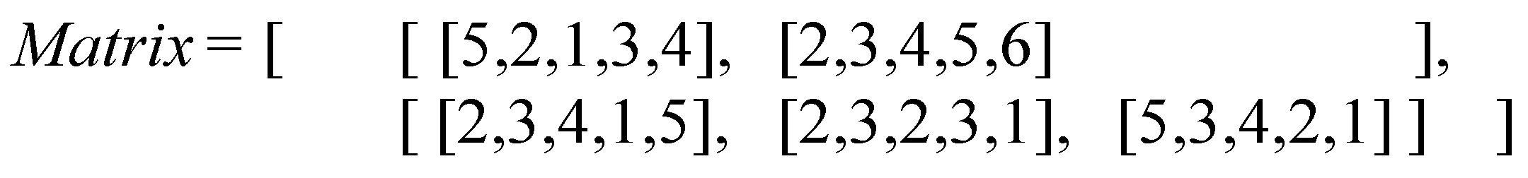
Figure 2 shows a Matrix containing two job processing times. According to the structure of the Matrix, it can be seen that job 1 requires two processes and job 2 requires 3 processes. And there are 5 available processing equipment. The processing time for each process on the 5 equipment is different. Therefore, to eliminate the randomness of processing time on a single machine, the pruning average method is used to measure the processing time required for each process. The metric for processing time of a process is defined as follows:
In Equation (11), tijk represents the processing time of process k of job i using equipment j, Mik represents the set of optional processing equipment for process k of job i, mik represents the amount of optional processing equipment for process k of job i, is the maximum processing time for process k of job i, and is the minimum processing time for process k of job i. Other metrics associated with processes can be calculated based on the processing time metric tik of the process, which includes the processing time of the next process (ti(h+1)), the total processing time of the remaining processes (), and the total processing time of the remaining processes except for the next process (). These metrics are represented as follows:
Process selection: the optimization goal is to minimize the maximum makespan. Therefore, the processing time of the process is the most important factor. The heuristic methods listed in Table 2-1 are all closely related to the processing time of the process. The selection result of the process for each decision can be calculated according to different rules based on the above metrics.
Equipment selection: during the equipment selection process, processing/transportation equipment is assigned to selected processes based on the the results of the process selection and equipment load balancing principle. The specific equipment selection process is shown in Algorithm 2. The input information of Algorithm 2 includes the process selection results (Olist) and the nested matrix of processing times for each process (Matrix), while the output information includes the equipment selection results (Mlist).
| Algorithm 2: Equipment selection process based on load balancing |
|
imput: Olist, Matrix output: Mlist 1: for i = 1 to m do 2: T m[i] ← 0 3: end for 4: for i = 1 to length (O list) do 5: H[i] ← Matrix[O list[i]] 6: for j = 1 to length(H) do 7: D[j] ← H[j] 8: for k = 1 to length(D) do 9: S [k] ← (T m[k]+D[k]) 10: end for 11: t min ← min(S) 12: p ← index(t min in S) 13: T m[p] ← t min 14: M list ← p 15: end for 16: end for 17: Return M list |
2.4. Policy Model
To improve exploration efficiency, the epsilon-greedy decreasing strategy is adopted. In the early iteration stage of this method, there is a higher probability of random selection to increase the diversity of the algorithm. As the number of iterations increases, the probability of random selection decreases while the probability of decision-making selection increases. There will be better convergence in the later stages of the iteration. The strategy can be expressed as:
In the Equation (14), ε is an initial parameter ranging from 0 to 1, n_step is a variable indicating the number of training times, and πbest(a) represents the optimal action selection result during the training period.
When the last training iteration is reached, the best action decision is output according to the policy πbest(a). At the beginning of the training, n_step is a very small number, and the probability of random action selection is high. As the training time increases, the value of n_step also increases. The probability of random action selection decreases, while the probability of decision action selection by the reinforcement learning model increases. With this strategy, more diverse solutions are explored in the early stage, and better and more stable solutions are obtained in the later stage.
2.5. Reward Fuction
The reward function is used to assess the level of impact of the current action on the state of the environment. In the problem proposed in this paper, when all process and equipment selections have been completed, the makespan can be used to evaluate the efficiency of the scheduling scheme. Therefore, a sparse reward approach is adopted where rewards for intermediate processes are set to zero. The intelligent agent is rewarded based on the quality of the scheduling result after all process and equipment selections are completed.
In most cases, the optimal value of the makespan for actual scheduling problems is unknown. Therefore, the time benchmark A in the current time progress of the state model in Section 2.2 is adopted. A normalization method for measuring rewards is designed, which improves the discrimination between results with different makespan. The time benchmark is a feasible solution obtained through genetic algorithms. If the makespan C obtained by the intelligent agent is less than , a negative reward is given. It indicates the punishment for intelligent agents. Conversely, if C is greater than or equal to , the intelligent agent receives a positive reward. The reward function is expressed as follows:
3. The Dynamic Scheduling Decision-Making Method Based on DRL
3.1. Algorithm Training Framework
In the DDQN algorithm, there are two deep neural networks with the same structure but different parameters, which are referred to as the main Q-network (parameters θ) and the target Q-network (parameters θ’). The main Q-network is used for agent decision-making, taking environmental states as inputs and outputting decision actions. The target Q-network is used to evaluate the quality of the main Q-network. The parameters θ of the main Q-network are periodically assigned to the parameters θ’ of the target Q-network. Therefore, the target Q-network has memories and experiences from the historical performance of the main Q-network, which can guide the decision-making of the main Q-network and reduce its overestimation. In the training process, the predicted Q-value obtained by the main Q-network is represented as follows:
Based on the Markov decision process and optimal strategy, the target Q-value obtained by the target Q-network can be expressed as Equation (17) (Van Hasselt et al., 2016).
Where γ is the discount factor that represents the decay of future rewards.
To prevent overestimation in the algorithm, the target Q-network corresponds its input behavior to the action that the main Q-network can obtain the maximum Q value, which is the most critical improvement of DDQN. Therefore, the Q-value update formula can be expressed as Equation (18), and the loss function can be expressed as Equation (19). In this paper, the gradient descent method is used to optimize the neural network parameters.
The memory replay method with priority experience is adopted for training to improve the training efficiency. The pseudo code of the DDQN-based training algorithm is shown in Algorithm 3.
| Algorithm 3: DDQN-based training algorithm |
| 1: Initialize the experience replay memory buffer D with capacity nmem 2: Initialize the main Q-network for action value function with random parameters θ 3: Initialize the target Q-network for action value function with parameters θ’ = θ 4: Obtain the initial state s1 and action a1 5: for t = 1 to Niter do 6: obtain st+1, rt 7: store (st, at, rt, st+1) to D 8: for t = 1 to T do 9: Use action selection policy to choose action at 10: Execute at in the environment state st, then obtain reward r and the next environment state st+1 11: store (st, at, rt, st+1) to D 12: If the number of experiences in D > a batch size nbatch, then 13: Select a batch size of (st, at, rt, st+1) from D based on priority experience. 14: Calculate , 15: Update θ using the gradient descent method according to and . 16: Reset θ’←θ every C steps. 17: Calculate the temporal difference error . 18: Update the priority of D based on. 19: end if 20: end for 21: end for |
The model training involves two processes: environment interaction process and main Q-network training processe. The training process is shown in Figure 3.
(1) Environment interaction process: the agent makes an action at based on the state st of the environment, then the environment outputs the next state st+1 and the reward rt. The data (st, at, st+1, rt) generated during each iteration is stored in the experience replay memory D. To improve the exploration ability of the algorithm, the policy introduced in Section 2.4 is adopted as the action decision-making policy of the agent. The amount of data stored in the experience replay memory buffer D is limited. When the buffer is full, the earliest stored data is removed and new data is stored.
(2) Main Q-network training processe: when the data stored in the experience replay memory buffer D is greater than a batch size (nbatch), a batch size data is selected from D according to the priority experience rule to train the main Q-network. The Q-value is predicted by the main Q-network, and the Q-value is evaluated by the target Q-network based on the Markov decision process. Finally, the parameters θ of the main Q-network are modified. To ensure that historical experience can be reflected in the evaluation process, the parameters θ’ are updated based on the parameters θ after each C-step cycle.
3.2. Dynamic Scheduling Decision-Making Method
Manufacturing resources in actual production mainly include processing equipment, transportation equipment (AGV), and jobs. Each type of manufacturing resource may consist of multiple individual entities. Tuples are defined to record the real-time status of each individual entity in each manufacturing resource. For example, if there are five processing equipment in the workshop, the processing equipment resource will consist of five processing equipment tuples.
Each equipment tuple contains multiple labels and content related to equipment status. The labels of the processing equipment tuples include “device number”, “assigned task”, “start node”, “end node”, and “end time”. The device number is the unique identifier of the equipment. The assigned tasks are in the form of a list of multiple [job number, process number], which records the information of the job and process to be processed on the equipment. The tuple packaging method is adopted to achieve lightweight expression of production information. The tuple information of these manufacturing resources reflects the production status in real-time, facilitating the statistical analysis of the real-time production environment status after disturbances.
The process of autonomous decision-making for dynamic scheduling problem is illustrated in Figure 4. According to the training process in Section 3.1, we train a model for intelligent agent to make scheduling decisions. When disturbances occur, the agent will make decisions and output the new scheduling plan in the form of a Gantt chart.
4. Event-Driven and Period-Driven Hybrid Dynamic Rescheduling
Rescheduling is used to solve scheduling problems with disturbances. In Section 3, a dynamic scheduling autonomous decision-making method based on DDQN is proposed to solve the problem of how to implement rescheduling. However, there are many disturbance factors in the production environment. If there are any disturbing factors and a rescheduling is performed, it will greatly undermine the stability of the scheduling system. Therefore, research on the rescheduling strategy and triggering mechanism is also crucial.
4.1. Rescheduling Triggering Mechanism
In practical manufacturing environments, some disturbances may cause the workshop to halt production at once, while others may result in the inability to execute the original production plan after a period of time. Therefore, an event-driven and period-driven hybrid dynamic rescheduling is used to handle such disturbances. The event-driven approach is used to address disturbances that have an immediate impact on the production. The period-driven approach is used to monitor the lag effects of disturbances and to address them in a timely manner at periodic intervals to prevent impacts on subsequent production. This approach improves both the responsiveness and stability of dynamic scheduling.
In the Figure 5, it shows the implementation process of the dynamic rescheduling trigger strategy combining period-driven and period-driven methods. Based on the early-stage static scheduling results, a dynamic scheduling process is implemented with a series of preparatory steps at the initial stage. These steps can be divided into two parts:
Step 1: GA is used to compute the static scheduling plan for the unfinished jobs in order to obtain a complete scheduling plan and Gantt chart.
Step 2: Based on the scheduling plan obtained from Step 1, the periodic trigger points are determined by dividing the total number of manufacturing processes in the training agent. Since multiple devices work in parallel, it is difficult to determine the periodic trigger points. Therefore, the completion time during training is used as the basis for determining the periodic trigger points.
After completing these two steps, the scheduling plan is executed sequentially according to periodic windows. During the execution process of the scheduling plan, it is judged at each periodic trigger point whether the rescheduling needs to be triggered. If there is no disturbance event, the production process will follow the initial scheduling plan and complete each window task in sequence. If a disturbance event occurs, it is judged whether the disturbance event needs to trigger the rescheduling immediately. If the disturbance event has no effect on the current window task, the event-driven rescheduling does not need to be triggered at this time. Instead, the impact of the disturbance event on the processing-related resource changes will be adjusted in the next periodic trigger point, followed by the re-determination of the scheduling plan. If the disturbance event affects the current window task of the scheduling plan, the event-driven rescheduling needs to be triggered immediately.
When a disturbance is triggered, the job that has already been completed is not affected. Whether the job being processed is affected by the disturbance needs to be discussed in detail. When the disturbance does not affect the job being processed, the job continues to be processed according to the original plan. If the disturbance affects the job being processed, the process is stopped and joins the rescheduling with the process steps of the unprocessed jobs.
4.2. Dynamic Rescheduling Implementation Method
A dynamic scheduling implementation method with judgment based on DDQN is proposed. In the initial stage, the current scheduling plan is calculated based on the optimization algorithm, and more time can be spent in this process to calculate better solutions. Production is carried out according to the established scheduling plan, and disturbance events are monitored in real-time. If a disturbance event is detected, the algorithm will make a series of judgments to determine whether and when to reschedule. This approach minimizes the number of reschedulings and improves the stability of dynamic scheduling. The following are explanations for the four judgment conditions shown in Figure 6.
① Real-time disturbance judgement: it is the first judgment condition for the scheduling system after receiving a disturbance and it will determine whether the disturbance needs to be handled immediately. It will be determined in this stage whether the disturbance event will affect the current production plan. In general, equipment failures and time delays will directly affect the original production plan, so event-driven rescheduling will be triggered. However, disturbance caused by order changes are usually additional orders, and these additional orders are generally arranged for follow-up production planning in the next cycle node. In addition, there are other disturbances that do not need to be handled immediately, such as when a faulty equipment is no longer involved in the tasks being executed in the current time window, the disturbance will be handled in the next cycle node.
② Periodic node arrival judgement: it used for determining if the progress has reached the trigger node of the cycle. If the disturbance event does not affect the execution of the current window plan and the current progress has not yet reached the pre-set cycle node, the original scheduling plan will be executed. When the cycle node is reached, the production status and production tasks are analyzed and processed.
③ Periodic node handling judgment: when the scheduling reaches a periodic node, it is used to determine whether there are any non-real-time disturbances from the previous cycle that need to be processed. If the previous execution period did not change the production state, the original production plan is executed. If there was a non-instantaneous disturbance in the previous period that will change the current production resource state, it triggers a periodic-driven rescheduling.
④ Task completion judgment: it used to monitor whether the scheduling task is completed. If the scheduling task is not completed, it will be carried out according to the original plan. If the scheduling task is completed, the program will be terminated.
When disturbances occur, a series of judgments will be made to determine when to reschedule. The specific process is shown in Figure 4-2. Once rescheduling is required, the trigger condition for rescheduling is input, and then the scheduling plan for the executing window and the remaining tasks are output.
In Figure 7, it shows the implementation rescheduling process under equipment failure. When equipment failure disturbances occur, current environmental state information is got. The agent quickly makes decisions on task scheduling for the upcoming execution window, and divides the cycle nodes for remaining processes. The remaining tasks after the upcoming execution windows waiting for process have low real-time requirements, so evolutionary algorithms can be used to obtain an excellent solution.
5. Data Experimentation and Analysis
5.1. Introduction to Experimental Data
This paper mainly studies the dynamic scheduling problem of FJSP. Therefore, Kacem dataset is select as the basic data for experimental research. There are four different data sizes in the dataset, namely Kacem 4×5, Kacem 8×8, Kacem 10×10, and Kacem 15×10. Different datasets contain different processing information, for example, Kacem 4×5 indicates that there are four types of jobs and five machines in the production environment. In Table 2, it is shown the specific parameters of the Kacem 4×5 dataset. The transportation time between two nodes is set as a random number between 0.5 and 1.5 according to the processing time value range of Kacem dataset. Table 3 shows the transportation time for Kacem 4×5. Similarly, the transportation time of the Kacem 8×8, Kacem 10×10, and Kacem 15×10 dataset is generated using above method, which is used for data experiments.
5.2. Model Training for Different Problems
The algorithm randomly selects job numbers from the Kacem 4×5, Kacem 8×8, Kacem 10×10, and Kacem 15×10 datasets. Two orders with a total of 20 jobs are generated for each dataset, and the first order is used for the initial training of the agent. Based on the trained main Q-network model parameters for order one, the second order is used for the continued training of the main Q-network using the method of breakpoint continuation training. Figure 8, Figure 9, Figure 10 and Figure 11 respectively show the training process for the two orders in the four different problems.
The results show indicate that in the first training process of all datasets, the main Q-network focuses on exploration in the early stages and gradually converges, and the rewards obtained gradually stabilize in the later stage. Due to the foundation of the first training, the second training can quickly maintain stable and good output. The main Q-network can make good decisions and obtain good rewards from the start, and maintain a relatively stable state in subsequent training. In the two training processes, the production environment and product type are consistent, but the order quantity is different. Therefore, it can be confirmed that the trained main Q-network has the ability to make different decisions for different orders.
Table 4 and Table 5 show the computational results for the proposed method and other methods for the 10 orders in Kacem 4×5 dataset. Table 6 and Table 7 show the computational results for different methods for the 10 orders in Kacem 8×8 dataset. Table 8 and Table 9 show the computational results for different methods for the 10 orders in Kacem 10×10 dataset. Table 10 and Table 11 show the computational results for different methods for the 10 orders in Kacem 15×10 dataset. Numbers 1 to 10 represent different order numbers. Eight heuristic rule methods (in Table 1), genetic algorithm, and trained model by the proposed method were compared. The performance of the algorithms was evaluated using the makespan and decision calculation time.
The following conclusions can be drawn from the comparative experiments of data from orders of different sizes. Evolutionary optimization algorithms represented by genetic algorithms can obtain good feasible solutions in most problems, but require more computational time. Although heuristic rules have fast decision-making speeds, the stability of the resulting solutions is insufficient. The trained DDQN decision model is able to make decisions quickly while obtaining good solution results in most problems.
5.3. Dynamic Scheduling Case Study
A 20-job order was randomly generated based on the Kacem 4×5 dataset. The order was scheduled using genetic algorithm to obtain the initial scheduling plan as shown in Figure 12 and Figure 13. These two figures represent the scheduling plan of jobs and equipment, respectively. In the figures, the blue block represents no-load transportation process, the green block represents load transportation process, and the white block represents processing process. For the job scheduling plan in Figure 12, the three numbers in parentheses respectively represent the job process, the processing equipment number, and the transportation equipment number. For the equipment scheduling plan in Figure 13, the numbers in parentheses for processing equipment respectively represent the job number and the job process number, and the numbers for transportation equipment represent the job number. The final blue vertical line represents the makespan on the scheduling plan, which is 60.46.
Figure 12 and Figure 13 show the scheduling plan obtained using genetic algorithm, which serves as the initial scheduling plan. Based on this case, dynamic scheduling verification experiments are conducted under the influence of disturbance factors. The disturbance factors include three typical sources of uncertainty: equipment failure, processing times lag, and order changes.
5.3.1. Equipment Failure Disturbance Case
Once a processing equipment is failure, it is necessary to allocate the tasks from the faulty equipment to other similar equipment to reduce the impact of equipment failures on production schedules.
Equipment failure is assumed to occur in processing equipment M1 at 25 seconds, as shown in Figure 14. At 25 seconds, the jobs being processed are (5,3) on M1, (1,1) on M3, and (12,3) on M5. The jobs currently being handled by the transportation equipment are (3,1) on T1, and (9,1) on T2. These processes are in progress when the disturbance is triggered.
The job 5 being processed by equipment M1 is non-conforming due to a failure of equipment M1. Therefore, job 5 must to be reprocessed. In the subsequent rescheduling, job 5 will be treated as a new job and processed from the raw material stage. The remaining equipment in operation will continue to complete the current processing step after the disturbance occurs. Therefore, the allowed rescheduling start time for this equipment is the moment when the current task is completed. If the equipment is not in operation when the disturbance occurs, then the allowed rescheduling start time for this equipment is rescheduled zero time.
Manufacturing resource information is used as a constraint for rescheduling, and these constraints are considered when making decisions in the main Q-network. Figure 15 shows the rescheduling results obtained from the main Q-network. It spends 2.44 seconds from the trigger of the disturbance to make the decision. The equipment failure disturbance occurred at 25 seconds. The original scheduling plan was executed before 25 seconds, and the rescheduling plan was executed after 25 seconds. Job 5 on faulty equipment M1 has been reprocessed in the rescheduling plan, as shown in Figure 15.
In addition, for the transportation process, the transportation equipment will continue to complete the current transportation task when a disturbance occurs. As shown in Figure 14., at the time of disturbance, the process (3, 1) is being transported to M4 by T1. The rescheduling plan shown in Figure 15 still arranges the process (3, 1) to transport to M4 by T1. However, for T2, the process (9, 1) is being transported to M1 at the time of disturbance. Process (9, 1) was affected by faulty equipment M1 and the assigned processing equipment was changed. Therefore, in the rescheduling plan shown in Figure 15, process (9, 1) was rescheduled to be transported to M3.
5.3.2. Processing Time Lag Disturbance Case
Based on the original production plan (in Figure 13), processing time lag is assumed to occur in processing time of process (17,1) on machine M3. In the original plan, process (17,1) should end at 20.84 seconds. However, the disturbance is expected to cause a delay of 15 seconds on top of the original processing time. Therefore, the triggering time of the disturbance is at 20.84 seconds. This phenomenon will affect subsequent operations and trigger event-driven rescheduling.
Figure 16 shows the rescheduling triggered by a processing time lag event. The triggering node is set to the normal completion time of process (17,1), which is 20.84 seconds. Other operations that are being processed at this time node include (19,2) and (20,1), which will continue to be completed. The delayed operation (17,1) will continue to complete the task according to the expected delay time of 15 seconds. The allowed start time node for subsequent operation (17,2) is set to 35.84 seconds, and the allowed start time for M3 is also set to 35.84 seconds.
The result of rescheduling triggered by a processing delay disturbance is shown in Figure 17. The triggering node is at 20.84 seconds. The original scheduling plan was executed before 20.84 seconds. After 20.84 seconds, the scheduling result determined by the trained master Q-network is executed. The decision-making time for this process is 2.5 seconds.
5.3.3. Order Change Disturbance Case
Since order change disturbance generally does not directly affect the current task being performed, this type of disturbance event will be processed at the cycle node. It will reduce rescheduling times and improve the stability of dynamic scheduling.
Based on the Kacem 4x5 dataset, orders for 40 jobs were randomly generated, and a genetic algorithm was used to calculate the production schedule for the orders. The initial scheduling plan obtained is shown in Figure 18. The cycle time was set to 60 seconds. Every 60 seconds, the system will check the current manufacturing resource information. If the manufacturing resource information has not changed, the cycle-driven rescheduling will not be triggered, and the production will continue according to the original plan. To facilitate the display of job information, the job number is only displayed on the processing equipment.
The result of rescheduling triggered by an order disturbance is shown in Figure 19. The order change occurred between 0-60 seconds, so the rescheduling was triggered at the first dynamic scheduling cycle node after the order change disturbance, which was at 60 seconds. At this moment, the newly added orders are included in the calculation range of the algorithm, and the tasks that need to be completed by the orders are reorganized. The original scheduling plan was executed before 60 seconds. After 60 seconds, the scheduling plan determined by the main Q-network was executed. The decision-making time was 12.45 seconds due to the large amount of calculation, which resulted in a corresponding increase in response time. However, it can still be considered that the algorithm quickly provided a scheduling solution.
6. Conclusion
In this paper, dynamic scheduling based on reinforcement learning under uncertain disturbance factors is studied. The real-time status composition of production workshop scheduling is analyzed, and a DRL environment model of FJSP is established. A high-quality rescheduling decision-making method and a highly responsive rescheduling trigger mechanism are proposed. The effectiveness of this algorithm is verified through data experiments and actual disturbances. The solution for dynamic scheduling under disturbance factors with high responsiveness and quick feedback is studied from multiple aspects, including DRL environment modeling, DRL algorithm design and training, rescheduling trigger mechanism, and data experiment verification. The conclusions of this paper are as follows:
(1) A real-time DRL production environment model consisting of production status, action, policy, and reward function is established. The status consists of the current number of completed processes, current time progress, processing equipment idle status, and transportation equipment idle status. The scheduling decision is used as the action model, and the scheduling result is used as the reward function.
(2) A dynamic scheduling decision-making method based on DRL is studied, and a training algorithm combining GA and DDQN is proposed. Based on GA, the reward benchmark is established in the initial training stage. The model is trained based on DDQN, and the autonomous scheduling decision-making after disturbance is realized.
(3) An event-driven and period-driven hybrid dynamic rescheduling is proposed based on the trained DRL decision model. The cycle node is based on the number of jobs in the DRL training model. This triggering mechanism effectively controls the rescheduling calculation times and improves the stability of the dynamic scheduling system.
The data experiment results show that the trained DRL dynamic scheduling decision-making model can provide timely feedback on the adjusted scheduling arrangements for different-scale order problems. In particular, compared with metaheuristic algorithms, the decision-making time is improved from minutes to seconds, which is a significant improvement. The decision results of the DRL dynamic scheduling model can provide better solutions for most problems. Dynamic scheduling decision-making process application verification is carried out based on disturbance factors such as equipment failure, processing time lag, and order changes. The proposed dynamic scheduling decision-making method and rescheduling trigger strategy can realize high responsiveness, quick feedback, high quality, and high stability of autonomous dynamic scheduling decision-making.
Acknowledgements
The authors are grateful for financial support from the the National Natural Science Foundation of China (No. 52405527).
References
- Adibi, M.A., Shahrabi, J., 2014. A clustering-based modified variable neighborhood search algorithm for a dynamic job shop scheduling problem. The International Journal of Advanced Manufacturing Technology 70, 1955-1961. [CrossRef]
- Adibi, M.A., Zandieh, M., Amiri, M., 2010. Multi-objective scheduling of dynamic job shop using variable neighborhood search. Expert Systems with Applications 37, 282-287. [CrossRef]
- Baykasoğlu, A., Madenoğlu, F.S., Hamzadayı, A., 2020. Greedy randomized adaptive search for dynamic flexible job-shop scheduling. Journal of Manufacturing Systems 56, 425-451. [CrossRef]
- Ding, G.Z., Guo, S.Y., Wu, X.H., 2022. Dynamic Scheduling Optimization of Production Workshops Based on Digital Twin. Applied Sciences-Basel 12, 16. [CrossRef]
- Ghaleb, M., Taghipour, S., 2023. Dynamic shop-floor scheduling using real-time information: A case study from the thermoplastic industry. Computers & Operations Research 152. [CrossRef]
- Ghaleb, M., Taghipour, S., Zolfagharinia, H., 2021. Real-time integrated production-scheduling and maintenance-planning in a flexible job shop with machine deterioration and condition-based maintenance. Journal of Manufacturing Systems 61, 423-449. [CrossRef]
- Hamzadayi, A., Yildiz, G., 2016. Event driven strategy based complete rescheduling approaches for dynamic m identical parallel machines scheduling problem with a common server. Computers & Industrial Engineering 91, 66-84. [CrossRef]
- Han, B., Yang, J.-J., 2020. Research on Adaptive Job Shop Scheduling Problems Based on Dueling Double DQN. IEEE Access 8, 186474-186495. [CrossRef]
- He, X.M., Dong, S.H., Zhao, N., 2020. Research on rush order insertion rescheduling problem under hybrid flow shop based on NSGA-III. International Journal of Production Research 58, 1161-1177. [CrossRef]
- Hu, H., Jia, X., He, Q., Fu, S., Liu, K., 2020. Deep reinforcement learning based AGVs real-time scheduling with mixed rule for flexible shop floor in industry 4.0. Computers & Industrial Engineering 149, 106749. [CrossRef]
- Kamali, S.R., Banirostam, T., Motameni, H., Teshnehlab, M., 2023. An immune-based multi-agent system for flexible job shop scheduling problem in dynamic and multi-objective environments. Engineering Applications of Artificial Intelligence 123, 106317. [CrossRef]
- Khodke, P., Bhongade, A., 2013. Real-time scheduling in manufacturing system with machining and assembly operations: A state of art. International Journal of Production Research 51, 4966-4978. [CrossRef]
- Kouider, A., Bouzouia, B., 2012. Multi-agent job shop scheduling system based on co-operative approach of idle time minimisation. International Journal of Production Research 50, 409-424. [CrossRef]
- Kundakcı, N., Kulak, O., 2016. Hybrid genetic algorithms for minimizing makespan in dynamic job shop scheduling problem. Computers & Industrial Engineering 96, 31-51. [CrossRef]
- Laili, Y., Peng, C., Chen, Z., Ye, F., Zhang, L., 2022. Concurrent local search for process planning and scheduling in the industrial Internet-of-Things environment. Journal of Industrial Information Integration 28, 100364. [CrossRef]
- Li, Y., Gu, W., Yuan, M., Tang, Y., 2022. Real-time data-driven dynamic scheduling for flexible job shop with insufficient transportation resources using hybrid deep Q network. Robotics and Computer-Integrated Manufacturing 74, 102283. [CrossRef]
- Lu, C., Gao, L., Li, X., Xiao, S., 2017. A hybrid multi-objective grey wolf optimizer for dynamic scheduling in a real-world welding industry. Engineering Applications of Artificial Intelligence 57, 61-79. [CrossRef]
- Lu, S., Pei, J., Liu, X., Pardalos, P.M., 2021a. A hybrid DBH-VNS for high-end equipment production scheduling with machine failures and preventive maintenance activities. Journal of Computational and Applied Mathematics 384, 113195. [CrossRef]
- Lu, S.J., Pei, J., Liu, X.B., Pardalos, P.M., 2021b. A hybrid DBH-VNS for high-end equipment production scheduling with machine failures and preventive maintenance activities. Journal of Computational and Applied Mathematics 384, 16. [CrossRef]
- Luo, S., 2020. Dynamic scheduling for flexible job shop with new job insertions by deep reinforcement learning. Applied Soft Computing 91, 106208. [CrossRef]
- Mnih, V., Kavukcuoglu, K., Silver, D., Rusu, A.A., Veness, J., Bellemare, M.G., Graves, A., Riedmiller, M., Fidjeland, A.K., Ostrovski, G., Petersen, S., Beattie, C., Sadik, A., Antonoglou, I., King, H., Kumaran, D., Wierstra, D., Legg, S., Hassabis, D., 2015. Human-level control through deep reinforcement learning. Nature 518, 529-533. [CrossRef]
- Ning, T., Huang, M., Liang, X., Jin, H., 2016. A novel dynamic scheduling strategy for solving flexible job-shop problems. Journal of Ambient Intelligence and Humanized Computing 7, 721-729. [CrossRef]
- Nouiri, M., Bekrar, A., Trentesaux, D., 2018. Towards Energy Efficient Scheduling and Rescheduling for Dynamic Flexible Job Shop Problem. IFAC-PapersOnLine 51, 1275-1280. [CrossRef]
- Park, J., Mei, Y., Nguyen, S., Chen, G., Zhang, M., 2018. An investigation of ensemble combination schemes for genetic programming based hyper-heuristic approaches to dynamic job shop scheduling. Applied Soft Computing 63, 72-86. [CrossRef]
- Shi, D., Fan, W., Xiao, Y., Lin, T., Xing, C., 2020a. Intelligent scheduling of discrete automated production line via deep reinforcement learning. International Journal of Production Research 58, 3362-3380. [CrossRef]
- Shi, D., Zhang, B., Li, Y., 2020b. A Multi-Objective Flexible Job-Shop Scheduling Model Based on Fuzzy Theory and Immune Genetic Algorithm. International Journal of Simulation Modelling 19, 123-133. [CrossRef]
- Shiue, Y.-R., Lee, K.-C., Su, C.-T., 2018. Real-time scheduling for a smart factory using a reinforcement learning approach. Computers & Industrial Engineering 125, 604-614. [CrossRef]
- Stevenson, Z., Fukasawa, R., Ricardez-Sandoval, L., 2020. Evaluating periodic rescheduling policies using a rolling horizon framework in an industrial-scale multipurpose plant. Journal of Scheduling 23, 397-410. [CrossRef]
- Van Hasselt, H., Guez, A., Silver, D., 2016. Deep Reinforcement Learning with Double Q-Learning. Proceedings of the AAAI Conference on Artificial Intelligence 30. [CrossRef]
- Wang, C.N., Hsu, H.P., Fu, H.P., Phan, N.K.P., Nguyen, V.T., 2022. Scheduling Flexible Flow Shop in Labeling Companies to Minimize the Makespan. Computer Systems Science and Engineering 40, 17-36. [CrossRef]
- Wang, L., Hu, X., Wang, Y., Xu, S., Ma, S., Yang, K., Liu, Z., Wang, W., 2021. Dynamic job-shop scheduling in smart manufacturing using deep reinforcement learning. Computer Networks 190, 107969. [CrossRef]
- Yan, J., Liu, Z., Zhang, C., Zhang, T., Zhang, Y., Yang, C., 2021. Research on flexible job shop scheduling under finite transportation conditions for digital twin workshop. Robotics and Computer-Integrated Manufacturing 72, 102198. [CrossRef]
- Yu, S.-p., Pan, Q.-k., 2012. A Rescheduling Method for Operation Time Delay Disturbance in Steelmaking and Continuous Casting Production Process. Journal of Iron and Steel Research International 19, 33-41. [CrossRef]
Figure 1.
Scheduling implementation process of reinforcement learning.
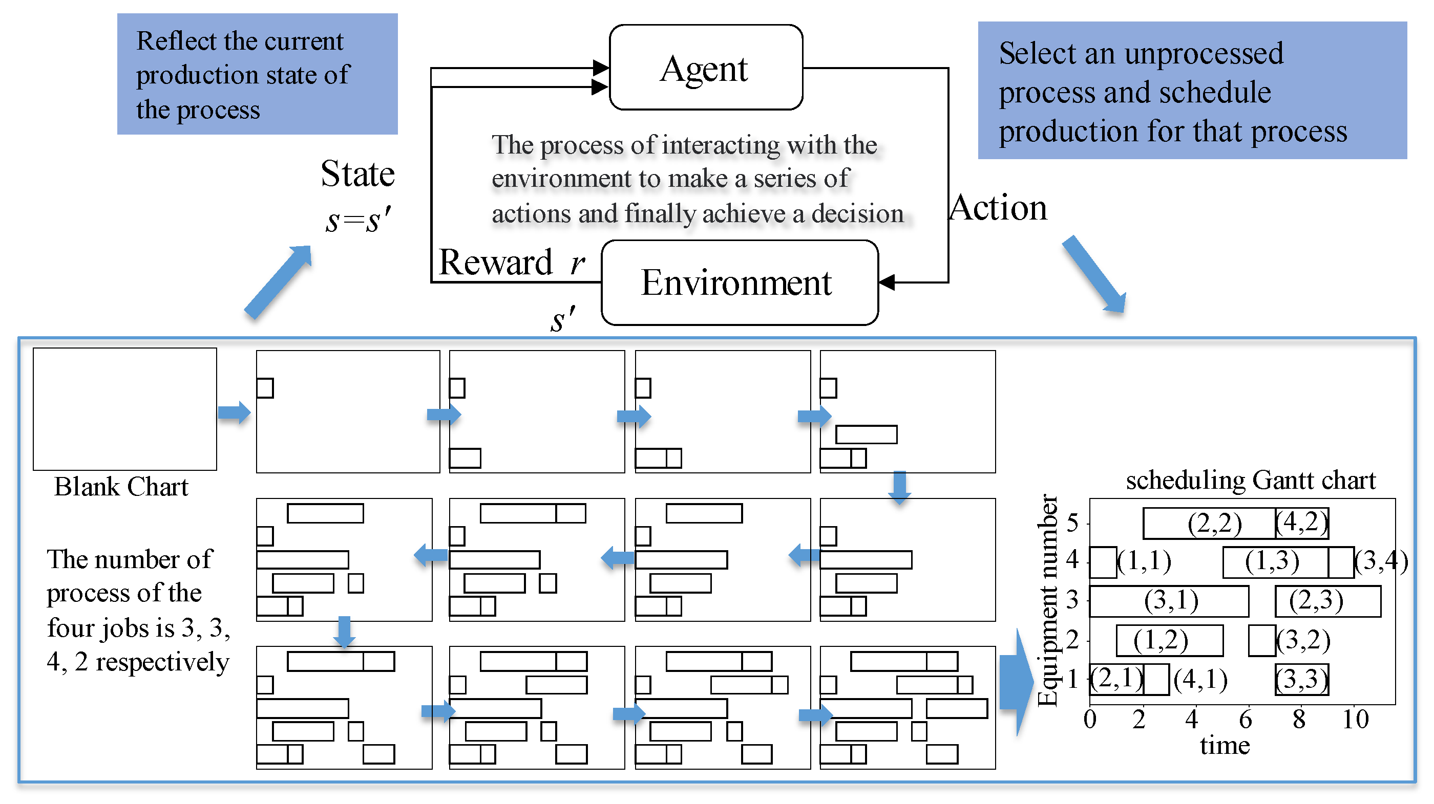
Figure 2.
Time composition of an operation.
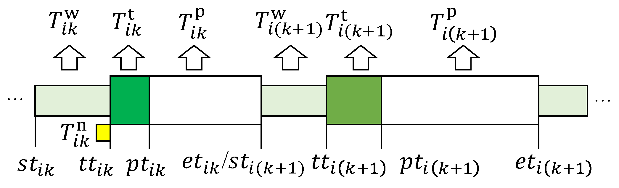
Figure 3.
Scheduling decision training process based on DDQN.
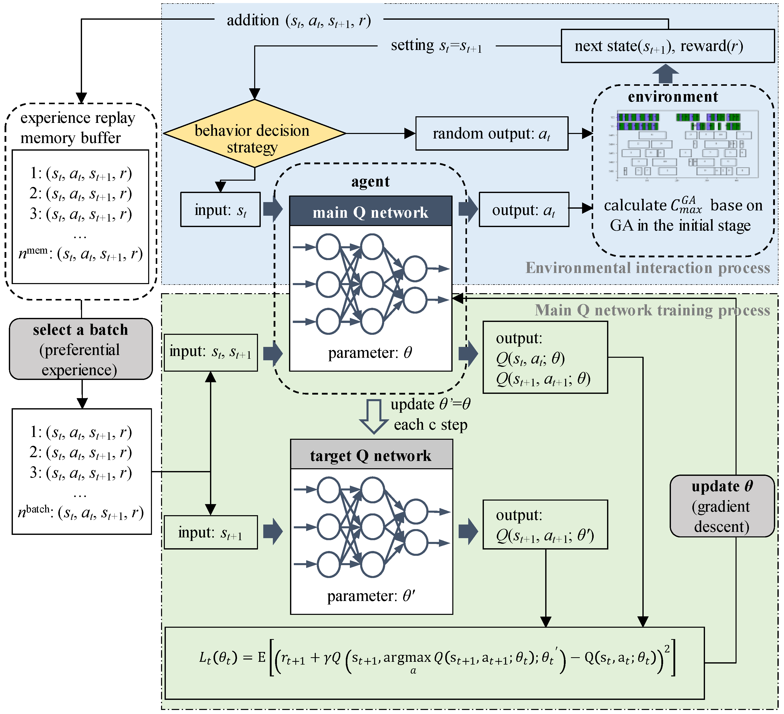
Figure 4.
Decision process of dynamic scheduling problem.
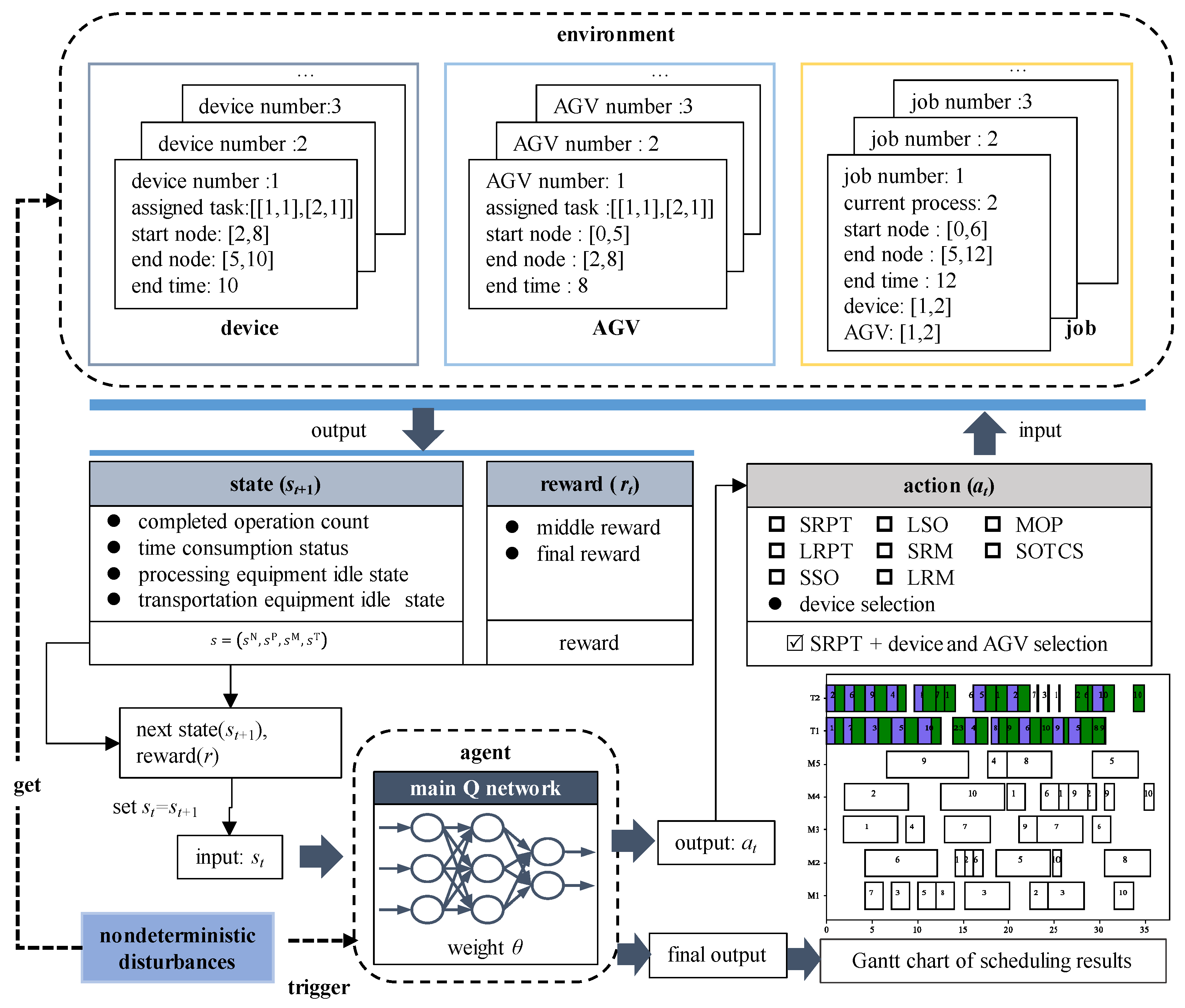
Figure 5.
Dynamic rescheduling trigger mechanism.
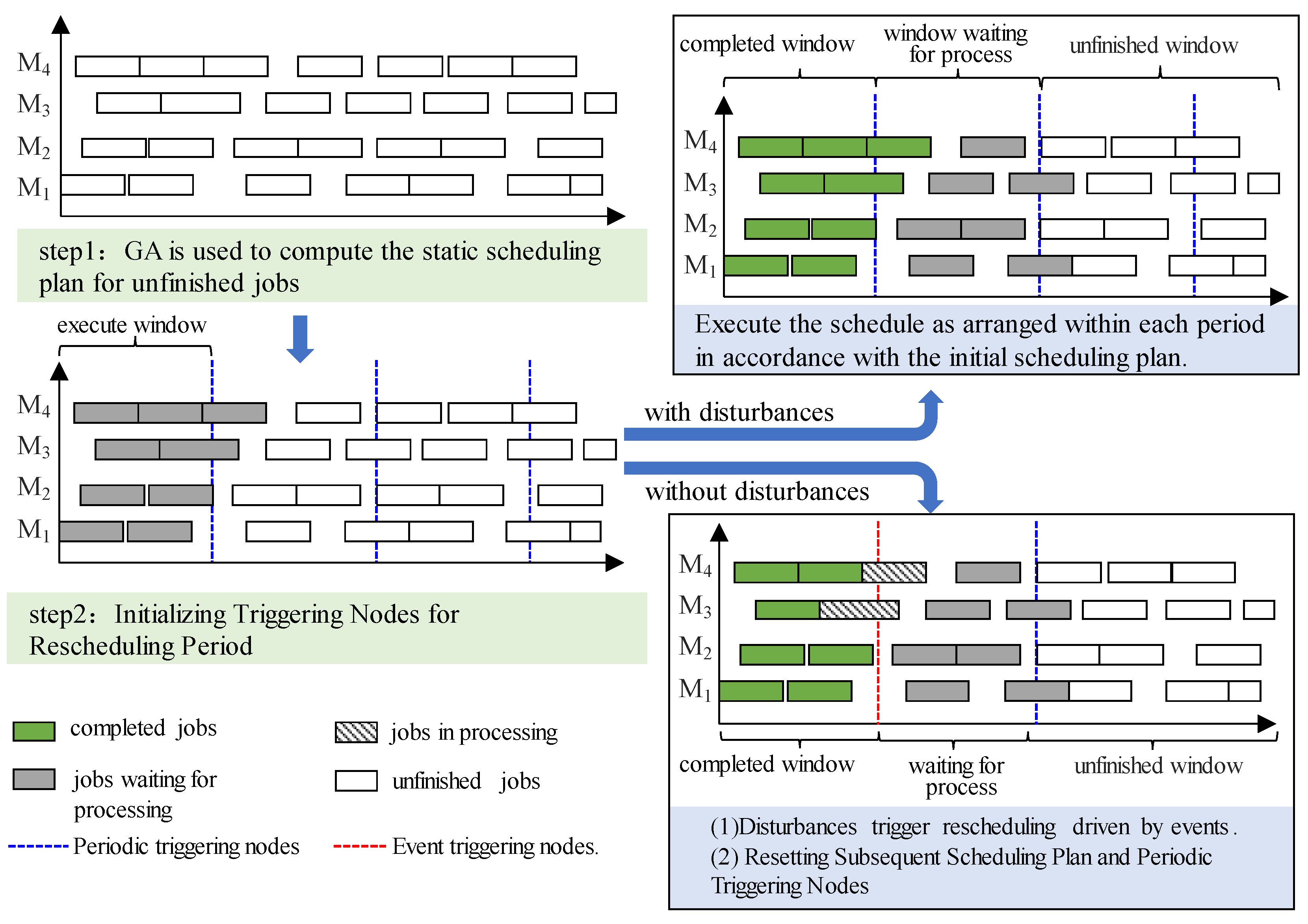
Figure 6.
Dynamic scheduling flowchart.
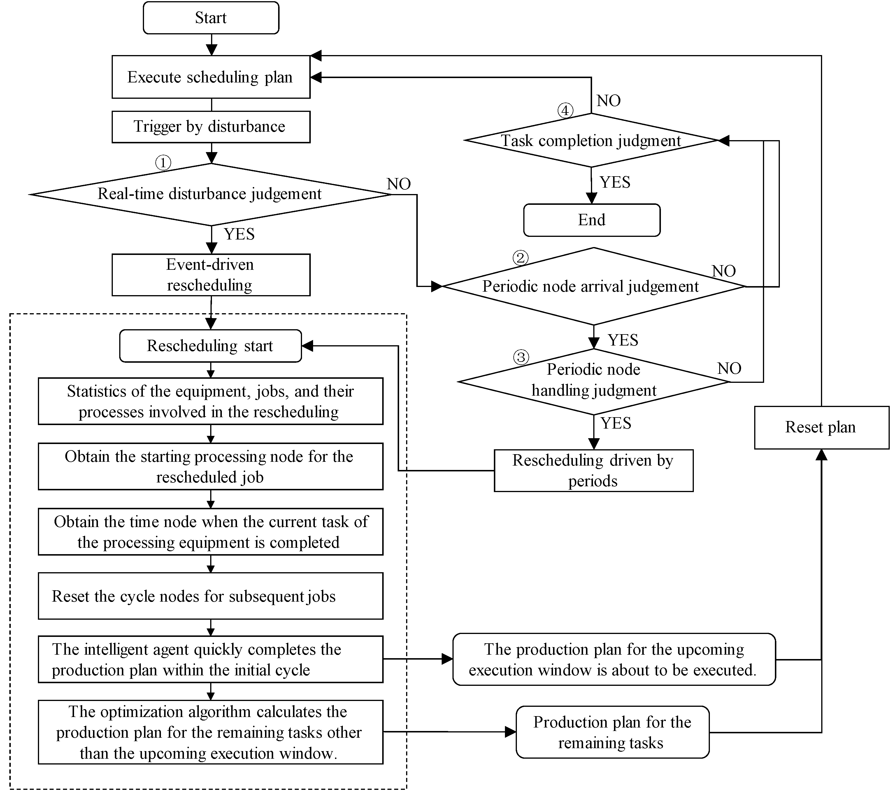
Figure 7.
Rescheduling implementation process.
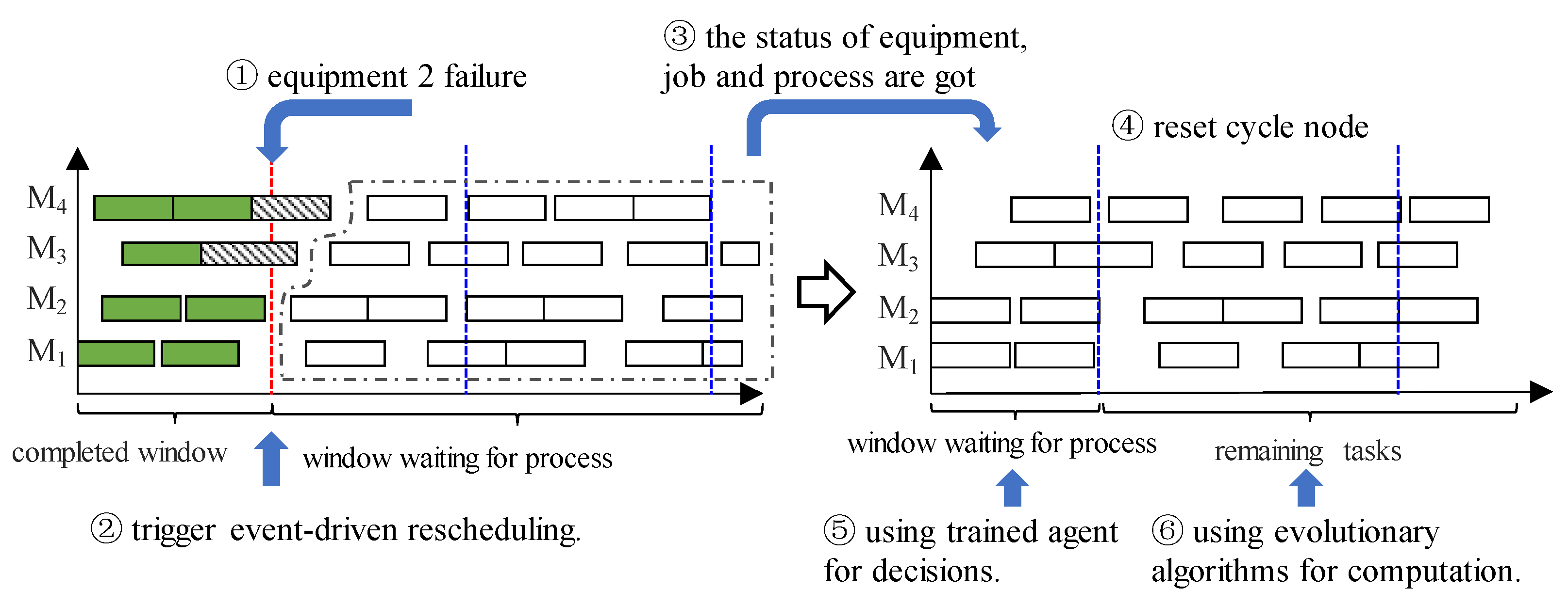
Figure 8.
Breakpoint continuation process of two orders based on Kacem 4×5.
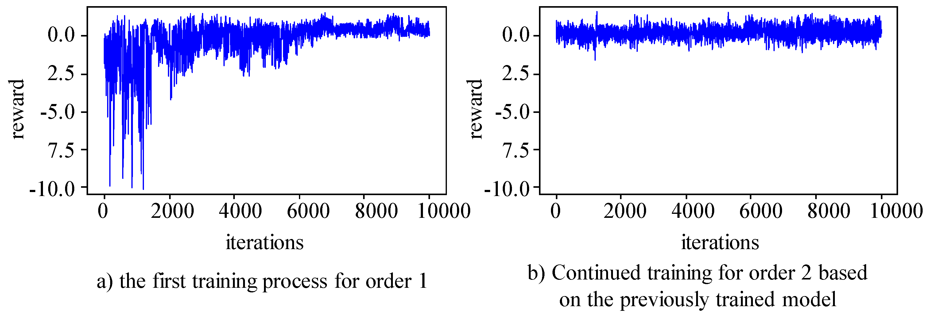
Figure 9.
Breakpoint continuation process of two orders based on Kacem 8×8.
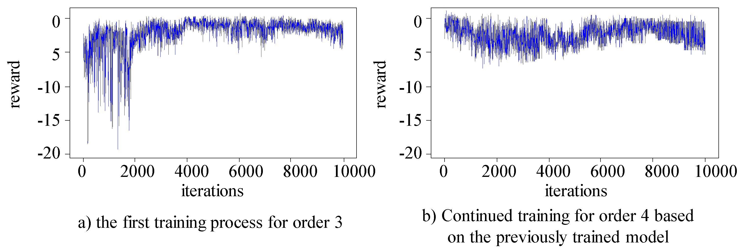
Figure 10.
Breakpoint continuation process of two orders based on Kacem 10×10.
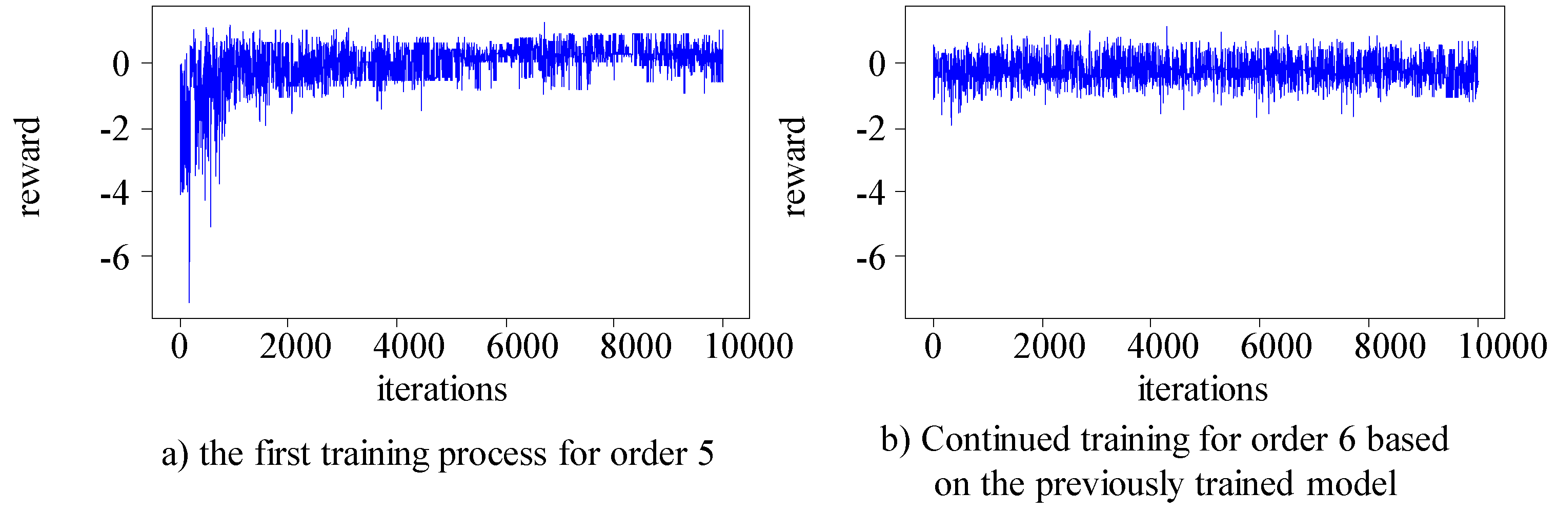
Figure 11.
Breakpoint continuation process of two orders based on Kacem 15×10.
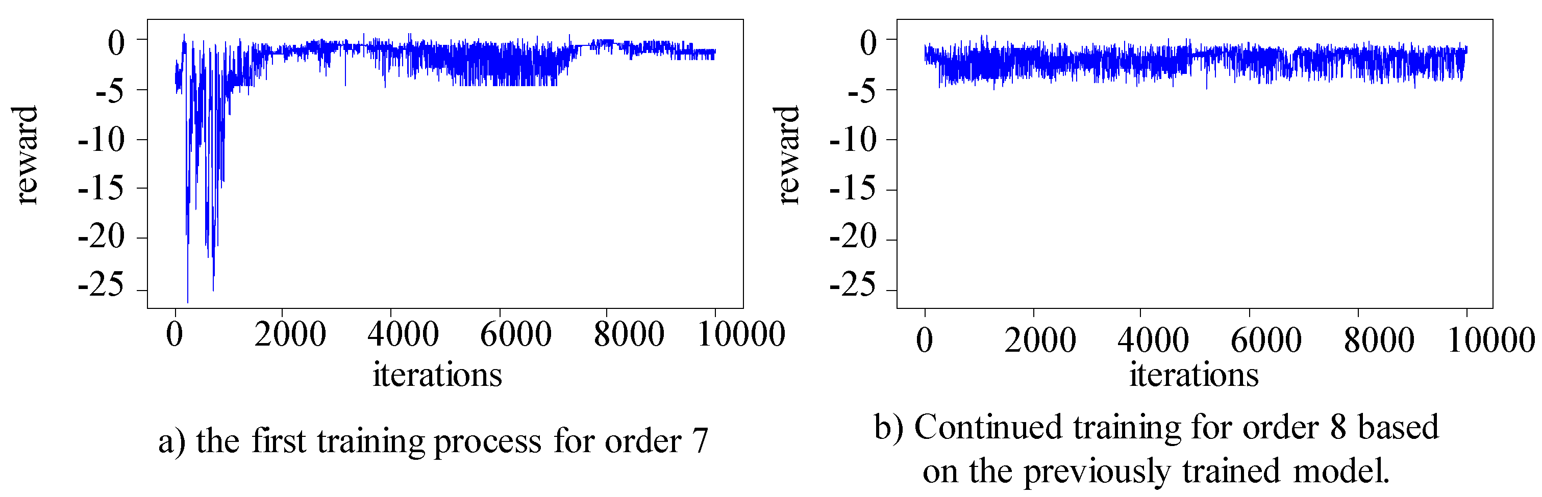
Figure 12.
Gantt chart of jobs scheduling plan.
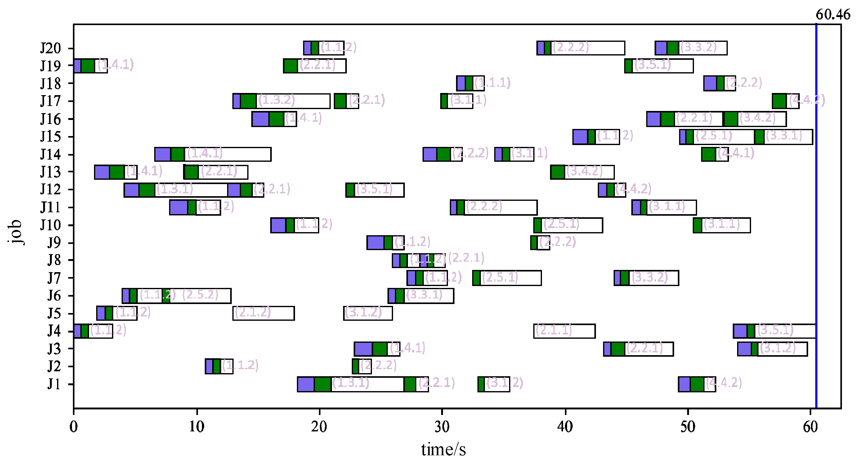
Figure 13.
Gantt chart of machines scheduling plan.
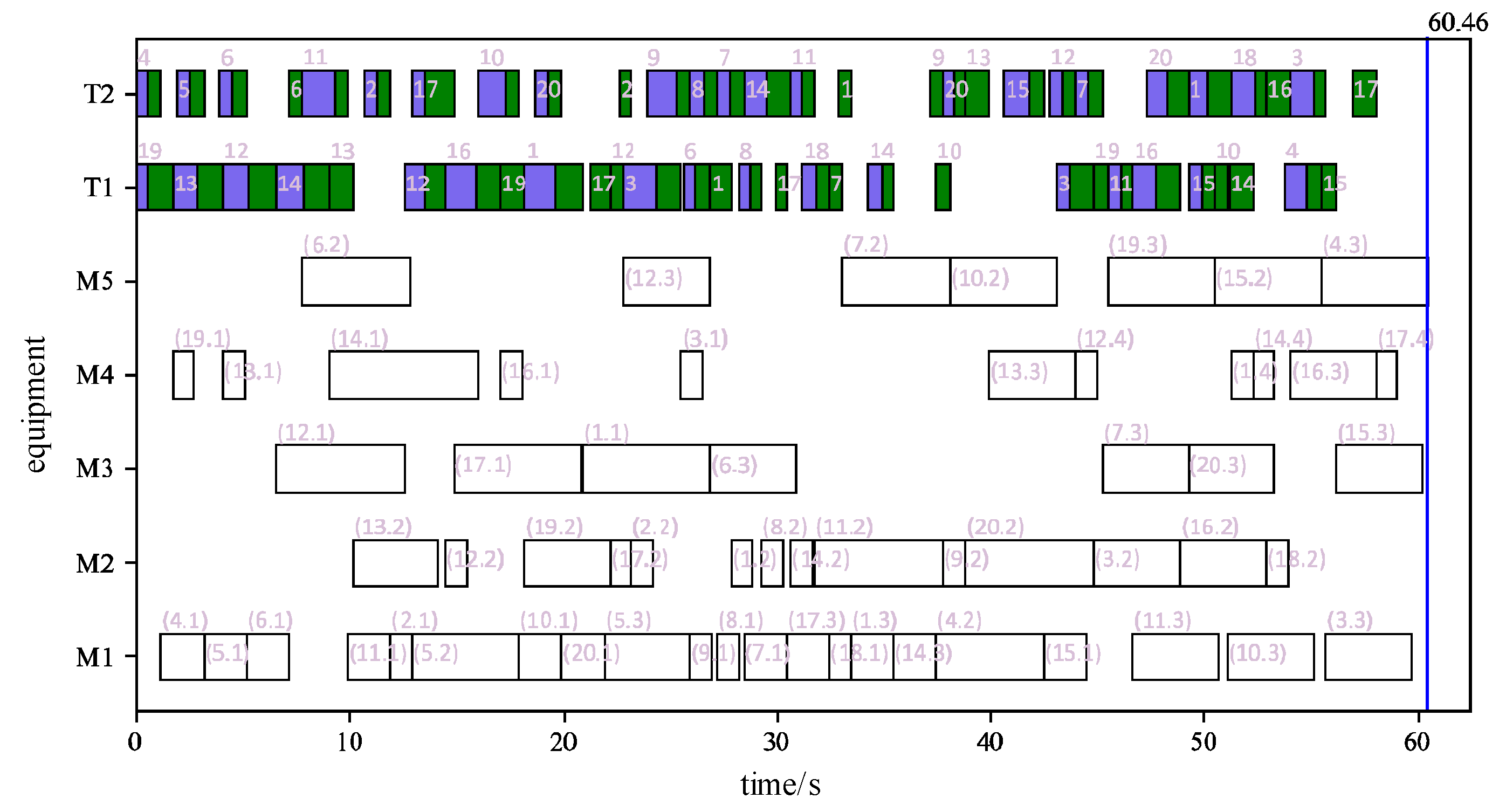
Figure 14.
Equipment failure event triggers rescheduling.
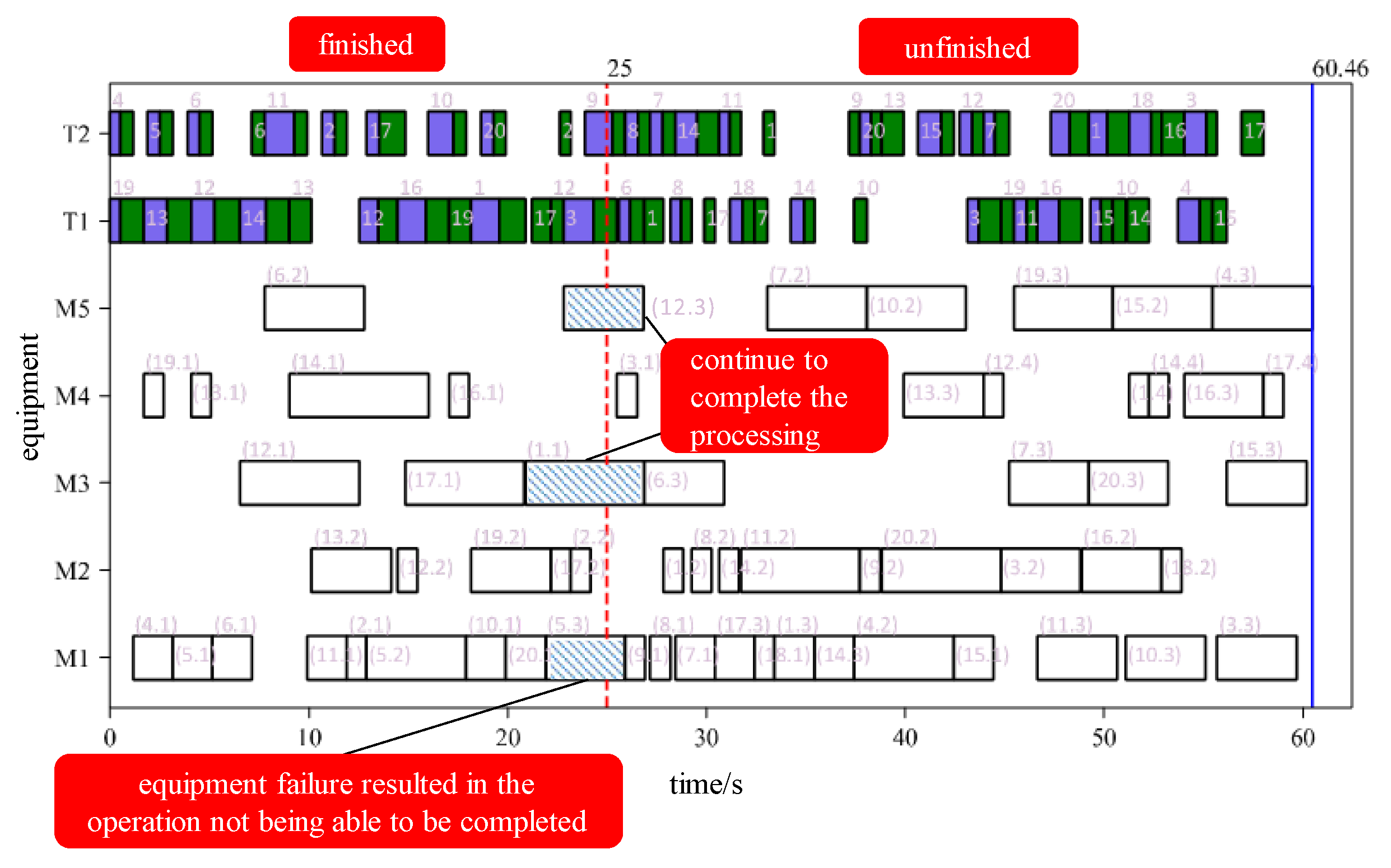
Figure 15.
Rescheduling results after triggering of equipment fault disturbance.
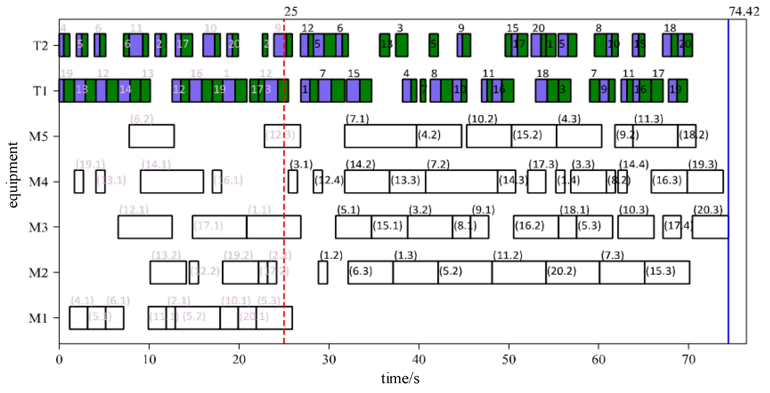
Figure 16.
Processing time lag event triggers rescheduling.
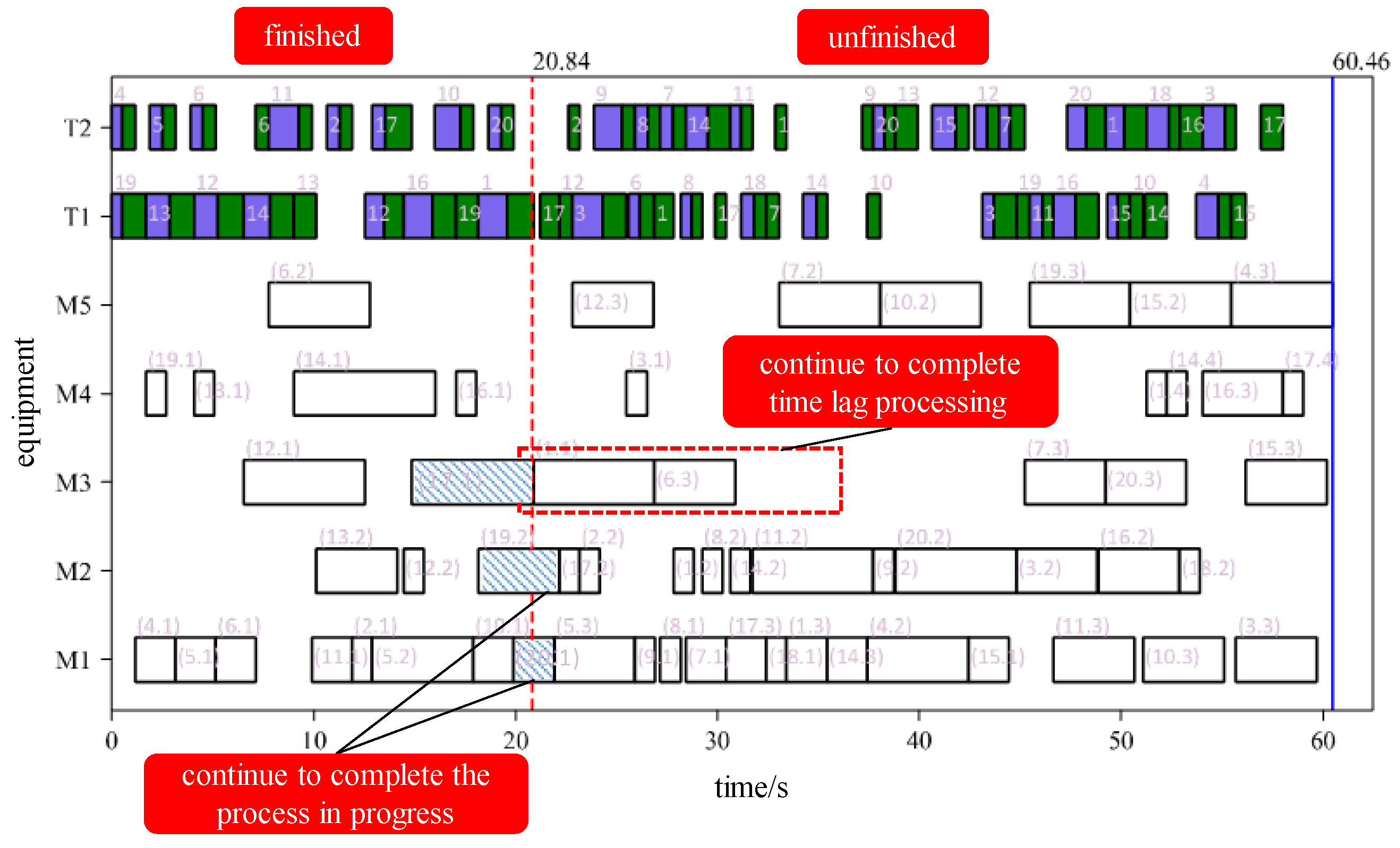
Figure 17.
Rescheduling results triggered by processing time lag disturbance.
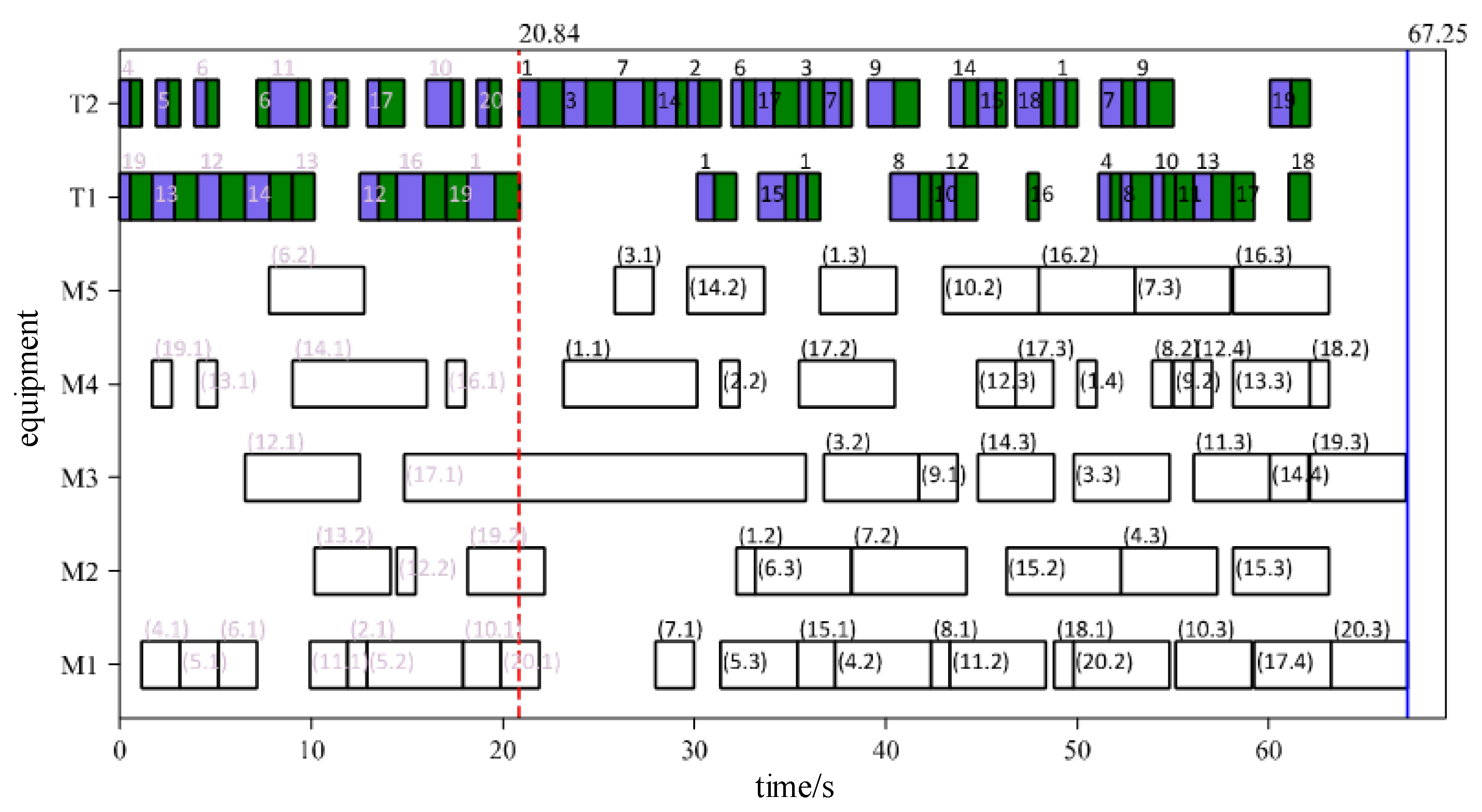
Figure 18.
Gantt chart of equipment scheduling plan for 40 jobs.
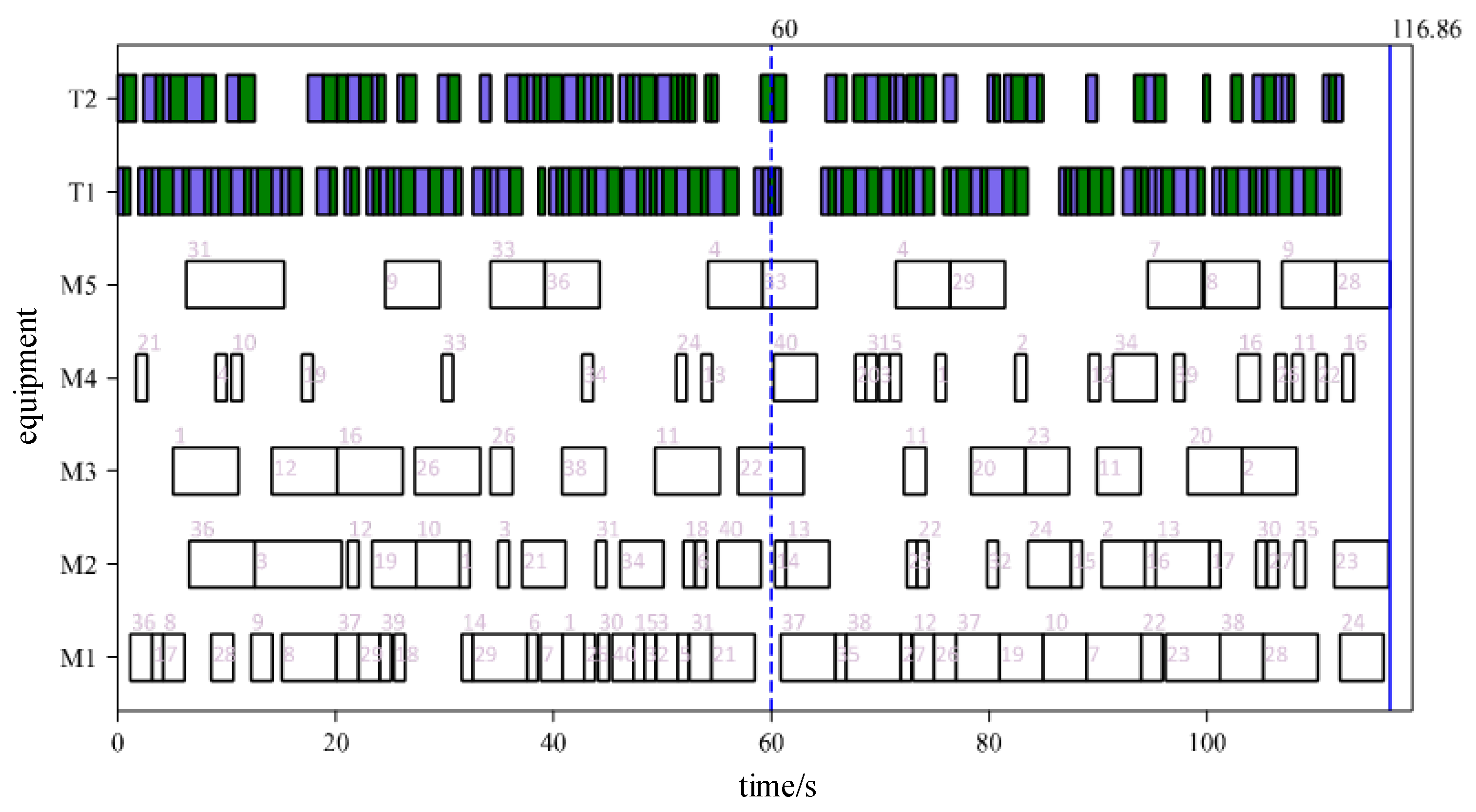
Figure 19.
Rescheduling results triggered by order disturbance.
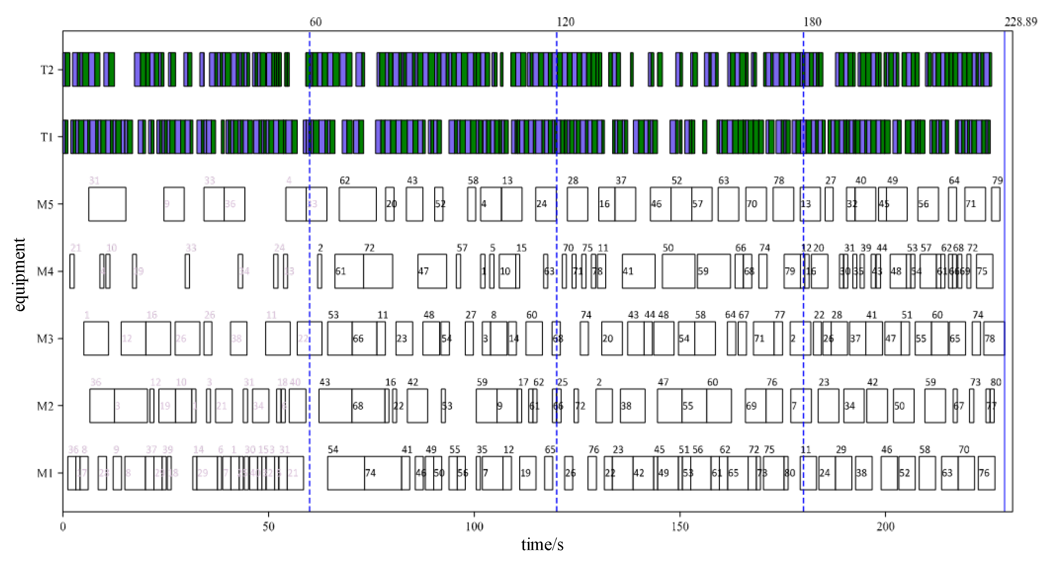

Table 1.
Operation selection rules.
| Number | Rule | Description |
| 1 | SRPT | Prioritize the job with the shortest remaining processing time. |
| 2 | SSO | Prioritize the job with the shortest processing time for the next process. |
| 3 | SRM | Prioritize the job with the shortest remaining processing time except for the current process. |
| 4 | MOP | Prioritize the job with the most remaining processes. |
| 5 | SOTCS | Prioritize the job with the smallest time progress under the current task arrangement. |
| 6 | SOP | Prioritize the job with the minimum number of processes |
Table 2.
Processing times of Kacem 4×5.
| job | process | Processing time | ||||
| M1 | M2 | M3 | M4 | M5 | ||
| J1 | O(1,1) | 2 | 5 | 4 | 1 | 2 |
| O(1,2) | 5 | 4 | 5 | 7 | 5 | |
| O(1,3) | 4 | 5 | 5 | 4 | 5 | |
| J2 | O(2,1) | 2 | 5 | 4 | 7 | 8 |
| O(2,2) | 5 | 6 | 9 | 8 | 5 | |
| O(2,3) | 4 | 5 | 4 | 54 | 5 | |
| J3 | O(3,1) | 9 | 8 | 6 | 7 | 9 |
| O(3,2) | 6 | 1 | 2 | 5 | 4 | |
| O(3,3) | 2 | 5 | 4 | 2 | 4 | |
| O(3,4) | 4 | 5 | 2 | 1 | 5 | |
| J4 | O(4,1) | 1 | 5 | 2 | 4 | 12 |
| O(4,2) | 5 | 1 | 2 | 1 | 2 | |
Table 3.
Transportation time of Kacem 4×5.
| Area nodes | A-area | B-area | F-area | M1 | M2 | M3 | M4 | M5 |
| A-area | 0 | 0.52 | 0.53 | 1.39 | 0.74 | 1.01 | 0.91 | 0.89 |
| B-area | 0.52 | 0 | 0.86 | 0.63 | 1.41 | 1.3 | 1.18 | 1.5 |
| F-area | 0.53 | 0.86 | 0 | 0.72 | 0.76 | 0.57 | 0.68 | 0.96 |
| M1 | 1.39 | 0.63 | 0.72 | 0 | 0.54 | 0.94 | 1.1 | 0.63 |
| M2 | 0.74 | 1.41 | 0.76 | 0.54 | 0 | 0.96 | 1.12 | 0.65 |
| M3 | 1.01 | 1.3 | 0.57 | 0.94 | 0.96 | 0 | 1.31 | 0.72 |
| M4 | 0.91 | 1.18 | 0.68 | 1.1 | 1.12 | 1.31 | 0 | 0.57 |
| M5 | 0.89 | 1.5 | 0.96 | 0.63 | 0.65 | 0.72 | 0.57 | 0 |
Table 4.
Comparative experimental results of the first five methods are for Kacem 4×5.
| Num | SRPT | LRPT | SSO | LSO | SRM | |||||
| Makespan | Decision time | Makespan | Decision time | Makespan | Decision time | Makespan | Decision time | Makespan | Decision time | |
| 1 | 156.21 | 0.11 | 57.08 | 0.09 | 148.46 | 0.05 | 164.81 | 0.06 | 140.84 | 0.09 |
| 2 | 151.03 | 0.11 | 58.04 | 0.11 | 154.52 | 0.05 | 169.19 | 0.06 | 149.97 | 0.09 |
| 3 | 131.05 | 0.11 | 54.84 | 0.09 | 129.73 | 0.05 | 152.44 | 0.06 | 132.75 | 0.08 |
| 4 | 169.15 | 0.12 | 65.14 | 0.12 | 145.12 | 0.06 | 179.05 | 0.06 | 152.69 | 0.09 |
| 5 | 113.37 | 0.08 | 54.69 | 0.09 | 118.63 | 0.05 | 113.13 | 0.05 | 99.96 | 0.08 |
| 6 | 155.86 | 0.13 | 65.06 | 0.12 | 161.71 | 0.05 | 186.47 | 0.08 | 152.96 | 0.09 |
| 7 | 192.78 | 0.13 | 60.31 | 0.12 | 184.62 | 0.06 | 176.43 | 0.06 | 171.25 | 0.13 |
| 8 | 168.52 | 0.12 | 68.41 | 0.14 | 161.4 | 0.06 | 180.13 | 0.06 | 166.6 | 0.12 |
| 9 | 149.34 | 0.11 | 59.35 | 0.11 | 149.14 | 0.06 | 147.48 | 0.05 | 132 | 0.09 |
| 10 | 162.61 | 0.12 | 63.33 | 0.11 | 167.29 | 0.06 | 160.6 | 0.06 | 162.56 | 0.11 |
| mean | 154.99 | 0.11 | 60.63 | 0.11 | 152.06 | 0.06 | 162.97 | 0.06 | 146.16 | 0.10 |
Table 5.
Comparative experimental results of the last five methods are for Kacem 4×5.
| Num | LRM | MOP | SOTCS | GA | DDQN | |||||
| Makespan | Decision time | Makespan | Decision time | Makespan | Decision time | Makespan | Decision time | Makespan | Decision time | |
| 1 | 65.34 | 0.09 | 56.68 | 0.02 | 55.79 | 0.02 | 57.13 | 64.74 | 55.86 | 2.91 |
| 2 | 64.32 | 0.09 | 57.53 | 0.03 | 57.75 | 0.02 | 69.65 | 63.87 | 58.93 | 1.77 |
| 3 | 63.3 | 0.09 | 61.82 | 0.02 | 56.31 | 0.02 | 50.38 | 62.65 | 60.86 | 1.81 |
| 4 | 67.79 | 0.11 | 62.45 | 0.02 | 59.47 | 0.02 | 61.39 | 65.17 | 58.55 | 1.81 |
| 5 | 63.2 | 0.08 | 53.62 | 0.02 | 55.08 | 0.02 | 53.73 | 58.73 | 54.3 | 1.73 |
| 6 | 74.05 | 0.11 | 62.69 | 0.03 | 62.18 | 0.02 | 64.23 | 66.65 | 60.61 | 1.86 |
| 7 | 68.37 | 0.11 | 64.26 | 0.02 | 60.65 | 0.03 | 61.72 | 67.59 | 64.26 | 2 |
| 8 | 68.94 | 0.12 | 63.8 | 0.02 | 66.48 | 0.03 | 66.69 | 68.57 | 64.18 | 1.91 |
| 9 | 64.86 | 0.09 | 58.07 | 0.02 | 57.66 | 0.02 | 57.89 | 64.26 | 58.07 | 1.86 |
| 10 | 71.17 | 0.11 | 65.45 | 0.03 | 61.31 | 0.02 | 71.72 | 66.6 | 63.07 | 1.91 |
| mean | 67.13 | 0.10 | 60.64 | 0.02 | 59.27 | 0.02 | 61.45 | 64.88 | 59.87 | 1.96 |
Table 6.
Comparative experimental results of the first five methods are for Kacem 8×8.
| Num | SRPT | LRPT | SSO | LSO | SRM | |||||
| Makespan | Decision time | Makespan | Decision time | Makespan | Decision time | Makespan | Decision time | Makespan | Decision time | |
| 1 | 247.34 | 0.23 | 83.18 | 0.22 | 250.39 | 0.11 | 228.8 | 0.09 | 170.16 | 0.19 |
| 2 | 228.54 | 0.19 | 76.14 | 0.21 | 228.98 | 0.11 | 221.78 | 0.09 | 170.66 | 0.17 |
| 3 | 270.24 | 0.22 | 82.09 | 0.23 | 213.63 | 0.12 | 210.74 | 0.11 | 145.51 | 0.2 |
| 4 | 231.66 | 0.22 | 78.95 | 0.23 | 255.65 | 0.12 | 215.54 | 0.09 | 174.6 | 0.2 |
| 5 | 223.28 | 0.19 | 68.52 | 0.17 | 206.65 | 0.09 | 198.99 | 0.09 | 146.88 | 0.16 |
| 6 | 228.08 | 0.2 | 71.64 | 0.21 | 232.6 | 0.12 | 218.5 | 0.09 | 161.94 | 0.19 |
| 7 | 196.57 | 0.17 | 72.46 | 0.19 | 201.25 | 0.09 | 199.24 | 0.09 | 159.63 | 0.16 |
| 8 | 218.81 | 0.2 | 74.35 | 0.19 | 244.48 | 0.09 | 202.4 | 0.09 | 154.55 | 0.17 |
| 9 | 263.9 | 0.2 | 73.71 | 0.2 | 272.66 | 0.11 | 211.3 | 0.09 | 169.7 | 0.18 |
| 10 | 206.19 | 0.19 | 68.89 | 0.17 | 212.58 | 0.09 | 217.01 | 0.09 | 147.62 | 0.16 |
| mean | 231.46 | 0.20 | 74.99 | 0.20 | 231.89 | 0.11 | 212.43 | 0.09 | 160.13 | 0.18 |
Table 7.
Comparative experimental results of the last five methods are for Kacem 8×8.
| Num | LRM | MOP | SOTCS | GA | DDQN | |||||
| Makespan | Decision time | Makespan | Decision time | Makespan | Decision time | Makespan | Decision time | Makespan | Decision time | |
| 1 | 109.48 | 0.2 | 71.43 | 0.03 | 65.17 | 0.05 | 74.97 | 79.52 | 104.06 | 3.59 |
| 2 | 107.1 | 0.2 | 69.37 | 0.03 | 73.03 | 0.03 | 70.41 | 79.5 | 102.24 | 2.33 |
| 3 | 116.59 | 0.21 | 72.84 | 0.04 | 75.52 | 0.03 | 72.63 | 83.98 | 104.43 | 2.56 |
| 4 | 106.62 | 0.19 | 72.4 | 0.03 | 77.58 | 0.05 | 72.07 | 78.69 | 99.96 | 2.45 |
| 5 | 97.29 | 0.16 | 68.93 | 0.05 | 68.72 | 0.03 | 65.04 | 74.49 | 89.48 | 2.46 |
| 6 | 101.72 | 0.2 | 74.83 | 0.03 | 70.78 | 0.03 | 73.12 | 79.82 | 101.89 | 2.45 |
| 7 | 105.99 | 0.16 | 71.7 | 0.03 | 70.93 | 0.03 | 64.96 | 70.33 | 99.71 | 2.03 |
| 8 | 107.5 | 0.17 | 69.35 | 0.03 | 69.34 | 0.04 | 76.05 | 75.64 | 101.96 | 2.32 |
| 9 | 114.72 | 0.17 | 73.73 | 0.04 | 70.82 | 0.03 | 74.98 | 79.44 | 108.14 | 2.41 |
| 10 | 107.32 | 0.16 | 65.61 | 0.03 | 69.72 | 0.05 | 64.74 | 74.04 | 97.29 | 2.09 |
| mean | 107.43 | 0.18 | 71.02 | 0.03 | 71.16 | 0.04 | 70.90 | 77.55 | 100.92 | 2.47 |
Table 8.
Comparative experimental results of the first five methods are for Kacem 10×10.
| Num | SRPT | LRPT | SSO | LSO | SRM | |||||
| Makespan | Decision time | Makespan | Decision time | Makespan | Decision time | Makespan | Decision time | Makespan | Decision time | |
| 1 | 172.04 | 0.36 | 63.91 | 0.35 | 166.8 | 0.19 | 155.84 | 0.16 | 129.46 | 0.27 |
| 2 | 161.56 | 0.34 | 64.16 | 0.36 | 166.16 | 0.19 | 151.27 | 0.16 | 123.74 | 0.3 |
| 3 | 152.47 | 0.39 | 63.28 | 0.36 | 159.53 | 0.19 | 163.55 | 0.16 | 142.7 | 0.28 |
| 4 | 182.51 | 0.39 | 64.89 | 0.38 | 153.71 | 0.16 | 142.55 | 0.17 | 116.59 | 0.29 |
| 5 | 164.1 | 0.37 | 64.6 | 0.37 | 179.39 | 0.17 | 162.22 | 0.16 | 148.13 | 0.28 |
| 6 | 167.6 | 0.39 | 58.36 | 0.37 | 160.16 | 0.17 | 145.78 | 0.16 | 122.6 | 0.31 |
| 7 | 165.72 | 0.36 | 61.54 | 0.37 | 155 | 0.19 | 145.22 | 0.16 | 127.99 | 0.3 |
| 8 | 174.16 | 0.37 | 61.4 | 0.37 | 175.68 | 0.17 | 163.88 | 0.16 | 131.2 | 0.28 |
| 9 | 147.5 | 0.38 | 60.86 | 0.35 | 156.91 | 0.17 | 141.91 | 0.14 | 119.37 | 0.28 |
| 10 | 165.95 | 0.38 | 62.75 | 0.37 | 170.97 | 0.17 | 159.59 | 0.17 | 117.67 | 0.28 |
| mean | 165.36 | 0.37 | 62.58 | 0.37 | 164.43 | 0.18 | 153.18 | 0.16 | 127.95 | 0.29 |
Table 9.
Comparative experimental results of the last five methods are for Kacem 10×10.
| Num | LRM | MOP | SOTCS | GA | DDQN | |||||
| Makespan | Decision time | Makespan | Decision time | Makespan | Decision time | Makespan | Decision time | Makespan | Decision time | |
| 1 | 96.62 | 0.28 | 60.51 | 0.03 | 61.42 | 0.05 | 60.3 | 68.09 | 63.46 | 3.19 |
| 2 | 91.61 | 0.3 | 62.25 | 0.03 | 61.33 | 0.05 | 59.21 | 65.21 | 54.27 | 2.01 |
| 3 | 89.89 | 0.28 | 59.87 | 0.05 | 61.85 | 0.05 | 58.11 | 64.2 | 57.79 | 2.12 |
| 4 | 92.78 | 0.29 | 60.71 | 0.03 | 62.84 | 0.05 | 59.54 | 65.7 | 59.82 | 2.05 |
| 5 | 81.32 | 0.28 | 60.1 | 0.05 | 60.1 | 0.03 | 57.88 | 65.36 | 61.79 | 2.12 |
| 6 | 88.72 | 0.31 | 59.06 | 0.05 | 55.53 | 0.05 | 59.22 | 66.9 | 60.53 | 1.99 |
| 7 | 92.54 | 0.3 | 61.58 | 0.05 | 59.95 | 0.03 | 60.03 | 66.05 | 60.39 | 2.07 |
| 8 | 83.24 | 0.28 | 59.24 | 0.05 | 60.14 | 0.03 | 60.37 | 64.23 | 60.16 | 2.05 |
| 9 | 91.49 | 0.28 | 59.7 | 0.05 | 60.46 | 0.05 | 59.81 | 63.68 | 57.01 | 2.12 |
| 10 | 94.51 | 0.28 | 63.91 | 0.05 | 60.04 | 0.03 | 60.3 | 63.24 | 59.95 | 1.99 |
| mean | 90.27 | 0.29 | 60.69 | 0.04 | 60.37 | 0.04 | 59.48 | 65.27 | 59.52 | 2.17 |
Table 10.
Comparative experimental results of the first five methods are for Kacem 15×10.
| Num | SRPT | LRPT | SSO | LSO | SRM | |||||
| Makespan | Decision time | Makespan | Decision time | Makespan | Decision time | Makespan | Decision time | Makespan | Decision time | |
| 1 | 245.74 | 0.31 | 64.68 | 0.32 | 233.17 | 0.14 | 258.42 | 0.14 | 246.22 | 0.26 |
| 2 | 229.09 | 0.3 | 65.88 | 0.31 | 251.46 | 0.13 | 219.77 | 0.14 | 223.66 | 0.26 |
| 3 | 246.62 | 0.31 | 66.8 | 0.34 | 232.11 | 0.14 | 226.67 | 0.15 | 225.67 | 0.27 |
| 4 | 235.26 | 0.3 | 63.01 | 0.38 | 230.31 | 0.16 | 229.66 | 0.14 | 232.9 | 0.25 |
| 5 | 246.83 | 0.3 | 66.03 | 0.32 | 223.03 | 0.14 | 274.89 | 0.15 | 231.66 | 0.25 |
| 6 | 203.07 | 0.24 | 60.35 | 0.24 | 222.43 | 0.11 | 213.72 | 0.12 | 208.09 | 0.2 |
| 7 | 239.91 | 0.25 | 65.28 | 0.27 | 241.67 | 0.12 | 237.86 | 0.13 | 220.97 | 0.22 |
| 8 | 234.85 | 0.27 | 61 | 0.29 | 224.97 | 0.12 | 251.74 | 0.13 | 229.91 | 0.24 |
| 9 | 238.56 | 0.29 | 66.49 | 0.31 | 231.1 | 0.14 | 225.6 | 0.14 | 239.51 | 0.25 |
| 10 | 211.35 | 0.29 | 68.06 | 0.31 | 232.91 | 0.14 | 224.79 | 0.14 | 203.81 | 0.26 |
| mean | 233.13 | 0.29 | 64.76 | 0.31 | 232.32 | 0.13 | 236.31 | 0.14 | 226.24 | 0.25 |
Table 11.
Comparative experimental results of the last five methods are for Kacem 15×10.
| Num | LRM | MOP | SOTCS | GA | DDQN | |||||
| Makespan | Decision time | Makespan | Decision time | Makespan | Decision time | Makespan | Decision time | Makespan | Decision time | |
| 1 | 80.81 | 0.3 | 62.01 | 0.05 | 59.35 | 0.05 | 67.11 | 92.59 | 68.42 | 5.62 |
| 2 | 74.77 | 0.29 | 65.36 | 0.05 | 61.1 | 0.05 | 61.73 | 89.09 | 62.21 | 2.72 |
| 3 | 74.88 | 0.3 | 63.6 | 0.05 | 67.66 | 0.05 | 70.19 | 88.94 | 69.81 | 3.06 |
| 4 | 77.52 | 0.28 | 62.67 | 0.05 | 56.78 | 0.06 | 65.26 | 88.19 | 64.86 | 2.71 |
| 5 | 76.11 | 0.28 | 66.23 | 0.05 | 63.27 | 0.05 | 64.05 | 89.53 | 61 | 2.67 |
| 6 | 74.56 | 0.21 | 56.59 | 0.04 | 62.57 | 0.04 | 56.3 | 78.88 | 60.35 | 2.35 |
| 7 | 78.76 | 0.24 | 61.04 | 0.04 | 64.51 | 0.04 | 61.76 | 84.1 | 69.94 | 2.52 |
| 8 | 83.08 | 0.27 | 63.56 | 0.05 | 62.81 | 0.05 | 65.11 | 86.5 | 65.86 | 2.71 |
| 9 | 75.1 | 0.28 | 65.34 | 0.05 | 66.66 | 0.05 | 59.67 | 84.73 | 67.2 | 2.58 |
| 10 | 75.89 | 0.28 | 64.05 | 0.05 | 69.86 | 0.05 | 62.42 | 87.41 | 65.69 | 2.69 |
| mean | 77.15 | 0.27 | 63.05 | 0.05 | 63.46 | 0.05 | 63.36 | 87.00 | 65.53 | 2.96 |
Disclaimer/Publisher’s Note: The statements, opinions and data contained in all publications are solely those of the individual author(s) and contributor(s) and not of MDPI and/or the editor(s). MDPI and/or the editor(s) disclaim responsibility for any injury to people or property resulting from any ideas, methods, instructions or products referred to in the content. |
© 2024 by the authors. Licensee MDPI, Basel, Switzerland. This article is an open access article distributed under the terms and conditions of the Creative Commons Attribution (CC BY) license (http://creativecommons.org/licenses/by/4.0/).
Copyright: This open access article is published under a Creative Commons CC BY 4.0 license, which permit the free download, distribution, and reuse, provided that the author and preprint are cited in any reuse.


