
Submitted:
16 May 2025
Posted:
27 May 2025
You are already at the latest version
Abstract
This study presents a reinforcement learning–based approach to optimize replenishment policies in the presence of uncertainty, with the objective of minimizing total costs, including inventory holding, shortage, and ordering costs. The focus is on single-level assembly systems, where both component delivery lead times and finished product demand are subject to randomness. The problem is formulated as a Markov Decision Process (MDP), in which an agent determines optimal order quantities for each component by accounting for stochastic lead times and demand variability. A Deep Q-Network (DQN) algorithm is adapted and employed to learn optimal replenishment policies over a fixed planning horizon. To enhance learning performance, we develop a tailored simulation environment that captures multi-component interactions, random lead times, and variable demand, along with a modular and realistic cost structure. The environment enables dynamic state transitions, lead time sampling, and flexible order reception modeling, providing a high-fidelity training ground for the agent. To further improve convergence and policy quality, we incorporate local search mechanisms and multiple action space discretizations per component. Experimental results show that the proposed method significantly reduces stockouts and overall costs while improving the system’s adaptability to uncertainty. These findings highlight the potential of deep reinforcement learning as a data-driven and dynamic approach to inventory management in complex and uncertain supply chain environments.
Keywords:
Keywords: Assembly system
; Inventory management
; Replenishment Planning
; Stochastic demand
; Uncertain lead times
; Deep Reinforcement learning
; Deep Q-Network (DQN)
; Data-driven inventory management
1. Introduction
In the context of supply chain and inventory management, planning plays a critical role in the effectiveness of replenishment strategies [1]. Well-designed planning processes help maintain optimal inventory levels, balancing the risk of overstocking—which leads to increased storage costs—with the risk of stockouts, which can cause lost sales and diminished customer satisfaction [2]. By ensuring the timely availability of products, components, or raw materials to meet production schedules or customer demand, effective planning contributes directly to improved service levels and enhanced customer loyalty [3]. These challenges are further compounded under conditions of uncertainty, where variability in demand and supplier lead times can significantly disrupt replenishment decisions.
In replenishment management, planning is essential to maintaining a balance between supply and demand, minimizing costs, and ensuring customer satisfaction [4]. Effective planning enables the optimal implementation of replenishment policies [5], aligning inventory decisions with strategic business objectives such as cost reduction and high product availability. These policies adjust order quantities and stock levels based on real-time market conditions. The effectiveness of such planning depends largely on its ability to adapt to various sources of uncertainty arising from collaborative operations between manufacturers and customers, interactions with suppliers of raw materials or critical components, and even internal manufacturing processes [6]. The nature of this uncertainty is multifaceted [7], often resulting in increased operational costs, reduced profitability, and diminished customer satisfaction [8]. Numerous studies emphasize key sources of uncertainty in manufacturing environments, including demand variability, fluctuations in supplier lead times, quality issues, and capacity constraints [9].
Demand uncertainty significantly impacts supply chain design. While stochastic programming models outperform deterministic approaches in optimizing strategic and tactical decisions [10], most studies overlook lead time variability caused by real-world disruptions. Companies typically address supply uncertainty through safety stocks and safety lead times [11], which trade off shortage risks against higher inventory costs. The key challenge lies in finding the optimal balance between these competing costs. For a long time, lead time uncertainty received relatively little attention in the literature, with most research in inventory management focusing predominantly on demand uncertainty [12]. In assembly systems, component lead times are often subject to uncertainty; they are rarely deterministic and typically exhibit variability [13].
The literature on stochastic lead times in assembly systems has seen significant contributions that have shaped current approaches to inventory control under uncertainty[14]. A notable study by [15] investigates a single-level assembly system under the assumptions of stochastic lead times, fixed and known demand, unlimited production capacity, a lot-for-lot policy, and a multi-period dynamic setting. In this work, lead times are modeled as independent and identically distributed (i.i.d.) discrete random variables. The authors focus on optimizing inventory policies by balancing component holding costs and backlogging costs for finished products, ultimately deriving optimal safety stock levels when all components share identical holding costs. This problem is further extended in [16], which considers a different replenishment strategy—the Periodic Order Quantity (POQ) policy. In [17], the lot-for-lot policy is retained but a service level constraint is introduced. A Branch and Bound algorithm is employed to manage the combinatorial complexity associated with lead time variability. Subsequent studies [18,19], and [20] build on this foundation by refining models to better capture lead time uncertainty in single-level assembly systems, while also proposing extensions to multi-level systems and providing a more detailed analysis of the trade-offs between holding and backlogging costs.
Modeling multi-product, multi-component assembly systems under demand uncertainty is inherently complex. [21] proposes a modular framework for supply planning optimization, though its effectiveness depends on computational reductions and assumptions about probability distributions. For Assembly-to-Order systems, [22] develops a cost-minimization model incorporating lead time uncertainty, solved via simulated annealing. Several studies [23,24,25] and [26] address single-period supply planning for two-level assembly systems with stochastic lead times and fixed end-product demand. Using Laplace transforms, evolutionary algorithms, and multi-objective methods, they optimize component release dates and safety lead times to minimize total expected costs (including backlogging and storage costs). [2] later improved upon [18]’s work, while [27] extended the framework to multi-level systems under similar assumptions.
Existing models often rely on oversimplified assumptions about delivery times and demand, limiting their practical applicability [21]. This highlights the need for new optimization frameworks that better capture real-world complexities and component interdependencies in assembly systems. We enhance [15]’s method by incorporating : (1) stochastic demand models, (2) ordering and stockout penalty costs, and (3) MDP-based stochastic modeling. Deep reinforcement learning techniques, are employed to optimize solutions under delivery and demand uncertainties.
Over the years, various modeling approaches have been proposed to address uncertainty [28], including: Conceptual models: Theoretical approaches to understand the relationships between variables, Analytical models: use of mathematical formulas to optimize decisions, Simulations: reproduction of system behavior to test different policies and Artificial intelligence: use of algorithms to predict and optimize decisions. The choice of approach depends on key characteristics of the manufacturing context.
Production Planning and Control (PPC) must combine rigorous planning with technological flexibility to adapt to the complex dynamics of supply chains [29]. The integration of artificial intelligence (AI), such as reinforcement learning (RL), and digital tools is now essential to achieve these objectives[30]. This trend aligns with Industry 4.0, where AI and machine learning play a central role in improving industrial efficiency. Industry 4.0 represents a major transformation in production systems, and PPC is evolving toward self-managing systems that combine automation (e.g., robots and smart sensors) with decision-making autonomy (e.g., AI and machine learning) [29]. This paper [31] presents a systematic review of 181 scientific articles exploring the application of reinforcement learning (RL) techniques in PPC. It provides a mapping of RL applications across five key areas of PPC: Resource planning, capacity planning, purchasing and supply management, production scheduling and Inventory Management.
This study develops a discrete inventory optimization model for single-level assembly systems (multi-component, multi-period) under stochastic conditions. Overcoming existing limitations, we: Integrate multiple logistics costs,Relax restrictive assumptions (uniform delivery distributions, fixed demand, uniform storage costs), introduce component-based stockout calculation, employ deep reinforcement learning for efficient implementation. The model features integer decision variables for MRP compatibility while addressing dual uncertainties (demand/delivery). Current scope remains assembly-level systems. The problem involves optimizing replenishment policies under uncertainty. We chose to use a Deep Q-Network (DQN) algorithm, a Deep Reinforcement Learning (DRL) approach that learns an optimal replenishment policy through interactions with the environment. We avoid traditional optimization methods because they are often unsuitable for inventory management problems with uncertain delivery times and stochastic demand [32].
The first challenge in optimizing replenishment policies under uncertainty lies in the inadequacy of classical optimization methods. We chose to use a Deep Q-Network (DQN) algorithm, a Deep Reinforcement Learning (DRL) approach that learns an optimal replenishment policy through interactions with the environment. We avoid traditional optimization methods because they are often unsuitable for inventory management problems with uncertain delivery times and stochastic demand [32]. Overly Simplistic Assumptions: Classical methods (e.g., deterministic or stochastic optimization) typically assume that problem parameters—such as delivery times and demand—are either deterministic or follow simple, easily exploitable distributions [33]. However, in real-world scenarios, delivery times are often random with complex probability distributions, making classical modeling approaches highly impractical. Adaptability to Uncertainty: Unlike traditional methods, DQN does not require explicit modeling of distributions. Instead, it dynamically adapts to uncertainties by learning from experience, making it more robust in stochastic environments.
The second challenge lies in the complexity and high dimensionality of the problem, which involves multiple dynamic factors: time-varying inventory levels, uncertain delivery times, stochastic demand, and multiple cost structures (e.g., holding, shortage, and ordering costs). Traditional optimization methods struggle with such complexity: Linear Programming (LP) becomes inapplicable due to the explosion of variables and constraints in realistic scenarios [34]. Classical Dynamic Programming (DP) suffers from the curse of dimensionality [35], as it requires storing and computing excessively large value tables [36]. These limitations motivate the use of Deep Q-Networks (DQN) [37], which leverage neural networks to approximate the function efficiently. Unlike DP, DQN avoids explicit state enumeration and instead generalizes across states, making it scalable to high-dimensional problems [38].
The third critical aspect involves the system’s dynamics and adaptability requirements in real industrial environments, where practical challenges emerge such as fluctuating periodic demand and unpredictable delivery times, necessitating dynamic decision-making. Traditional models prove inadequate for these scenarios as they typically employ static approaches or require computationally intensive re-optimization processes [39]. In contrast, the Deep Q-Network (DQN) framework dynamically adapts its policy through continuous learning from system observations, enabling it to develop optimal sequential decision strategies that effectively minimize long-term operational costs without explicit re-optimization [40].
This paper is organized as follows: Section 1 provides an introduction to the research context and outlines relevant work in supply planning under uncertainty, emphasizing key challenges and gaps in existing approaches. Section 2 describes the problem in detail, including the characteristics of the inventory environment and the sources of uncertainty. Section 3 presents the proposed methodology, including the formulation of the problem as a Markov Decision Process (MDP). Section 4 introduces the Deep Q-Network (DQN) algorithm and explains its implementation for learning optimal replenishment policies. Section 5 discusses the experimental results and provides an analysis of the findings. Finally, Section 6 concludes the paper by summarizing the main contributions, acknowledging limitations, and suggesting directions for future research.
2. Problem Description
Replenishment planning in single-level assembly systems under stochastic demand and lead time uncertainty presents a complex optimization problem where component orders must be determined amid two key sources of variability: (1) uncertain demand for the finished product, and (2) random lead times for each component. The core optimization challenge involves minimizing the total expected costs comprising inventory holding costs, stockout penalties and ordering costs. Crucially, demand follows a known probability distribution, while each component’s lead time is characterized by its own distinct distribution. These stochastic elements create a cascading risk effect - the failure to secure any single component due to lead time variability can halt the entire assembly process. The fundamental objective is to develop an optimal ordering strategy that achieves robust system performance while maintaining cost efficiency under uncertainty, requiring careful consideration of both demand-side and supply-side stochasticity in an integrated framework.
Figure 1 illustrates a single-level Bill of Materials (BOM) for an assembly system, depicting the relationship between a finished product (FP) and its components (i1, i2, ..., in). The diagram shows that one unit of FP is assembled from multiple components, each with a specific consumption coefficient (ci), representing the quantity required per unit of FP.
3. Methodology
To model the replenishment planning problem under lead-time uncertainty as a reinforcement learning (RL) task, we formulate it as a Markov Decision Process (MDP). The MDP framework captures the dynamics of inventory management, where the agent makes decisions on ordering and stock management at each time step. The reward function is designed to incorporate key cost components, including storage costs for each component, the shortage cost of finished products, penalties for stockouts of components, and the ordering costs associated with replenishment decisions.
3.1. MDP Environment
The environment in a Markov Decision Process (MDP) is everything external to the agent. It defines how the world responds to the agent’s actions and evolves over time.
Structure of the Environment
At each time step t:
- The agent observes the current state .
- It chooses an action .
-
The environment responds:
- –
- It transitions to a new state .
- –
- It emits a reward .

Table 1.
List of Variables and Notations.
| Symbol | Description |
|---|---|
| PF | Finished product. |
| i | component. |
| t | Period. |
| Random demand for finished products at period t, modeled as a stochastic variable with a known probability distribution. | |
| Delivery time of component i ordered at period t, a random variable with a known probability distribution. | |
| Quantity ordered of component i at period t. | |
| Stock level of component i at the end of period t. | |
| Quantity of component i received at period t. | |
| Quantity of component i needed to produce one unit of finished product (consumption coefficient ). | |
| Unit holding cost per period for component i. | |
| Unit shortage cost for component i. | |
| Empty stock cost for component i. | |
| Order placement cost for component i. | |
| M | Maximum order quantity permitted for each component per period. |
| T | Planning horizon (number of periods). |
| N | Number of components needed to assemble the finished product. |
| Space of actions. | |
| Space of states. |
Figure 2 represents a reinforcement learning process or a dynamic decision-making system in the context of inventory management. It is divided into four main components, arranged in a circular flow to illustrate the sequence of steps in the process. Each component is represented by a colored circle, and the transitions between them are shown with curved arrows.
States
The state of the system can be represented by a vector of the current stock levels for all components i.
Actions
An action represents the decisions regarding the quantities to be ordered at each period t. Each corresponds to the quantity ordered for each component at the beginning of the period.
This is the vector of quantities ordered for each component i at period . denotes the initial action space (discrete values). Each component i can take any value in the interval . To ensure that the algorithm adjusts ordered quantities based on the specific characteristics of each component and avoids restricted or similar order quantities, it is important to define a flexible action space. A poorly defined action space (i.e., limited or uniform order quantities) could reduce the algorithm’s adaptability.
To address this, we dynamically adjust the action range for each component, ensuring sufficient diversity in possible order quantities. This allows the algorithm to adapt orders based on each component’s specific needs.
If the action space were too limited or similar across components, the algorithm might lack the flexibility needed to optimize orders effectively. To prevent this, we assign different quantity ranges to each component based on its importance. Instead of using a fixed set of possible actions, we adapt order ranges according to consumption coefficients and maximum delivery times. Components with higher consumption and longer delivery times have wider action ranges, allowing the algorithm to order more or less as needed. This flexibility enhances the algorithm’s ability to optimize stock management.
So to adjust the action space for each component based on its consumption coefficient and maximum delivery time, it is useful to dynamically adapt the action space according to the consumption of each component and its delivery period ().
Scaling the Action Space
The more a component is consumed and the longer it takes to be delivered, the larger its action range should be for better stock management. This can be achieved by adjusting the upper limit of the action space for each component.
Action Space Modeling Logic
Instead of defining a fixed-size discrete space for each component (e.g., from 0 to ), we can implement an adaptive action space tailored to each component’s characteristics.
Action Space for a Component
with Estimated requirement =
This strategy is cautious, as it ensures that the model accounts for scenarios where demand is at its peak and delivery times are at their longest. By considering only the maximum demand and maximum delivery time, we prevent underestimating needs, even in extreme conditions, by creating an action space that includes all possible situations. In cases of overestimation, the agent will learn an optimal policy that naturally avoids unnecessary actions.
Global Action Space
where × represents the Cartesian product.
Transition Function
The expression of the transition function in a replenishment planning problem under uncertainty of random delivery times is used to describe how the state of the system evolves from one period to another, depending on the realizations of the random variables (delivery times), inventory levels, decisions already made (order quantities), and demand D.
Formally, the transition function can be written as
Inventory Level Formula
The inventory level for each component i at the end of period t is given by
- Let D be a random variable representing the demand for the finished product. It follows a discrete distribution on , with known associated probabilities:
- The random variable represents the delivery time of component ii, which follows a discrete probability distribution on the set with the associated probabilities:
Computation of Receipts
The quantity received is the sum of orders placed in previous periods that are delivered in period t.
- : An indicator function that is equal to 1 if the order for component i placed in period is delivered in period t and 0 otherwise, i.e. an indicator that is equal to 1 if the delivery time for the order for component i placed in period k is exactly equal , and 0 otherwise.
Reward Function
The reward for a period t is defined as the inverse of the total cost:
3.2. Storage Cost
Storage cost is the cost associated with maintaining component inventory in the warehouse. It is calculated based on the number of units of the components and the unit storage cost. The following formula calculates the storage cost associated with components .
-
: Represents the storage cost for each component when the stock level is positive.We add the storage costs of the components only if their stock levels are positive ( ), that is, if the components are in stock.
3.3. Shortage Cost
The cost of shortage is calculated based on the inventory levels of the components (based on the number of missing component units) and the shortage cost per component unit . The shortage cost is the cost associated with the lack of components needed to produce the finished product, which can lead to stockouts and lost sales. So the unavailability of components "component shortage" can lead to a disruption in the production of the finished product.
- : Represents the shortage cost for each component. This shortage is linked to the lack of component i, when its stock level is negative.
We therefore add the costs of component shortages, only if the stock is insufficient (), a negative stock level for a component i indicates an inability to satisfy the production of the finished product.
3.4. Empty Inventory Cost (Zero Inventory)
Empty inventory represents a situation where replenishment is needed quickly. It is not a complete shortage (because there is still time to react), but it is a situation that could quickly lead to a shortage. The inventory cost is defined by
3.5. Order Launch Cost
The order launch cost (or order placement cost) refers to all the expenses associated with issuing and processing an order. The order launch cost is paid each time an order of i is launched at t so if
3.6. Total Cost
3.7. Optimal Policy
A function that determines the optimal quantity to order in each period to minimize the expected total cost over horizon T :
The policy is a function that defines the quantity to order for each state Your objective is to find the policy that minimizes the expected total cost across all periods . So the policy defines how to choose the quantities to order based on the current state of the environment (e.g. current inventory levels, lead time probabilities, etc.).
Objective:
Minimize the cumulative reward function R over the planning horizon , which represents the total cost by adapting the ordering policy to minimize inventory and stockout costs. This model takes into account the stochastic demand for the finished product, random lead times of components with specified probability distributions, and seeks to determine the optimal order quantities to minimize inventory, stockout and order release costs.
4. DQN (Deep Q-Network)
Deep Reinforcement Learning (Deep RL) is a combination of Reinforcement Learning (RL) and Deep Neural Networks (Deep Learning) [41]. It allows an agent to learn optimal strategies in complex environments using powerful nonlinear approximations. Deep RL can solve complex problems (games, robotics, NLP) thanks to the power of deep networks. Major challenges (instability, divergence) have been partially addressed by techniques such as DQN [42].
4.1. Structure of the DQN Algorithm
The implemented Deep Q-Network (DQN) algorithm is structured around four core components. The first is the Replay Buffer, which stores past transitions in the form and enables the agent to learn from a randomized mini-batch of experiences, thereby reducing temporal correlation and stabilizing learning. The second component is the Q-Network, a feedforward neural network consisting of an input layer, a hidden layer with ReLU activations, and an output layer that approximates Q-values for each possible action. The third module is the DQN Agent, which initializes the Q-Network and Target Network, sets essential hyperparameters (e.g., learning rate, discount factor , and exploration rate ), and manages the optimization and interaction with the replay buffer. Finally, the Action Selection mechanism adopts an epsilon-greedy strategy to balance exploration and exploitation, selecting either a random action with probability or the action with the maximum estimated Q-value. This architecture provides a modular and efficient foundation for deep reinforcement learning in environments with discrete and multi-dimensional action spaces.
| Algorithm 1 Replay Buffer |
|
| Algorithm 2 Q-Network Forward Pass |
|
| Algorithm 3 DQN Agent |
|
| Algorithm 4 Select Action |
|
4.2. Comprehensive Comparison of Inventory Planning Methods
Table 2 compares classical models, optimization methods, machine learning approaches, and metaheuristics for inventory and replenishment planning.
Table 3 provides a comprehensive summary of the key parameters used in both the inventory environment and the Deep Q-Network (DQN) agent, outlining their values and respective roles in the learning and decision-making processes.
5. Results and Discussion
The environment parameters define the operational characteristics of the inventory system, such as the number of components, penalty and holding costs, demand and lead time uncertainties, and the structure of consumption. These parameters ensure the simulation accurately reflects the complexities of real-world supply chains. The agent parameters govern the learning process, including the neural network architecture, learning rate, exploration behavior, and training configuration. The inclusion of a replay buffer further enhances learning stability by breaking temporal correlations in the training data. The DQN algorithm is employed to learn optimal ordering policies over time. By interacting with the environment through episodes, the agent receives feedback in the form of rewards, which reflect the balance between minimizing shortage penalties and storage costs. To facilitate the simulation and make the analysis more interpretable, simple parameter values were used in the first table, including, limited lead time possibilities, and a small range of demand values. Additionally, the reward function was normalized (reward divided by 1000) to simplify numerical computations and stabilize the learning process. Despite this simplification, the implemented environment and reinforcement learning algorithms are fully generalizable: they can handle any number of components (n), multiple lead time scenarios, and a range of demand values (m), making the model adaptable to more complex and realistic settings. However, scaling up to larger instances requires significant computational resources, as the state and action spaces grow exponentially. Therefore, a powerful machine is recommended to run simulations efficiently when moving beyond the simplified test case.
The algorithm is developed using the Python programming language, which is particularly well-suited for research in reinforcement learning and operations management due to its expressive syntax and the availability of advanced scientific libraries. The implementation employs NumPy for efficient numerical computation, particularly for manipulating multidimensional arrays and performing vectorized operations that are essential for simulating the environment and computing rewards. Visualization of training performance and inventory dynamics is facilitated through Matplotlib, which provides robust tools for plotting time series and comparative analyses. The core reinforcement learning model is implemented using PyTorch, a state-of-the-art deep learning framework that supports dynamic computation graphs and automatic differentiation. PyTorch is used to construct and train the deep Q-network (DQN), manage the neural network architecture, optimize parameters through backpropagation, and handle experience replay to stabilize the learning process. Collectively, these libraries provide a powerful and flexible platform for modeling and solving complex inventory optimization problems under stochastic conditions.
Performance and Policy Evaluation
Figure 3 shows the evolution of rewards over training episodes. Initially, the agent exhibits high variability in performance due to random actions and limited experience. As training progresses, particularly after episode 100, the rewards stabilize and approach zero, indicating that the agent has learned a policy that effectively minimizes inventory-related costs.
Figure 4 illustrates the agent’s learned ordering policies over time. Early in training, the ordered quantities fluctuate significantly, reflecting exploration. Eventually, the policy converges toward more stable ordering behaviors. Component 2 is ordered most frequently and in larger quantities, suggesting its higher importance or greater risk of shortage. Component 3 is ordered less often, possibly due to lower consumption or more favorable lead times.
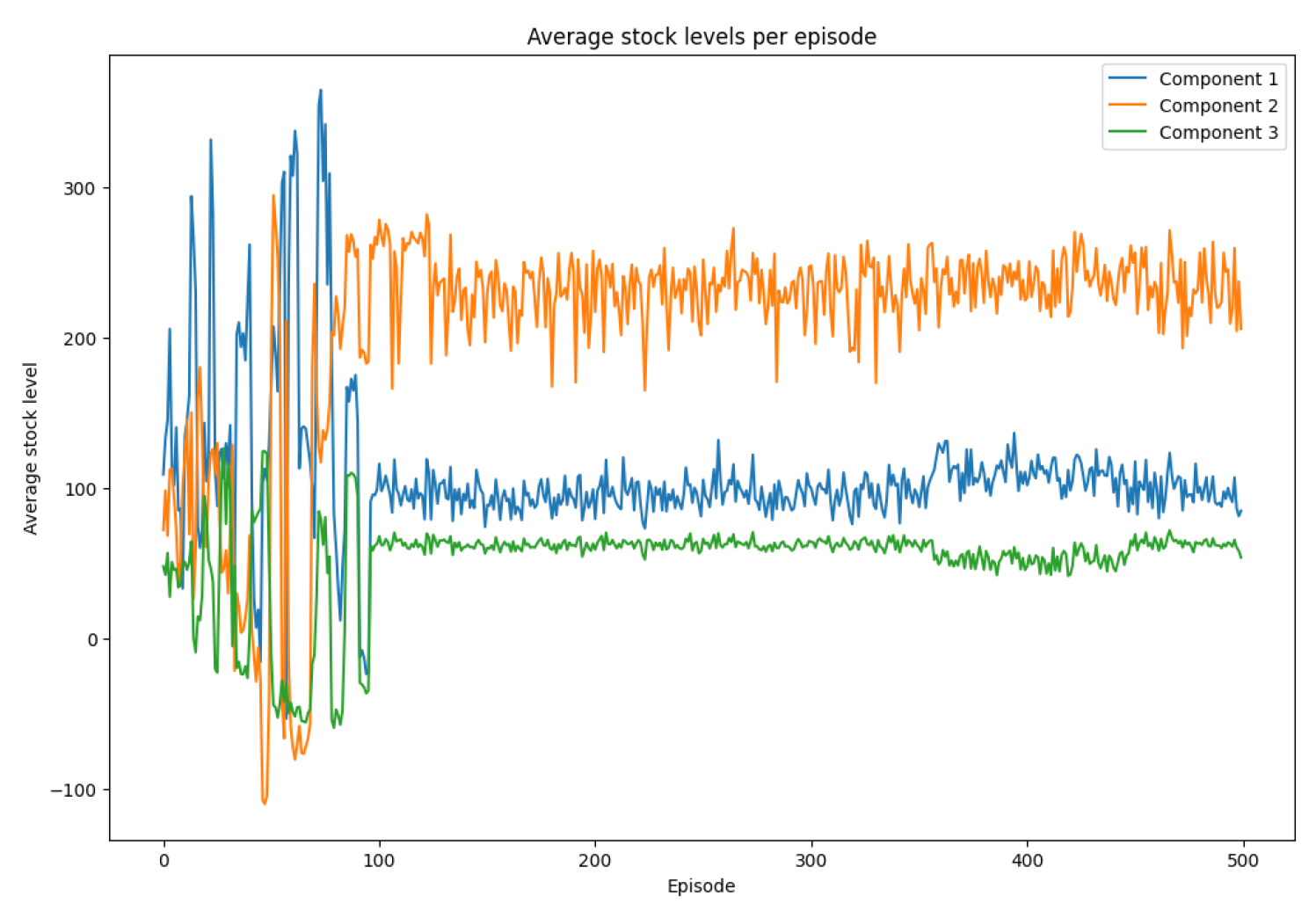
The evolution of average stock levels is presented in Figure 5. Initially, the stock levels are volatile and include frequent shortages (negative values). Over time, the agent learns to anticipate demand and lead times better, leading to smoother inventory levels. The final stock levels—higher for component 2—reflect its strategic importance and confirm the ordering strategy learned.
The results clearly demonstrate the capability of the DQN algorithm to adaptively optimize inventory policies under uncertainty. The convergence of rewards, the consistency in ordering patterns, and the stabilized stock levels collectively validate the effectiveness of the learning process.
Lead Time and Risk Analysis
The three components in the inventory system exhibit distinct patterns in both consumption and lead time variability, which significantly influence their associated risks. Component , with the highest consumption coefficient, demonstrates a relatively stable delivery profile: 80 % of its orders are fulfilled within 1 or 2 periods, making it the least risky in terms of delays. In contrast, Component , which has a moderate consumption rate of 2, faces greater uncertainty— 30% of its orders experience a delay of 3 periods, and 40% are delayed by 2 periods. This combination indicates a substantial risk of stockout if not managed carefully. Component , despite its lower consumption rate of 1, shares the same 30% probability of a 3-period delay as but has only a 10% chance of being delivered within 1 period, the lowest among all components. This makes the most vulnerable to supply disruptions. Overall, the risk of delivery delays is highest for , followed closely by , while remains the most reliable in terms of lead time performance.
5.1. Impact of Lead Times on Ordered Quantities
When a component has a longer and more uncertain lead time, the agent tends to adapt its ordering strategy to mitigate the risk of stockouts. This often results in placing orders more frequently in anticipation of potential delays. Additionally, the agent may choose to maintain a higher inventory level as a buffer, ensuring that production is not interrupted due to late deliveries.
Table 4 presents a detailed analysis of the relationship between each component’s consumption level, its lead time uncertainty, and the resulting ordering behavior by the agent. Components with higher consumption but more reliable lead times, such as , allow for stable and moderate ordering. In contrast, components like and especially , which are subject to longer and more uncertain delivery delays, require the agent to compensate by increasing order frequency . This strategic adjustment helps to avoid shortages despite the variability in supplier lead times. The table summarizes these insights for each component.
To better understand the agent’s ordering behavior, Table 5 addresses key questions regarding the observed stock levels for each component. Although one might expect ordering decisions to align directly withconsumption coefficient, this is not always the case. In reality, the agent adjusts order quantities and stock levels by taking into account both the demand and the uncertainty in lead times. As shown below, components with higher risk of delivery delays tend to be stocked more heavily, even if their consumption coefficient is relatively low, while components with reliable lead times require less buffer stock.
Summary of Effects
Table 6.
Summary of lead time effects on stock levels.
| Lead Time | Agent’s Strategy | ||
|---|---|---|---|
| High | Stable (80% ≤ 2 periods) | Moderate stock, regular orders | |
| Medium | 30% risk of 3-period delay | Higher stock to avoid shortages | |
| Low | Highly uncertain (30% in 3 periods) | Higher stock than expected |
Final Observation: The agent adjusts decisions based on lead time risks, not just consumption rates.
5.2. Impact of Uncertain Demand on Order Quantities
The expected demand for the finished product is:
Table 7.
Expected Demand per Component.
| i | Formula | Expected Required Quantity | |
|---|---|---|---|
| 3 | 6.3 | ||
| 2 | 4.2 | ||
| 1 | 2.1 |
This suggests that, in an ideal case without lead time risks, the order quantities should follow the ratio :
Variability in Demand and Its Effect
In addition to lead time uncertainties, the agent must also consider variability in demand and cost-related trade-offs when determining order quantities. The decision-making process is not only influenced by the likelihood of delayed deliveries but also by how demand fluctuates over time and how different types of costs interact. Table 8 outlines the key factors that affect the agent’s ordering behavior and explains their respective impacts on the optimal policy formulation.
Interplay Between Demand Uncertainty and Lead Time Risks
If the observed order quantities do not strictly follow the expected pattern , this may be due to the agent anticipating delivery delays and adjusting order sizes accordingly. Such adjustments also reflect an effort to minimize shortage costs, potentially resulting in overstocking components with uncertain lead times. Additionally, the agent may adopt a dynamic policy that evolves over time in response to past shortages, modifying future decisions based on observed system performance. Demand uncertainty forces the agent to carefully balance risk and cost, and while component should theoretically be ordered the most due to its high consumption, the impact of lead time variability and the need to hedge against delays can significantly alter this behavior.
Good Points in Our Model:
- Model convergence: The total reward stabilizes after approximately 100 episodes, indicating that the agent has found an efficient replenishment policy.
- Improved ordering decisions: The ordered quantities for each component become more consistent, avoiding excessive fluctuations observed at the beginning.
- Reduction of stockouts: Despite some variations, the average stock levels tend to remain positive, meaning the agent learns to anticipate demand and delivery lead times.
- Adaptation to uncertainties: The agent appears to adapt to random lead times and adjusts its orders accordingly.
6. Conclusion
This study presents significant advancements in the application of reinforcement learning techniques to replenishment planning under uncertainty. A novel discrete-time Markov Decision Process (MDP) model is introduced for single-level assembly systems, accounting for random delivery lead times and stochastic demand. The optimization criterion integrates stockout costs, inventory holding costs, and ordering costs. To address this problem, a custom simulation environment is developed to model the dynamics of a replenishment system under uncertainty. An adapted Deep Q-Network (DQN) algorithm is then applied to derive optimal replenishment policies for each component. In addition, the integration of local search—through multiple action spaces specific to each component—accelerates convergence and significantly improves solution quality. Experimental results demonstrate the effectiveness and robustness of the proposed DQN-based approach.
Research Outlook : Future research should focus on extending the model to multi-level assembly systems, which poses additional challenges due to increased structural complexity and interdependencies among components. A key direction involves reformulating the total expected cost function to accommodate nonlinearities more explicitly. Further investigation may also include the integration of interpolation techniques and queueing mechanisms to improve production planning and scheduling under various sources of uncertainty. A critical need persists for the ongoing refinement of supply planning models to more effectively manage uncertainty, especially within complex, multi-tiered production systems. While this work contributes to addressing demand and lead time variability, future efforts should aim to incorporate broader uncertainty dimensions and enhance the scalability of the proposed methods. Advancing the balance between theoretical rigor and industrial applicability will be crucial for driving practical improvements in supply chain performance.
Ethical approval was not required for this study as it does not involve human participants or sensitive data.
Author Contributions
All authors contributed to the conceptualization, modeling, implementation, analysis, and writing of the manuscript. All authors read and approved the final version of the paper.
Funding
This research received no external funding.
Data Availability Statement
The datasets generated and analyzed during the current study are available from the corresponding author upon reasonable request.
Conflicts of Interest
The authors declare that they have no known competing financial interests or personal relationships that could have appeared to influence the work reported in this paper.
References
- Hill, C.A.; Zhang, G.P.; Miller, K.E. Collaborative planning, forecasting, and replenishment & firm performance: An empirical evaluation. International journal of production economics 2018, 196, 12–23. [Google Scholar]
- Sakiani, R.; Ghomi, S.F.; Zandieh, M. Multi-objective supply planning for two-level assembly systems with stochastic lead times. Computers & Operations Research 2012, 39, 1325–1332. [Google Scholar]
- Zhang, G.; Shang, J.; Li, W. Collaborative production planning of supply chain under price and demand uncertainty. European Journal of Operational Research 2011, 215, 590–603. [Google Scholar] [CrossRef]
- Lee, H.; Wu, J. A study on inventory replenishment policies in a two-echelon supply chain system. Computers & Industrial Engineering 2006, 51, 257–263. [Google Scholar]
- Ross, D.F. Replenishment Inventory Planning. In Distribution Planning and Control: Managing In The Era Of Supply Chain Management; Springer, 2004; pp. 297–358.
- Pan, W.; So, K.C. Component procurement strategies in decentralized assembly systems under supply uncertainty. IIE Transactions 2016, 48, 267–282. [Google Scholar] [CrossRef]
- Ji, Q.; Wang, Y.; Hu, X. Optimal production planning for assembly systems with uncertain capacities and random demand. European Journal of Operational Research 2016, 253, 383–391. [Google Scholar] [CrossRef]
- Dolgui, A.; Prodhon, C. Supply planning under uncertainties in MRP environments: A state of the art. Annual reviews in control 2007, 31, 269–279. [Google Scholar] [CrossRef]
- Wazed, M.A.; Ahmed, S.; Nukman, Y. Uncertainty factors in real manufacturing environment. Australian Journal of Basic and Applied Sciences 2009, 3, 342–351. [Google Scholar]
- Hamta, N.; Akbarpour Shirazi, M.; Fatemi Ghomi, S.; Behdad, S. Supply chain network optimization considering assembly line balancing and demand uncertainty. International Journal of Production Research 2015, 53, 2970–2994. [Google Scholar] [CrossRef]
- Van Kampen, T.J.; Van Donk, D.P.; Van Der Zee, D.J. Safety stock or safety lead time: coping with unreliability in demand and supply. International Journal of Production Research 2010, 48, 7463–7481. [Google Scholar] [CrossRef]
- Ammar, O.B.; Marian, H.; Dolgui, A. Supply planning for multi-levels assembly system under random lead times. IFAC-PapersOnLine 2015, 48, 254–259. [Google Scholar] [CrossRef]
- Ammar, O.B.; Hnaien, F.; Marian, H.; Dolgui, A. Optimization approaches for multi-level assembly systems under stochastic lead times. Metaheuristics for Production Systems 2016, pp. 93–107.
- Dolgui, A.; Ammar, O.B.; Hnaien, F.; Louly, M.A.; et al. A state of the art on supply planning and inventory control under lead time uncertainty. Studies in Informatics and Control 2013, 22, 255–268. [Google Scholar] [CrossRef]
- Dolgui, A.; Ould-Louly, M.A. A model for supply planning under lead time uncertainty. International Journal of Production Economics 2002, 78, 145–152. [Google Scholar] [CrossRef]
- Ould-Louly, M.A.; Dolgui, A. The MPS parameterization under lead time uncertainty. International Journal of Production Economics 2004, 90, 369–376. [Google Scholar] [CrossRef]
- Louly, M.A.; Dolgui, A.; Hnaien, F. Supply planning for single-level assembly system with stochastic component delivery times and service-level constraint. International Journal of Production Economics 2008, 115, 236–247. [Google Scholar] [CrossRef]
- Hnaien, F.; Dolgui, A.; Ould Louly, M.A. Planned lead time optimization in material requirement planning environment for multilevel production systems. Journal of Systems Science and Systems Engineering 2008, 17, 132–155. [Google Scholar] [CrossRef]
- Louly, M.A.; Dolgui, A. Optimal time phasing and periodicity for MRP with POQ policy. International Journal of Production Economics 2011, 131, 76–86. [Google Scholar] [CrossRef]
- Louly, M.A.; Dolgui, A. Optimal MRP parameters for a single item inventory with random replenishment lead time, POQ policy and service level constraint. International Journal of Production Economics 2013, 143, 35–40. [Google Scholar] [CrossRef]
- Danilovic, M.; Vasiljevic, D. A novel relational approach for assembly system supply planning under environmental uncertainty. International Journal of Production Research 2014, 52, 4007–4025. [Google Scholar] [CrossRef]
- Chauhan, S.S.; Dolgui, A.; Proth, J.M. A continuous model for supply planning of assembly systems with stochastic component procurement times. International Journal of Production Economics 2009, 120, 411–417. [Google Scholar] [CrossRef]
- Tang, O.; Grubbström, R.W. The detailed coordination problem in a two-level assembly system with stochastic lead times. International journal of production economics 2003, 81, 415–429. [Google Scholar] [CrossRef]
- Fallah-Jamshidi, S.; Karimi, N.; Zandieh, M. A hybrid multi-objective genetic algorithm for planning order release date in two-level assembly system with random lead times. Expert Systems with Applications 2011, 38, 13549–13554. [Google Scholar] [CrossRef]
- Hnaien, F.; Delorme, X.; Dolgui, A. Genetic algorithm for supply planning in two-level assembly systems with random lead times. Engineering Applications of Artificial Intelligence 2009, 22, 906–915. [Google Scholar] [CrossRef]
- Hnaien, F.; Delorme, X.; Dolgui, A. Multi-objective optimization for inventory control in two-level assembly systems under uncertainty of lead times. Computers & operations research 2010, 37, 1835–1843. [Google Scholar]
- Ammar, O.B.; Marian, H.; Wu, D.; Dolgui, A. Mathematical model for supply planning of multi-level assembly systems with stochastic lead times. IFAC Proceedings Volumes 2013, 46, 389–394. [Google Scholar] [CrossRef]
- Mula, J.; Poler, R.; García-Sabater, J.P.; Lario, F.C. Models for production planning under uncertainty: A review. International journal of production economics 2006, 103, 271–285. [Google Scholar] [CrossRef]
- Usuga Cadavid, J.P.; Lamouri, S.; Grabot, B.; Pellerin, R.; Fortin, A. Machine learning applied in production planning and control: a state-of-the-art in the era of industry 4.0. Journal of Intelligent Manufacturing 2020, 31, 1531–1558. [Google Scholar] [CrossRef]
- Alves, J.C.; Mateus, G.R. Multi-echelon supply chains with uncertain seasonal demands and lead times using deep reinforcement learning. arXiv preprint arXiv:2201.04651 2022. [CrossRef]
- Esteso, A.; Peidro, D.; Mula, J.; Díaz-Madroñero, M. Reinforcement learning applied to production planning and control. International Journal of Production Research 2023, 61, 5772–5789. [Google Scholar] [CrossRef]
- Boute, R.N.; Gijsbrechts, J.; Van Jaarsveld, W.; Vanvuchelen, N. Deep reinforcement learning for inventory control: A roadmap. European Journal of Operational Research 2022, 298, 401–412. [Google Scholar] [CrossRef]
- Levi, R.; Roundy, R.O.; Shmoys, D.B.; Truong, V.A. Approximation algorithms for capacitated stochastic inventory control models. Operations Research 2008, 56, 1184–1199. [Google Scholar] [CrossRef]
- Shapiro, A. Analysis of stochastic dual dynamic programming method. European Journal of Operational Research 2011, 209, 63–72. [Google Scholar] [CrossRef]
- Powell, W.B. Clearing the jungle of stochastic optimization. In Bridging data and decisions; Informs, 2014; pp. 109–137.
- Oroojlooyjadid, A.; Nazari, M.; Snyder, L.V.; Takáč, M. A deep q-network for the beer game: Deep reinforcement learning for inventory optimization. Manufacturing & Service Operations Management 2022, 24, 285–304. [Google Scholar]
- Rolf, B.; Jackson, I.; Müller, M.; Lang, S.; Reggelin, T.; Ivanov, D. A review on reinforcement learning algorithms and applications in supply chain management. International Journal of Production Research 2023, 61, 7151–7179. [Google Scholar] [CrossRef]
- Özalp, R.; Varol, N.K.; Taşci, B.; Uçar, A. A review of deep reinforcement learning algorithms and comparative results on inverted pendulum system. Machine Learning Paradigms: Advances in Deep Learning-based Technological Applications 2020, pp. 237–256. [CrossRef]
- Powell, W.B. A unified framework for stochastic optimization. European journal of operational research 2019, 275, 795–821. [Google Scholar] [CrossRef]
- Nguyen, T.T.; Nguyen, N.D.; Nahavandi, S. Deep reinforcement learning for multiagent systems: A review of challenges, solutions, and applications. IEEE transactions on cybernetics 2020, 50, 3826–3839. [Google Scholar] [CrossRef]
- Arulkumaran, K.; Deisenroth, M.P.; Brundage, M.; Bharath, A.A. A brief survey of deep reinforcement learning. arXiv preprint arXiv:1708.05866 2017. [CrossRef]
- Li, Y. Deep reinforcement learning: An overview. arXiv preprint arXiv:1701.07274 2017. [CrossRef]
- Badhan, I.A.; Hasnain, M.N.; Rahman, M.H. Enhancing Operational Efficiency: A Comprehensive Analysis of Machine Learning Integration in Industrial Automation. Journal of Business Insight and Innovation 2022, 1, 61–77. [Google Scholar]
- Keswani, M. A comparative analysis of metaheuristic algorithms in interval-valued sustainable economic production quantity inventory models using center-radius optimization. Decision Analytics Journal 2024, 12, 100508. [Google Scholar] [CrossRef]
- Di Nardo, M.; Clericuzio, M.; Murino, T.; Sepe, C. An economic order quantity stochastic dynamic optimization model in a logistic 4.0 environment. Sustainability 2020, 12, 4075. [Google Scholar] [CrossRef]
- Đorđević, L.; Antić, S.; Čangalović, M.; Lisec, A. A metaheuristic approach to solving a multiproduct EOQ-based inventory problem with storage space constraints. Optimization letters 2017, 11, 1137–1154. [Google Scholar] [CrossRef]
- Baghizadeh, K.; Ebadi, N.; Zimon, D.; Jum’a, L. Using four metaheuristic algorithms to reduce supplier disruption risk in a mathematical inventory model for supplying spare parts. Mathematics 2022, 11, 42. [Google Scholar] [CrossRef]
- Bushuev, M.A.; Guiffrida, A.; Jaber, M.; Khan, M. A review of inventory lot sizing review papers. Management Research Review 2015, 38, 283–298. [Google Scholar] [CrossRef]
Figure 1.
Single-level Bill of Materials (BOM) structure.
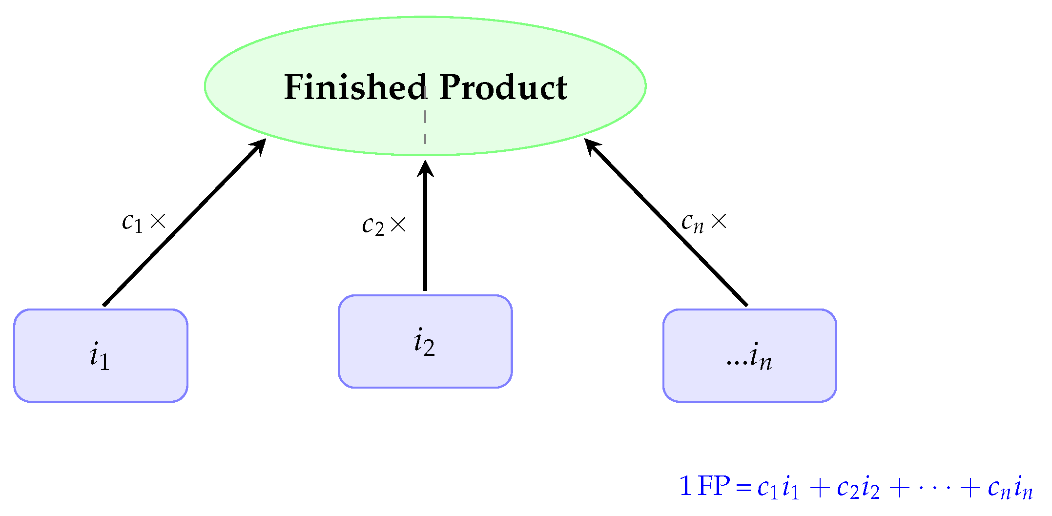
Figure 2.
Reinforcement learning process
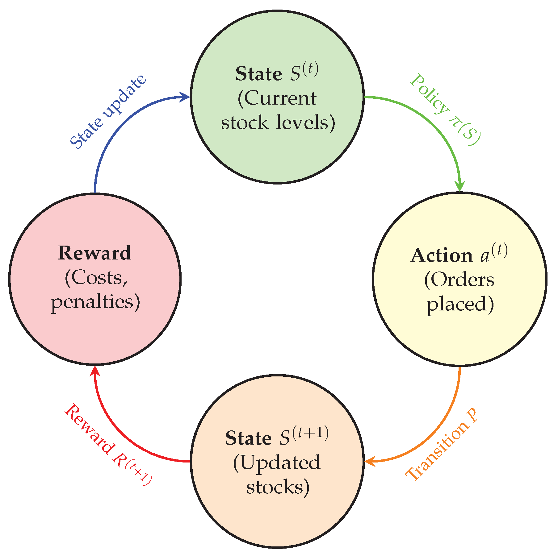
Figure 3.
Rewards per episode
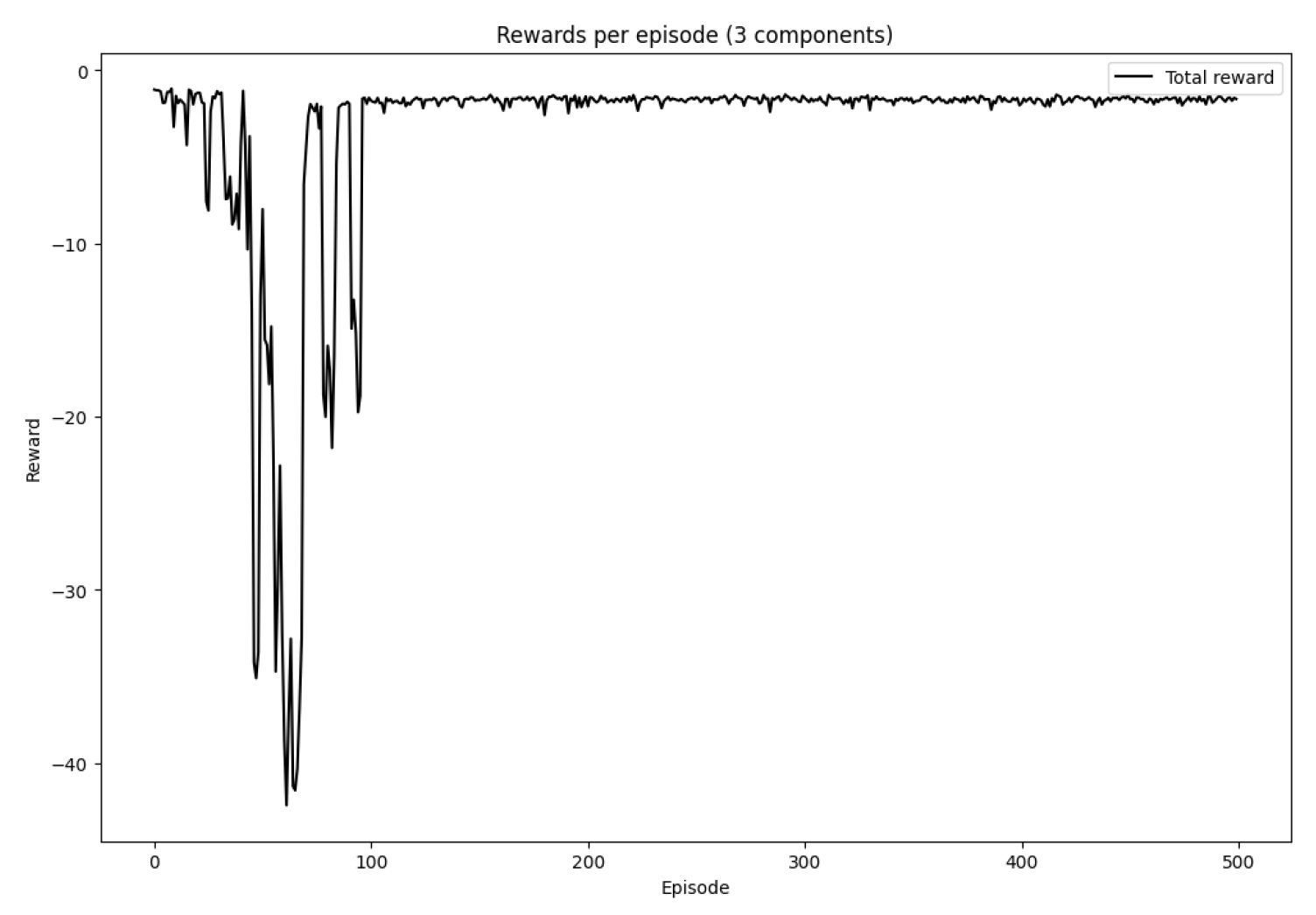
Figure 4.
Average ordering policies per episode
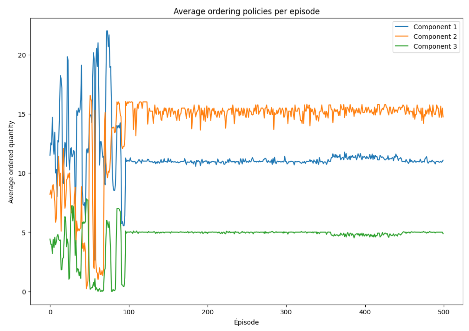
Figure 5.
Average stock levels per episode
| Criteria | Deterministic Models (EOQ, EPQ, ROP) | Stochastic Models (Q,R), (s,S), Newsvendor | Dynamic Models (Bellman, Base Stock) | Mathematical Optimization (LP, MIP) | Machine Learning (DRL) | Metaheuristic Methods |
|---|---|---|---|---|---|---|
| Approach | Assumes known demand and lead time | Uses probability distributions for demand/lead times | Multi-period optimization under uncertainty | Uses deterministic or stochastic constraints | Uses Deep RL to learn policies from data | Uses heuristic-based algorithms to explore near-optimal solutions |
| Mathematical Formulation | EOQ: EPQ: ROP: | (Q, R) Policy: Newsvendor: | Bellman Eq.: | LP/MIP: with constraints | MDP Model: | Genetic Algorithms, Simulated Annealing, Particle Swarm Optimization (PSO) |
| Handling of Demand Uncertainty | Assumes constant demand | Models demand as a random variable | Uses probabilistic demand scenarios | Models demand via stochastic constraints | Learns demand patterns dynamically | Uses probabilistic exploration |
| Handling of Lead Time Uncertainty | Assumes constant lead time | Uses safety stock: | Uses lead time as a stochastic variable | Adds lead time constraints | Learns lead time variability from data | Explores lead time variations dynamically |
| Computational Complexity | Low (closed-form solutions) | Moderate (requires statistical distributions) | High (recursive equations) | Very high (solving large models) | Very high (training models) | Moderate to High (depends on heuristics used) |
| Adaptability to Changes | Poor (recalculation needed) | Moderate (requires updated demand distributions) | High (adaptive policies) | Low (requires re-optimization) | High (continuously updates policies) | Adapts well but requires tuning |
| Optimality | Near-optimal for simple cases | Near-optimal under known distributions | Optimal in dynamic settings | Global optimality possible | Approximate optimality | Near-optimal but no guarantee of global optimum |
| Scalability | High (simple calculations) | Moderate | Low (Bellman curse of dimensionality) | Poor (high computational cost) | High (parallel learning possible) | Scales well with parallel computing |
| Implementation Complexity | Low (simple formulas) | Moderate (requires demand estimation) | High (requires recursion, DP) | Very high (formulating LP/MIP) | Very high (ML model training) | Moderate (requires careful parameter tuning) |
| Best Use Cases | Predictable demand, stable environments | Retail, periodic orders, safety stock planning | Dynamic, uncertain environments | Large-scale multi-echelon inventory | Adaptive real-time control | Large-scale, complex inventory networks |
Table 3.
Key parameters used in the simulation and learning processes.
| Category | Parameter | Value(s) | Role |
|---|---|---|---|
| Environment Parameters | num_components | 3 | Number of components in the inventory system. |
| pénalité_stock (stock penalty) | 50 | Penalty cost when the stock is zero. | |
| holding_cost | 0.5 | Storage cost per unit of stock. | |
| shortage_cost | 62 | Shortage cost per missing unit. | |
| order_cost | 1 | Ordering cost per unit ordered. | |
| initial_stock | [0, 0, 0] | Initial stock for each component. | |
| max_steps | 50 | Maximum number of steps (periods) per episode. | |
| demand_probabilities | {1: 0.2, 2: 0.5, 3: 0.3} | Probabilities of different possible demands. | |
| lead_time_probabilities | [{1: 0.3, 2: 0.5, 3: 0.2}, {1: 0.3, 2: 0.4, 3: 0.3}, {1: 0.1, 2: 0.6, 3: 0.3}] |
Probabilities of lead times for each component. | |
| consumption_coefficients | [3, 2, 1] | Consumption coefficients for each component. | |
| max_orders | Dynamically calculated based on consumption coefficients, lead times, and demand. |
Maximum quantity that can be ordered for each component. | |
| DQN Agent Parameters | state_dim | 3 (number of components) | Dimension of the state space (stock of each component). |
| action_dims | Depends on max_orders | Dimensions of the action space (quantities that can be ordered for each component). | |
| hidden_dim (neural network) | 128 | Number of neurons in the hidden layers of the neural network. | |
| lr (learning rate) | 0.30 | Learning rate for the Adam optimizer. | |
| gamma (discount factor) | 0.96 | Discount factor for future rewards. | |
| epsilon (exploration) | 1.0 (initial) | Exploration probability (choosing a random action). | |
| epsilon_min | 0.01 | Minimum value of epsilon. | |
| epsilon_decay | 0.999 | Decay rate of epsilon after each episode. | |
| batch_size | 64 | Batch size for training the neural network. | |
| num_episodes | 500 | Total number of training episodes. | |
| ReplayBuffer Parameters | capacity | 5000 | Maximum capacity of the replay buffer to store transitions. |
Table 4.
Analysis of Order Quantities and Lead Times for Each Component.
| i | Analysis |
|---|---|
|
|
|
|
|
Table 5.
Explanation of Observed Results.
| Question | Explanation |
|---|---|
| Why does have more stock than ? |
|
| Why does maintain a significant stock level despite its low consumption? |
|
| Why doesn’t have as much stock as expected (despite high consumption)? |
|
Table 8.
Factors Influencing the Optimal Ordering Policy.
| Factor | Impact on Ordering Decisions |
|---|---|
| DemandUncertainty |
|
| Lead TimeRisks | Components with longer delays need to be stocked in advance to avoid shortages. |
| CostTrade-offs |
|
| Optimal PolicyConsiderations | The optimal policy must balance these risks while considering:
|
Disclaimer/Publisher’s Note: The statements, opinions and data contained in all publications are solely those of the individual author(s) and contributor(s) and not of MDPI and/or the editor(s). MDPI and/or the editor(s) disclaim responsibility for any injury to people or property resulting from any ideas, methods, instructions or products referred to in the content. |
© 2025 by the authors. Licensee MDPI, Basel, Switzerland. This article is an open access article distributed under the terms and conditions of the Creative Commons Attribution (CC BY) license (http://creativecommons.org/licenses/by/4.0/).
Copyright: This open access article is published under a Creative Commons CC BY 4.0 license, which permit the free download, distribution, and reuse, provided that the author and preprint are cited in any reuse.


