
Submitted:
29 October 2025
Posted:
31 October 2025
You are already at the latest version
Abstract
In addressing the challenges associated with mobile robot path planning during complex product assembly measurements, this study introduces an N-step Priority Double Q Network Deep Reinforcement Learning algorithm (NDDQN). To enhance the algorithm's convergence speed, we employ double Q-learning and an N-step priority strategy during the learning phase. This approach aims to improve the obstacle avoidance capabilities of mobile robots while accelerating their learning efficiency. We conducted three grid-based obstacle avoidance simulation experiments of varying scales to compare and analyze the path planning performance of both the proximal policy optimization algorithm and the Deep Q Network algorithm. To accurately simulate real-world robotic measurement scenarios, two Gazebo environments were utilized to validate the effectiveness of our proposed algorithm. Through a comprehensive analysis of simulation results from all three algorithms, we demonstrate that the NDDQN algorithm exhibits significant effectiveness and stability in path planning. Notably, it substantially reduces iteration counts and enhances convergence speeds. This research provides a theoretical foundation for adaptive path planning in mobile robots engaged in complex product assembly measurements.
Keywords:
mobile robot
; reinforcement learning
; assembly measurement
; path planning
1. Introduction
The introduction should briefly place the study in a broad context and highlight why it is important. With the rapid advancement of Industry 4.0 technologies in the realm of intelligent manufacturing, assembly measurement path planning (AMPP) for complex products has increasingly evolved into a process characterized by digitalization, intelligence, and integrated smart control [1]. The accuracy requirements for AMPP associated with complex products are exceptionally rigorous, presenting a broad global measurement range that complicates precise positioning. Traditionally, the AMPP has predominantly relied on manual processes [2]. However, this conventional approach is characterized by relatively low efficiency. During the AMPP process, numerous measurements, including point application, calibration, and station transfer, must be executed manually [3]. This reliance on manual procedures ultimately results in extended assembly cycles and challenges in ensuring timely product delivery [4,5]. The AMPP is evolving towards a comprehensive measurement approach that integrates multiple technologies and couples various sensors. Mobile robots offer significant advantages, including substantial payload capacity and high precision in positioning accuracy [6,7]. When combined with the exceptional adaptability and flexibility of human operators, this synergy empowers robots to execute automatic assembly and measurement tasks effectively. This advancement enables flexible, high-precision assembly and measurement processes for complex products. Furthermore, the design of high-precision measurement trajectories is a crucial element in automating the assembly operations for large-scale, complex product sites, as it significantly contributes to ensuring overall assembly accuracy. Path planning for mobile robots is typically categorized into global path planning and local path planning [8]. The methods employed in global path planning primarily encompass graph search-based [9], random sampling-based [10], heuristic algorithm [11], and artificial intelligence [12]. Notably, the success of global planning methods heavily relies on the availability of prior information regarding the environment [13]. Due to the inherent uncertainty that robots encounter in complex environments, an increasing number of researchers are focusing on local path planning method. Local path planning involves the exploration of mobile robot pathways by gathering environmental information through sensors, assessing rewards and penalties, and subsequently determining the next action [14]. This process leads to the formulation of a relatively optimal collision-free path. Importantly, local path planning operates independently of prior knowledge about the environment and demonstrates excellent adaptability as well as real-time performance in response to dynamic conditions [15]. Planning algorithms encompass both obstacle avoidance planning algorithms and deep reinforcement learning [16,17]. In contrast to obstacle avoidance planning algorithms, deep reinforcement learning derives an optimal action strategy from the initial state to the target state through interactive iterative learning within the environment. As a result, deep reinforcement learning demonstrates superior adaptability to complex environments and exhibits outstanding performance in path planning for mobile robots [18].
Deep reinforcement learning (DRL), recognized as a pivotal technology in intelligent manufacturing, has garnered increasing attention from researchers regarding its application to the challenges of robot path planning [19,20]. This includes methodologies such as the Deep Q Network (DQN) algorithm, which is grounded in value functions [21], and the Deterministic Policy Gradient (DPG) algorithm [22]. Deep learning enables agents to perceive their environment, while reinforcement learning equips them with the capability to devise optimal strategies for addressing complex challenges. Consequently, deep reinforcement learning facilitates dynamic planning in uncertain environments by identifying pathways that optimize reward values to effectively reach target objectives. As a prominent deep reinforcement learning algorithm, DQN has been successfully applied across various domains, including energy management, workshop scheduling, and robotic obstacle avoidance [23]. It exhibits considerable efficacy in addressing path planning challenges within uncertain environments. Smart et al [24] were pioneers in applying Q-learning to the problem of robot navigation, developing a straightforward reward function to assist robots in identifying viable solutions. Low et al [25] introduced an enhanced DQN designed to tackle path planning challenges, thereby improving the convergence speed of Q-learning. However, this approach encounters difficulties in effectively adapting to complex working environments during the path planning process. Cheng et al [26] proposed a streamlined deep reinforcement learning algorithm for obstacle avoidance, leveraging a robust DQN architecture that effectively addresses both obstacle avoidance and path planning challenges faced by unmanned vessels. Lou et al [27] advanced a method that integrates DQN with prior knowledge through the design of a fuzzy logic controller, which significantly aids robots in mitigating unproductive exploration and consequently reduces training time. To solve the sequential decision-making problem of ship collision avoidance, Yang et al [28] improved DQN by sampling priority and adopting non-uniform sampling techniques, subsequently validating their proposed algorithm within a simulation environment. Nakamura et al [29] utilized DQN to obtain the control strategy for path planning on narrow roads, facilitating the robot's ability to reach its target with minimal speed variations and fewer turns in constrained environments. To achieve collection-free path planning in complex environments, Gu et al [30] applied M-DQN to address the mobile robots' path planning challenges. By decomposing the network architecture and incorporating an artificial potential field as a reward function, they attained an enhanced learning strategy. Hu et al [31] proposed a multi-agent deep deterministic policy gradient method to solve the anti-collision problem of AGVs in container terminal transportation, utilizing the Gumbel-softmax technique to discretize scenarios generated by the node network. Li et al [32] proposed a deep learning algorithm combining Angle search and DQN to achieve precise control over the search direction of mobile robots, thereby enhancing the efficiency of path planning. Wu et al [33] proposed a path planning method for multi-robot systems based on distributed multi-agent deep reinforcement learning, allowing for local optimal path planning that take into account the behaviors of other robots. To address issues related to low solution efficiency and blind exploration in robot path planning, Li et al [34] proposed an adaptive Q-learning algorithm based on virtual target guidance. This method incorporates a dual memory mechanism and an adaptive greed factor, effectively improving the convergence speed of the algorithm.
To enable robots to make adaptive decisions in complex environments, DRL brings new potential to robot path planning. Hua et al [35] present an advanced hierarchical motion planning strategy that synergistically combines DRL with collaborative design of motion optimization, aiming to achieve efficient and seamless navigation in unfamiliar environments. Zhao et al [36] introduced an advanced hierarchical path planning framework that intricately integrates global path planning with local dynamic obstacle avoidance, leveraging the power of deep reinforcement learning alongside the Grey Wolf optimization algorithm. This innovative approach aims to facilitate efficient and secure navigation for robots operating within unpredictable environments. Dawood et al [37] employed multi-agent reinforcement learning (MARL) to address the intricacies of behavior-based cooperative navigation for mobile robots, successfully achieving a paradigm of safe and efficient collaborative movement. Jonnarth et al [38] explored the potential of continuous spatial reinforcement learning in the realm of coverage path planning, empowering agents to adeptly adapt to distinct environmental characteristics. Jiao et al [39] introduced a deep reinforcement learning algorithm featuring automatic entropy adjustment tailored for shearing, aimed at enhancing the efficacy of strategy acquisition in mobile robots by effectively mitigating the evaluation of entropy.
DRL algorithms have achieved remarkable advancements in the realm of path planning, but it still harbors certain shortcomings. The intricacies of reward mechanism design are significantly reliant on expert prior knowledge and necessitate a delicate balance among various objective criteria, including path length, safety considerations, and energy efficiency [40,41]. Furthermore, the opaque nature of the DRL algorithm engenders a lack of interpretability in its decision-making processes, rendering it challenging to furnish formal guarantees regarding security [42]. Throughout the training process, the convergence performance remains unstable, and the agent is prone to collisions with obstacles. When the next action taken by the agent relies solely on observed environmental data, the DRL path planning algorithm demonstrates insufficient generalization capabilities [43]. To address these issues regarding slow convergence rates and inadequate generalization capabilities in DRL, we introduce N-step priority strategy and double Q-learning techniques. This work aims to propose an N-step priority double DQN learning algorithm (NDDQN), wherein the learning strategy leverages not only the current state of the agent but also its target location. By selecting appropriate actions grounded in this comprehensive understanding, we guide the robot in its pursuit of optimal path.
In comparison with the existing studies, this paper makes the following contributions:
A NDDQN algorithm with N-step priority experience replay and double-Q learning is proposed. This method effectively addresses the challenges of sluggish convergence and the overestimation bias commonly encountered in DRL for mobile robot path planning. By mitigating maximum operational deviations through a double DQN, expediting the acquisition of experiences via prioritized sampling, and employing N-step updates to adeptly rewards forward, this method ensures not only an accelerated convergence rate but also enhanced stability in the learning process.
We have adeptly refined the reward function and experience replay strategy, significantly alleviating the challenge of sluggish learning rates encountered in DRL algorithms. The estimation of rewards is conducted utilizing the double DQN, which proficiently mitigates overestimation issues and enhances both the accuracy and stability of Q value estimations. Moreover, prioritized experience replay amplifies the weight priority assigned to stored experiences, thereby facilitating a more efficient exploitation of data resources.
We meticulously crafted an abstract discrete grid environment alongside a highly sophisticated continuous dynamic simulation framework to address the challenges posed by mobile robot model adaptation in both dynamic and static settings. Our approach has facilitated remarkably efficient adaptive path planning for mobile robots, which has been rigorously validated with respect to its generalization capabilities and robustness.
The rest of this paper is organised as follows: Section 2 is problem description and modeling. Section 3 introduces the improved deep reinforcement learning algorithm. Section 4 presents the experimental verification and analysis. Section 5 summarizes the content of the study and outlines areas for future research.
2. Problem Description and Modeling
2.1. Problem Description
The assembly measurement process for complex products is conducted by a mobile measurement robot equipped with a scanner, which automatically scans the workpiece along a predetermined trajectory. Taking the assembly measurement process of an aircraft tube section as an example, the simplified schematic model is illustrated in Figure 1. The measurement robot utilizes the scanner to perform localized scanning operations, ensuring that the scanning path runs parallel to the axis of the large-diameter cylindrical product. Upon completing the scanning process for one measuring unit and transitioning to the next, the robot executes a horizontal movement to facilitate this transfer operation.
The measurement task encompasses five distinct measurement units: S1 and S2 are conical surfaces, while S3 is a cylindrical surface. Additionally, S4 and S5 consist of symmetrically arranged circular planes. The measurement area encompasses overlapping regions that enhance image stitching capabilities, thereby improving overall scanning accuracy. The measurement robot conducts shape scanning of each component along a predetermined trajectory path and subsequently acquires point cloud data. The measurement robot and the calibration target are positioned within the visible range of the tracker, which plans its movement trajectory based on an optimized scanning path. The primary function of the tracker is to ascertain the spatial position of the measuring robot, thereby facilitating an indirect determination of the scanner's spatial position. Scanning data is subsequently transferred into a global coordinate system via the laser tracker's measurement coordinate system, effectively achieving unification within the spatial measurement domain. The object under examination undergoes a comprehensive scanning process. It is crucial for the tracker to maintain proximity to this object in order to ensure precise measurements.
2.2. Dynamic Modeling for Mobile Robots
The mobile measurement robot is primarily utilized for the precise scanning of assembly dimensions in AMPP. This system comprises omnidirectional mobile automated guided vehicles (AGVs), industrial robotic arms, distance sensors, visual guidance systems, and end support devices. Equipped with five ultrasonic distance sensors, the mobile measurement robot can effectively determine its directional orientation. The angle between each direction measured by these ultrasonic sensors is set at 45 degrees. The kinematic structure of the robot, along with its integrated sensors, is depicted in Figure 2. In this illustration, XOY represents the global coordinate system, while X'OY' denotes the local coordinate system of the robot. The term refers to the distance between the left and right wheels. When a robot performs a turn, the point around which it rotates is referred to as the instantaneous curvature center . represents the angle between the center of the robot and the global coordinate system. The position of the robot can be expressed using global coordinates and its directional orientation.
The mobile robot's movement is facilitated through a differential drive system. Consider that the left front wheel and the left rear wheel of the robot operate at an identical linear velocity, denoted as , while the right front wheel and the right rear wheel maintain a consistent linear velocity represented as . The forward linear velocity and the turning angular velocity of the robot are as shown in Formula (1).
When the robot turns, the instantaneous curvature radius between the robot center and the curvature center is calculated as Formula (2):
Generally, the motion data directly read by mobile robots is based on the local coordinate system. The motion data in the global coordinate system is obtained through Euler transformation, and the formula is using Formula (3).
In light of the premise of uniform motion, the trajectory generation and assessment for the mobile robot will be directly derived from the sequence of actions undertaken, thereby obviating the need for explicit integration of left and right wheel velocities in computational processes. This comprehensive model is meticulously crafted to furnish a robust theoretical foundation for evaluative indicators while simultaneously establishing interfaces that anticipate future investigative endeavors.
3. Improved Deep Reinforcement Learning Algorithm
The path planning model for the mobile robot presented above constitutes a complex nonlinear optimization problem. The uncertainty associated with the number of inflection points in the robot's trajectory introduces variability in the resultant path. Deep reinforcement learning algorithms facilitate path optimization for mobile robots operating within uncertain environments by leveraging neural network learning capabilities. Consequently, this study addresses the path planning model relevant to robotic assembly measurement through enhancements in deep learning algorithms.
Figure 3 illustrates the framework predicated on the NDDQN algorithm. We have devised a path planning model for mobile robots utilizing NDDQN, framing the path planning conundrum as a Markov decision process. Subsequently, the mobile robot acquires environmental data through an array of sensors and meticulously calculates both the direction and distance to obstacles as well as target objects. The mobile robot selects action values from the replay buffer by employing prioritized experience replay while simultaneously referencing the reward function. These action values and states are then processed through layers of neural networks, culminating in the output of Q values aimed at minimizing loss functions, which are subsequently fed back into the neural network for parameter updates. Upon reaching its designated endpoint, it assesses whether convergence has been achieved. If convergence is confirmed, the program concludes; otherwise, it persists in generating new target endpoints and engaging with its environment until termination occurs. Ultimately, this interaction enables the mobile robot to gather training data and refine its learning based on sampled information.
3.1. Markov Process
The path planning problem for mobile robot installation and testing can be regarded as a Markov process. In each time step, the robot agent will choose an action to change the environmental state, which is represented as a five-tuple . The environment returns the next state and reward of the robot agent, and the robot agent selects the next action based on the reward. Under the time step , the state of the environment is , the agent selects action , and the environment provides the next state , the next reward and the discount factor , where the discount factor is used for the discount reward, and . The set of all states is the state space , and the set of all actions is the action space . The probability distribution of each state behavior is strategy . The robot agent selects action through strategy , and represents the probability of choosing action in state . The transfer function represents the probability of obtaining the next state under state and behavior , and represents the reward for choosing behavior under state , as Formula (4).
The cumulative rewards of the robot agent are as follows.
where the discount factor of step k is , and the goal of reinforcement learning is to maximize the cumulative reward .
The value estimation of reinforcement learning is defined as a value function, which is divided into state value functions and action value functions. The state value function represents the expected reward of the strategy in the state, and the action value function represents the expected reward of the strategy taking actions in the state, as shown in Formulas (6) and (7).
The relationship between and can be expressed as . The optimal strategy selects the action with the maximum action value for each state , as shown in Formula (8).
The optimal state value and the optimal action value can be calculated as
Therefore, the goal of reinforcement learning can be transformed into solving the optimal state value and action value .
3.2. Double-Q Learning
When the state space or action space is excessively large, accurately estimating the value of each action becomes a challenging task. Consequently, the incorporation of deep neural networks to approximate the action value function has given rise to what is known as deep reinforcement learning. In the context of deep Q-networks, the optimization objective is to progressively minimize the discrepancy between the estimated return value and the predicted action value. This involves updating network weight through loss function optimization, as illustrated in Formula (11).
In the process of enhancing DQN, the introduction of a target network serves to improve stability. In DQN's update mechanism, the neural network utilized for estimating rewards is identical to that used for action value estimation. Consequently, it leads to fluctuations in the estimated values as parameters vary. The updating of DQN's action values can easily result in an overestimation bias. To address this issue of overestimation, Double Q-learning employs a strategy where actions are selected using the evaluation network while utilizing the target network for reward estimation. Accordingly, the loss function is represented as shown in Formula (12).
where is the target network.
3.3. Priority Experience Reply
Experience replay serves as a storage mechanism that retains actions, behaviors, and rewards within a discrete time step. During the training process, samples are drawn from the stored experiences based on specific criteria, after which the network is updated utilizing these sampled experiences. This paper employs prioritized experience replay (PER) to enhance the weight priority of the stored experiences. In DQN, the temporal difference (TD) error represents the discrepancy between the target value and the current value. A larger TD error significantly influences backpropagation. Conversely, a smaller TD error results in reduced influence of that sample on gradient descent updates. Refining this concept further, prioritized experience replay can expedite the convergence speed of the network. This work introduces SumTree to store samples in priority experience replay [44]. All empirical samples are stored at the bottom leaf nodes, where the leaf nodes preserve the sample priorities. The top of the SumTree is the sum of the experiences of all samples. Then, the loss function of the sample priorities becomes formula (13).
where is the priority weight of the jth sample. After performing gradient update on the Q network, the TD error needs to be recalculated and the SumTree updated.
3.4. Priority N-step Update Strategy
The above-mentioned method is a one-step update method, which only uses the information of the current time step and the next time step, that is
To accelerate the learning process, an N-step update strategy is adopted and multi-step information is used for updates. The return value of step N is expressed as
Then, the loss function is as formula (16).
By adopting the above-mentioned NDDQN algorithm, taking the current position, movement information and current speed of the mobile robot as the input states, the movement direction of the mobile robot is regulated by this algorithm.
4. Experimental Verification and Analysis
4.1. Exoerimental Environment
To verify the effectiveness of the proposed NDDQN algorithm, comparative experiments were conducted in two training environments, namely the virtual Grid Map environment and the Gazebo simulation environment. The Grid Map experiment builds a GUI environment model on the built-in standard library of PyCharm. The experiment adopted a 1m×1m grid map, where black squares represent obstacles, blank areas are passable zones, the lower left corner is the starting point, the upper right corner is the target point, and the black lines throughout the map represent the grid. The developed grid environments are 10×10, 20×20 and 30×30 respectively. The robot agent is located on the map by the coordinates of the two diagonal points.
The Gazebo simulation environment similar to the real-world environment is: an environment with static obstacles (E1); An environment containing both static and dynamic obstacles (E2). The Gazebo robot serves as a mobile measurement platform for testing in a simulated environment. The environment E1 has 13 fixed rectangular obstacles, with white objects serving as static obstacles. The layout of environment E2 is more complex. Two blue cylinders are randomly placed in the environment as moving obstacles. Six target points (P1 to P6) are placed in the unobstructed area within the environment.
The total number of training rounds of the simulation experiment is set to 1000 episodes. When the agent reaches the target or collides, the current round terminates. The training is completed when the total reward of the agent reaches a stable and satisfactory level. The computer environment is 2.1GHz Intel Core i7-12700, 128GB of memory, and the operating system is windows11. Various path planning algorithms are implemented using Python 3.12 and invoke the built-in interfaces. TensorFlow is used to define neural network architectures, enabling models to gain GPU-accelerated advantages during the training process. In all the simulation experiments, the same robot model parameters were set. The mobile robot is trained by different algorithms, and then experiments are conducted using the empirical dataset generated from the training to verify the performance of the proposed algorithms. Table 1 presents the network hyperparameters of the NDDQN algorithm, detailing both network and training parameters. The fully connected layers of the network are managed substantial amounts of data, with the first layer containing 256 units, the second with 256 units, and the third with 128 units. This study employs a maximum epoch limit of 1000 across all training algorithms and establishes a maximum exploration step threshold of 800 for continuous learning as well as algorithm feasibility evaluation. The mobile robot learning rate is fixed at 0.005. To facilitate efficient training and enhance the learning rate of the NDDQN algorithm, we set the minimum batch learning size to 64 and the discount factor to 0.95. The proposed algorithm network updates occur at a 0.001 update rate between the current and target networks. The optimal distance that a mobile robot should maintain while in motion is set at 0.5 meters. Comparative simulation experiments were conducted respectively for the NDDQN algorithm, the proximal policy optimization (PPO) algorithm [45] and the DQN algorithm [24] in different scenarios, and the convergence was analyzed.
4.2. Deep Learning Parameter Settings
The settings of deep reinforcement learning include states, goals, behaviors and reward functions. The status is determined by the information obtained by the ultrasonic sensor. The target includes the distance from the current position of the robot to the target point, as well as the relative direction of the target point relative to the robot. The calculation formula is as follows.
where and are the coordinates of the robot and the target point relative to the global coordinate system.
For the behavior of mobile robots, it is manifested as five actions: forward movement, left turn, right turn, quick left turn and quick right turn. The forward linear velocity and the turning angular velocity corresponding to the action are shown in Table 2. Each action lasts for 1 second. After the agent completes the current action, it will re-read the status and target information and proceed to the next action.
When setting the reward function, the reward depends on the distance of the obstacle, the collision with the obstacle, and the comprehensive score of reaching the target point. The reward function includes a negative reward for collision, a reward for reaching the target point, and a positive reward for maintaining a safe distance. To prevent the agent from colliding with the surrounding environment during movement, when the robot agent collides, it will receive a negative reward of . To encourage agents to move towards the target point, the closer the agent is to the target, the higher the reward will be. When the agent successfully reaches the target position, a positive reward of will be directly given. When the agent approaches the collision obstacle, the states of the robot agent are divided into the safe distance state and the non-safe distance state . To reduce the possibility of colliding with obstacles, the definition of the safety distance reward is as follows.
Therefore, when the agent reaches the target point, the comprehensive reward function is as formula (20).
4.3. Simulation Results Analysis in Grid Map
To verify the effectiveness of the proposed NDDQN algorithm in solving the path planning problem, simulation experiments were conducted using grid obstacles of different scales to verify the effectiveness of the proposed algorithm in solving the path planning problem. To achieve the simulation scenarios of small-scale, medium-scale and large-scale examples, grid simulation examples of three scenarios, namely 10×10, 20×20 and 30×30, are constructed. In this paper, four parameters, namely the total substitution value of the path, the maximum completion time, the total length of the path and the total number of turns of the path, are adopted as the evaluation indicators for solving the quality of the path. After 800 generations of training, the convergence of the models trained by NDDQN, DQN and PPO was compared. The comparison of the average rewards of the three algorithms is shown in Figure 4, Figure 5 and Figure 6. In small-scale simulation examples, the convergence speeds of the three algorithms do not differ much and basically achieve convergence after 100 generations of training. In the medium-scale simulation results, NDDQN has a relatively fast convergence speed and a high reward value. The three algorithms reach convergence around the 130th generation. In the large-scale simulation results, the iteration speed of NDDQN is significantly accelerated. It can avoid obstacles and reach the target point more quickly, and the number of training generations required to reach the target is smaller than that of the other two algorithms. With the increase of environmental complexity, the number of convergence generations required by the agent has a continuous increasing trend, and the final reward value is also increasing.
To compare the stability of the models trained by the three methods, 50 tests were conducted on the trained models under the same conditions. The average results are shown in Table 3. It can be seen from the training results of the three scenarios that the arrival time, total path length, turning times and average curvature of NDDQN are significantly lower than those of the other two algorithms, and the total reward values are all higher than those of DQN and PPO algorithms. The powerful learning ability of NDDQN is more prominent in complex scenarios, reaching the destination with the fewest turns and the highest reward value. The paths selected by the three algorithms when successfully reaching the target point are shown in Figure 7, Figure 8 and Figure 9. Among them, the blue line represents the NDDQN planning path, the yellow line represents the DQN planning path, and the red line represents the PPO planning path. It can be seen from the simulation paths that the paths for NDDQN and DQN to reach the target point are similar, and the number of turns required to reach the target is relatively small. Although the path planned by the DQN algorithm is similar to that of the NDDQN algorithm, the path length is longer, so the time is longer. The path planning obstacle avoidance ability of the PPO algorithm is more prominent. However, during the exploration process, there are more turns, resulting in a larger total path length and an increase in the time to reach the destination accordingly. To sum up, the experimental simulation results demonstrate the effectiveness of the NDDQN algorithm, which can help mobile robots obtain more effective obstacle avoidance experience in the task of measurement path planning.
4.4. Simulation Results Analysis in Gazebo
In the E1 and E2 test environments, there are six selected navigation points (P) and two moving obstacle points (D). The robot's task is to independently explore the environment, traverse from position P1 to P6, and then return to the initial position S without colliding with obstacles. To verify the effectiveness of the proposed NDDQN algorithm, we conducted path planning simulations in two Gazebo simulation environments. In scenario E1, the robot achieved path exploration from position P1 to P6 and returned to the target position S, as shown in Figure 10. In scenario E2, the robot completed the path exploration from position P1 to P6, avoided two dynamic obstacles, and successfully returned to the target position S, as shown in Figure 11.
In the static environment, the robot meticulously devises a smooth and nearly optimal trajectory from S to P6 and back, exemplifying the algorithm's remarkable efficiency in navigating obstacle-free pathways. As illustrated in Figure 10, the robot's trajectory is direct and streamlined, epitomizing a goal-oriented path characterized by minimal redundancy. In stark contrast, the dynamic environment presents two mobile obstacles, as depicted in Figure 11. The generated path clearly reveals noticeable detours and recalibration points where the robot adeptly anticipated and circumvented collisions prior to advancing towards its target and returning to S. These detours are far from arbitrary. They represent strategic avoidance maneuvers executed with precision to uphold a safe distance from the projected trajectories of dynamic obstacles. This vividly underscores the algorithm's robustness and real-time responsiveness when confronted with dynamic impediments. The comparative analysis conclusively demonstrates that while the algorithm excels at identifying optimal paths within static contexts, its paramount strength lies in its predictive avoidance capabilities amidst dynamic scenarios.
The ability of the cumulative reward response algorithm path planning for robot agents. To more intuitively reflect the characteristics of each agent reward, Figure 12, Figure 13 and Figure 14 present the total rewards of the three algorithms in the E1 environment. As shown in Figure 14, the NDDQN algorithm is significantly superior to other algorithms. The reward converging to 2600 is significantly higher than 1000 for PPO and 1700 for DQN. Similarly, in the more complex E2 environment, the performance gap is even greater. The superior performance of NDDQN in both environments proves that it can learn the optimal strategy more effectively. The simplicity of PPO limits its performance. Although DQN performs well, it is still surpassed by the efficient learning ability of NDDQN.
Table 4 compares the success rates and convergence times of the PPO, DQN, and NDDQN algorithms used for path planning in two scenarios. For the E1 scenario, the success rate of the NDDQN algorithm is 34.4% higher than that of the DQN algorithm and 58.5% higher than that of PPO. Table 4 simultaneously compares the convergence speeds of the three algorithms. The shortest time required for NDDQN to obtain the final target point is 114 minutes, while PPO and DQN take 248 and 153 minutes respectively. For the E2 scenario, the introduction of dynamic obstacles leads to a decline in the performance of all algorithms. The success rate of NDDQN was 60.2% and 39.4% higher than that of PPO and DQN, respectively. NDDQN converges the fastest and completes the path task in 142 minutes. This performance outperforms the DQN algorithm, which takes 193 minutes to converge, and is faster than PPO, which takes 286 minutes. These simulation results prove that NDDQN performs superior in both dynamic and static environments, demonstrating a faster convergence speed and learning efficiency.
4.5. Ablation Study
To validate the efficacy of each integrated strategy employed in this study and its contribution to overall performance, we conducted a series of ablation experiments focusing on double Q-learning (DQL), priority experience replay (PER), and N-step returns. The objective of these experiments is to quantitatively assess the impact of omitting any given strategy on the algorithm's performance, thereby elucidating its essentiality. The experimentation was carried out within the Gazebo environment, allowing us to compare five distinct configurations: 1) Our model: NDDQN; 2) -N-step: excluding n-step returns while relying solely on single-step TD errors; 3) -PER: eliminating PER in favor of uniform random sampling; 4) -DQL: removing DQL to revert to the target value computation method utilized by traditional DQN; and 5) Benchmark DQN: employing the standard DQN algorithm as a baseline for performance comparison. All models were configured with an identical set of hyperparameters, ensuring consistency across tests. Each configuration underwent independent execution for ten iterations to garner statistically significant results. In assessing asymptotic performance, we elected to utilize average final returns. Sample efficiency and learning speed were measured by the number of training steps required to achieve predetermined performance thresholds. Finally, stability and robustness were quantified through evaluating the standard deviation across multiple return runs.
The experimental results are shown in Table 5. All strategies are key contributors to the overall performance of the proposed algorithm, but their main aspects of influence are different. The N-step model has the most significant damage to the convergence speed of the algorithm. The number of training steps required to reach the threshold is approximately 45% higher than that of the NDDQN model, indicating that the multi-step reward mechanism plays a core role in accelerating temporal credit allocation and policy optimization. The -PER shows the most severe degradation in terms of final performance and stability, with the lowest average return and the largest standard deviation. This highlights the irreplaceability of PER in enhancing sample efficiency and avoiding training stagnation by prioritizing the replay of high-learning-value experiences. Although -DQL can achieve a final performance close to that of NDDQN model, its stability significantly decreases, verifying the crucial role of -DQL in alleviating Q value overestimation and ensuring smooth convergence in the learning process. Ultimately, the NDDQN model significantly outperformed all ablation variants and benchmark models in all evaluation dimensions. This not only demonstrated the effectiveness of each component but also indicated a positive synergy among them, collectively forming an efficient, stable, and robust reinforcement learning agent.
5. Conclusions
This study introduces a path planning algorithm founded on deep reinforcement learning, specifically designed to address the complexities associated with mobile robot assembly and measurement path planning within the intricate processes of aerospace product assembly and measurement. Firstly, the path planning problem pertaining to the installation and testing phases of the mobile robot is defined through model simplification, followed by dynamic modeling of the mobile robot. Secondly, to enhance the convergence speed of deep learning algorithms, Double DQN is employed for evaluating network selection actions. The implementation of reward estimation using a target network effectively mitigates issues related to overestimation. To further expedite network convergence, SumTree is introduced for storing samples within prioritized experience replay. Additionally, an N-step update strategy is incorporated to strengthen the robot's obstacle avoidance capabilities of the robot while enhancing its learning rate by updating using multi-step information. Finally, grid-based obstacle avoidance simulation experiments are conducted across three grid map environments, 10×10, 20×20, and 30×30. These experiments aim to compare and analyze the path planning performance of various algorithms. We conducted simulations of robot path planning capabilities under the influence of both static and dynamic obstacles within the Gazebo simulation environment. The results indicate that, compared to others path planning algorithms, the proposed NDDQN algorithm exhibits superior solution efficiency and stability in path planning tasks. Importantly, its path optimization capability becomes particularly pronounced in complex environments. Future research will focus on tackling complex path planning problems involving multiple robots and numerous target points while analyzing the generalization capability of robotic collision avoidance against diverse types of obstacles to further enhance adaptive path planning abilities. To ultimately realize the goal of deployment, future endeavors must encompass the meticulous performance profiling of representative robotic computing platforms. Furthermore, it is imperative to devise innovative optimization strategies aimed at mitigating computational costs.
Author Contributions
Conceptualization, G.Y. and B.Z.; methodology, G.Y. and B.Z.; software, G.Y.; validation, B.Z., Y.H. and G.T.; formal analysis, G.Y.; investigation, B.Z.; resources, Y.H.; data curation, B.Z.; writing—original draft preparation, G.Y.; writing—review and editing, Z.L.; visualization, G.T.; supervision, Z.L.; project administration, G.Y.; funding acquisition, G.Y. All authors have read and agreed to the published version of the manuscript.
Funding
This research received funding within the National Natural Science Foundation of China under Grant No.52405537, Humanities and Social Science Fund of Ministry of Education of China under Grant No.24YJCZH446, the National key Research and Development Program of China under Grant No. 2023YFE0198600, and the Jiangsu Excellent Postdoctoral Program under Grant No. 2023ZB634.
Informed Consent Statement
Informed consent was obtained from all subjects involved in the study.
Data Availability Statement
Data can be obtained by contacting the corresponding author.
Conflicts of Interest
The authors declare no conflicts of interest.
Abbreviations
The following abbreviations are used in this manuscript:
| The robot's position of the global coordinate. | |
| The target point's position of the global coordinate. | |
| The linear velocity of the left front wheel and the left rear wheel of the robot. | |
| The linear velocity of the right front wheel and the right rear wheel. | |
| The forward linear velocity of the robot. | |
| The turning angular velocity of the robot. | |
| The instantaneous curvature center. | |
| The instantaneous radius of curvature. | |
| The Angle between the center of the robot and the global coordinate system. | |
| The reward of the robot agent. | |
| The state of robot agent. | |
| The action of the robot agent. | |
| The next state of robot agent. | |
| The next action of the robot agent. | |
| The next reward of the robot agent. | |
| The discount factor, and . | |
| The state space of robot. | |
| The action space of robot. | |
| The strategy of each state behavior. | |
| The probability of choosing action in state . | |
| The probability of obtaining the next state under state and behavior | |
| The reward for choosing behavior under state | |
| The cumulative reward of robot agent. | |
| The optimal strategy of robot agent. | |
| The optimal state value of robot agent. | |
| The optimal action value of robot agent. | |
| The updating network weight. | |
| The loss function. | |
| The target network. | |
| The priority weight of the jth sample. | |
| α | Learning rate. |
References
- Chen, Z.; Li, T.; Jiang, Y. Image-Based Visual Servoing With Collision-Free Path Planning for Monocular Vision-Guided Assembly. IEEE Trans. Instrum. Meas. 2024, 73, 1–17. [CrossRef]
- Monaco, E.; Rautela, M.; Gopalakrishnan, S.; Ricci, F. Machine learning algorithms for delaminations detection on composites panels by wave propagation signals analysis: Review, experiences and results. Prog. Aerosp. Sci. 2024, 146. [CrossRef]
- Ali, M.; Das, S.; Townley, S. Robot Differential Drive Navigation Through Probabilistic Roadmap and Pure Pursuit. IEEE Access 2025, 13, 22118–22132. [CrossRef]
- Zhao, M.; Zhang, Q.; Zhao, T.; Tian, H. Research on Reducing Assembly Errors in Inductive Encoders With Observer Phase Detector Phase-Locked Loop. IEEE Sensors J. 2023, 23, 28744–28751. [CrossRef]
- SUI, S.; ZHU, X. Digital measurement technique for evaluating aircraft final assembly quality. Sci. Sin. Technol. 2020, 50, 1449–1460. [CrossRef]
- Unhelkar, V.V.; Dorr, S.; Bubeck, A.; Lasota, P.A.; Perez, J.; Siu, H.C.; Boerkoel, J.C.; Tyroller, Q.; Bix, J.; Bartscher, S.; et al. Mobile Robots for Moving-Floor Assembly Lines: Design, Evaluation, and Deployment. IEEE Robot. Autom. Mag. 2018, 25, 72–81. [CrossRef]
- Yuan, G.; Lv, F.; Shi, J.; Tian, G.; Feng, Y.; Li, Z.; Pham, D.T. Integrated optimisation of human-robot collaborative disassembly planning and adaptive evaluation driven by a digital twin. Int. J. Prod. Res. 2024, 1–19. [CrossRef]
- Xiang, Y.; Jin, X.; Lei, K.; Zhang, Q. Research on Energy-Saving and Efficiency-Improving Optimization of a Four-Way Shuttle-Based Dense Three-Dimensional Warehouse System Based on Two-Stage Deep Reinforcement Learning. Appl. Sci. 2025, 15, 11367. [CrossRef]
- Liu, Q.; Wang, C. A graph-based pipe routing algorithm in aero-engine rotational space. J. Intell. Manuf. 2013, 26, 1077–1083. [CrossRef]
- Ni, J.; Ge, Y.; Zhao, Y.; Gu, Y. An Improved Multi-UAV Area Coverage Path Planning Approach Based on Deep Q-Networks. Appl. Sci. 2025, 15, 11211. [CrossRef]
- Chi, W.; Ding, Z.; Wang, J.; Chen, G.; Sun, L. A Generalized Voronoi Diagram-Based Efficient Heuristic Path Planning Method for RRTs in Mobile Robots. IEEE Trans. Ind. Electron. 2021, 69, 4926–4937. [CrossRef]
- Tong, X.; Yu, S.; Liu, G.; Niu, X.; Xia, C.; Chen, J.; Yang, Z.; Sun, Y. A hybrid formation path planning based on A* and multi-target improved artificial potential field algorithm in the 2D random environments. Adv. Eng. Informatics 2022, 54. [CrossRef]
- Qin, J.; Qin, J.; Qiu, J.; Liu, Q.; Li, M.; Ma, Q. SRL-ORCA: A Socially Aware Multi-Agent Mapless Navigation Algorithm in Complex Dynamic Scenes. IEEE Robot. Autom. Lett. 2023, 9, 143–150. [CrossRef]
- Soualhi, T.; Crombez, N.; Ruichek, Y.; Lombard, A.; Galland, S. Learning Decentralized Multi-Robot PointGoal Navigation. IEEE Robot. Autom. Lett. 2025, 10, 4117–4124. [CrossRef]
- Guralnik, D.P.; Stiller, P.F.; Zegers, F.M.; Dixon, W.E. Plug-and-Play Cooperative Navigation: From Single-Agent Navigation Fields to Graph- Maintaining Distributed MAS Controllers. IEEE Trans. Autom. Control. 2023, 69, 5262–5277. [CrossRef]
- Lee, C.-C.; Song, K.-T. Path Re-Planning Design of a Cobot in a Dynamic Environment Based on Current Obstacle Configuration. IEEE Robot. Autom. Lett. 2023, 8, 1183–1190. [CrossRef]
- Liu, S.; Shi, Z.; Lin, J.; Yu, H. A generalisable tool path planning strategy for free-form sheet metal stamping through deep reinforcement and supervised learning. J. Intell. Manuf. 2024, 36, 2601–2627. [CrossRef]
- Xue, Y.; Chen, W. RLoPlanner: Combining Learning and Motion Planner for UAV Safe Navigation in Cluttered Unknown Environments. IEEE Trans. Veh. Technol. 2023, 73, 4904–4917. [CrossRef]
- Bai, Z.; Pang, H.; He, Z.; Zhao, B.; Wang, T. Path Planning of Autonomous Mobile Robot in Comprehensive Unknown Environment Using Deep Reinforcement Learning. IEEE Internet Things J. 2024, 11, 22153–22166. [CrossRef]
- Ding, X.; Chen, H.; Wang, Y.; Wei, D.; Fu, K.; Liu, L.; Gao, B.; Liu, Q.; Huang, J. Efficient Target Assignment via Binarized SHP Path Planning and Plasticity-Aware RL in Urban Adversarial Scenarios. Appl. Sci. 2025, 15, 9630. [CrossRef]
- Ejaz, M.M.; Tang, T.B.; Lu, C.-K. Vision-Based Autonomous Navigation Approach for a Tracked Robot Using Deep Reinforcement Learning. IEEE Sensors J. 2020, 21, 2230–2240. [CrossRef]
- Zhou, C.; Huang, B.; Fränti, P. A review of motion planning algorithms for intelligent robots. J. Intell. Manuf. 2021, 33, 387–424. [CrossRef]
- Zhang, L.; Zhang, Y.; Li, Y. Mobile Robot Path Planning Based on Improved Localized Particle Swarm Optimization. IEEE Sensors J. 2020, 21, 6962–6972. [CrossRef]
- W.D. Smart; L.P. Kaelbling. Effective reinforcement learning for mobile robots. Proceedings 2002 IEEE International Conference on Robotics and Automation 2002, Volume 4, 3404–3410.
- Low, E.S.; Ong, P.; Cheah, K.C. Solving the optimal path planning of a mobile robot using improved Q-learning. Robot. Auton. Syst. 2019, 115, 143–161. [CrossRef]
- Cheng, Y.; Zhang, W. Concise deep reinforcement learning obstacle avoidance for underactuated unmanned marine vessels. Neurocomputing 2018, 272, 63–73. [CrossRef]
- Lou, P.; Xu, K.; Jiang, X.; Xiao, Z.; Yan, J. Path planning in an unknown environment based on deep reinforcement learning with prior knowledge. J. Intell. Fuzzy Syst. 2021, 41, 5773–5789. [CrossRef]
- Yang, X.; Han, Q. Improved DQN for Dynamic Obstacle Avoidance and Ship Path Planning. Algorithms 2023, 16, 220. [CrossRef]
- Nakamura, T.; Kobayashi, M.; Motoi, N. Path Planning for Mobile Robot Considering Turnabouts on Narrow Road by Deep Q-Network. IEEE Access 2023, 11, 19111–19121. [CrossRef]
- Gu, Y.; Zhu, Z.; Lv, J.; Shi, L.; Hou, Z.; Xu, S. DM-DQN: Dueling Munchausen deep Q network for robot path planning. Complex Intell. Syst. 2022, 9, 4287–4300. [CrossRef]
- Hu, H.; Yang, X.; Xiao, S.; Wang, F. Anti-conflict AGV path planning in automated container terminals based on multi-agent reinforcement learning. Int. J. Prod. Res. 2021, 61, 65–80. [CrossRef]
- Z. G. Li; S. Han; Y. J. Chen; et al. Mobile robots path planning algorithm based on angle searching and deep Q-network. Acta Armamentarii 2025, Volume 46, 1–14.
- Wu, Q.; Lin, R.; Ren, Z. Distributed Multirobot Path Planning Based on MRDWA-MADDPG. IEEE Sensors J. 2023, 23, 25420–25432. [CrossRef]
- Z. Y. Li; X. T. Hu; Y. L. Zhang; et al. Adaptive Q-learning path planning algorithm based on virtual target guidance. Computer Integrated Manufacturing Systems 2024, Volume 30, 553–568.
- Hua, H.; Wang, Y.; Zhong, H.; Zhang, H.; Fang, Y. Deep Reinforcement Learning-Based Hierarchical Motion Planning Strategy for Multirotors. IEEE Trans. Ind. Informatics 2025, 21, 4324–4333. [CrossRef]
- Zhao, H.; Guo, Y.; Li, X.; Liu, Y.; Jin, J. Hierarchical Control Framework for Path Planning of Mobile Robots in Dynamic Environments Through Global Guidance and Reinforcement Learning. IEEE Internet Things J. 2024, PP, 1–1. [CrossRef]
- Dawood, M.; Pan, S.; Dengler, N.; Zhou, S.; Schoellig, A.P.; Bennewitz, M. Safe Multi-Agent Reinforcement Learning for Behavior-Based Cooperative Navigation. IEEE Robot. Autom. Lett. 2025, 10, 6256–6263. [CrossRef]
- Jonnarth, A.; Johansson, O.; Zhao, J.; Felsberg, M. Sim-to-Real Transfer of Deep Reinforcement Learning Agents for Online Coverage Path Planning. IEEE Access 2025, 13, 106883–106905. [CrossRef]
- Jiao, T.; Hu, C.; Kong, L.; Zhao, X.; Wang, Z. An Improved HM-SAC-CA Algorithm for Mobile Robot Path Planning in Unknown Complex Environments. IEEE Access 2025, 13, 21152–21163. [CrossRef]
- Yu, L.; Chen, Z.; Wu, H.; Xu, Z.; Chen, B. Soft Actor-Critic Combining Potential Field for Global Path Planning of Autonomous Mobile Robot. IEEE Trans. Veh. Technol. 2024, 74, 7114–7123. [CrossRef]
- Zhu, Z.; Wang, R.; Wang, Y.; Wang, Y.; Zhang, X. Environment-Adaptive Motion Planning via Reinforcement Learning-Based Trajectory Optimization. IEEE Trans. Autom. Sci. Eng. 2025, 22, 16704–16715. [CrossRef]
- Yang, A.; Huan, J.; Wang, Q.; Yu, H.; Gao, S. ST-D3QN: Advancing UAV Path Planning With an Enhanced Deep Reinforcement Learning Framework in Ultra-Low Altitudes. IEEE Access 2025, 13, 65285–65300. [CrossRef]
- Hong, Y.; Zhao, H.; Li, X.; Chen, Y.; Xia, G.; Ding, H. A Novel Deep Reinforcement Learning-Based Path/Force Cooperative Regulation Framework for Dual-Arm Object Transportation. IEEE Trans. Autom. Sci. Eng. 2025, 22, 15792–15804. [CrossRef]
- Zhang, Y.; Li, C.; Zhang, G.; Zhou, R.; Liang, Z. Research on the Local Path Planning for Mobile Robots based on PRO-Dueling Deep Q-Network (DQN) Algorithm. Int. J. Adv. Comput. Sci. Appl. 2023, 14. [CrossRef]
- Lin, X.; Yan, J.; Du, H.; Zhou, F. Path Planning for Full Coverage of Farmland Operations in Hilly and Mountainous Areas Based on the Dung Beetle Optimization Algorithm. Appl. Sci. 2025, 15, 9157. [CrossRef]
Figure 1.
Schematic diagram of the measurement path of the mobile robot.
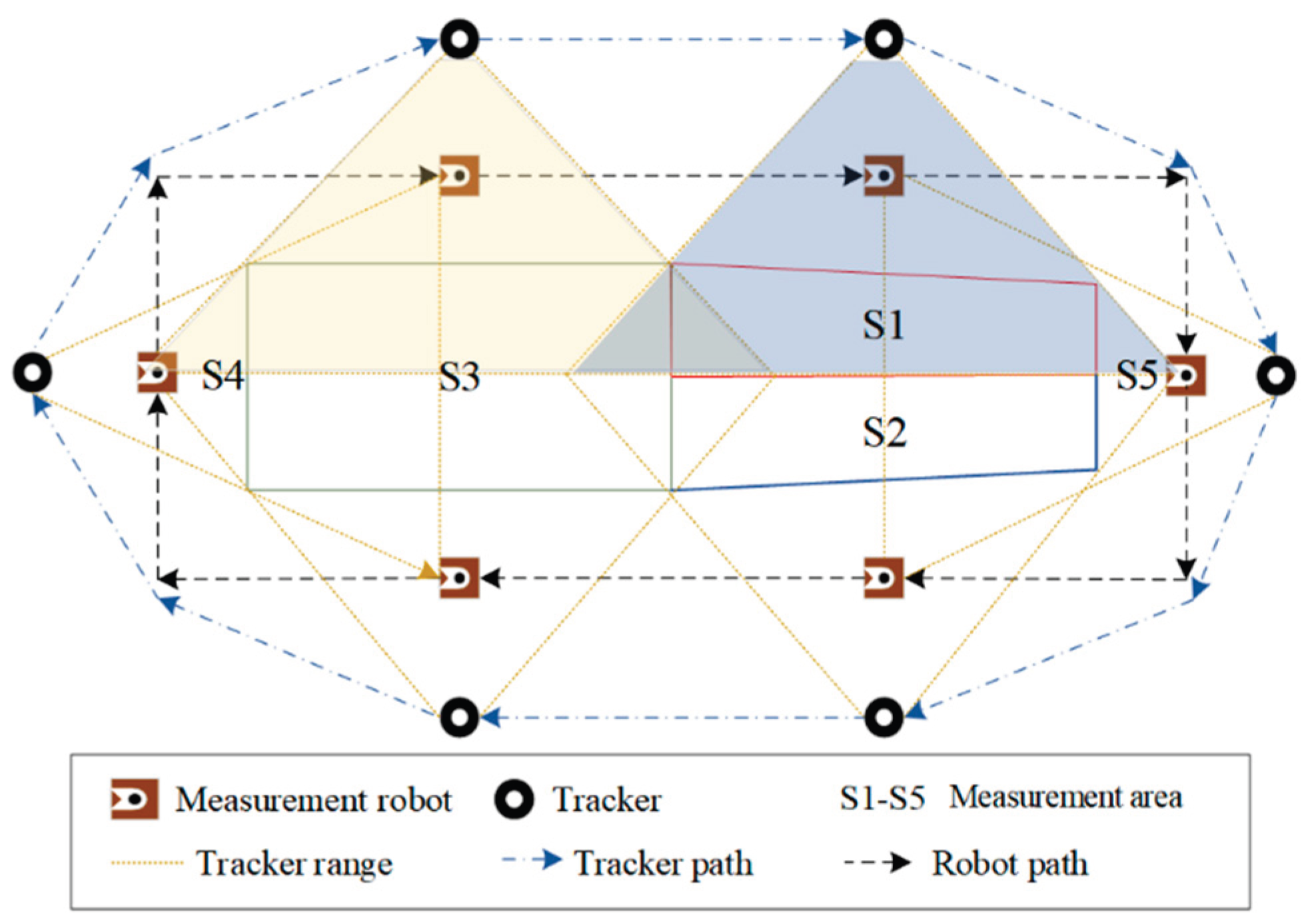
Figure 2.
Dynamic structure analysis of the mobile robot.
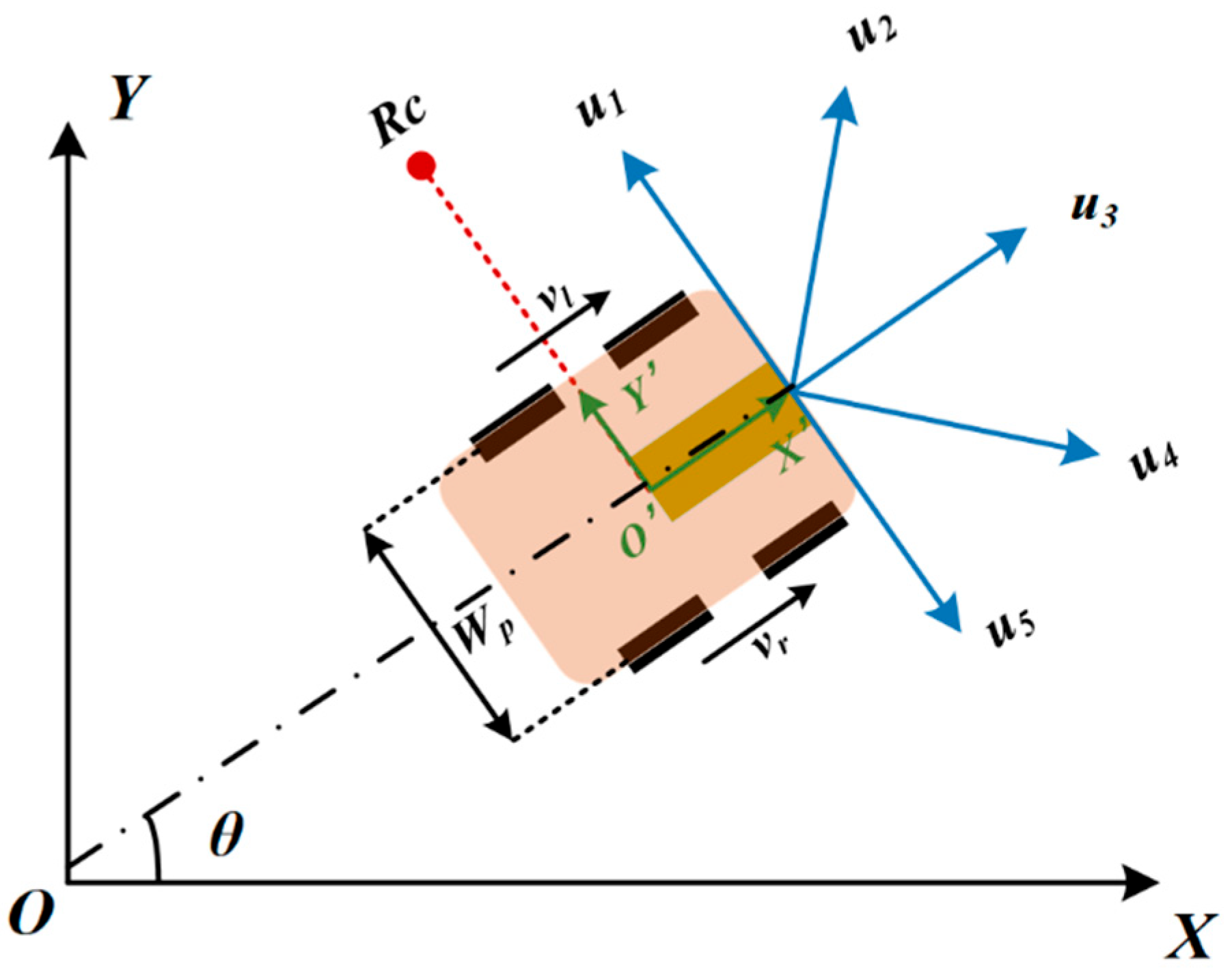
Figure 3.
The framework of proposed algorithm.
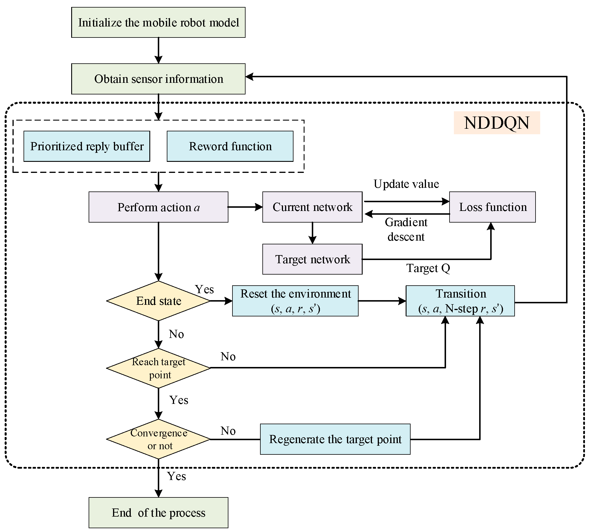
Figure 4.
The average reward value of training in the 10×10 scenario.
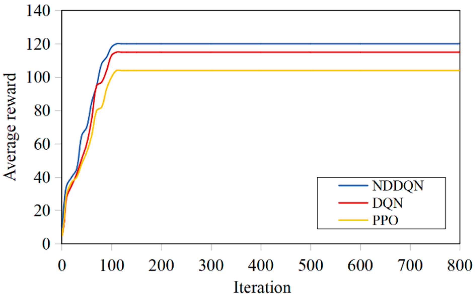
Figure 5.
The average reward value of training in the 20×20 scenario.
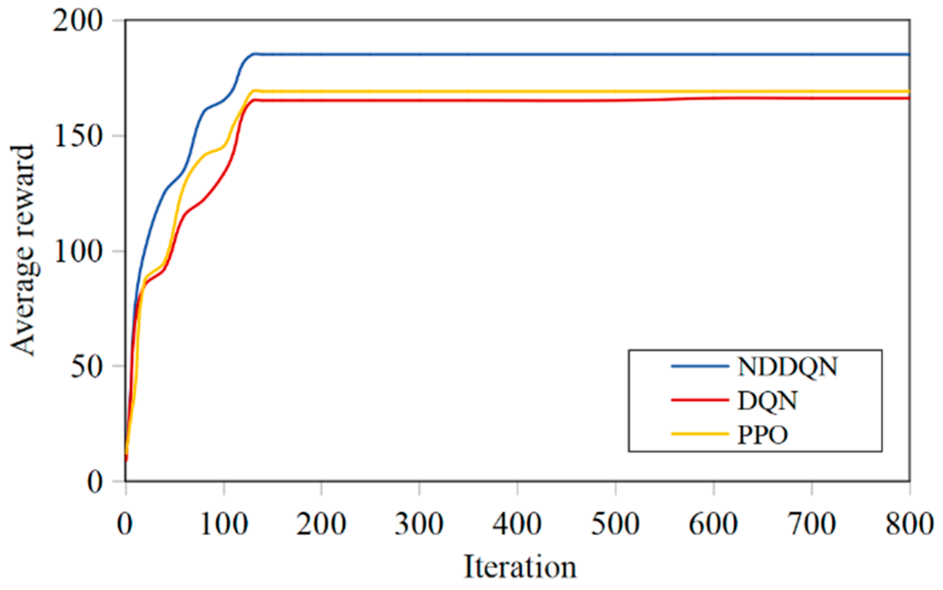
Figure 6.
The average reward value of training in the 30×30 scenario.
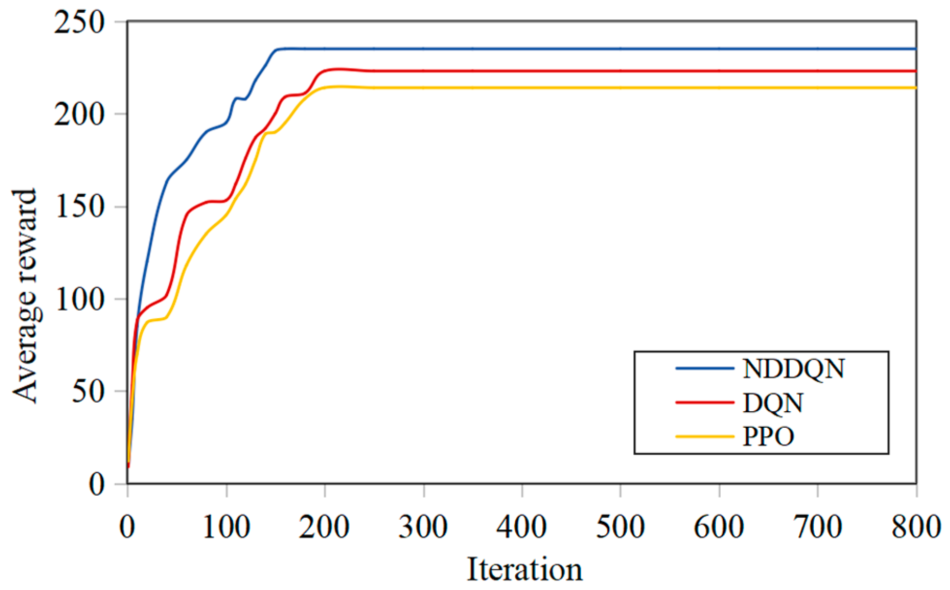
Figure 7.
The 10×10 raster simulation results of three algorithms.
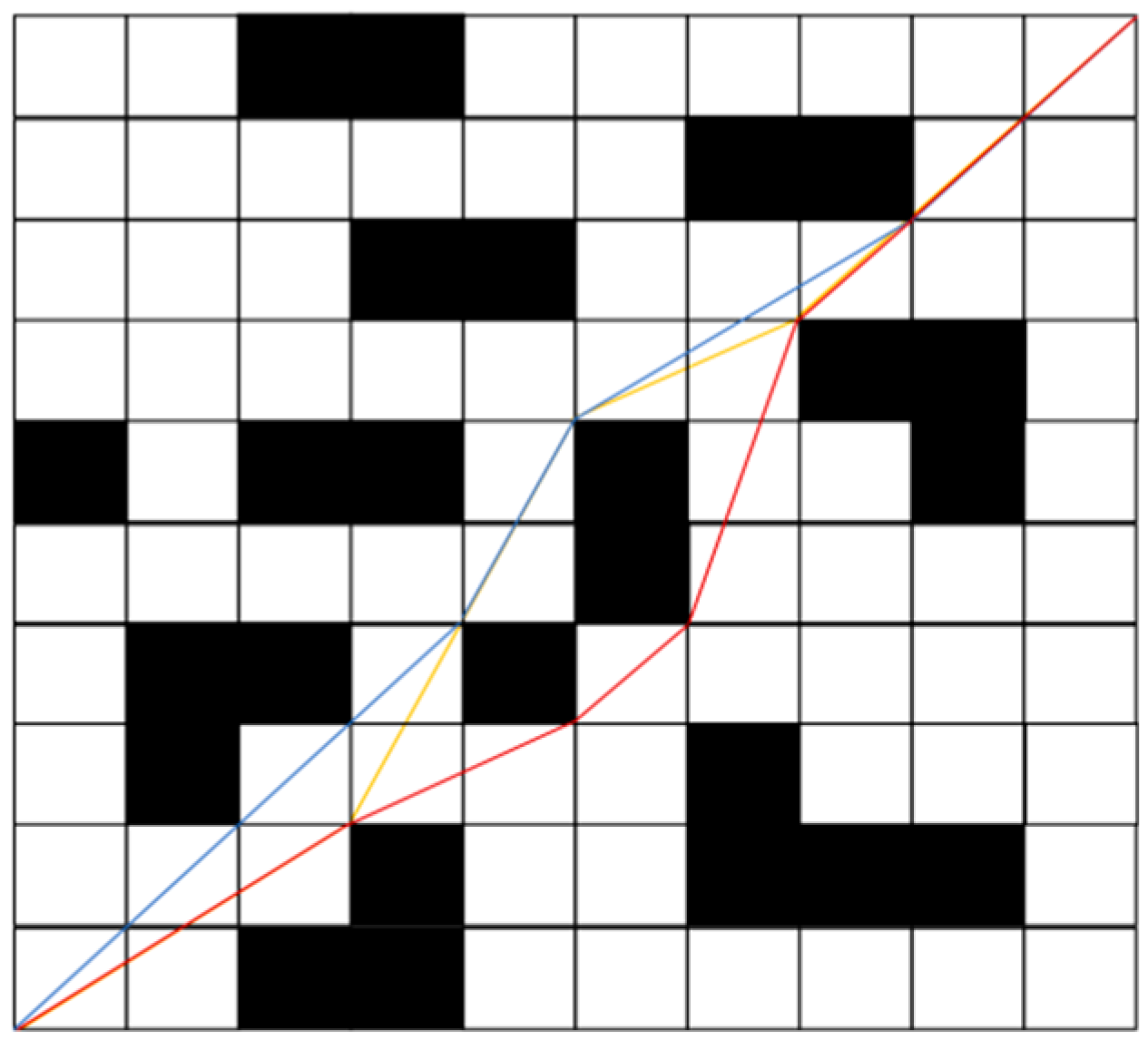
Figure 8.
The 20×20 raster simulation results of three algorithms.
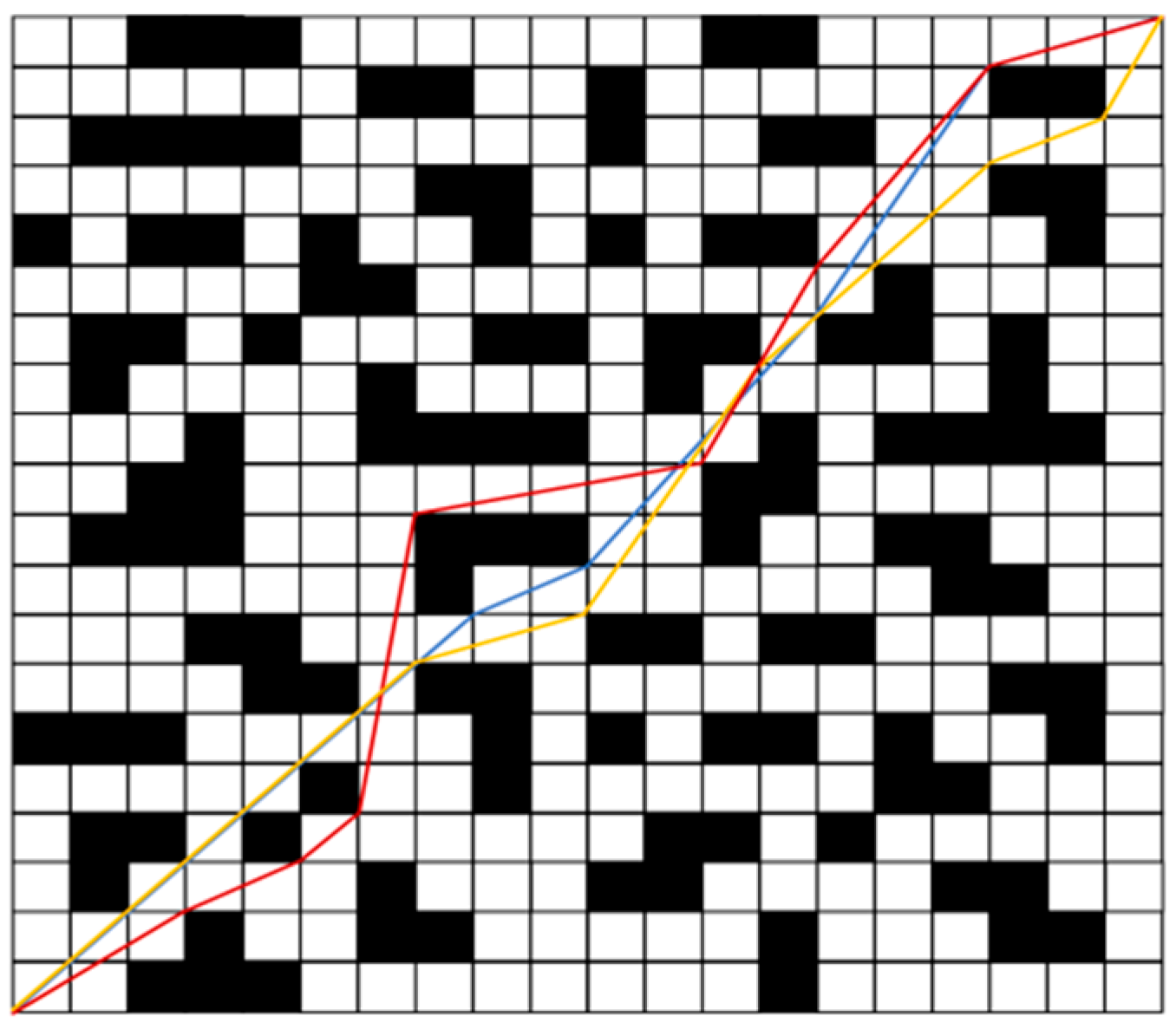
Figure 9.
The 30×30 raster simulation results of three algorithms.
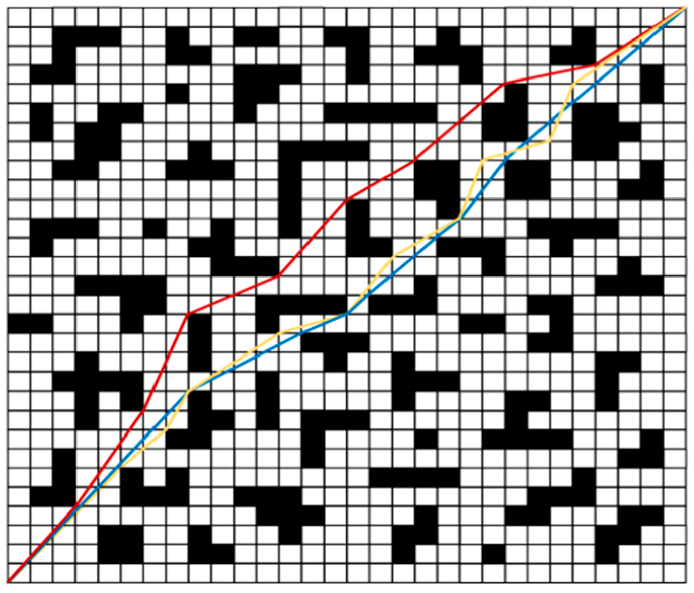
Figure 10.
Generated path for NDDQN algorithm in E1.
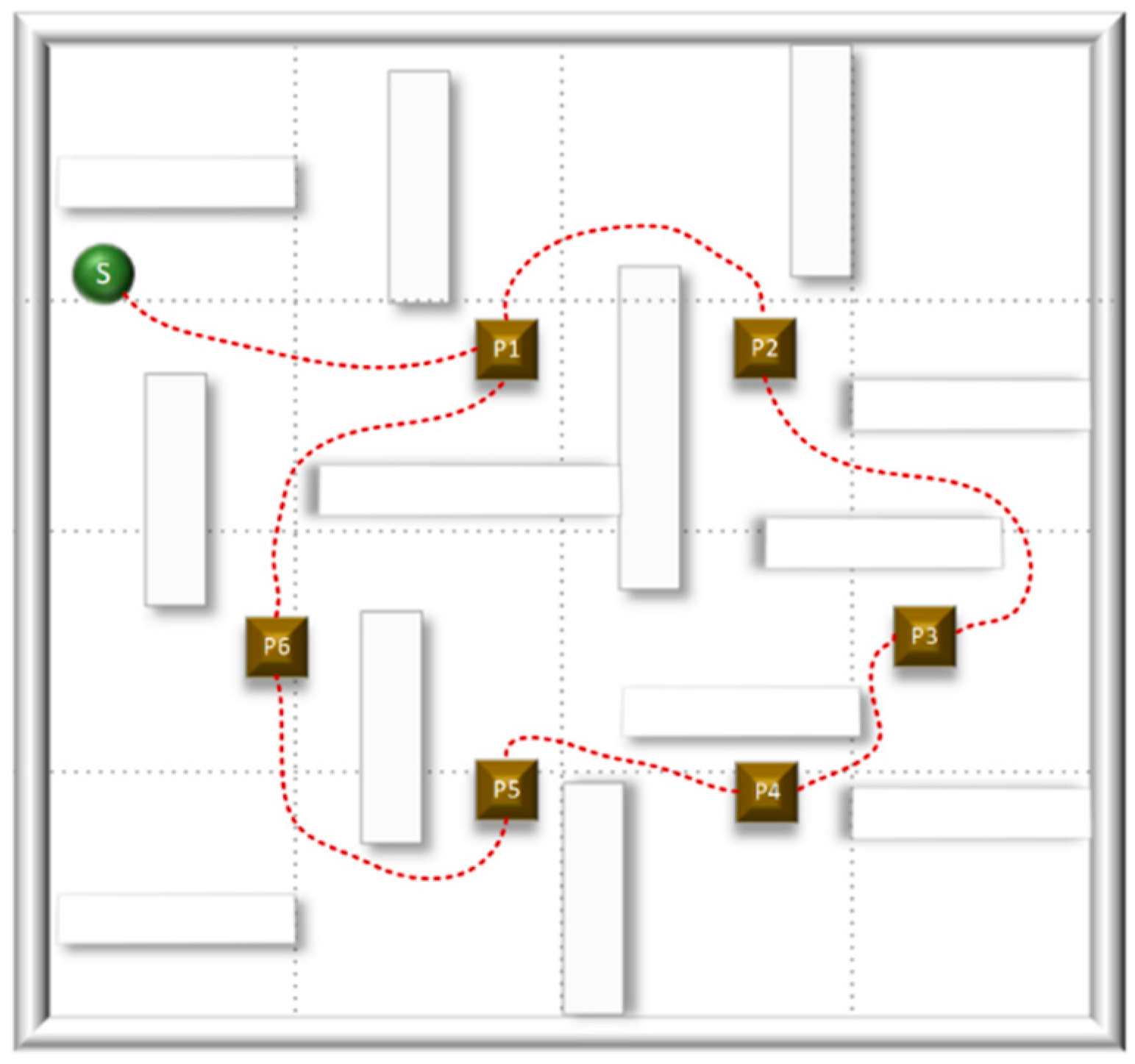
Figure 11.
Generated path for NDDQN algorithm in E2.
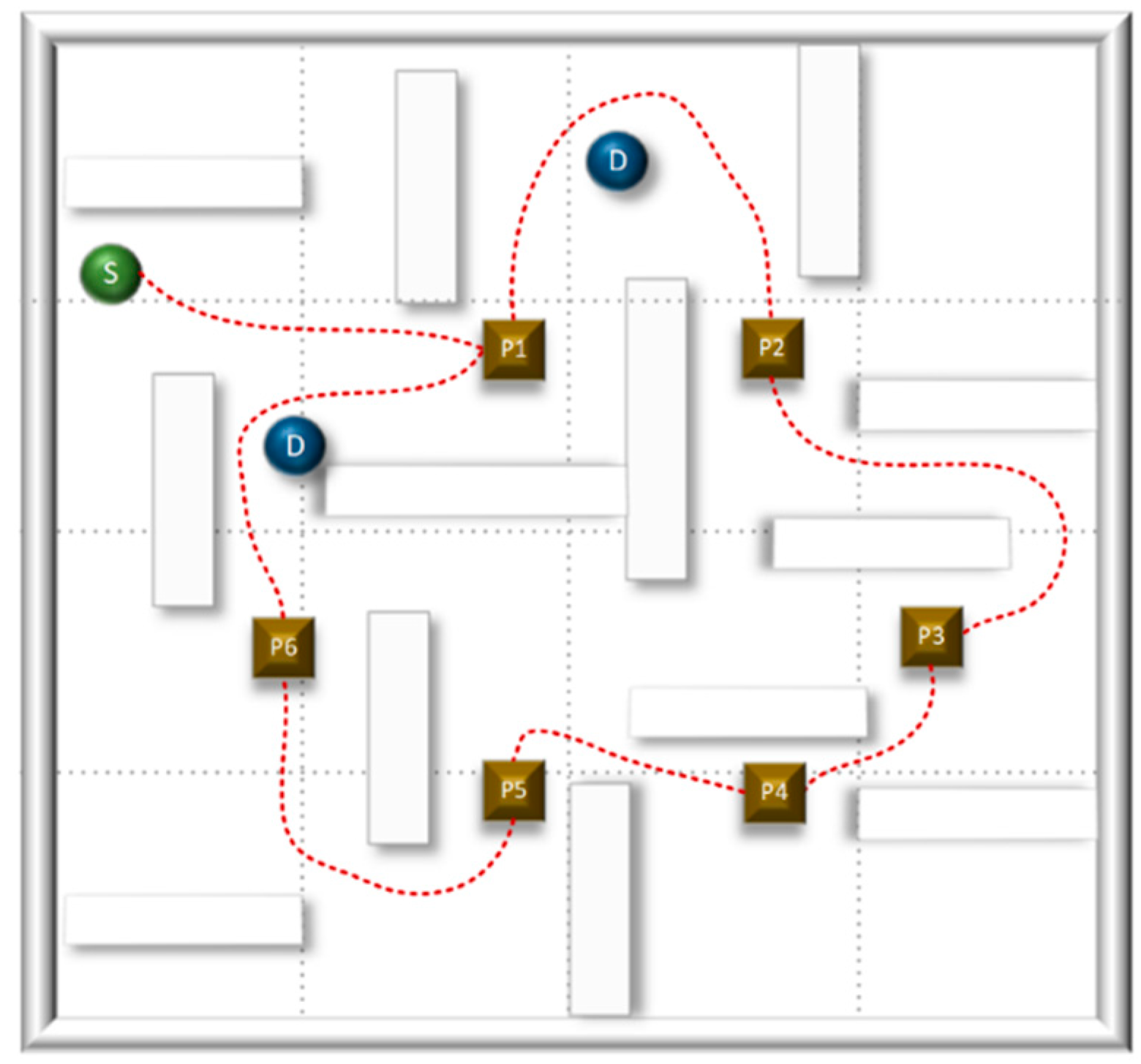
Figure 12.
The robot’s reward for each episode based on PPO algorithm.
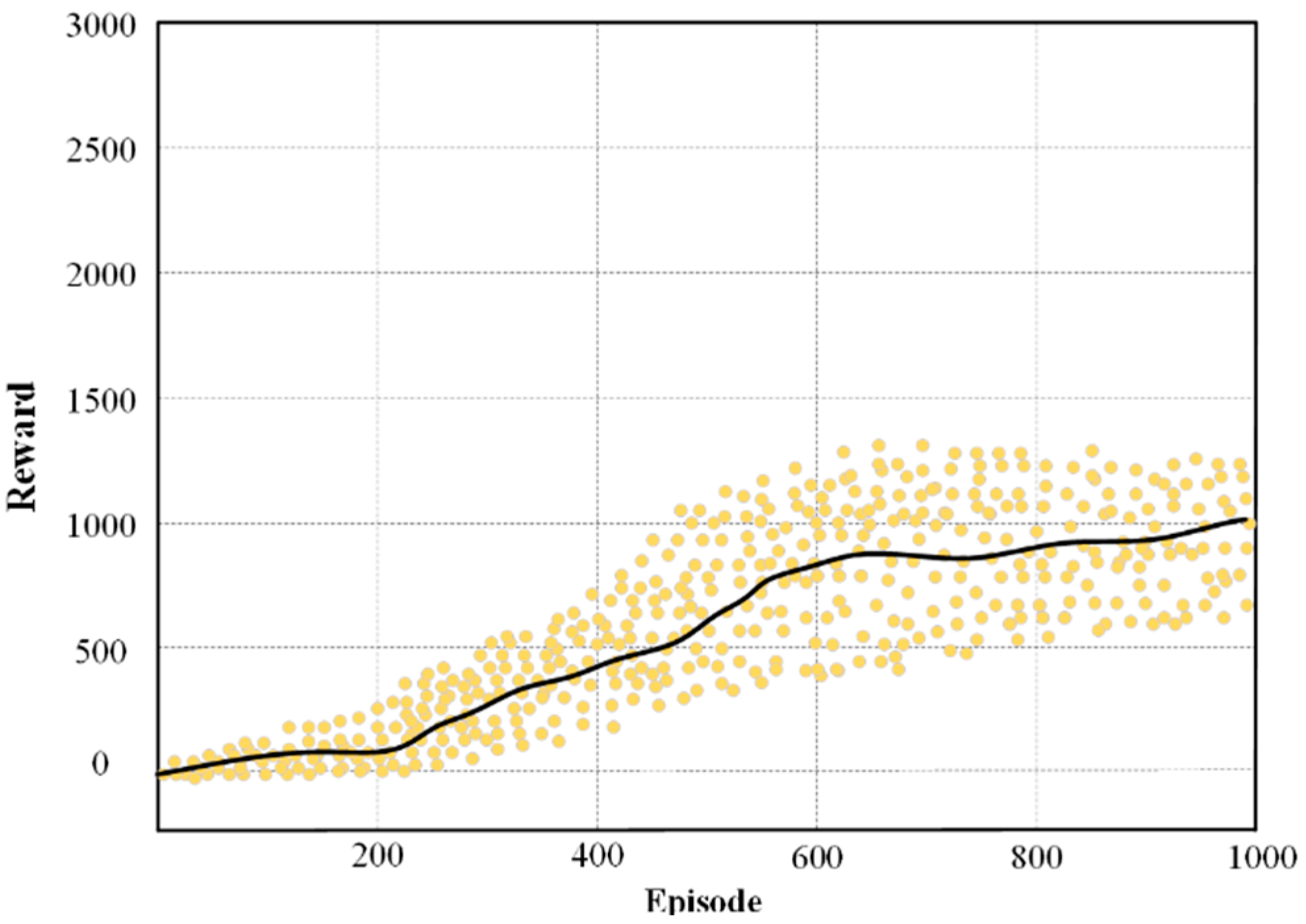
Figure 13.
The robot’s reward for each episode based on DQN algorithm.
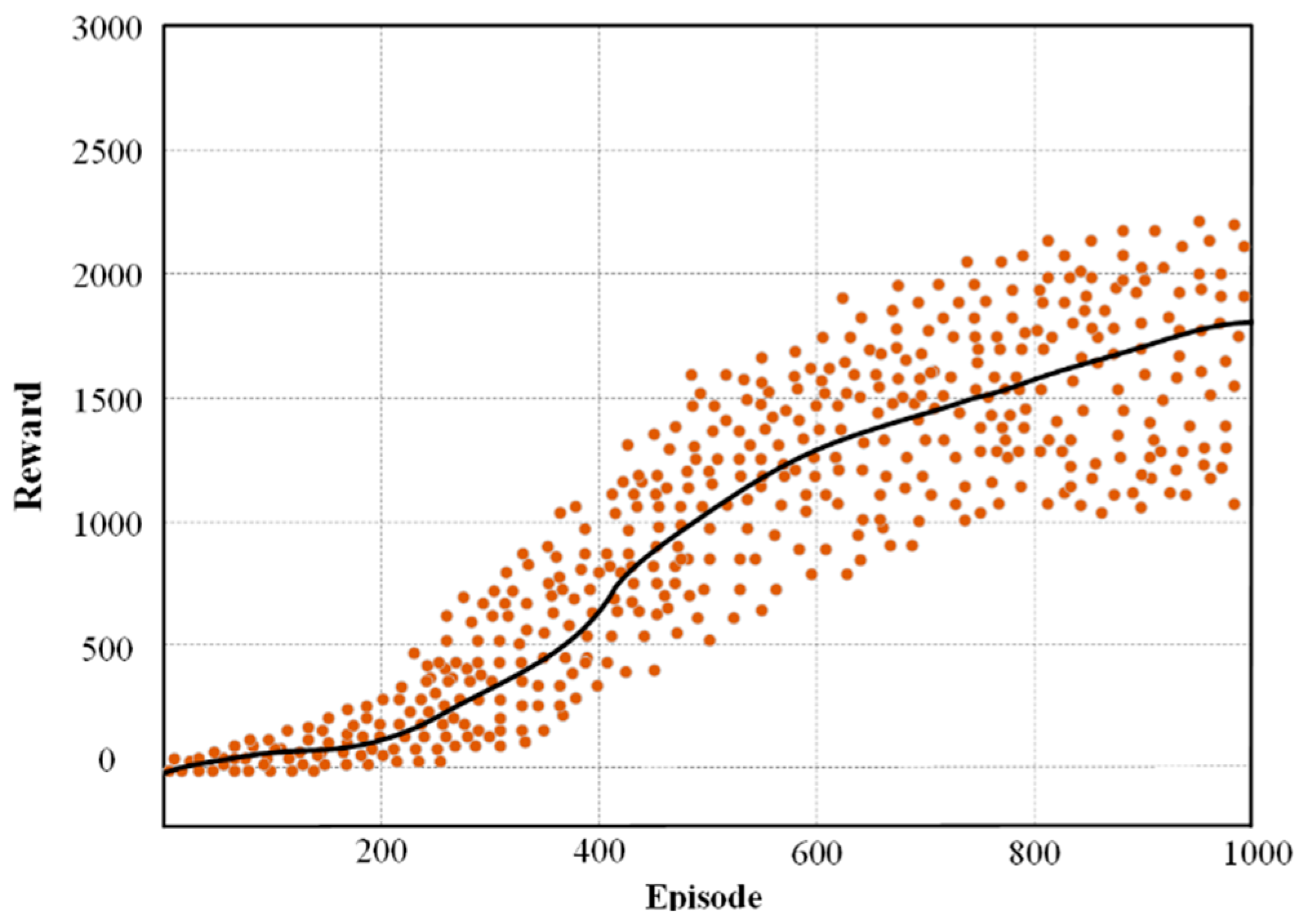
Figure 14.
The robot’s reward for each episode based on NDDQN algorithm.
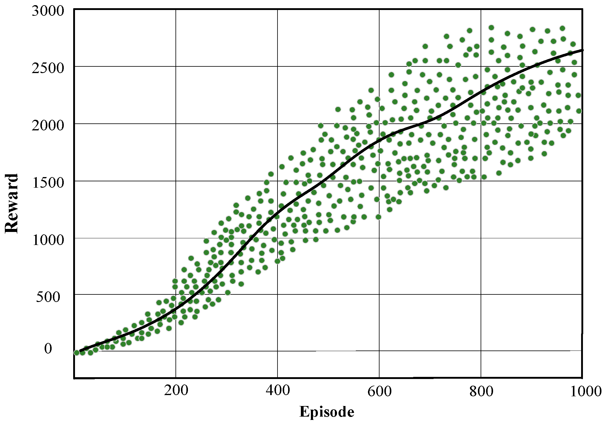

Table 1.
This NDDQN Hyperparameters.
| Hyperparameter | Value |
| The first layer network nodes | 256 |
| The second layer network nodes | 256 |
| The third layer network nodes | 128 |
| Max episodes | 1000 |
| Max steps | 800 |
| Learning rate (α) | 0.0005 |
| Mini-batch | 64 |
| Discount factor (γ) | 0.95 |
| Network update rate | 0.001 |
| The safe distance | 0.5m |
| Playback cache storage capacity | 50000 |
Table 2.
Robot Actions and Corresponding Speed.
| Action | Linear Velocity (v) | Angular Velocity (ω) |
| Move forward | 0.8 m/s | 0 rad/s |
| Turn left | 0.8 m/s | -0.5 rad/s |
| Turn right | 0.8 m/s | 0.5 rad/s |
| Turn left quickly | 0.8 m/s | -1 rad/s |
| Turn right quickly | 0.8 m/s | 1 rad/s |
Table 3.
Path-solving Performance Indicators of Different Example.
| Grid | Algorithm | Total reward | Time | Total length | Number of turns | Average curvature |
| 10×10 | NDDQN | 121 | 19.41 | 14.33 | 3 | 4.2 |
| DQN | 115 | 19.69 | 14.55 | 3 | 4.4 | |
| PPO | 104 | 20.33 | 14.66 | 4 | 5.8 | |
| 20×20 | NDDQN | 183 | 38.46 | 28.78 | 5 | 3.8 |
| DQN | 166 | 38.78 | 29.02 | 5 | 4.1 | |
| PPO | 169 | 41.31 | 30.25 | 7 | 5.2 | |
| 30×30 | NDDQN | 233 | 53.06 | 40.05 | 7 | 3.9 |
| DQN | 221 | 57.40 | 42.32 | 10 | 5.5 | |
| PPO | 214 | 57.96 | 43.17 | 9 | 4.8 |
Table 4.
Comparison of Three Algorithms on Different Environments.
| Method | Success Rate | Convergence Time/Min | ||
| E1 | E2 | E1 | E2 | |
| PPO | 34.2 | 28.4 | 248 | 286 |
| DQA | 58.3 | 49.2 | 153 | 193 |
| NDDQA | 92.7 | 88.6 | 114 | 142 |
Table 5.
Quantitative comparison of ablation experiment results.
| Model | Average Returns | Training Steps | Standard Deviation |
| -N-step | 450.2 ± 25.1 | 55,80 ± 6,50 | 25.1 |
| -PER | 420.5 ± 45.7 | 72,10 ± 8,90 | 45.7 |
| -DQL | 485.3 ± 22.5 | 41,00 ± 5,00 | 22.5 |
| Baseline DQN | 400.8 ± 52.0 | >100,00 | 52.0 |
| NDDQN | 00.0 ± 15.3 | 38,500± 4,20 | 15.3 |
Disclaimer/Publisher’s Note: The statements, opinions and data contained in all publications are solely those of the individual author(s) and contributor(s) and not of MDPI and/or the editor(s). MDPI and/or the editor(s) disclaim responsibility for any injury to people or property resulting from any ideas, methods, instructions or products referred to in the content. |
© 2025 by the authors. Licensee MDPI, Basel, Switzerland. This article is an open access article distributed under the terms and conditions of the Creative Commons Attribution (CC BY) license (http://creativecommons.org/licenses/by/4.0/).
Copyright: This open access article is published under a Creative Commons CC BY 4.0 license, which permit the free download, distribution, and reuse, provided that the author and preprint are cited in any reuse.


