Research on Steel Production Scheduling Optimization Based on Deep Learning

Huayu Zhao; Yixue Chen; Bo Dang; Xiangzhou Jian

doi:10.20944/preprints202412.1502.v1

Submitted:

17 December 2024

Posted:

18 December 2024

You are already at the latest version

Abstract

Steel production scheduling represents a pivotal aspect of the steel manufacturing process, encompassing the strategic allocation of resources and the optimization of production processes. This directly impacts the efficiency and cost-effectiveness of the production process. However, conventional scheduling optimization techniques are ill-equipped to address the intricate nuances of the steel production environment and the deluge of real-time data. In this work, a method of steel production scheduling optimization based on deep reinforcement learning was proposed and subsequently innovated and optimized. The Deep Q Network (DQN) was employed as the fundamental model, with the objective of enhancing the stability and convergence speed of the model. This was achieved through the design of the state space and action space of production scheduling, as well as the incorporation of experience playback and target networks. With regard to model optimization, an adaptive adjustment mechanism of the reward function is proposed, which enables the model to balance the optimization of multiple objectives, such as production efficiency and energy consumption, with greater accuracy. Furthermore, the network structure has been enhanced and a multi-head attention mechanism has been incorporated to augment the model's capacity for scheduling decisions in intricate production scenarios. The optimized model was subjected to experimental verification on an actual steel production dataset, and its performance in terms of scheduling efficiency and resource allocation accuracy was found to be excellent.

Keywords:

Steel production scheduling

;

Deep reinforcement learning

;

Deep Q network (DQN)

;

Reward function optimization

;

Multi-head attention mechanism

Subject:

Computer Science and Mathematics - Artificial Intelligence and Machine Learning

I. Introduction

The integration of advanced information technology has transformed steel production scheduling, enabling intelligent and interconnected manufacturing environments. In the era of smart manufacturing, artificial intelligence (AI) has become a key enabler, integrating seamlessly with production systems to enhance decision-making, optimize resource allocation, and improve efficiency. The convergence of AI and advanced manufacturing has accelerated the adoption of technologies such as real-time data analytics, machine learning, and deep reinforcement learning to address the complexities of modern steel production scheduling.

Steel production dispatching systems now feature enhanced information acquisition, transmission, and processing capabilities, characterized by ubiquity and temporal continuity [1]. AI-powered systems integrate production scheduling with enterprise management, production control, and data monitoring, creating an interconnected ecosystem aligned with Industry 4.0 principles. Extending to physical production sites, these systems enable more comprehensive and responsive scheduling.

Real-time disruptions, such as equipment failures, resource shortages, and order changes, frequently render traditional schedules infeasible. AI addresses these challenges through real-time data processing, predictive analytics, and adaptive scheduling, which are particularly vital for large-scale steel enterprises operating in dynamic environments. Research increasingly focuses on AI’s ability to perceive system states, analyze data, enable collaborative control, and make data-driven decisions within smart manufacturing contexts [2].

Steel production scheduling must adapt to complex scenarios with multiple simultaneous disturbances. Flexible parameter adjustments and dynamic scheduling reconstruction are essential. AI techniques like deep reinforcement learning model complex objectives, constraints, and uncertainties, transforming the traditionally NP-hard scheduling problem into an adaptive, resilient system capable of efficient operation in dynamic environments [3].

Traditional scheduling research has focused on static models and algorithms, which struggle to meet the demands of personalized, multi-variety, low-volume production [4]. AI-enabled solutions overcome these limitations by responding to rapidly changing internal and external factors. Machine learning identifies patterns from historical data, while reinforcement learning optimizes performance in real time.

Conventional approaches, relying on static assumptions, limit flexibility in dynamic production scenarios. AI-powered systems address these challenges by employing techniques such as neural network-based learning and optimization to align scheduling models with real-time conditions [5]. These systems decouple dependencies in traditional scheduling, providing modular and scalable solutions that enable rapid adjustments. This flexibility is critical for balancing mass production with personalized customization. AI thus serves as a cornerstone for developing intelligent, flexible scheduling methods to meet the growing complexity of modern steel manufacturing.

II. Related Work

Bu H N et al. [6] employed case-based reasoning to obtain a high-quality initial solution for cold continuous rolling planning. They then used the Tabu Search (TS) algorithm for global optimization, enhancing the TS algorithm’s search capability, reducing local optima risks, and accelerating convergence. This hybrid approach improved computational efficiency and accuracy, enabling rapid generation of high-quality schedules in complex production environments with significant potential for steel production optimization.

Jiang GZ et al. [7] proposed integrating a knowledge network into a steel production scheduling system, creating a mixed process knowledge network. By establishing a knowledge base (KB) for the steel mixing process, the system integrated multidimensional information such as process flows, equipment status, and scheduling strategies. Their study focused on model matching and reconstruction to adapt scheduling to real production needs. Modular reuse of model knowledge further enhanced adaptability and scalability.

Zahmani MH et al. [8] introduced a method combining scheduling rules, genetic algorithms, data mining, and simulation to improve production scheduling. A genetic algorithm optimized scheduling globally, while data mining extracted key knowledge to identify critical rules and patterns for the scheduling process.

Qiu et al. [9] developed a data mining-based prediction system for disturbances in workshop scheduling. The system comprises three modules: data mining, disturbance prediction, and manufacturing processes. The data mining module identifies production patterns and causes of disturbances by analyzing historical production data.

III. Methodology

A. Deep Q Network

The steel production scheduling problem can be defined as a discrete-time Markov decision process (MDP), which can be represented as a quintuple

(S, A, P, R, γ)

. The term

S

denotes the state space, which encompasses all pertinent system data pertaining to steel production. This includes, but is not limited to, the current status of the production process, the operational status of machinery, the allocation of resources, and so forth.

The action space, represented by

A

, is used for scheduling operations, such as allocating resources to a specific production link and adjusting the processing sequence. The state transition probability, represented by

P (s^{'} | s, a)

, is the probability distribution of transitioning to state QQ after performing action

a

in state

s^{'}

.

The term

R (s, a)

denotes the reward function, which quantifies the immediate reward yielded by the execution of action

a

in state

s

. The reward function can be meticulously devised in accordance with a multitude of objectives, including those pertaining to production efficiency, energy consumption and output. The discount factor, represented by

γ \in [0,1]

, serves to regulate the influence of prospective rewards on present-day decision-making. The objective is to identify an optimal strategy,

π^{*}

, that maximises the expected cumulative reward as Equation (1).

\begin{matrix} π^{*} (s) = a r g \max_{π} E [\sum_{t = 0}^{\infty} γ^{t} R (s_{t}, a_{t})] . \end{matrix}

(1)

The DQN algorithm is employed to address the optimisation challenge associated with steel production scheduling. In DQN, the neural network is employed as an approximate function to represent the

Q

value function

Q (s, a; θ)

, where

θ

represents the parameter of the neural network. In accordance with the Bellman equation, the update rules for the

Q

value function are based on a given state

s

and action

a

described as Equation (2).

Q (s_{t}, a_{t}) = R (s_{t}, a_{t}) + γ \max_{a_{t + 1}} Q (s_{t + 1}, a_{t + 1}; θ^{-}),

(2)

where

θ^{-}

represents the parameter of the target network, which is updated independently from the current network parameter

θ

with the objective of stabilising the training process. The configuration of the state space

S

encompasses pivotal data pertinent to the manufacturing process. The status vector of the production line should be set to

s = [s_{1}, s_{2}, \dots, s_{n}]

. In this context,

s_{i}

represents the status of the first

i

machine in the production line, including its current task load, resource consumption, and dependencies with other machines. The incorporation of this data into the state space enables the capture of the intricate dynamics inherent to steel production.

The action space, designated as

A

, represents the scheduling operations that can be performed at each discrete time step. Let us suppose that there are

m

machines. We define actions as operations which schedule resources from one process to another. The action vector can be expressed as

a = [a_{1}, a_{2}, \dots, a_{m}]

, where

a_{i}

represents the scheduling strategy for the

i

machine.

B. Adaptive Adjustment Mechanism

This subsection presents an innovative approach to improve the stability and convergence speed of the Deep Q Network (DQN). The method combines empirical replay and target network mechanisms with an adaptive reward function adjustment to achieve dynamic multi-objective optimization. The experience replay mechanism archives state transitions

(s_{t}, a_{t},, r_{t}, s_{t + 1})

in a replay buffer during each training cycle. A random sample from the buffer is then used for training during network updates, reducing sample correlation and enhancing model training. The update formula is provided in Equation (3).

\begin{matrix} Q ((s_{t}, a_{t}; θ) = Q ((s_{t}, a_{t}; θ) \\ + α (r_{t} + γ \max_{a^{'}} Q (s_{t + 1}, a^{'}; θ^{-}) - Q ((s_{t}, a_{t}; θ)) . \end{matrix}

(3)

The parameters of the current network are

θ

, while those of the target network are

θ^{-}

. The learning rate is

α

, and the discount factor is

γ

. The parameters of the target network

θ^{-}

are decoupled from the current network

θ

and updated on a fixed interval

C

to enable gradual adaptation to changes in the current network described as Equation (4):

θ^{-} = θ i f t % C = 0 .

(4)

The proposed design circumvents the inherent instability of

Q - v a l u e

estimation, thereby facilitating enhanced convergence of the model. This is particularly beneficial in the context of complex steel production scheduling tasks, where it can mitigate the impact of state transition uncertainty-induced fluctuations.

To achieve a better balance between production efficiency, resource consumption, and cost, this study proposes an adaptive adjustment mechanism for the reward function. Conventional reward functions are fixed, making it difficult to adjust weights for multiple objectives in dynamic production environments. This study introduces an innovative strategy that combines adaptive dynamic weight adjustment with an experience playback mechanism, allowing the reward function weights to be optimized based on actual production conditions. The reward function

R (s, a)

comprises multiple sub-goals, including productivity, energy consumption, and cost, as shown in Equation (5).

\begin{matrix} R (s, a) = w_{1} (t) R_{e f f i c i e n c y} (s, a) \\ + w_{2} (t) R_{e n e r g y} (s, a) + w_{3} (t) R_{c o s t} (s, a) . \end{matrix}

(5)

The weights assigned to production efficiency

w_{1} (t)

, energy consumption

w_{2} (t)

, and cost

w_{3} (t)

are subject to dynamic adjustment over time. The core of the adaptive adjustment mechanism is the real-time modification of individual weights in accordance with feedback. The weights are defined as follows, as illustrated in Equation (6).

w_{i} (t + 1) = w_{i} (t) + η_{i} \cdot ∆ R_{i} (t),

(6)

where

η_{i}

represents the learning rate, while

∆ R_{i} (t)

denotes the discrepancy between the immediate and anticipated rewards associated with the

T

sub-goal as illustrated in Equation (7).

∆ R_{i} (t) = {\hat{R}}_{i} (t) - R_{i} (t),

where

{\hat{R}}_{i} (t)

signifies the expected reward for sub-goal

i

, whereas

R_{i} (t)

denotes the immediate reward actually received. The feedback mechanism enables the model to adjust the balance of multiple objectives in each training cycle, thereby allowing it to optimise dynamically between competing goals such as production efficiency and energy consumption.

To ensure optimal model performance, key parameters were tuned during preliminary experiments. The learning rate α was tested in the range [0.001, 0.1], and the discount factor γ was varied between 0.8 and 0.99. Additionally, the initial reward weights (λp, λe, λc) were set equally and adjusted dynamically during training. These adjustments helped balance objectives like production efficiency, energy consumption, and cost.

IV. Experiments

A. Experimental Setups

The characteristic indicators of multiple disturbance events in the steel production process are employed as input, with strong disturbance and weak disturbance serving as the output of the decision tree model. The data were sourced from the following: The data were sourced from the steel mill workshop Manufacturing Execution System (MES) database. The decision parameter, designated as D, represents the intensity of the disturbance. This parameter is defined in terms of two distinct classifications: A value of 1 is assigned to indicate a weak disturbance, while a value of 2 is assigned to indicate a strong disturbance. A decision tree model is constructed from these characteristic indicators with the objective of distinguishing and predicting perturbations of different intensities. The model was trained on an NVIDIA Tesla V100 GPU, requiring approximately 12 hours for 50,000 iterations. Resource demands were significant, highlighting the need for hardware efficiency.

B. Experimental Analysis

Prediction accuracy metrics evaluate a model’s ability to correctly identify or classify outcomes in a prediction task. Figure 1 compares the experimental prediction accuracy of TS (Tabu Search), KB (Knowledge-Based Algorithm), and our method. The horizontal axis represents the number of algorithm runs. As shown, our method achieves higher prediction accuracy and faster convergence compared to the other two methods. Table 1 presents initial data for molten steel production scheduling, including processing, start, and end times. Figure 2 shows a Gantt chart of production scheduling generated by TS, KB, and our proposed method. It depicts processing times and task schedules for each heat on different equipment. Colors represent various heats, the horizontal axis indicates time (minutes), and the vertical axis lists devices, showing task start and end times on each device.

The TS method uses neighborhood search to avoid some local optima but may result in inflexible task scheduling. In more complex scenarios, it often leads to scheduling delays or uneven resource allocation. The KB method schedules tasks based on predefined rules, such as prioritizing specific devices, which can cause delays for others. In contrast, our proposed deep reinforcement learning approach adapts intelligently to environmental changes, balances task allocation across devices, and improves scheduling efficiency and robustness.

Sensitivity analysis revealed that a learning rate of 0.01 provided the best trade-off between convergence speed and stability, while γ=0.95 effectively balanced short and long term rewards. The adaptive reward mechanism outperformed fixed-weight configurations, ensuring dynamic trade-offs among objectives. However, the method’s computational requirements may limit industrial deployment. Techniques such as model pruning or quantization could reduce costs while maintaining performance.

V. Conclusion

In conclusion, our comparative analysis of TS, KB, and the proposed deep reinforcement learning-based method highlights their respective strengths and limitations. TS avoids local optima but struggles with resource imbalances in complex scenarios, while KB offers faster scheduling but lacks adaptability to real-time changes. Our method demonstrates superior scheduling efficiency and resilience, effectively handling multi-disturbance events and dynamic constraints. For practical deployment, challenges such as integration with existing MES systems, real-time data handling, and operator usability must be addressed. Future work will focus on pilot studies to validate its feasibility in real steel production environments.

References

Rosyidi, Cucuk Nur, Shanella Nestri Hapsari, and Wakhid Ahmad Jauhari. “An integrated optimization model of production plan in a large steel manufacturing company.” Journal of Industrial and Production Engineering 38.3 (2021): 186-196. [CrossRef]
Yonaga, Kouki, et al. “Quantum optimization with Lagrangian decomposition for multiple-process scheduling in steel manufacturing.” Isij International 62.9 (2022): 1874-1880. [CrossRef]
Iannino, Vincenzo, et al. “A hybrid approach for improving the flexibility of production scheduling in flat steel industry.” Integrated Computer-Aided Engineering 29.4 (2022): 367-387. [CrossRef]
Merten, Daniel, et al. “Novel genetic algorithm for simultaneous scheduling of two distinct steel production lines.” Steel 4.0: Digitalization in Steel Industry. Cham: Springer International Publishing, 2024. 167-187.
Che, Gelegen, et al. “A deep reinforcement learning based multi-objective optimization for the scheduling of oxygen production system in integrated iron and steel plants.” Applied Energy 345 (2023): 121332. [CrossRef]
Bu, He-nan, Zhu-wen Yan, and Dian-Hua Zhang. “Application of case-based reasoning-Tabu search hybrid algorithm for rolling schedule optimization in tandem cold rolling.” Engineering Computations 35.1 (2018): 187-201. [CrossRef]
Jiang, Guozhang, et al. “Model knowledge matching algorithm for steelmaking casting scheduling.” International Journal of Wireless and Mobile Computing 15.3 (2018): 215-222.
Habib Zahmani, Mohamed, and Baghdad Atmani. “Multiple dispatching rules allocation in real time using data mining, genetic algorithms, and simulation.” Journal of Scheduling 24.2 (2021): 175-196.
Qiu, Yongtao, et al. “Data mining–based disturbances prediction for job shop scheduling.” Advances in Mechanical Engineering 11.3 (2019): 1687814019838178. [CrossRef]

Figure 1. Comparison of Prediction Accuracy Over Algorithm Runs.

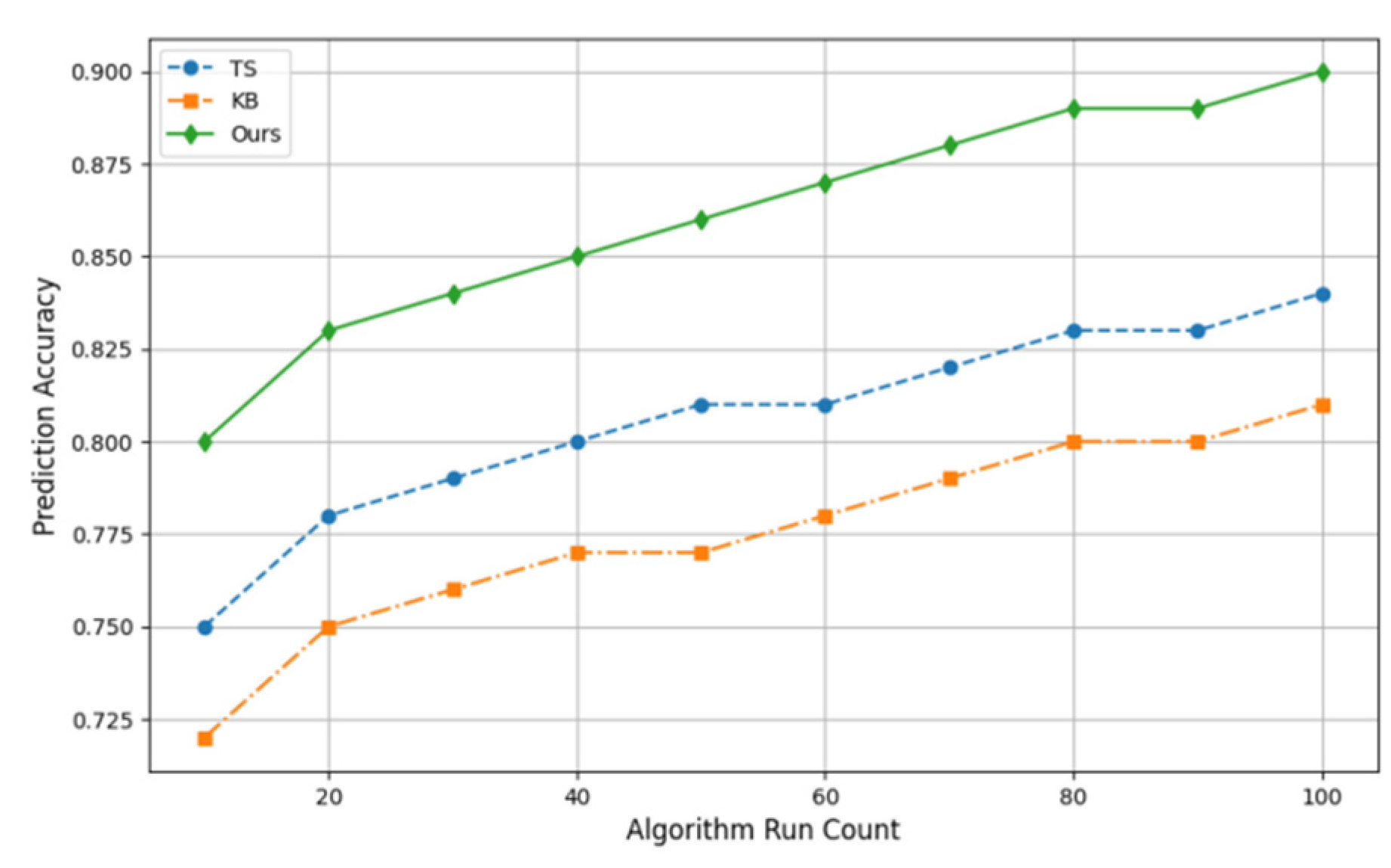
Figure 2. Scheduling Results Illustration using Gantt chart.

Table 1. Initial Production Schedule.

	Furnace	Equipment	Start Time	Processing Time	End Time
0	Furnace_1	Equipment_1	95	65	160
1	Furnace_1	Equipment_2	471	25	496
2	Furnace_1	Equipment_3	232	56	288
3	Furnace_1	Equipment_4	179	43	222
4	Furnace_1	Equipment_5	112	65	177
5	Furnace_1	Equipment_6	317	72	389
6	Furnace_1	Equipment_7	496	79	575
7	Furnace_1	Equipment_8	441	82	523
8	Furnace_1	Equipment_9	51	51	102
9	Furnace_1	Equipment_10	267	52	319

Disclaimer/Publisher’s Note: The statements, opinions and data contained in all publications are solely those of the individual author(s) and contributor(s) and not of MDPI and/or the editor(s). MDPI and/or the editor(s) disclaim responsibility for any injury to people or property resulting from any ideas, methods, instructions or products referred to in the content.

© 2024 by the authors. Licensee MDPI, Basel, Switzerland. This article is an open access article distributed under the terms and conditions of the Creative Commons Attribution (CC BY) license (http://creativecommons.org/licenses/by/4.0/).

Copyright: This open access article is published under a Creative Commons CC BY 4.0 license, which permit the free download, distribution, and reuse, provided that the author and preprint are cited in any reuse.

Research on Steel Production Scheduling Optimization Based on Deep Learning

Abstract

Keywords:

Subject:

I. Introduction

II. Related Work

III. Methodology

A. Deep Q Network

B. Adaptive Adjustment Mechanism

IV. Experiments

A. Experimental Setups

B. Experimental Analysis

V. Conclusion

References

MDPI Initiatives

Important Links

Subscribe