
Submitted:
20 November 2024
Posted:
26 November 2024
You are already at the latest version
Abstract
Warehouses play a vital role in logistics systems, not only for storing goods but also for provid-ing value-added services. To improve warehouse productivity and reduce costs, it is essential to measure their performance and identify inefficiencies. This paper introduces a new aggregated Key Performance Indicator (KPI), called Overall Warehouse Effectiveness (OWE), to evaluate the effectiveness of the physical structure of a warehouse. OWE utilizes the concepts of Availability, Performance, and Quality, similar to the Overall Equipment Effectiveness (OEE) metric used in manufacturing. The proposed indicator is then applied to a case study to demonstrate its use and provide theoretical and practical implications. In terms of theoretical implications, the proposed metric fills a gap in the literature by providing an aggregated indicator specifically designed for storage systems. For practitioners, OWE enables the identification of waste, customer service faults and adequacy of inventory management policies.
Keywords:
OEE
; Warehouse Performance
; KPIs
; Performance measurement
1. Introduction
The expanding globalization, the advancement of the world economy and developing industrialism of consumer orders have prompted an increased demand for logistics services [1]. This environment is characterized by strong competition and increasingly demanding customers’ requirements in terms of punctuality and timeliness of deliveries, which leads to a reduction of margins for global logistics companies [2].
The role of warehouses for logistics services is crucial because they contribute significantly to the storage of goods from the time of production until the goods are supplied to consumers on demand. In the highly competitive business environment of today, a warehouse is not just a place to store inventory but also to manage and operate value-added services [3]. Warehouses are therefore one of the most relevant items for overall firm performance [4]. This scenario requires companies to continuously search for systems and methods to increase the productivity of their warehouse and thus contain costs, while using the same number of resources.
In order to improve any system, it is essential to measure the actual performance of the system and identify waste and inefficiencies [5]. Measurement is the initial and most basic step for achieving improvements in an organization and is also a vital component of continuous improvement [6,7]. The first step of a warehouse performance measurement process is identifying the right key performance indicators (KPIs) and prioritizing them based on industry-specific contexts [8]. Several warehouse KPIs have been put forward by scholars in recent years, such as productivity, space utilization, cycle time, and cost (see [9] for a comprehensive literature review).
While individual metrics such as inventory accuracy, order fulfillment rates, on-time delivery, and employee productivity are essential for evaluating specific aspects of warehouse performance, an aggregated performance indicator can provide a comprehensive view of the overall effectiveness of the warehouse. Several aggregated performance measurement indicators are available in the literature for manufacturing processes, among which the most used is OEE [10]. The OEE indicator is one of the most efficient indicators that can authentically measure the operational performance within production system and is used to benchmark, analyze and improve any production process [11]. Furthermore, the OEE provides a quantitative metric for measuring the performance of not just individual equipment, but also of entire processes [12]. OEE thus became a pillar for continuous improvement strategy of companies operating in completely different sectors such as automotive [13], semiconductor industry [14], metal industry [15], rails [16], airbag safety devices to the automotive industry [17] and in food industry [18,19].
However, only a handful of aggregated indicators are available to study the performance of logistics assets, and they are mainly focused on material handling assets [23].
The objective of this paper is to define a new, aggregated, synthetic Overall Warehouse Effectiveness (OWE) KPI that allows to analyze the effectiveness of the physical structure of the warehouse and thus identifying wastes, faults in the customer service level, adequacy of the inventory management policy and finally areas for improvement. As a matter of fact, warehouse productivity is affected by several underlying factors such as warehouse layout, information system, labour, and equipment [22]. To this end, the OEE is used as a foundation to evaluate the overall performance of a specific resource of the warehouse that was previously overlooked, namely the warehouse rack.
The paper is structured as follows. First, a review of the indicators used in literature to measure warehouse performance as well as of previous applications of the OEE, both in the manufacturing and logistics sectors, is presented. Then, the research approach and the mathematical formulations underlying the OWE are proposed. After, the new KPI is applied to a case study to discuss its use and provide theoretical and practical implications. Finally, conclusions are drawn.
2. Literature Review
2.1. Warehouse Performance Indicators
[9] propose a comprehensive review of warehouse productivity performance indicators for the measurement of the input of major warehouse resources (labour, equipment, space and information system) within the work area to represent the movement and storage output performance. [22] surveyed warehouse experts and found that Storage Space Utilization and Throughput are the most important KPIs for warehouse productivity. [23] analyzed the performance of warehouses using the 25 key performance indicators (KPI) introduced by [24], grouped into five categories (productivity, financial, cycle time, quality and utilization) where each of these refer to the main warehouse processes, namely Receiving, Putaway, Storage, Order picking and Shipping. In terms of productivity, KPIs such as total number of products shipped per time period are used [25]. In terms of “cycle time”, the most important KPI for the receiving process is “Receipt processing time per receipt”, for the putaway process is “Putaway cycle time”, for the storage is “Inventory days on hand”, for order picking is “Order picking cycle time” and for shipping is “Warehouse order cycle time”. Quality KPIs take note of the existence of faults and failures in all warehouse processes, such as for instance receipts processed accurately [24]. Finally, KPIs for warehouse productivity investigate how efficiently is the warehouse space utilized. One example of such KPI is the Inventory space utilization, namely the rate at which space is occupied for storage [26]. The overall capacity usage of the warehouse is also explored [27].
2.2. Overall Equipment Effectiveness (OEE)
2.2.1. Definition
The OEE, proposed by [10], represents the overall yield of a resource, or set of resources, assessed during the period in which these resources are available. The OEE is a very synthetic index, consisting of a single output, which contains within it a great deal of information regarding the production plant, which is why it is effective in making visible where improvements can be made and the impact of Lean tools aimed at improvement. It is a hierarchy of metrics that measure how effectively a manufacturing operation is realized [28].
The composition of the OEE index makes it possible to identify areas for improvement; in fact, it is a function of three performance indicators, all of which are key to monitoring the proper functioning of a plant [29]:
- availability,
- process performance,
- quality rate
Each component indicates an aspect of the process that can be improved.
The OEE indicator decomposes the performance of a production system into three measurable components: availability, performance, and quality. Each component indicates an aspect of the process that can be improved. The OEE can be applied on multiple levels, to a single workstation, to a single piece of machinery, or applied to an entire department or even the entire plant. The original formulations for the component indices of the OEE indicator are shown in Equations 1-4:
This is a standard definition of the Availability, Performance and Quality indices, corresponding to the classic formulation of the OEE (Figure 1) with a time-based metric.
The same formulas can be declined according to the production flow, defined in a reference period (T):
The OEE formulation supports the identification of losses in the effectiveness of the equipment, which could be classified into several categories ranging from equipment failure and idle times to material losses and rework.
2.2.2. Variations of the OEE in Manufacturing Contexts
Although OEE is traditionally used by practitioners as an operational measure for monitoring production performance, it can also be used as a metric for process improvement activities in other contexts. This has led to broadening of OEE to overall factory effectiveness (OFE), overall asset effectiveness (OAE), overall environmental equipment effectiveness (OEEE), overall greenness performance (OGP), and overall labour effectiveness (OLE) (for a review of alternative use of the OEE see [21]).
[30] pointed out that it is necessary to aim at increasing the performance of the whole factory rather than that of individual tools, and thus coined the term overall factory effectiveness (OFE), which focuses on combining activities and relationships between different machines and processes.
Overall Resources Effectiveness (ORE) is a manufacturing performance measurement system that has been developed by [31] with the objective of providing a more inclusive evaluation than OEE, of a machine or process performance. The main difference between ORE and the traditional OEE is that the first evaluates the overall performance of a machine or process based not only on its availability (A), performance (P) and quality (Q) but also in terms of three more elements that are material efficiency (M), process cost and material cost variations. The integration of these three elements into the traditional overall effectiveness evaluation helps to expand the concept of this measure, and in this way, monitor other factors that can also have a considerable impact on the performance of a machine or process.
In their literature review, [32] highlight that the main difference between the variations of the OEE lies in the types of production losses captured by the measurement tool. In this regard, Overall asset effectiveness (OAE), which has been more extensively applied in practice than in theory, can also accommodate productivity losses that are due to commercial, natural, and environmental reasons.
[33] tested a new process-focused flow performance measure supporting a holistic approach to the manufacturing enterprise called operations flow effectiveness (OFE). The OFE highlights operations management design weaknesses and flow inhibitors that reduce cash flow. In this regard, the conventional OEE measure was extended by including the measurement of quality and delivery reliability of system inputs/outputs to enable the measurement of material flow through the whole system.
[34] proposed a novel methodology called overall material usage effectiveness (OME) that seizes upon OEE’s straightforward and easy-to-use structure to address the problem of measuring the effective use of materials within a factory.
Finally, some scholars have added sustainability to the traditional OEE measures of performance. The Overall Environmental Equipment Effectiveness (OEEE), proposed by [35], adds concept of sustainability based on the calculated environmental impact of the complete product life cycle to the OEE. Nevertheless, the aforementioned index shares the limitations of the original OEE, as it solely focuses on effectiveness at the equipment level, thereby disregarding the evaluation of the entire production system. Sustainability issues also come into play in the Overall Greenness Performance (OGP) by [36]. The Overall Greenness Performance (OGP) metric integrates the principles of lean manufacturing, specifically value-added processes, with the Overall Equipment Effectiveness (OEE) framework. This combination creates a hierarchy of metrics that assess the environmental effectiveness of a manufacturing operation based on the value-added processes that customers are willing to pay for.
2.2.3. Applications of the OEE in Logistics
According to the principles of lean manufacturing, an unnecessary movement of people, information or materials and an excessive storage of material in the logistics areas are considered wastes, with a consequent increase in costs. In order to reduce the wastes in a manufacturing context, any unnecessary transport of materials in the plant and any excessive storage should be reduced. To this end, [20] demonstrated the hypothesis that the OEE metric can also be used for transport facilities such as AGVs, and there is a dependence between machine and transport effectiveness. In their simulations they showed that the OEE metrics can be used for the modelling and productivity evaluation of manufacturing and logistics systems, with the generalization of Overall Factory Effectiveness (OFE) and Overall Transport Effectiveness (OTE).
Furthermore, [38] have proven that the management of internal transporting activities within the production affects the effectiveness of the workstations. The proposed Transportation Measure allowed to identify changes in the process of transporting materials, the reduction of the lead time and waiting time. At the same time, the frequency of transportation requirement to ensure material flow within production system are minimized.
The study of [39] highlights the importance of judging the efficiency and effectiveness of a warehouse department, because this plays a vital role within the supply chain process. The purpose of this analysis is to evaluate the usability of IoT in the warehouse through controlling the Materials Handling Equipment (MHE), using a forklift as the key MHE to analyze the efficiency of IoT KPI in comparison with the existing OEE KPI.
Finally, [21] evaluated the effectiveness of an urban freight transportation system using the OEE metric. In this approach, the quality metric ensures that orders are delivered within the time windows (non-defective), the performance metric causes the speed of the operation to be optimized (i.e., transportation), and the availability metric reduces the non-transportation time (i.e., waiting time and unloading times).
In the literature many works that analyze the OEE in the production and logistics areas are found and several variations to the OEE concept have been proposed (see Table 1). However, few of these works have extended the application of a single KPI in the logistic process, and these are limited to transportation assets such as AGVs. Our research highlighted the lack of works capable of measuring the waste in the management of goods within the storage area. The present work aims to fill this gap.
3. OWE: A New, Encompassing Warehouse KPI
3.1. Research Approach
The purpose of this paper is to define a KPI suitable for logistics resources focusing on the “location storage” resource, similarly to what the OEE represents for manufacturing resources.
In other words, our goal is to build a synthetic KPI called Overall Warehouse Effectiveness (OWE), which evaluates the overall performance of a warehouse. This KPI allows to compare logistics activities carried out in similar field (i.e., benchmarking) and to identify waste and areas for improvement of a specific activity (i.e., baseline analysis).
Within a production process, bounded at the two extremes by the arrival of raw materials and the departure of finished products, it is possible to find many different types of material resources (henceforth referred to simply as resources), among which the most useful for the present discussion are the following:
- Process resources: resources involved in the production cycle.
- Logistics resources: resources that intervene during the storage and transportation of raw materials, semi-finished and finished products.
Just as OEE is used to measure the effectiveness of process resources, OWE is introduced here to provide a similar type of assessment for logistics processes.
Specifically, Table 2 compares the meanings of Availability, Process Performance and Quality for the OEE and OWE
In a warehouse we can identify 3 types of logistics resource: space, equipment and labour [40,41]. Space or static resource contains goods and prevents goods damages. Equipment or dynamic resource are transportation units or material handling systems, move goods between machines and warehouse stations (i.e., space). Both equipment and space resources require labour resources to operate them. Labour, space and equipment resources are all necessary in order to create a complete production planning and control procedure [42]. Contrary to production resources whose function is to transform and create added value, the main function of warehouse resources is to maintain the integrity of the goods stored in the warehouse and make those goods available to the final customer.
In the literature, the efficiency and the effectiveness of internal handling systems, therefore of the dynamic aspect of any logistic area, has been analyzed and estimated as a function of OEE [39], while the analysis of the efficiency and effectiveness of storage systems is lacking. Therefore, in this first dissertation on the OWE it has been decided to focus on the warehouse racks and their saturation. To this end, we will treat the static (i.e., space) resource of the warehouse, namely the storage location. Further research will aim at considering dynamic resources as well.
The parameters which constitute the OWE allow to identify several features of a storing area (Table 3). In particular, the “Availability” parameter analyzes and how the “space” resource of a warehouse is related to the stock to be kept within a certain time interval. This parameter is used to evaluate how far a logistical area deviates from complete saturation of the warehouse, i.e., from that state of total optimisation of the “space” resource. This ideal state of the warehouse with respect to the “space” resource is related to a trade-off between two types of waste: space and over-stocking. On the one hand in fact, the warehouse may be oversized, especially in a fixed storage space allocation. On the other hand, the warehouse may be undersized and therefore not available to store part of the unit loads (ULs) within a certain time interval.
The “Performance” parameter focuses on the average saturation of the “space” resource. The average degree of saturation of storage locations depends on stock management policies; thus, indirectly on the movements and flows of goods in a warehouse. However, input and output flows of a warehouse are not always aligned because not all items have the same “Inventory Turnover ratio” and thus are being handled with different frequencies. In this context, the “Performance” parameter evaluates how long a stock is kept in storage, compared to an ideal, Just-in-time case whereby a complete turnover of all ULs takes place every day.
The third parameter focuses on the quality and deliverability of the ULs handled in the warehouse. Some ULs may be damaged during handling and/or their stationing within the individual storage locations. Furthermore, ULs may also be delivered from the warehouse after the promised date. Therefore, the ‘Quality’ parameter measures the degree of conformity of the Output flows with the Demand within the same time interval. This loss of quality due to the different warehouse resources can be overcome by having an additional stock in the storage area compared to the operational stock, thus affecting the definition of the safety stock.
3.2. Mathematical Formulations
Any warehouse static resource is characterized by three fundamental aspects, as shown in Figure 2:
- input of goods (INPUT)
- time of use of the resource, T
- output of the goods (OUTPUT)
In the discussion of OWE, we choose to use the formulation referring to the output in other words the products leaving the warehouse in a reference time interval T. Thus, the parameters availability, performance and quality will be expressed as output ratios.
The main assumptions for the mathematical formulations are as follows:
- the analysis has a time bucket t equal to one day, meaning that each UL has a minimum theoretical stay in the warehouse equal to one day, but nothing prevents choosing time buckets of a shorter duration.
- i(t) is the input function in time bucket t and is defined in the interval 1 ≤ t ≤ T with t = 1, 2 , ..., T.
- o(t) is the output function in time bucket t and is defined in the interval 1 ≤ t ≤ T with t = 1, 2 , ..., T.
- There is an equivalence between ULs and storage locations, whereby each storage location holds only one UL.
The main variables of the model are defined in Table 4.
The outflow from the warehouse at time T is defined as follows:
Then we can define the components of the OWE using the previous assumptions and definitions.
3.2.1. Availability
The ability of the resource to be available to maintain goods with respect to the actual planning of input and output flows. Considering the characteristics of the warehouse, it can be expressed as the ratio between the maximum manageable theoretical output in the interval T in a warehouse of capacity equal to Imax(T) locations and the maximum manageable theoretical output in the interval T in a warehouse of capacity equal to SC locations. This means that it only evaluates the physical structure of the warehouse.
Where:
- Oth.max (T,Imax): maximum theoretical output needed to handle Imax, which is equal to Imax * T.
- Oth.max (T,SC): maximum theoretical output needed to handle the whole storage capacity, which is equal to SC*T.
It is assumed that each UL has a minimum theoretical stay in the warehouse equal to 1 day and that all storage locations are occupied.
This indicator measures losses due to wasted space, therefore when its value is lower than 1 the warehouse is oversized compared to the actual capacity requirements.
Considering a warehouse with respect to the “space” resource it is possible to identify two types of waste “space” and “over stock”. In the first case, the warehouse turns out to be oversized and a large part of the storage locations turn out to be unused, especially in a fixed storage space allocation. In the second case, the warehouse turns out to be undersized and therefore not available to maintain in an optimal condition a part of LUs in a certain time interval.
The above proposed formulation does not allow for the evaluation of inefficiencies due to an undersized warehouse; the following alternative formulation is proposed to fill the gap:
It allows wastes due to both surplus capacity and its deficit to be evaluated in the same way.
Availability, measured over a sufficiently long time T, in both cases signals a structural discrepancy between the nominal Storage Capacity (SC) and the storage capacity required to contain Imax(T).
3.2.2. Performance
This indicator measures the effectiveness of the service compared to optimal cases of stock management. This indicator is expressed as the ratio between the output from the warehouse in T and the theoretical maximum manageable output in the interval T in a warehouse with a storage capacity equal to Imax(T) locations.
where , is the mean value of o(t) calculated over the interval T.
The parameter P(T) instead measures effectiveness losses due to non-optimised stock and locations flow management. The evaluation is made by comparison with a theoretical minimum dwell time as defined above.
3.2.3. Quality
Capability of the resource to keep intact products available to the customer with complete and timely deliveries. This capability is expressed as the ratio of conforming output to total output, considering only those goods delivered intact and on time and recording any returns as unfinished.
where Oq(T) is referred as a valuable output or valuable flow delivered to the customer, i.e., not damaged, on time from which any returns, etc. have been excluded. This value is recorded at the end of T.
It measures losses due to deviations in quality and punctuality from what the customer requires.
Substituting the different terms into the OWE expression yields:
Ultimately, this expression tells us that OWE is the ratio of how much “we have delivered” net of various losses to the maximum we potentially “could have delivered” with a warehouse of SC capacity. In Figure 3, the OEE has been adapted to the OWE formula.
4. Case Study Application
The proposed calculation example concerns a finished goods warehouse handling 2 products, for each of which a filling function i(t) (INPUT) and a demand function o(t) (OUTPUT) were assumed in a period T equal to 24 elementary units of time. Based on these data and the assumptions that are given below, the indices of Availability, Service Performance, and Quality needed to calculate the Overall Warehouse Effectiveness value were calculated.
For all demand scenarios the following assumptions are made:
- The warehouse has a Storage Capacity of 1,400 locations.
- The input is considered concentrated at the beginning of the elementary unit of time and is realized in LUs.
- The output is considered concentrated at the end of the elementary time unit and is realized in LUs.
- The handling capacity is such that the input and output are realized.
- For product 1 (cod 001), the output (1) is equal to 2,150 LUs in T.
- For product 2 (cod 002) the output (2) is equal to 1,700 LUs in T.
- The total output O(T) is 3,850 LUs in T.
The presented case study is a simulation, but it was conducted using some basic data from an existing company. The company in question operates in the tissue paper market and has a large finished goods warehouse located in northern Tuscany, where finished products processed in various production facilities within the same region are stored. The warehouse operates with a load unit allocation system characterized by having dedicated positions for different types of products. The finished products are stored in palletized load units (Europallet 2) with an average height of 1,800 mm. The shelving is of the drive-through type, serviced by shuttles in the various levels of the lanes. Each lane in the shelves has an average of 5 levels, and each lane has an average of 8 locations, according to the actual dimensions of the load units. The inbound and outbound flows were modified from their actual trend to amplify the effects on the calculations of the factors of the proposed parameter.
4.1. Demand Scenario 1
The next graph (Figure 4) shows the trend of input for the two products in T.
The next graph (Figure 5) shows the trends of output for the two products in T.
The next graph (Figure 6) shows the comparison between the output and the valuable output
Examination of the graph shows that:
- for product 1, in period 14 there was an amount of unfulfilled equal to 50 ULs.
- for product 2, in periods 15 and 20 there was an amount of unfulfilled equal to 50 LUs for a total of 100 undelivered products.
Assuming that for both products the stock in time t0 is equal to zero, the inventory level at the beginning of each time step throughout the whole period T is shown in the following graph (Figure 7).
It can be noted from the graph that the Total Maximum Inventory Imax is 1250 ULs.
According to these data, the values of the Availability, Service Performance and Quality indices are derived.
Recalling that the actual Storage Capacity (SC) is 1,400 locations, from (24) we obtain that the maximum theoretical output or flow that can be handled in the interval of 24 days in a warehouse with a storage capacity of 1,400 locations is given by:
Oth,max(T,SC) = Oth,max(24,1400) = (24/1)*1,400 = 33,600 Lus.
If, during time T, an Imax(T) of 1,250 LUs is achieved, then the maximum theoretical output or flow that can be handled in a warehouse of storage capacity equal to the Imax(T) is given by:
Oth,max(T,Imax) = Oth,max(24,1250) = (24/1)*1,250 = 30,000 LUs
Hence, applying Equation 6:
Recalling the formula for calculating the service performance, we get Equation 7:
The Quality index is given by Equation 8:
It can be deduced from the graph in Figure 5 that the total output O(T) is 3,850 LUs, while the undelivered products (see Figure 6) amount to 50 Lus for cod 001 and 100 LUs for cod 002, for a total of 150 LUs. From this we can derive the valuable output Oq(T) to 3,700 LUs.
From which the quality index can be calculated:
Once all the parameters have been determined, the OWE for the different combinations analyzed can be calculated (Equation 9).
In order to better understand how the different components of the OWE contribute to the reduction of warehouse effectiveness, we define three contributions (Figure 8):
Based on the results obtained, the following graph highlights the different types of ineffectiveness:
The first ineffectiveness is due exclusively to factor A, which takes into account the oversizing of the warehouse compared to the maximum stock held in the reference time interval T. Therefore, this ineffectiveness generates the non-use of some storage locations.
The second ineffectiveness adds the contribution of the P factor to the first ineffectiveness; AxP takes into account the incomplete movement of the LUs in the reference time interval T, compared to the number of potentially moveable LUs of the SC. Referring to the application case, this ineffectiveness is defined as the 3,850 ULs moved in the 24-day time interval compared to the 33,600 LUs, potentially moveable in the warehouse, always in the same reference interval.
The last ineffectiveness also considers the contribution of the Q factor, which takes into account the lack of quality in delivery management. In the application case, it is defined as the 3,700 LUs delivered compliantly in the 24-day time interval, compared to the 33,600 LUs potentially manageable in the delivery phase, always in the same reference interval.
The diagram analysis highlights that the OWE, which value is about 11%, is strongly affected by the performance index.
4.2. Demand Scenario 2
To show how for the same storage capacity SC, output flow O(T) and valuable output flow Oq(T), a different time management of output flows O(T) results in:
- the modification of the parameters A(T) and P(T)
- the same value of the OWE
As shown in Figure 9, consider the same case as above, but the output flow is treated with a different demand timing.
The next graph (Figure 10) shows the comparison between the output and the valuable output
The graph shown in Figure 10 highlights that:
- for product 1, in period 12 there was an amount of unfulfilled equal to 50 LUs.
- for product 2, in periods 15 and 20 there was an amount of unfulfilled equal to 50 LUs for a total of 100 undelivered products.
Assuming that for both products the stock in time t0 is equal to zero, the inventory level at the beginning of each time step throughout the whole period T is shown in the following graph (Figure 11).
According to these data, the values of the Availability, Service Performance and Quality indices are derived.
The maximum theoretical output or flow that can be handled in the interval of 24 days in a warehouse with a storage capacity of 1,400 locations is equal to 33,600 LUs, as calculated for demand scenario 1.
If, during time T, an Imax(T) of 750 LUs is achieved, then the maximum theoretical output or flow that can be handled in a warehouse of storage capacity equal to the Imax(T) is given by:
Oth,max(T,Imax) = Oth,max(24,750) = (24/1)*750 = 18,000 LUs.
Hence, applying Equation 6:
Recalling the formula for calculating the service performance, we get Equation 7:
The Quality index is given by Equation 8:
The quality index in this scenario is equal to the quality index of scenario 1.
Once all the parameters have been determined, the OWE for the different combinations analyzed can be calculated (Equation 9):
4.3. Analysis of Results
Firstly, it is important to note that the OWE calculated in the first and second scenarios are almost identical. The reason for this seemingly counterintuitive result is that the difference between the first and second scenarios is only due to how the outflow was distributed over the reference time, while the OWE represents the ratio between how much it has been delivered by the warehouse net of various losses and the maximum that could potentially be delivered with an SC capacity warehouse.
Analyzing the three parameter A(T), P(T) and Q(T) in both scenarios, it is evident that the Q(T) parameter doesn’t change while A(T) and P(T) are widely different.
First, let’s point out the key difference between the two cases: In the first case, Imax is set at 1250, while in the second case, it’s only 750. However, the storage capacity (SC) remains the same at 1,400 locations in both cases.
This difference in Imax has important implications. A(T) measures the potential delivery capacity compared to what’s theoretically possible with the Imax capacity warehouse and the SC capacity warehouse. In the second case, with the lower Imax, A(T) is lower, indicating that some storage locations in the warehouse remain unused at the reference time T, leading to reduced Availability.
Similarly, P(T) measures the actual delivery compared to the maximum achievable delivery with an Imax capacity warehouse. In the second case, P(T) is higher because the lower Imax allows for more efficient management. This reduces the gap between the actual flow (O(T)) and the maximum flow achievable with Imax (Oth,max(T,Imax )), making warehouse management more efficient.
Lastly, the OWE remains the same in both cases. However, in the first case, it indicates ineffectiveness in managing outflows, while in the second case, it points to ineffectiveness in managing the storage space.
5. Discussion
5.1. Practical Implications
This work engenders several implications for using the OWE in a real environment. To this end, by calculating the OWE one can get a suitable indicator for answering to the following questions:
- Is the service level rendered to the customer sufficient?
- Is the stock and inventory management policy efficient?
- Is the physical warehouse being used introducing “waste” into the logistics process?
The lowest value of A(T), P(T) and Q(T) has the greatest impact on the cause of underperformance since it relates to the following aspects:
- The number of units that you are unable to deliver to customers.
- The low performance of inventory management policies.
- The under or over sizing of the warehouse, also in the case of automated warehouses, the too high number of system failures.
A single indicator, considering only A or P or Q, can effectively evaluate different and separated aspects of warehouse performance. OWE, on the other hand, comprises three integral components, each closely associated with specific types of indicators commonly used to characterize logistics processes.
For instance, the concept of availability (A(T)) provides insights into the utilization of storage space in relation to the maximum capacity (Imax) and how this space evolves over time. Availability becomes intricately linked with indicators such as receptivity, warehouse utilization, and the distribution of inventory within the warehouse.
Conversely, the Performance metric enables the assessment of the outflow magnitude over time relative to Imax. In an ideal scenario, where P=1, all LUs present in a warehouse during a specific time interval should be simultaneously dispatched, resembling a Transit Point’s management approach. Based on this analysis, it becomes evident that the metric P is closely tied to dynamic indicators of a warehouse, including outflow rate and the number of LUs moved within a time interval.
The management of materials within a warehouse exerts a significant influence on cycle times, thereby affecting the level of Performance. This is particularly relevant in logistics areas characterized by a Selectivity Index of 1 [43] and/or an allocation strategy involving dedicated places or areas, as these measures can optimize cycle times and, consequently, enhance Performance.
The Quality index is intertwined with indicators that provide insights into the service quality offered by a logistics area to its customers. These indicators encompass factors such as the percentage of damaged items per Load Unit (LU), the accuracy of receipts processed, and error rates. Additionally, they are contingent on internal order management planning, considering metrics like the percentage of order lines processed per order and the percentage of pieces processed per order line.
In the realm of system design, achieving perfect optimization of all individual elements is often challenging. Instead, a judicious trade-off between the various components becomes necessary. This principle also extends to the definition of OWE. For example, the “Service Level” exerts a dual impact: it negatively affects Warehouse Performance, as an increase in Service Level corresponds to an increase in Imax, and it positively impacts Warehouse Quality, as a higher Service Level results in a lower percentage of Back Orders (thus increasing Fill Rate).
Interestingly, the presence of a safety stock has a pejorative effect on Service Performance, as it increases the value of Imax compared to the case without safety stock, and a positive effect on Quality, as it reduces non-deliveries.
Furthermore, when we consider equivalent total inflows and outflows of products within a warehouse during a specific time period (T), a “dedicated” storage policy, which implies a greater storage capacity (SC) compared to “shared or random” storage, results in a higher value of Oth,max(T,SC), as this metric is a function of SC. In contrast, in the “shared or random” storage policy, the storage capacity SC is lower, leading to reduced unutilized storage space. Consequently, the increased storage capacity in the “dedicated” storage mode corresponds to lower utilization of storage locations, which in turn worsens the A(t) index when compared to the “shared or random” storage mode.
Moreover, when the total inflows and outflows within the warehouse during time T remain constant, a higher frequency of shipments from a finished goods warehouse or the receipt of raw materials in a warehouse result in a lower Imax, thereby increasing Performance. Conversely, a higher frequency of arrivals or shipments of materials from an existing warehouse indicates greater ineffectiveness in resource utilization (i.e., storage locations) since the resulting Imax is lower, subsequently reducing availability. In summary, a higher frequency leads to a reduction in Availability and an increase in Performance, with these two aspects being directly related through the term Oth,max(T,Imax).
Thus, OWE can be used by practitioners in several activities related to warehouse design or redesign. For instance, it can be used to find a benchmark during the warehouse design phase. Furthermore, it can be used to provide a baseline to assess how changes in flow and stock management policies or damage reduction initiatives may affect the warehouse performance.
However, the real weakness of the storage can be hidden by the definition of only one indicator, due to possible offsets of its constituent components, in this case A, P and Q as shown in the alternative case presented above.
Therefore, similarly to other aggregated metrics (i.e., OEE, Risk), before applying the OWE it is necessary to explicitly state its main components, in order to implement the most suitable responses in a process of improvement of a logistics area, declined in detail as solutions regarding storage capacity and inventory management policy.
5.2. Theoretical Implications
The utilization of a unified indicator for assessing warehouse performance yields several notable theoretical implications. Firstly, the introduction of a singular warehouse indicator capable of consolidating various commonly used metrics, simplifies the comparison of different logistics areas. Moreover, this proposed indicator can be readily adopted by warehouse operations managers pursuing broad performance improvement initiatives.
Another significant implication lies in the extension of the OWE analysis to dynamic processes, referred to as “dynamic OWE.” This expansion encompasses resources engaged in the handling LUs to and from storage locations, such as labor and transport equipment. It broadens the assessment of warehouse effectiveness to include activities affecting the determinants of A, P, and Q. For instance, a greater emphasis on automated warehousing or the adoption of logistics 4.0 principles underscores the increased integration of labor and equipment resources, inevitably impacting A, P, Q, and OWE.
Furthermore, the extension of the OWE definition to the dynamic dimension forms the foundation for a more comprehensive analysis, which also encompasses production areas. The development of a dynamic OWE may involve the integration of OWE within a holistic framework alongside Overall Equipment Effectiveness (OEE) and other integrated indicators. These implications align with the context of a Holonic Manufacturing System [44], where each resource holon comprises communication, cooperation, and functional components. In this context, a framework presented by [45] incorporates four distinct resource holon types: machines, warehouse stations, transport units, and employees, each potentially associated with a specific indicator, such as OEE for machines and OWE for warehouses. In a holistic perspective, it may also prove beneficial to consider a unified indicator for transport, addressing the dynamic aspects of both production and internal logistics processes.
6. Conclusions
This paper introduces a new, encompassing Warehouse Key Performance Indicator (KPI) called Overall Warehouse Effectiveness (OWE), based on the OEE concept and focusing specifically on the effectiveness of the warehouse rack, which is often overlooked in performance evaluations. The paper presents a research approach and mathematical formulations for calculating the OWE, followed by a case study to demonstrate its application and discuss theoretical and practical implications. The proposed OWE provides a valuable tool for evaluating warehouse performance, ultimately contributing to improved effectiveness of warehouse operations.
Nevertheless, this study has certain limitations. Specifically, the proposed new OWE indicator only considers the static aspects of the warehouse, without any reference to the effectiveness of the handling systems of the logistics area. Furthermore, the application of the new OWE indicator is limited to a simulated case study, rather than a real-life implementation. Therefore, it necessitates additional research to validate its effectiveness. This can be achieved by conducting interviews with practitioners, implementing proposed improvements, and analyzing their outcomes to further establish the validity and reliability of the indicator.
Supplementary Materials
The following supporting information can be downloaded at the website of this paper posted on Preprints.org.
Funding
This research received no external funding.
Data Availability Statement
The raw data supporting the conclusions of this article will be made available by the authors on request.
Conflicts of Interest
The authors declare no conflicts of interest.
References
- Wong, W.P.; Soh, K.L.; Chong, C.L.; Karia, N. Logistics Firms Performance: Efficiency and Effectiveness Perspectives. International Journal of Productivity and Performance Management 2015, 64, 686–701. [Google Scholar] [CrossRef]
- Yao, W. Logistics Network Structure and Design for a Closed-Loop Supply Chain in e-Commerce. IJBPM 2005, 7, 370. [Google Scholar] [CrossRef]
- Karim, N.H.; Abdul Rahman, N.S.F.; Md Hanafiah, R.; Abdul Hamid, S.; Ismail, A.; Abd Kader, A.S.; Muda, M.S. Revising the Warehouse Productivity Measurement Indicators: Ratio-Based Benchmark. Maritime Business Review 2021, 6, 49–71. [Google Scholar] [CrossRef]
- Kumar, D.; Prashar, A. Linking Resource Bundling and Logistics Capability with Performance: Study on 3PL Providers in India. International Journal of Productivity and Performance Management 2022. [Google Scholar] [CrossRef]
- Goshu, Y.Y.; Kitaw, D. Performance Measurement and Its Recent Challenge: A Literature Review. IJBPM 2017, 18, 381. [Google Scholar] [CrossRef]
- Nachiappan, R.; Anantharaman, N. Evaluation of Overall Line Effectiveness (OLE) in a Continuous Product Line Manufacturing System. Journal of Manufacturing Technology Management 2006. [Google Scholar] [CrossRef]
- Sonmez, V.; Testik, M.C. Using Accurately Measured Production Amounts to Obtain Calibration Curve Corrections of Production Line Speed and Stoppage Duration Consisting of Measurement Errors. The International Journal of Advanced Manufacturing Technology 2017, 88, 3257–3263. [Google Scholar] [CrossRef]
- Laosirihongthong, T.; Adebanjo, D.; Samaranayake, P.; Subramanian, N.; Boon-itt, S. Prioritizing Warehouse Performance Measures in Contemporary Supply Chains. International Journal of Productivity and Performance Management 2018. [Google Scholar] [CrossRef]
- Staudt, F.H.; Alpan, G.; Di Mascolo, M.; Rodriguez, C.M.T. Warehouse Performance Measurement: A Literature Review. International Journal of Production Research 2015, 53, 5524–5544. [Google Scholar] [CrossRef]
- Nakajima, S. Introduction to TPM: Total Productive Maintenance. Productivity Press, Inc., 1988, 1988, 129.
- Saleem, F.; Nisar, S.; Khan, M.A.; Khan, S.Z.; Sheikh, M.A. Overall Equipment Effectiveness of Tyre Curing Press: A Case Study. Journal of quality in maintenance engineering 2017, 23, 39–56. [Google Scholar] [CrossRef]
- Mhetre, R.; Dhake, R. TPM Review and OEE Measurement in a Fabricated Parts Manufacturing Company. International Journal of Research in Engineering Applied Sciences 2012, 2, 1084–1094. [Google Scholar]
- Schiraldi, M.M.; Varisco, M. Overall Equipment Effectiveness: Consistency of ISO Standard with Literature. Computers Industrial Engineering 2020, 145, 106518. [Google Scholar] [CrossRef]
- Huang, S.H.; Dismukes, J.P.; Shi, J.; Su, Q.; Razzak, M.A.; Bodhale, R.; Robinson, D.E. Manufacturing Productivity Improvement Using Effectiveness Metrics and Simulation Analysis. International journal of production research 2003, 41, 513–527. [Google Scholar] [CrossRef]
- Anvari, F.; Edwards, R.; Starr, A. Evaluation of Overall Equipment Effectiveness Based on Market. Journal of Quality in Maintenance Engineering 2010, 16, 256–270. [Google Scholar] [CrossRef]
- Åhrén, T.; Parida, A. Overall Railway Infrastructure Effectiveness (ORIE): A Case Study on the Swedish Rail Network. journal of quality in maintenance engineering 2009, 15, 17–30. [Google Scholar] [CrossRef]
- Dal, B.; Tugwell, P.; Greatbanks, R. Overall Equipment Effectiveness as a Measure of Operational Improvement–a Practical Analysis. International Journal of Operations Production Management 2000, 20, 1488–1502. [Google Scholar] [CrossRef]
- Tsarouhas, P. Implementation of Total Productive Maintenance in Food Industry: A Case Study. Journal of Quality in Maintenance Engineering 2007, 13, 5–18. [Google Scholar] [CrossRef]
- Tsarouhas, P. Equipment Performance Evaluation in a Production Plant of Traditional Italian Cheese. International Journal of Production Research 2013, 51, 5897–5907. [Google Scholar] [CrossRef]
- Foit, K.; Gołda, G.; Kampa, A. Integration and Evaluation of Intra-Logistics Processes in Flexible Production Systems Based on OEE Metrics, with the Use of Computer Modelling and Simulation of AGVs. Processes 2020, 8, 1648. [Google Scholar] [CrossRef]
- Muñoz-Villamizar, A.; Santos, J.; Montoya-Torres, J.R.; Jaca, C. Using OEE to Evaluate the Effectiveness of Urban Freight Transportation Systems: A Case Study. International Journal of Production Economics 2018, 197, 232–242. [Google Scholar] [CrossRef]
- Abdul Rahman, N.S.F.; Karim, N.H.; Md Hanafiah, R.; Abdul Hamid, S.; Mohammed, A. Decision Analysis of Warehouse Productivity Performance Indicators to Enhance Logistics Operational Efficiency. International Journal of Productivity and Performance Management 2023, 72, 962–985. [Google Scholar] [CrossRef]
- Kusrini, E.; Novendri, F.; Helia, V.N. Determining Key Performance Indicators for Warehouse Performance Measurement–a Case Study in Construction Materials Warehouse.; EDP Sciences, 2018; Vol. 154, p. 01058. [CrossRef]
- Frazelle, E. Supply Chain Strategy: The Logistics of Supply Chain Management; MCGraw-Hill Education, 2002; ISBN 0-07-137599-6.
- Kiefer, A.W.; Novack, R.A. An Empirical Analysis of Warehouse Measurement Systems in the Context of Supply Chain Implementation. Transportation journal 1999, 38, 18–27. [Google Scholar]
- Richards, G. Warehouse Management: A Complete Guide to Improving Efficiency and Minimizing Costs in the Modern Warehouse; Kogan Page Publishers, 2017; ISBN 0-7494-7978-7.
- Wang, H.; Chen, S.; Xie, Y. An RFID-Based Digital Warehouse Management System in the Tobacco Industry: A Case Study. International Journal of Production Research 2010, 48, 2513–2548. [Google Scholar] [CrossRef]
- Dunn, T. Manufacturing Flexible Packaging: Materials, Machinery, and Techniques; William Andrew, 2014; ISBN 0-323-26505-7.
- De Groote, P. Maintenance Performance Analysis: A Practical Approach. Journal of Quality in Maintenance Engineering 1995, 1, 4–24. [Google Scholar] [CrossRef]
- Scott, D.; Pisa, R. Can Overall Factory Effectiveness Prolong Mooer’s Law? Solid state technology 1998, 41, 75–81. [Google Scholar]
- Garza-Reyes, J.A. From Measuring Overall Equipment Effectiveness (OEE) to Overall Resource Effectiveness (ORE). Journal of Quality in Maintenance Engineering 2015. [Google Scholar] [CrossRef]
- Muchiri, P.; Pintelon, L. Performance Measurement Using Overall Equipment Effectiveness (OEE): Literature Review and Practical Application Discussion. International journal of production research 2008, 46, 3517–3535. [Google Scholar] [CrossRef]
- Afy-Shararah, M.; Rich, N. Operations Flow Effectiveness: A Systems Approach to Measuring Flow Performance. International Journal of Operations Production Management 2018. [Google Scholar] [CrossRef]
- Braglia, M.; Castellano, D.; Frosolini, M.; Gallo, M. Overall Material Usage Effectiveness (OME): A Structured Indicator to Measure the Effective Material Usage within Manufacturing Processes. Production Planning Control 2018, 29, 143–157. [Google Scholar] [CrossRef]
- Domingo, R.; Aguado, S. Overall Environmental Equipment Effectiveness as a Metric of a Lean and Green Manufacturing System. Sustainability 2015, 7, 9031–9047. [Google Scholar] [CrossRef]
- Muñoz-Villamizar, A.; Santos, J.; Montoya-Torres, J.R.; Ormazábal, M. Environmental Assessment Using a Lean Based Tool. Service Orientation in Holonic and Multi-Agent Manufacturing: Proceedings of SOHOMA 2017 2018, 41–50.
- Butlewski, M.; Dahlke, G.; Drzewiecka-Dahlke, M.; Górny, A.; Pacholski, L. Implementation of TPM Methodology in Worker Fatigue Management-a Macroergonomic Approach.; Springer, 2018; pp. 32–41.
- Puvanasvaran, P.; Teoh, Y.S.; Ito, T. Novel Availability and Performance Ratio for Internal Transportation and Manufacturing Processes in Job Shop Company. Journal of Industrial Engineering and Management 2020, 13, 1–17. [Google Scholar] [CrossRef]
- Kamali, A. IoT’s Potential to Measure Performance of MHE in Warehousing. Int. J. Biom. Bioinform 2019, 11, 93–99. [Google Scholar]
- Hackman, S.T.; Frazelle, E.H.; Griffin, P.M.; Griffin, S.O.; Vlasta, D.A. Benchmarking Warehousing and Distribution Operations: An Input-Output Approach. Journal of Productivity Analysis 2001, 16, 79–100. [Google Scholar] [CrossRef]
- Kłodawski, M.; Jacyna, M.; Lewczuk, K.; Wasiak, M. The Issues of Selection Warehouse Process Strategies. Procedia Engineering 2017, 187, 451–457. [Google Scholar] [CrossRef]
- Gräßler, I.; Pöhler, A. Implementation of an Adapted Holonic Production Architecture. Procedia Cirp 2017, 63, 138–143. [Google Scholar] [CrossRef]
- Petrillo, A.; De Felice, F.; Zomparelli, F. Performance Measurement for World-Class Manufacturing: A Model for the Italian Automotive Industry. Total Quality Management Business Excellence 2019, 30, 908–935. [Google Scholar] [CrossRef]
- Kanchanasevee, P.; Biswas, G.; Kawamura, K.; Tamura, S. Contract-Net-Based Scheduling for Holonic Manufacturing Systems.; SPIE, 1997; Vol. 3203, pp. 108–115. [CrossRef]
- Kotak, D.; Wu, S.; Fleetwood, M.; Tamoto, H. Agent-Based Holonic Design and Operations Environment for Distributed Manufacturing. Computers in Industry 2003, 52, 95–108. [Google Scholar] [CrossRef]
Figure 1.
Representation of OEE in a time-based metric. Own elaboration from [10].
Figure 1.
Representation of OEE in a time-based metric. Own elaboration from [10].
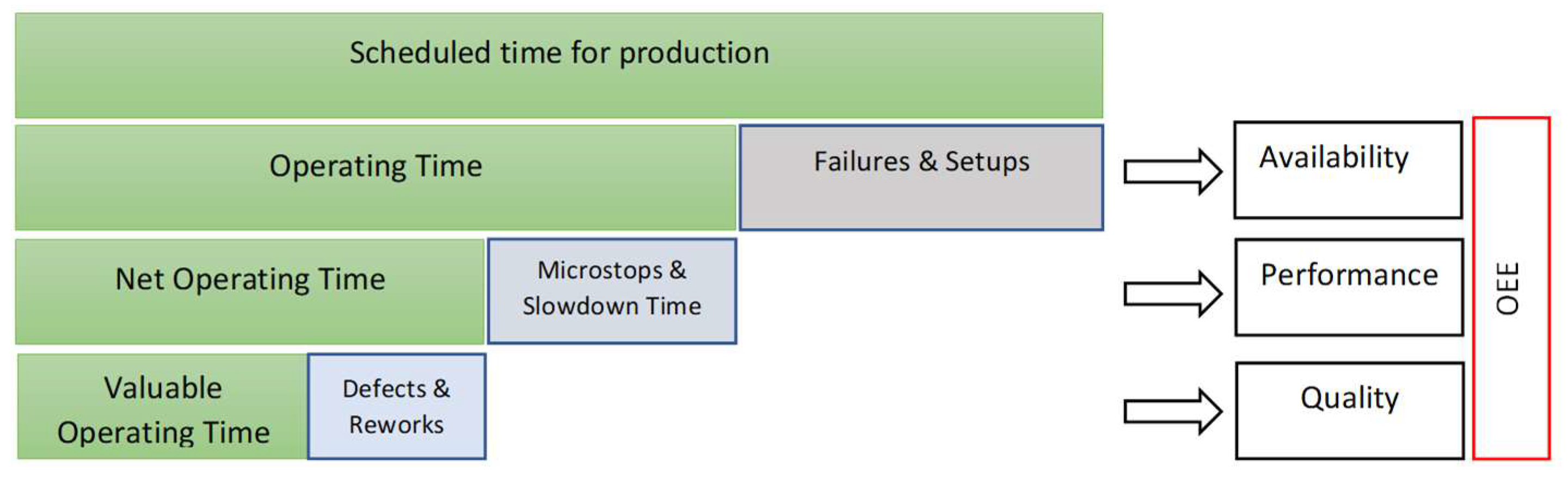
Figure 2.
Characteristics of a warehouse static resource.
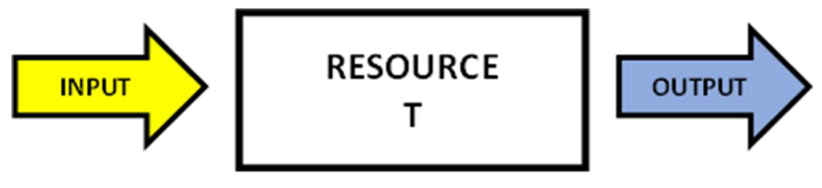
Figure 3.
Representation of OWE in a metric based on output from the warehouse.
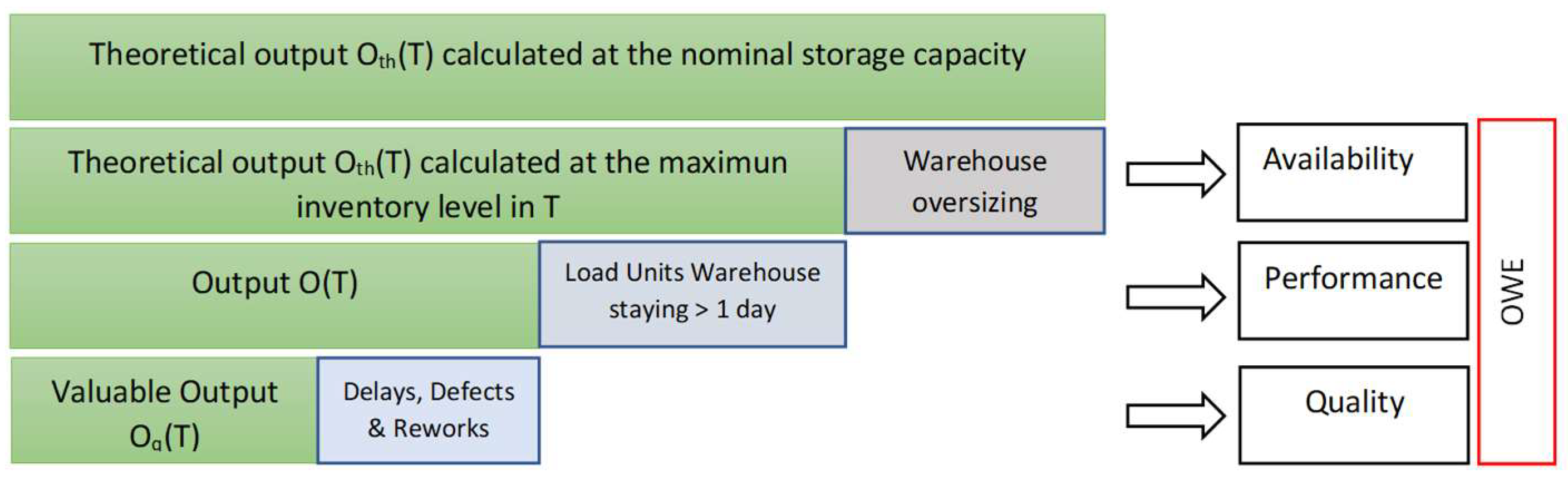
Figure 4.
Input i(t).
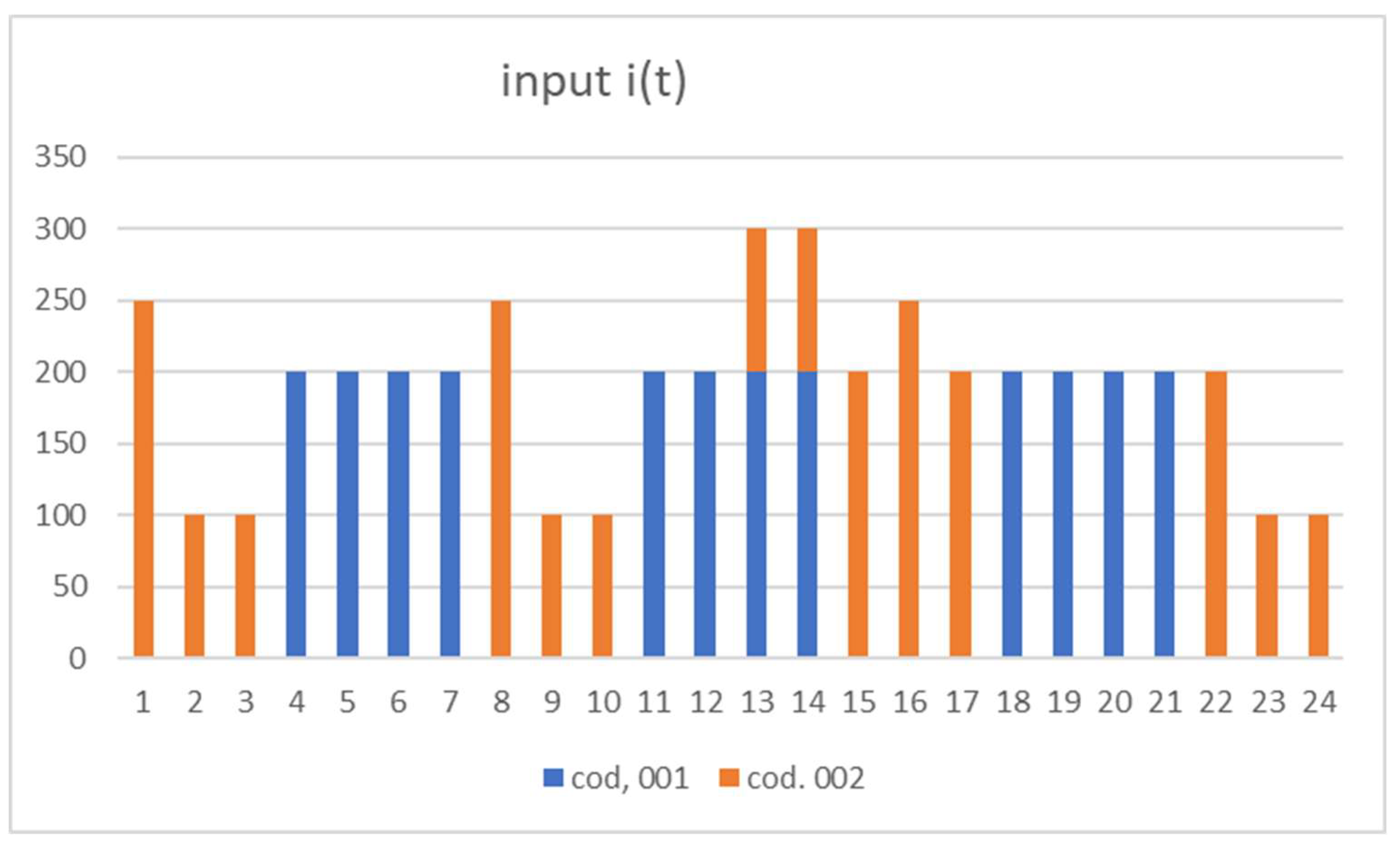
Figure 5.
Output o(t).
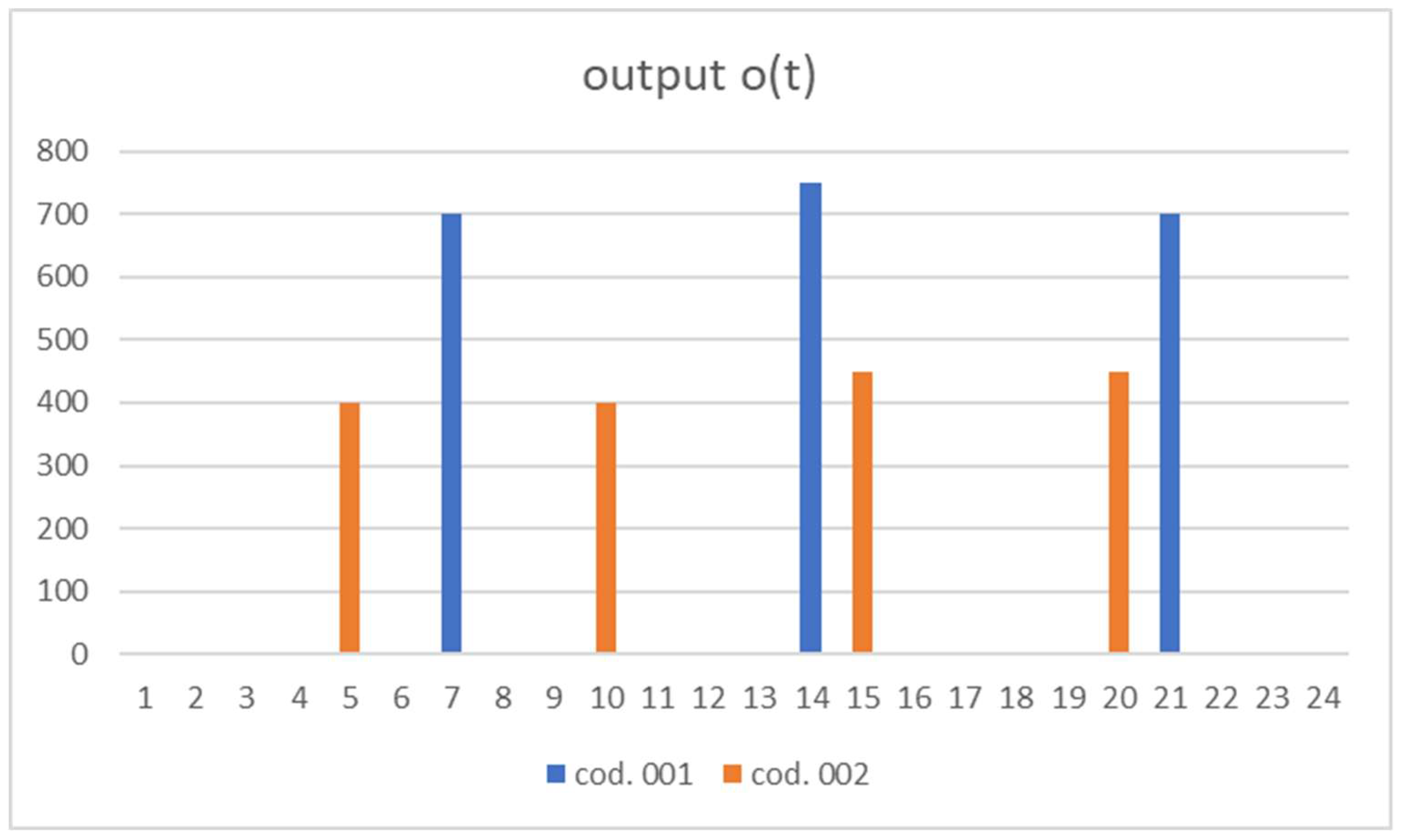
Figure 6.
Output vs. valuable output.
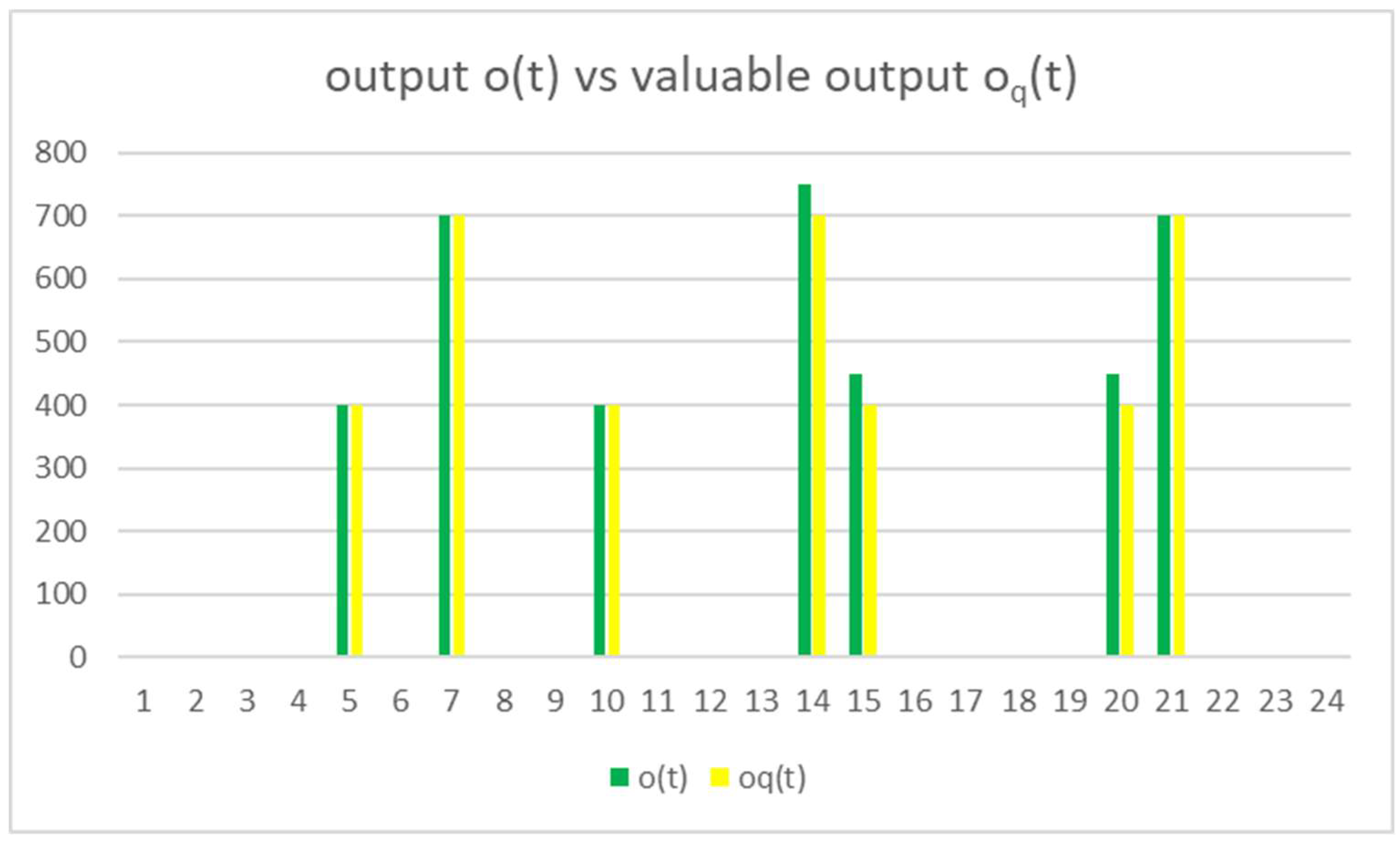
Figure 7.
Inventory Level.
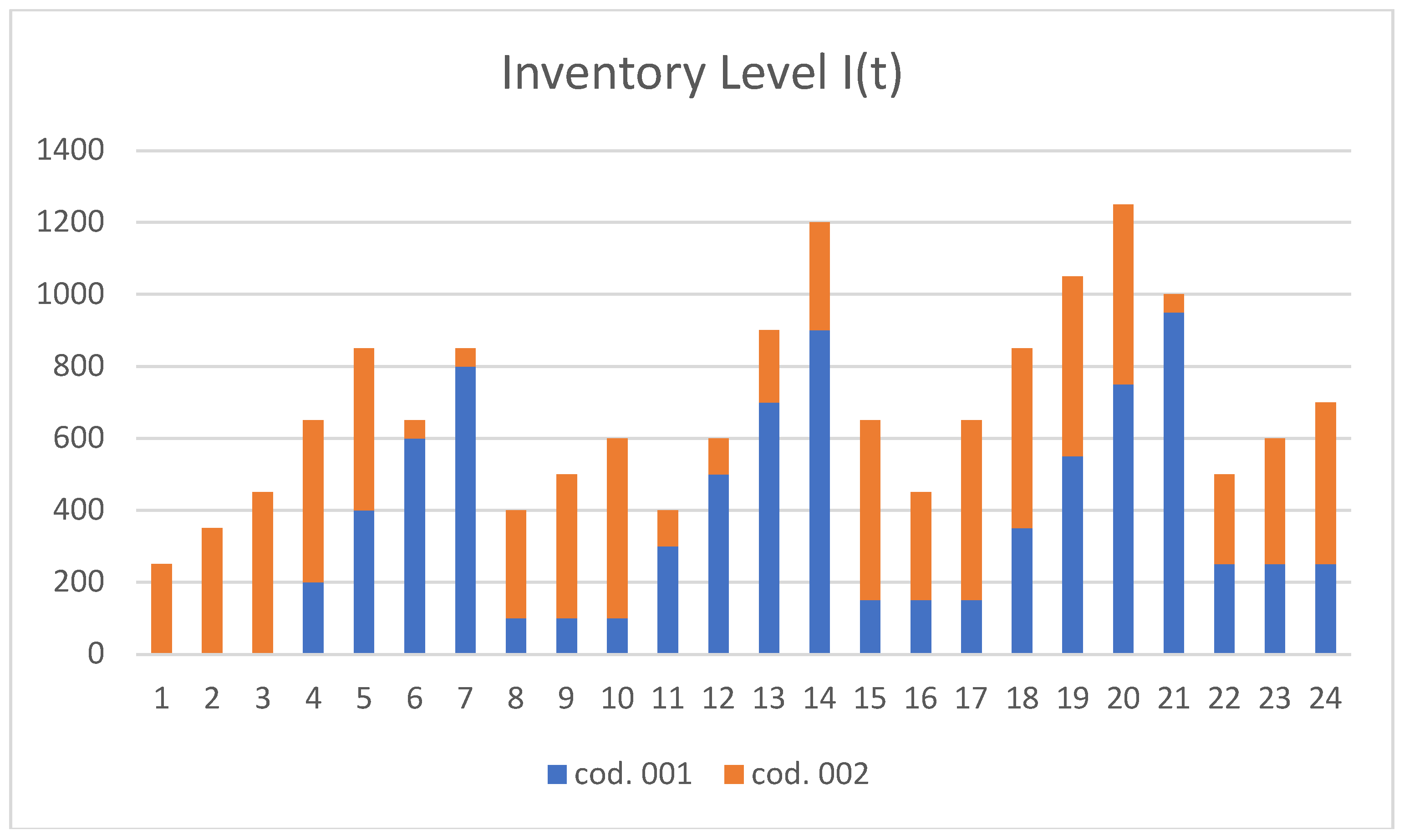
Figure 8.
Standard OWE over a 24 days-period.
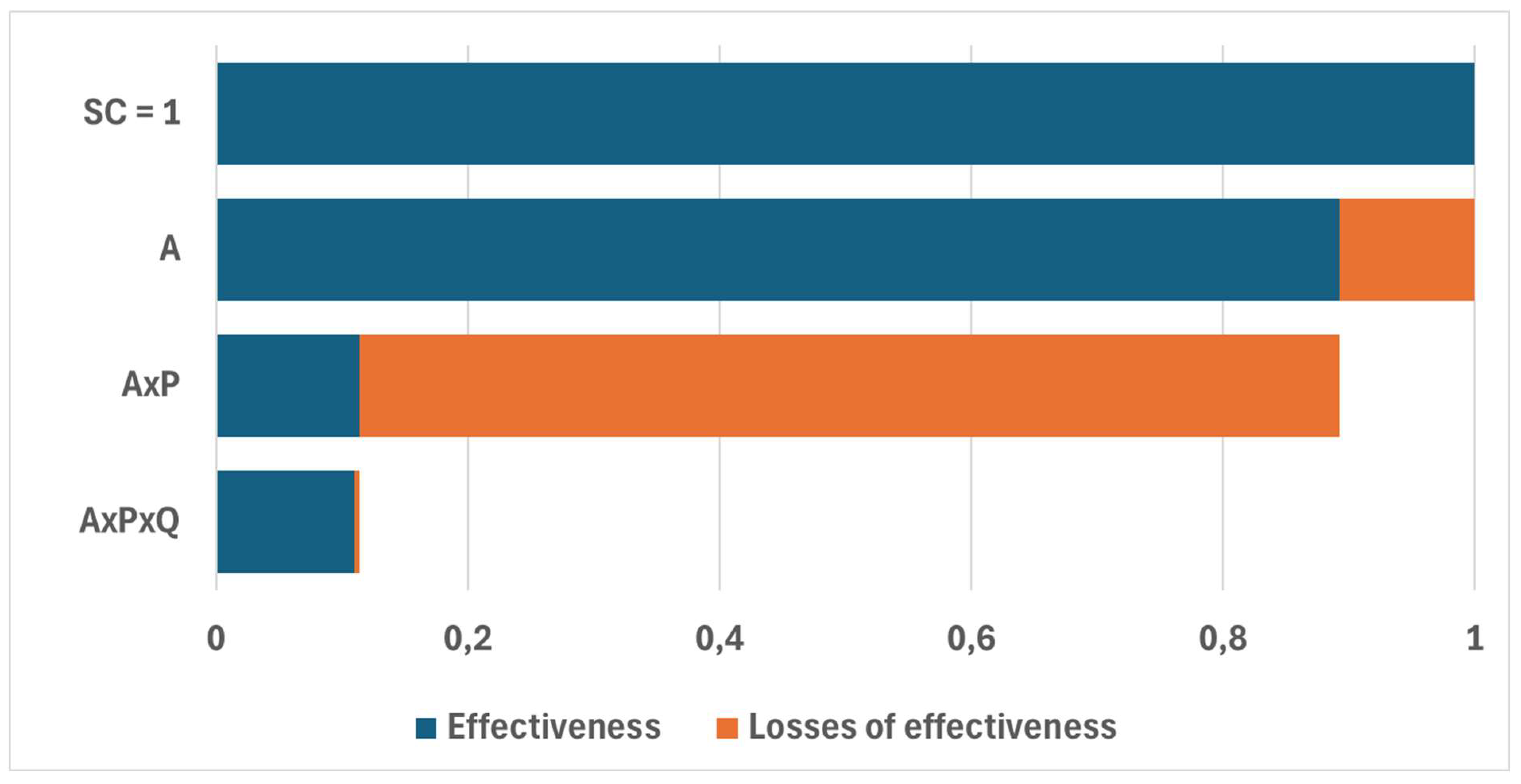
Figure 9.
Output o(t).
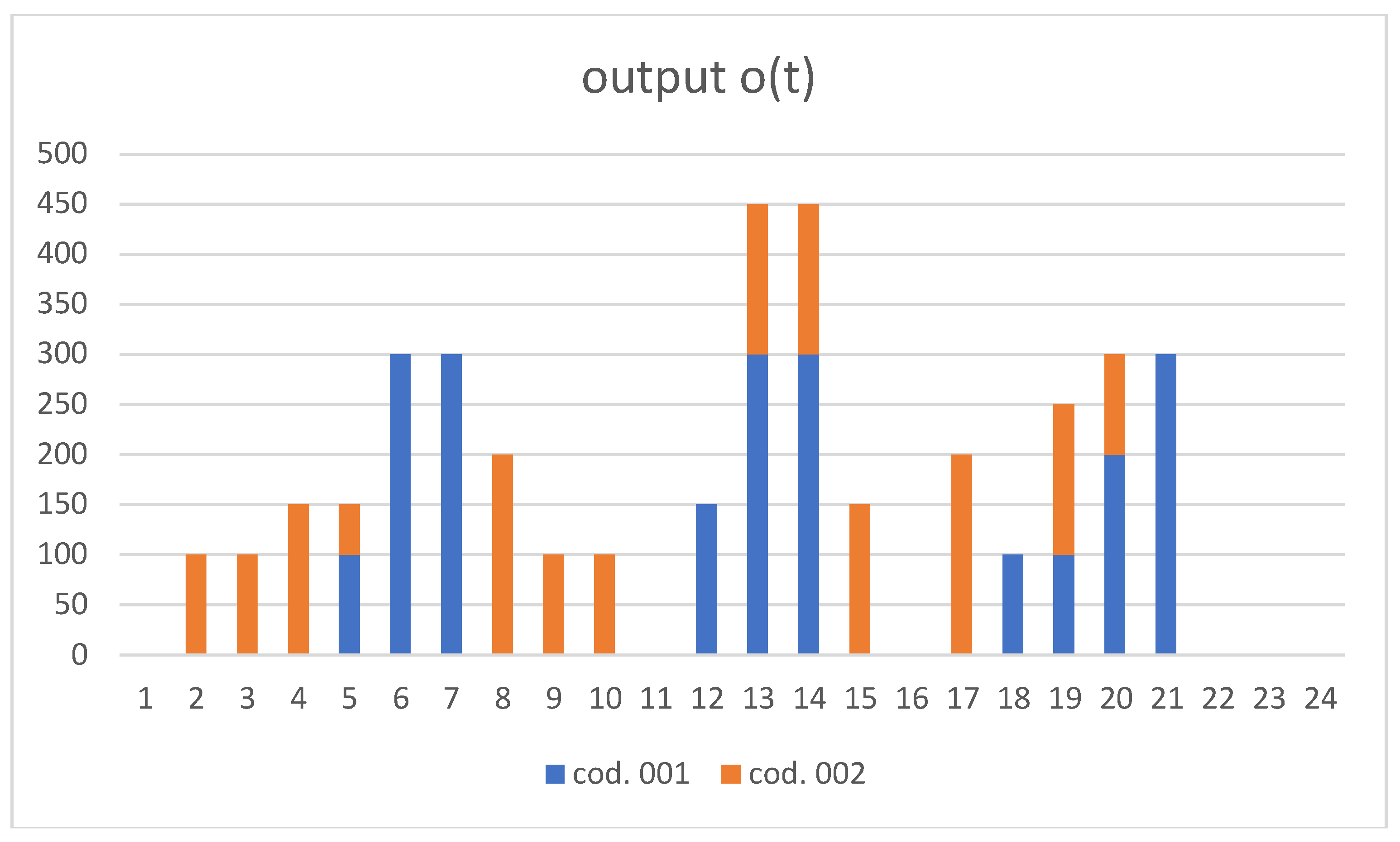
Figure 10.
Output vs. valuable output.
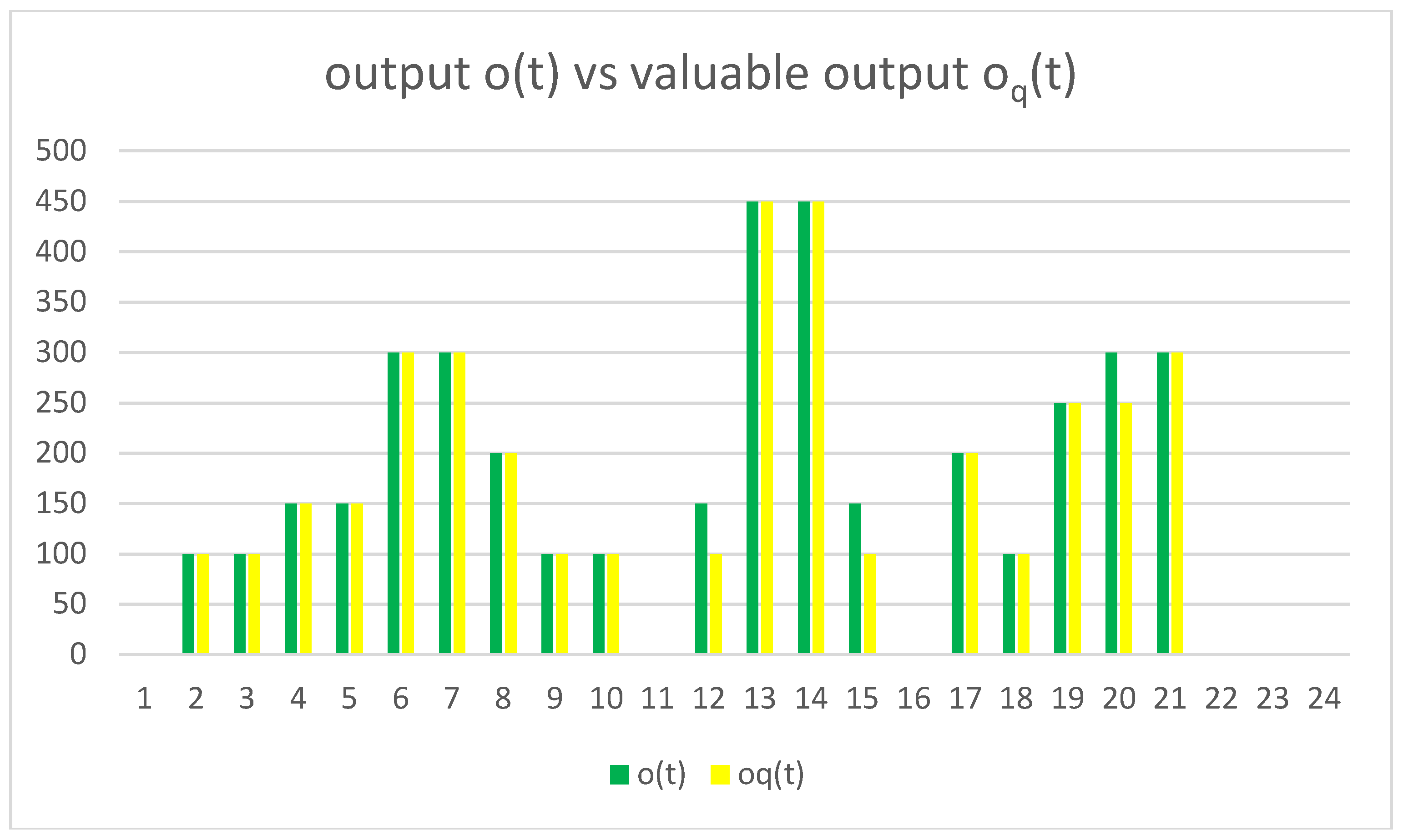
Figure 11.
Inventory Level.
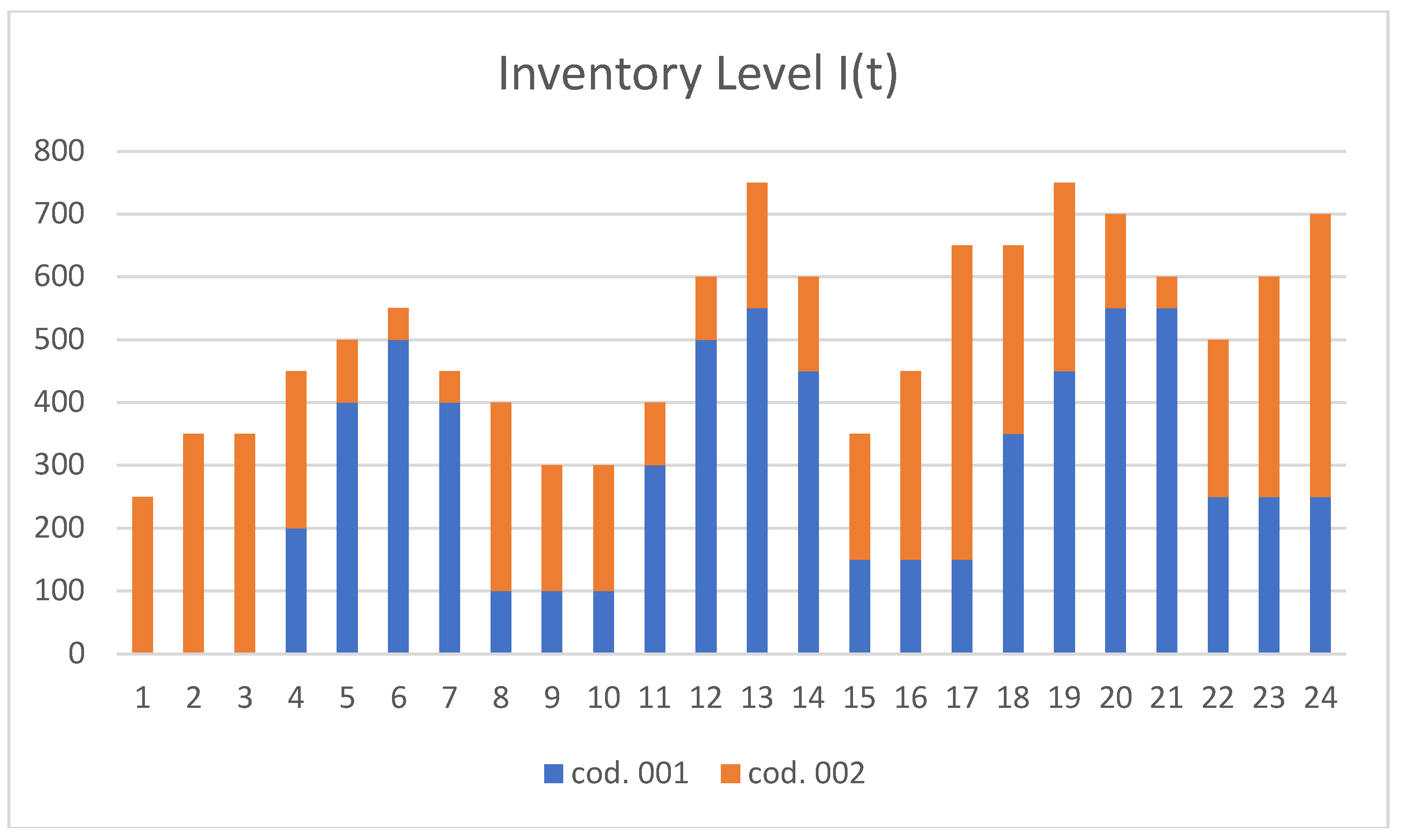

Table 1.
Variations of the OEE in manufacturing contexts.
| Metric | Equation | Variation | Reference |
|---|---|---|---|
| Overall Factory Effectiveness (OFE) | Relationships among different machines and processes | [30] | |
| Overall Asset Effectiveness (OAE) | Losses due to business-related and other non-operationally related causes | [32] | |
| Overall Resources Effectiveness (ORE) | Manufacturing performance measurement system | [31] | |
| Overall Environmental Equipment Effectiveness (OEEE) | Concept of sustainability based on the calculated environmental impact | [35] | |
| Operations Flow Effectiveness (OFE) | Holistic view of material flow through the input-process-output cycles of a firm | [33] | |
| Overall Greenness Performance (OGP) | Environmental hierarchy of metrics according to Va (Value adding) processes | [36] | |
| Overall material usage effectiveness (OME) | Measure the effective material usage within manufacturing processes | [34] | |
| Operations Labour Effectiveness (OLE) | Improvement in safety and fatigue management | [37] |
Table 2.
Comparison of OEE vs. OWE indicators.
| KPI | Availability | Process performance | Quality rate |
|---|---|---|---|
| OEE | Ability of the resource to be actually available to produce compared to the production schedule. (1 bis) |
Actual capacity that the resource can exert to generate value compared to the capacity that is assigned to it in the process design phase. (2 bis) | Ability of the resource to produce compliant parts. (3 bis) |
| OWE | Ability of the resource to be effectively available to maintain goods with respect to the actual planning of input and output flows. | Ability of the resource to maintain assets efficiently and taking into account the actual planning of input and output flows, this ability is expressed by comparison with ideal cases | Ability of the resource to make intact products available to the customer with complete and timely deliveries |
Table 3.
Objective of the OWE indicators referring to the compartment resource.
| OWE parameter | Objective |
|---|---|
| Availability | Warehouse planning allows undersized or oversized warehouses to be identified. It also takes into account the actual availability of compartments. |
| Performance | Effectiveness of stock management policies, taking into account the scheduling of Input and Output flows and stock levels. In addition, it enables to evaluate the different asset allocation criteria from a ‘static’ warehouse point of view. |
| Quality | Congruity of Flow Output with Demand, allows the correct sizing of the operating and safety stock to be verified |
Table 4.
Variables for the mathematical formulations.
| Variable | Definition |
|---|---|
| T | Reference time interval in which the analysis is carried out |
| Storage Capacity (SC) | Storage capacity of the warehouse under analysis, equals the number of available storage locations. |
| Imax(T) | Maximum inventory occurring in the warehouse during the analysis interval T. This value is calculated at the end of T. |
| O(T) | Output or outflow from the warehouse at T, the management of which within the warehouse gives rise to Imax(T). This value is taken at the end of T. |
| Oth,max(T) | The maximum theoretical output or outflow that can be managed in the interval T in a warehouse considering different amount of storage locations occupied. |
Disclaimer/Publisher’s Note: The statements, opinions and data contained in all publications are solely those of the individual author(s) and contributor(s) and not of MDPI and/or the editor(s). MDPI and/or the editor(s) disclaim responsibility for any injury to people or property resulting from any ideas, methods, instructions or products referred to in the content. |
© 2024 by the authors. Licensee MDPI, Basel, Switzerland. This article is an open access article distributed under the terms and conditions of the Creative Commons Attribution (CC BY) license (http://creativecommons.org/licenses/by/4.0/).
Copyright: This open access article is published under a Creative Commons CC BY 4.0 license, which permit the free download, distribution, and reuse, provided that the author and preprint are cited in any reuse.


