
Submitted:
22 November 2024
Posted:
26 November 2024
You are already at the latest version
Abstract
The food industry faces significant challenges in managing operational costs due to its high energy intensity and rising energy prices. Industrial food processing facilities, with substantial thermal capacities and large demands for cooling and heating, offer promising opportunities for demand response (DR) strategies. This study explores the application of deep reinforcement learning (RL) as an innovative, data-driven approach for DR in the food industry. By leveraging the adaptive, self-learning capabilities of RL, energy costs in the investigated plant are effectively decreased. The RL algorithm is compared with the well-established optimization method mixed integer linear programming (MILP), and both are benchmarked against a reference scenario without DR. The two optimization strategies demonstrate cost savings of 17.57% and 18.65% for RL and MILP, respectively. Although RL is slightly less efficient in cost reduction, it significantly outperforms in computational speed, being approximately 20 times faster. During operation, RL only needs 2 ms per optimization compared to 19 s per MILP, making it a promising optimization tool for edge computing. Moreover, while MILP's computation time increases considerably with the number of binary variables, RL efficiently learns dynamic system behavior and scales to more complex systems without significant performance degradation. These results highlight that deep RL, when applied to DR, offers substantial cost savings and computational efficiency, with broad applicability to energy management in various applications.
Keywords:
1. Introduction
1.1. Thermal Capacities for Demand Response
1.2. Reinforcement Learning for Demand Response
1.3. Contributions
- We optimize the set point temperature of a PI controller rather than directly controlling the cooling power. This approach enhances stability and simplifies practical implementation.
- We apply DDQL - a state-of-the-art RL algorithm - for load shifting to reduce energy costs in an RTP scenario.
- We formulate the problem as MILP to compare RL with a state-of-the-art MPC controller.
- We investigate the energy cost savings and the computation time of RL and MILP.
2. Methods
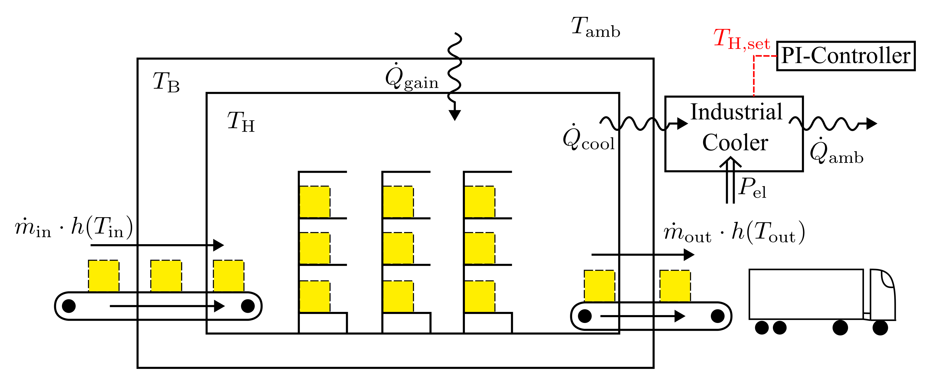
2.1. Industrial Warehouse Model
| Algorithm 1:PI controller with saturation |
|
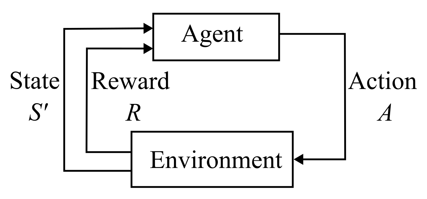
2.2. Reinforcement Learning
| Algorithm 2:Double Deep Q-Learning - Training |
|
2.3. Mixed Integer Linear Programming
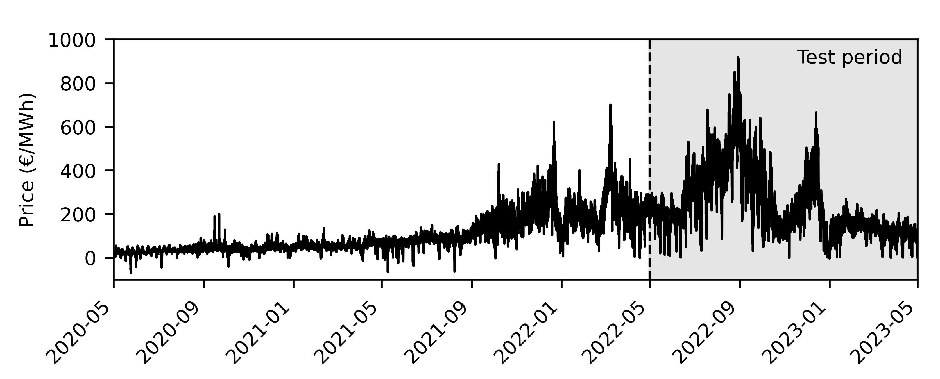
3. Results and Discussion
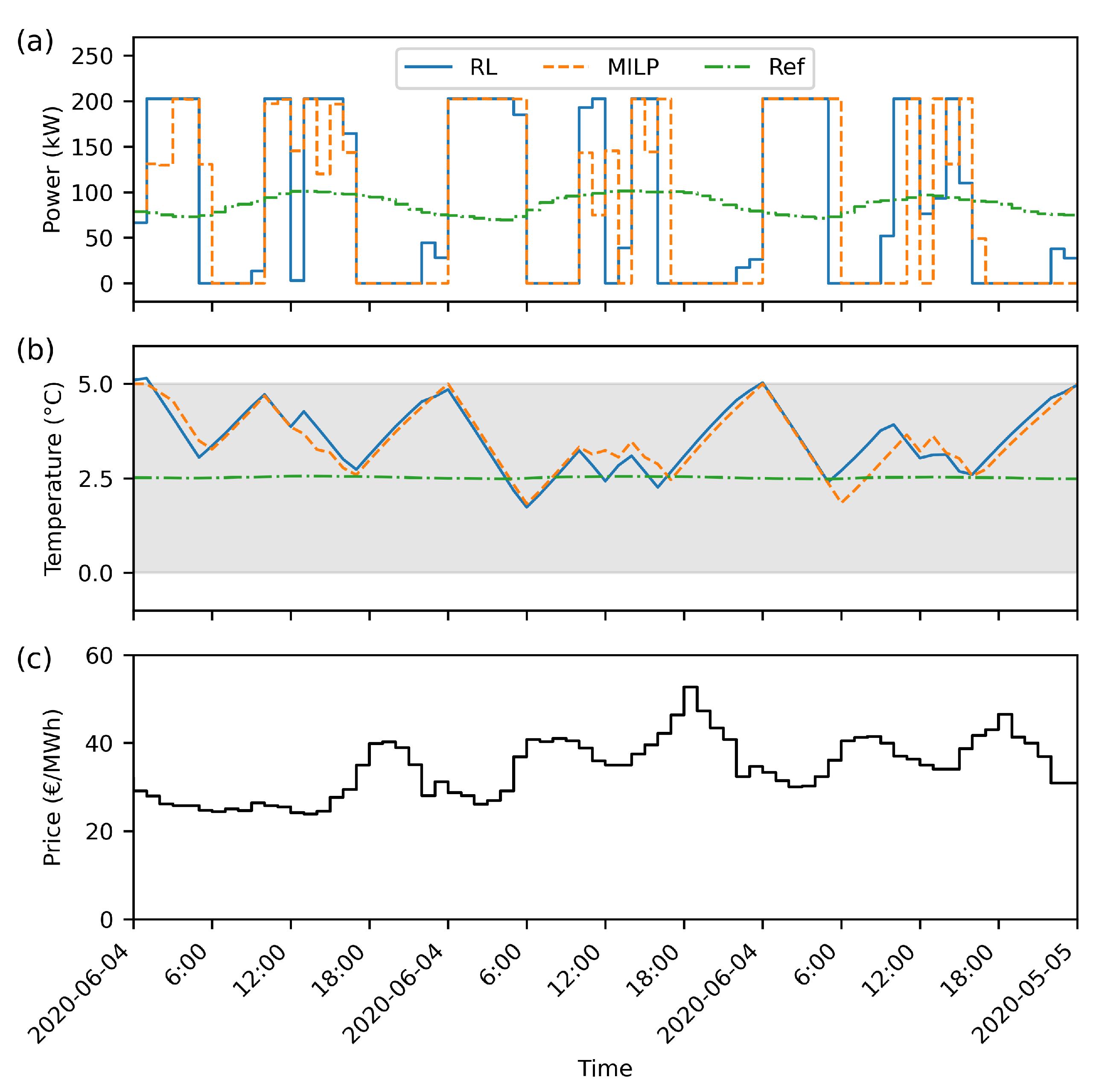
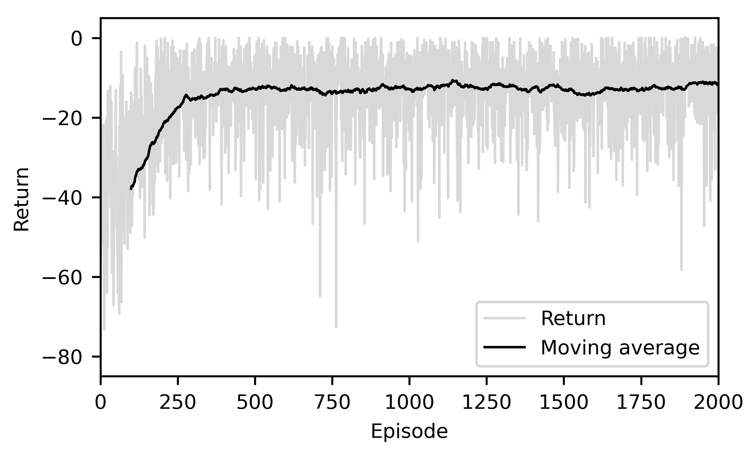
3.1. RL Training Process
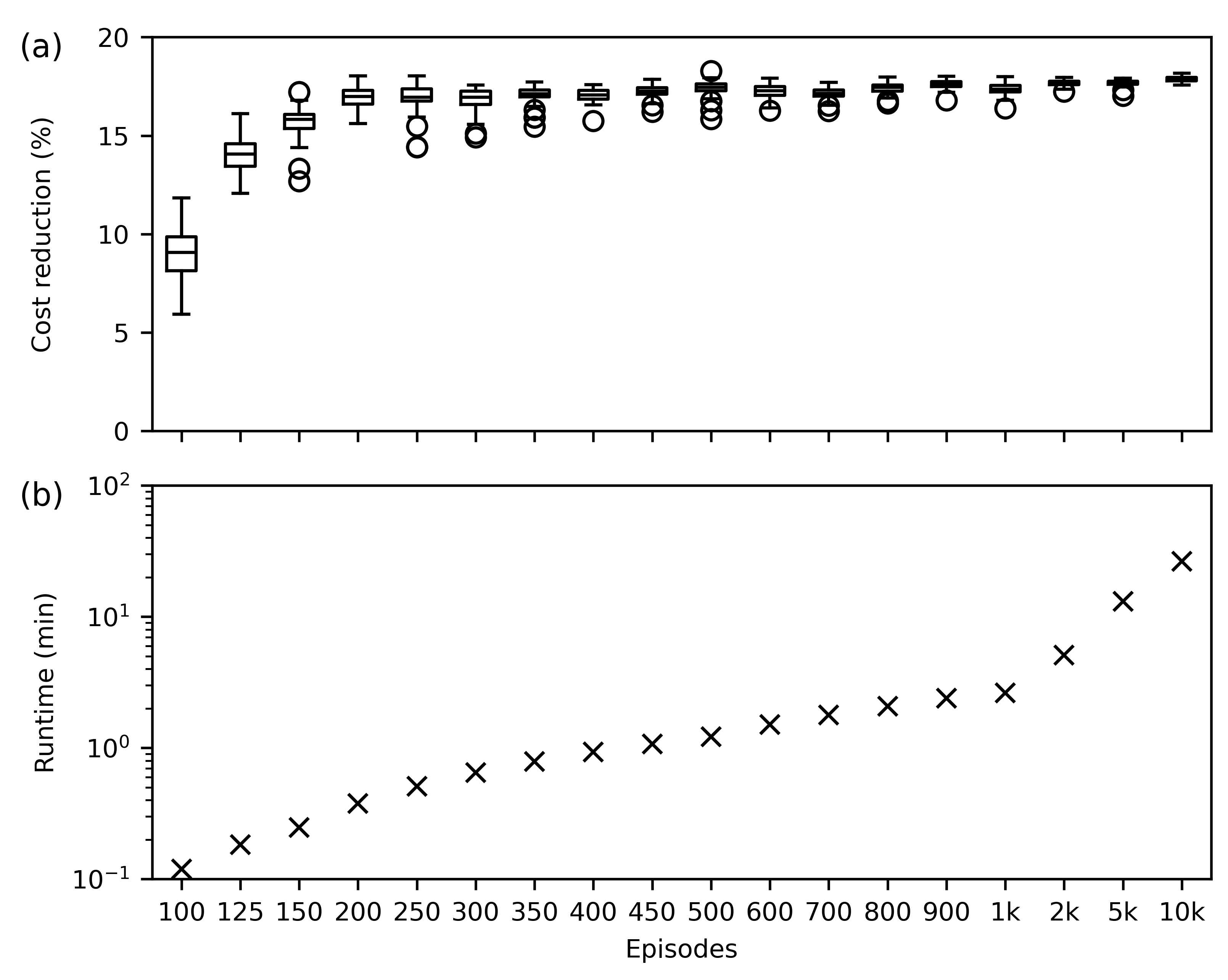
3.2. Computation Time
3.3. Applicability in Practice
4. Conclusions
Author Contributions
Funding
Institutional Review Board Statement
Informed Consent Statement
Data Availability Statement
Acknowledgments
Conflicts of Interest
Abbreviations
| DR | Demand response |
| DDQL | Double deep Q-learning |
| DDPG | Deep deterministic policy gradient |
| DQL | Deep Q-learning |
| DQN | Deep Q-networks |
| DRL | Deep reinforcement learning |
| DSM | Demand side management |
| EXAA | Energy exchange Austria |
| HVAC | Heating, ventilation and air conditioning |
| IoT | Internet of things |
| LP | Linear programming |
| MILP | Mixed integer linear programming |
| MINLP | Mixed integer nonlinear programming |
| ML | Machine learning |
| MPC | Model predictive control |
| PI | Proportional integral |
| PPO | Proximal policy optimization |
| PV | Photovoltaic |
| RL | Reinforcement learning |
| RTP | Real-time pricing |
| SAC | Soft actor-critic |
| TES | Thermal energy storage |
| TOU | Time-of-use |
Appendix A. MILP Formulation
- is the set point temperature of the warehouse during the time period p.
- is the warehouse temperature at the time point t.
- is the output signal of the P-controller before saturation during the time period p.
- is a helper variable to calculate the saturation during the time period p.
- are binary variables to calculate the saturation during the time period p.
- is the electrical power consumption of the industrial refrigeration system p.
- is the price signal during the time period p.
- is the heat flow rate of the load during the time period p.
- is the length of a time period.
- is the initial warehouse temperature at the time point 0.
- is the energy efficiency ratio of the industrial refrigeration system.
- proportional factor of the controller.
- integral factor of the controller.
- is the minimum electrical power.
- is the maximum electrical power.
- is the minimum set point temperature.
- is the maximum set point temperature.
- N is the number of time periods.
- and are big M constraints.
- P is a set for the indices of every time period.
- is a set for the indices of every time point.
- I is a set to index of every hour of a day.
- J is a set to index every minute in a hour.
References
- Gerres, T.; Chaves Ávila, J. P.; Llamas, P. L.; San Román, T. G. A Review of Cross-Sector Decarbonisation Potentials in the European Energy Intensive Industry. Journal of Cleaner Production 2019, 210, 585–601. [Google Scholar] [CrossRef]
- Clairand, J.-M.; Briceno-Leon, M.; Escriva-Escriva, G.; Pantaleo, A. M. Review of Energy Efficiency Technologies in the Food Industry: Trends, Barriers, and Opportunities. IEEE Access 2020, 8, 48015–48029. [Google Scholar] [CrossRef]
- Panda, S.; Mohanty, S.; Rout, P. K.; Sahu, B. K.; Parida, S. ; Samanta, I S. .; Bajaj, M.; Piecha, M.; Blazek, V.; Prokop, L. A comprehensive review on demand side management and market design for renewable energy support and integration. Energy Reports. 2023, 10, 2228–2250. [Google Scholar] [CrossRef]
- Siddiquee, S. M. S.; Howard, B.; Bruton, K.; Brem, A.; O’Sullivan, D. T. J. Progress in Demand Response and It’s Industrial Applications. Frontiers in Energy Research 2021, 9. [Google Scholar] [CrossRef]
- Morais, D.; Gaspar, P. D.; Silva, P. D.; Andrade, L. P.; Nunes, J. Energy Consumption and Efficiency Measures in the Portuguese Food Processing Industry. Journal of Food Processing and Preservation 2022, 46(8), e14862. [Google Scholar] [CrossRef]
- Koohi-Fayegh, S.; Rosen, M. A. A Review of Energy Storage Types, Applications and Recent Developments. Journal of Energy Storage 2020, 27, 101047. [Google Scholar] [CrossRef]
- Brok, N.; Green, T.; Heerup, C.; Oren, S. S.; Madsen, H. Optimal Operation of an Ice-Tank for a Supermarket Refrigeration System. Control Engineering Practice 2022, 119, 104973. [Google Scholar] [CrossRef]
- Hovgaard, T. G.; Larsen, L. F. S.; Edlund, K.; Jørgensen, J. B. Model Predictive Control Technologies for Efficient and Flexible Power Consumption in Refrigeration Systems. Energy 2012, 44(1), 105–116. [Google Scholar] [CrossRef]
- Hovgaard, T. G.; Larsen, L. F. S.; Skovrup, M. J.; Jørgensen, J. B. Optimal Energy Consumption in Refrigeration Systems - Modelling and Non-Convex Optimisation. The Canadian Journal of Chemical Engineering 2012, 90(6), 1426–1433. [Google Scholar] [CrossRef]
- Weerts, H. H. M.; Shafiei, S. E.; Stoustrup, J.; Izadi-Zamanabadi, R. Model-Based Predictive Control Scheme for Cost Optimization and Balancing Services for Supermarket Refrigeration Systems. IFAC Proceedings Volumes 2014, 47(3), 975–980. [Google Scholar] [CrossRef]
- Shafiei, S. E.; Knudsen, T.; Wisniewski, R.; Andersen, P. Data-driven Predictive Direct Load Control of Refrigeration Systems. IET Control Theory & Applications 2015, 9 (7), 1022–1033. [CrossRef]
- Shoreh, M. H.; Siano, P.; Shafie-khah, M.; Loia, V.; Catalão, J. P. S. A Survey of Industrial Applications of Demand Response. Electric Power Systems Research 2016, 141, 31–49. [Google Scholar] [CrossRef]
- Goli, S; Mckane, A; Olsen, D. Demand Response Opportunities in Industrial Refrigerated Warehouses in California. ACEEE Summer Study on Energy Efficiency in Industry (2011) 1–14. Lawrence Berkeley National Laboratory. Retrieved from https://escholarship.
- Akerma, M.; Hoang, H. M.; Leducq, D.; Flinois, C.; Clain, P.; Delahaye, A. Demand Response in Refrigerated Warehouse. In 2018 IEEE International Smart Cities Conference (ISC2); 2018; pp 1–5. [CrossRef]
- Akerma, M.; Hoang, H.-M.; Leducq, D.; Delahaye, A. Experimental Characterization of Demand Response in a Refrigerated Cold Room. International Journal of Refrigeration 2020, 113, 256–265. [Google Scholar] [CrossRef]
- Ma, K.; Hu, G.; Spanos, C. J. A Cooperative Demand Response Scheme Using Punishment Mechanism and Application to Industrial Refrigerated Warehouses. IEEE Transactions on Industrial Informatics 2015, 11(6), 1520–1531. [Google Scholar] [CrossRef]
- Khorsandnejad, E.; Malzahn, R.; Oldenburg, A.-K.; Mittreiter, A.; Doetsch, C. Analysis of Flexibility Potential of a Cold Warehouse with Different Refrigeration Compressors. Energies 2024, 17(1), 85. [Google Scholar] [CrossRef]
- Akerma, M; Hoang, H. M.; Leducq, D; Flinois, C; Clain, P.; Delahaye, A.; Demand response in refrigerated warehouse, 2018 IEEE International Smart Cities Conference (ISC2), Kansas City, MO, USA, 2018, pp. 1-5. [CrossRef]
- Chen, C.; Sun, H.; Shen, X.; Guo, Y.; Guo, Q.; Xia, T. Two-Stage Robust Planning-Operation Co-Optimization of Energy Hub Considering Precise Energy Storage Economic Model. Applied Energy 2019, 252 (C), 1–1. [Google Scholar] [CrossRef]
- Giordano, L.; Furlan, G.; Puglisi, G.; Cancellara, F. A. Optimal Design of a Renewable Energy-Driven Polygeneration System: An Application in the Dairy Industry. Journal of Cleaner Production 2023, 405, 136933. [Google Scholar] [CrossRef]
- Pazmiño-Arias, A.; Briceño-León, M.; Clairand, J.-M.; Serrano-Guerrero, X.; Escrivá-Escrivá, G. Optimal Scheduling of a Dairy Industry Based on Energy Hub Considering Renewable Energy and Ice Storage. Journal of Cleaner Production 2023, 429, 139580. [Google Scholar] [CrossRef]
- Cirocco, L.; Pudney, P.; Riahi, S.; Liddle, R.; Semsarilar, H.; Hudson, J.; Bruno, F. Thermal Energy Storage for Industrial Thermal Loads and Electricity Demand Side Management. Energy Conversion and Management 2022, 270, 116190. [Google Scholar] [CrossRef]
- Saffari, M.; de Gracia, A.; Fernández, C.; Belusko, M.; Boer, D.; Cabeza, L. F. Optimized Demand Side Management (DSM) of Peak Electricity Demand by Coupling Low Temperature Thermal Energy Storage (TES) and Solar PV. Applied Energy 2018, 211, 604–616. [Google Scholar] [CrossRef]
- Wohlgenannt, P.; Huber, G.; Rheinberger, K.; Preißinger, M.; Kepplinger, P. Modelling of a Food Processing Plant for Industrial Demand Side Management. In HEAT POWERED CYCLES 2021 Conference Proceedings, Bilbao, Spain, 10-, pp. 13 April. [CrossRef]
- Wohlgenannt, P.; Huber, G.; Rheinberger, K.; Kolhe, M.; Kepplinger, P. Comparison of Demand Response Strategies Using Active and Passive Thermal Energy Storage in a Food Processing Plant. Energy Reports 2024, 12, 226–236. [Google Scholar] [CrossRef]
- Zhang, Q.; Grossmann, I. E. Enterprise-Wide Optimization for Industrial Demand Side Management: Fundamentals, Advances, and Perspectives. Chemical Engineering Research and Design 2016, 116, 114–131. [Google Scholar] [CrossRef]
- Mnih, V.; Kavukcuoglu, K.; Silver, D.; Rusu, A. A.; Veness, J.; Bellemare, M. G.; Graves, A.; Riedmiller, M.; Fidjeland, A. K.; Ostrovski, G.; Petersen, S.; Beattie, C.; Sadik, A.; Antonoglou, I.; King, H.; Kumaran, D.; Wierstra, D.; Legg, S.; Hassabis, D. Human-Level Control through Deep Reinforcement Learning. Nature 2015, 518(7540), 529–533. [Google Scholar] [CrossRef] [PubMed]
- Watkins, C. J. C. H.; Dayan, P. Q-Learning. Mach Learn 1992, 8(3), 279–292. [Google Scholar] [CrossRef]
- van Hasselt, H. ; Guez, A; Silver, D. In , Deep Reinforcement Learning with Double Q-learning. In Proceedings of the Thirtieth AAAI Conference on Artificial Intelligence (AAAI-16), Phoenix, Arizona, USA, 2094–2100., 12–17 February 2016. [Google Scholar] [CrossRef]
- Vázquez-Canteli, J. R.; Nagy, Z. Reinforcement Learning for Demand Response: A Review of Algorithms and Modeling Techniques. Applied Energy 2019, 235, 1072–1089. [Google Scholar] [CrossRef]
- Yu, L.; Qin, S.; Zhang, M.; Shen, C.; Jiang, T.; Guan, X. A Review of Deep Reinforcement Learning for Smart Building Energy Management. IEEE Internet of Things Journal 2021, 8(15), 12046–12063. [Google Scholar] [CrossRef]
- Lazic, N.; Boutilier, C.; Lu, T.; Wong, E.; Roy, B.; Ryu, M.; Imwalle, G. Data Center Cooling Using Model-Predictive Control. In Advances in Neural Information Processing Systems; Curran Associates, Inc., 2018; Vol. 31. Available online: https://proceedings.neurips.cc/paper/2018/file/ 059fdcd96baeb75112f09fa1dcc740cc- Paper.pdf.
- Part 2: Kinds of RL Algorithms — Spinning Up documentation. Available online: https://spinningup.openai.com/en/latest/spinningup/rl_intro2.html (accessed on day month year).
- Afroosheh, S.; Esapour, K.; Khorram-Nia, R.; Karimi, M. Reinforcement Learning Layout-Based Optimal Energy Management in Smart Home: AI-Based Approach. IET Generation, Transmission & Distribution 2024. [CrossRef]
- Lissa, P.; Deane, C.; Schukat, M.; Seri, F.; Keane, M.; Barrett, E. Deep Reinforcement Learning for Home Energy Management System Control. Energy and AI 2021, 3, 100043. [Google Scholar] [CrossRef]
- Liu, Y.; Zhang, D.; Gooi, H. B. Optimization Strategy Based on Deep Reinforcement Learning for Home Energy Management. CSEE Journal of Power and Energy Systems 2020, 6(3), 572–582. [Google Scholar] [CrossRef]
- Peirelinck, T.; Hermans, C.; Spiessens, F.; Deconinck, G. Double Q-Learning for Demand Response of an Electric Water Heater. In 2019 IEEE PES Innovative Smart Grid Technologies Europe (ISGT-Europe); 2019; pp 1–5. [CrossRef]
- Jiang, Z.; Risbeck, M. J.; Ramamurti, V.; Murugesan, S.; Amores, J.; Zhang, C.; Lee, Y. M.; Drees, K. H. Building HVAC Control with Reinforcement Learning for Reduction of Energy Cost and Demand Charge. Energy and Buildings 2021, 239, 110833. [Google Scholar] [CrossRef]
- Brandi, S.; Piscitelli, M. S.; Martellacci, M.; Capozzoli, A. Deep Reinforcement Learning to Optimise Indoor Temperature Control and Heating Energy Consumption in Buildings. Energy and Buildings 2020, 224, 110225. [Google Scholar] [CrossRef]
- Brandi, S.; Fiorentini, M.; Capozzoli, A. Comparison of Online and Offline Deep Reinforcement Learning with Model Predictive Control for Thermal Energy Management. Automation in Construction 2022, 135, 104128. [Google Scholar] [CrossRef]
- Coraci, D.; Brandi, S.; Capozzoli, A. Effective Pre-Training of a Deep Reinforcement Learning Agent by Means of Long Short-Term Memory Models for Thermal Energy Management in Buildings. Energy Conversion and Management 2023, 291, 117303. [Google Scholar] [CrossRef]
- Han, G.; Lee, S.; Lee, J.; Lee, K.; Bae, J. Deep-Learning- and Reinforcement-Learning-Based Profitable Strategy of a Grid-Level Energy Storage System for the Smart Grid. Journal of Energy Storage 2021, 41, 102868. [Google Scholar] [CrossRef]
- Lu, R.; Hong, S. H. Incentive-Based Demand Response for Smart Grid with Reinforcement Learning and Deep Neural Network. Applied Energy 2019, 236, 937–949. [Google Scholar] [CrossRef]
- Muriithi, G.; Chowdhury, S. Deep Q-Network Application for Optimal Energy Management in a Grid-Tied Solar PV-Battery Microgrid. The Journal of Engineering 2022, 2022(4), 422–441. [Google Scholar] [CrossRef]
- Brandi, S.; Coraci, D.; Borello, D.; Capozzoli, A. Energy Management of a Residential Heating System Through Deep Reinforcement Learning. In Sustainability in Energy and Buildings 2021; Littlewood, J. R., Howlett, R. J., Jain, L. C., Smart Innovation, Systems and Technologies, Eds.; Springer Nature Singapore: Singapore, 2022. [Google Scholar] [CrossRef]
- Brandi, S.; Gallo, A.; Capozzoli, A. A Predictive and Adaptive Control Strategy to Optimize the Management of Integrated Energy Systems in Buildings. Energy Reports 2022, 8, 1550–1567. [Google Scholar] [CrossRef]
- Silvestri, A.; Coraci, D.; Brandi, S.; Capozzoli, A.; Borkowski, E.; Köhler, J.; Wu, D.; Zeilinger, M. N.; Schlueter, A. Real Building Implementation of a Deep Reinforcement Learning Controller to Enhance Energy Efficiency and Indoor Temperature Control. Applied Energy 2024, 368. [Google Scholar] [CrossRef]
- Gao, G.; Li, J.; Wen, Y. DeepComfort: Energy-Efficient Thermal Comfort Control in Buildings Via Reinforcement Learning. IEEE Internet of Things Journal 2020, 7(9), 8472–8484. [Google Scholar] [CrossRef]
- Opalic, S. M.; Palumbo, F.; Goodwin, M.; Jiao, L.; Nielsen, H. K.; Kolhe, M. L. COST-WINNERS: COST Reduction WIth Neural NEtworks-Based Augmented Random Search for Simultaneous Thermal and Electrical Energy Storage Control. Journal of Energy Storage 2023, 72. [Google Scholar] [CrossRef]
- Azuatalam, D.; Lee, W.-L.; de Nijs, F.; Liebman, A. Reinforcement Learning for Whole-Building HVAC Control and Demand Response. Energy and AI 2020, 2, 100020. [Google Scholar] [CrossRef]
- Li, Z.; Sun, Z.; Meng, Q.; Wang, Y.; Li, Y. Reinforcement Learning of Room Temperature Set-Point of Thermal Storage Air-Conditioning System with Demand Response. Energy and Buildings 2022, 259, 111903. [Google Scholar] [CrossRef]
- DAY-AHEAD PREISE. Available online: https://markttransparenz.apg.at/de/markt/Markttransparenz/ Uebertragung/EXAA-Spotmarkt (accessed on day month year).
- Gymnasium Version 0.29.1. Available online: https://pypi.org/project/gymnasium/ (accessed on day month year).
- Lillicrap, T. P.; Hunt, J. J.; Pritzel, A.; Heess, N.; Erez, T.; Tassa, Y.; Silver, D.; Wierstra, D. Continuous Control with Deep Reinforcement Learning. arXiv , 2019. 5 July. [CrossRef]
- Pytorch Version 2.1.1. Available online: https://pytorch.org (accessed on day month year).
- Gurobi Version 11.0. Available online: https://www.gurobi.com (accessed on day month year).

| Parameter | Value |
|---|---|
| 4360MJ/K | |
| 500t | |
| 1260t | |
| 480J/(kg K) | |
| 3270J/(kg K) | |
| 4.938 | |
| 202511W | |
| 0W | |
| 5°C | |
| 0°C | |
| 60s | |
| 500000W/K | |
| 2W/(K s) |
| Parameter | Value |
|---|---|
| Training episodes | 2000 |
| Batch size | 1250 |
| Memory buffer size | 10000 |
| Update rate | 0.005 |
| Adam learning rate | 1e-4 |
| Initial exploration rate | 0.9 |
| End exploration rate | 0.05 |
| Exploration decay rate | 2000 |
| Discount factor | 0.999 |
| Neural net layers | 3 |
| Layer 1 | (50, 256), ReLu activation |
| Layer 2 | (256, 256), ReLu activation |
| Layer 3 | (256, 101), ReLu activation |
| Huber loss parameter | 1 |
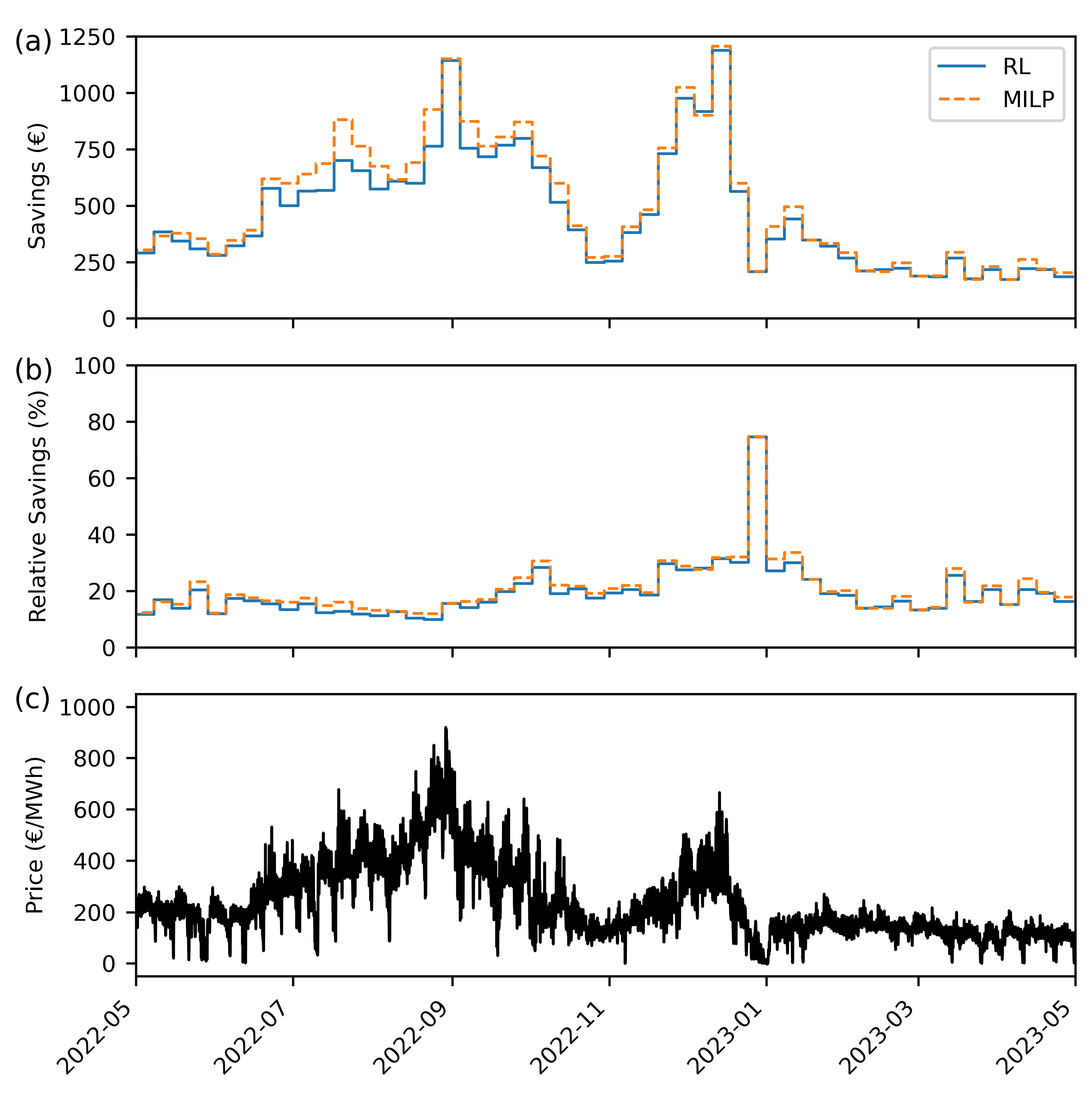
| Optimization | Costs (€) | Savings (€) | Relative savings (%) | Relative costs (€/MWh) |
|---|---|---|---|---|
| RL | 116831 | 24911 | 17.57 | 208.00 |
| MILP | 115301 | 26441 | 18.65 | 205.30 |
| Reference | 141742 | - | - | 252.10 |
Disclaimer/Publisher’s Note: The statements, opinions and data contained in all publications are solely those of the individual author(s) and contributor(s) and not of MDPI and/or the editor(s). MDPI and/or the editor(s) disclaim responsibility for any injury to people or property resulting from any ideas, methods, instructions or products referred to in the content. |
© 2024 by the authors. Licensee MDPI, Basel, Switzerland. This article is an open access article distributed under the terms and conditions of the Creative Commons Attribution (CC BY) license (http://creativecommons.org/licenses/by/4.0/).


