
Submitted:
31 July 2025
Posted:
01 August 2025
You are already at the latest version
Abstract
As energy systems transition toward high shares of variable renewable generation, local energy communities (ECs) are increasingly relevant for enabling demand-side flexibility and self-sufficiency. This shift is particularly evident in the residential sector, where the deployment of photovoltaic (PV) systems is rapidly growing. While mixed-integer linear programming (MILP) remains the standard for operational optimization and demand response in such systems, its computational burden limits scalability and responsiveness under real-time or uncertain conditions. Reinforcement learning (RL), by contrast, offers a model-free, adaptive alternative. However, its application to real-world energy system operation remains limited. This study explores the application of a Deep Q-Network to a real residential EC, which has received limited attention in prior work. The system comprises three single-family homes sharing a centralized heating system with a thermal energy storage (TES), a PV installation, and grid connection. We compare the performance of MILP and RL controllers across economic and environmental metrics. Relative to a reference scenario without TES, MILP and RL reduce energy costs by 10.06% and 8.75%, respectively, and both approaches yield lower total energy consumption and CO2-equivalent emissions. Notably, the trained RL agent achieves a near-optimal outcome while requiring only 22% of the MILP’s computation time. These results demonstrate that Double Deep Q-Learning can offer a computationally efficient and practically viable alternative to MILP for real-time control in residential energy systems.
Keywords:
multi-energy optimization
; energy community
; net zero-energy building
; reinforcement learning
; mixed integer linear programming
; double deep Q-learning
1. Introduction
As modern energy systems become increasingly dominated by renewable, variable power generation, local energy communities (ECs) emerge as a promising way to stabilize the grid and utilize electricity where it is generated [1]. These advantages foster the transition from individual buildings toward Net Zero Energy Buildings [2] or even a Net Zero Energy Neighborhood [3,4]. For the optimization and ideal operation of such systems, Mixed-Integer Linear Programming (MILP) has been regarded as the gold standard for many years. MILP is a powerful method for finding global optima, making it widely used in model-based optimization across economics, logistics, and energy-related fields [5,6,7]. However, as the complexity of the investigated systems increases, the required linearizations become more intricate, and computation times grow exponentially due to the introduction of additional binary variables. This prompts the need for alternative techniques [8]. Recent advances in machine learning and computational power have renewed interest in alternative methods for optimization and control. Reinforcement learning (RL), being model-free and data-driven, significantly reduces computation time once an agent has been trained, while still being able to approach the optimal solutions found using MILP [9,10]. However, since reinforcement learning (RL) is data-driven, agents require a sufficient amount of high-quality data for training. Consequently, training time becomes a critical factor in real-world applications, especially as retraining may be necessary during deployment. And while model-based approaches do not depend on historical data, RL agents tend to outperform traditional methods in the optimization process due to their faster execution and greater computational efficiency once trained. In ECs, where distributed flexibilities can be aggregated and coordinated across multiple entities, RL-based optimization approaches present a promising solution. Due to their decentralized and dynamic nature, such systems benefit from RL agents’ ability to support real-time decision-making under uncertainty. Ideally, this leads to reduced costs for all participants [11]. Optimizing single households often requires transparency and a willingness to compromise on comfort, as optimal control may lead to small temperature variations or limited availability during unforeseen events. Neighborhood-level solutions can help mitigate these issues, as aggregation typically leads to a smoother load curve in larger systems [12,13,14]. In the following subsection, relevant publications on applications of MILP and RL optimization in different energy systems are critically discussed.
1.1. Related Works
In several studies on energy systems, MILP optimization has been investigated and compared to a rule-based conventional operation. Baumann et al. [15] used a co-simulation approach of IDA ICE and Gurobi to optimize the energy system’s control. The building was then optimized on a daily basis using MILP and simulated using a physical resistor-capacitor (RC) model. The investigation demonstrated significant benefits including reduced electricity costs, improved self-consumption and self-sufficiency. In the work of Aguilera et al. [16], MILP was used to control large-scale heat pumps in a simulation utilizing thermal demand forecasts as well as heat pump performance maps. This optimization achieved cost savings in the operation using the digital twin model. Kepplinger et al. [17] also applied the MILP approach in a simulation, incorporating forecasting and state estimation methods to optimally control a heating element in a domestic hot water heater. In their later work, they validated their results using an experimental real-world setup [18]. Cosic et al. [19] extended the application of MILP optimization from operational scheduling to investment planning. In a comprehensive framework, they optimized the sizing and placement of PV and storage systems in a real Austrian municipality, evaluating multiple tariff and market scenarios to demonstrate the model’s adaptability and precision. A 15% reduction in total energy costs and a 34% reduction in emissions was achieved.
RL has also been utilized as an optimizing method for energy systems, although primarily using incentive functions not related to economics. Bachseitz et al. [20] investigated various RL algorithms in comparison to a rule-based control strategy for managing the heat pump of a multi-family building. Their findings indicate that while the RL agent was able to maintain the required storage temperatures, it fell short of matching the rule-based approach in maximizing PV self-consumption. Lissa et al. [21] implemented an RL agent guided by a reward structure based on comfort levels and energy consumption to manage the energy system of a simulated single-family home. They achieved energy savings of 8 % as well as an increased use of renewable energy compared to a rule-based approach. Rohrer et al. [22] applied RL in a lab experiment to evaluate its feasibility for demand response. Using six months of real-world data for training, their approach achieved considerable energy savings, once more emphasizing the practical potential of RL in real demand response scenarios. Franzoso et al. [23] highlighted the use of reinforcement learning to optimize multi-energy systems integrating renewable technologies. Their study demonstrated improved energy management by reducing emissions as well as operational costs, showing the versatility of RL in energy applications.
Langer and Völling investigated a system comprising a single-family home with a heat pump, PV system, and battery electric storage system, optimized using an RL approach [24]. Their RL solution achieved a performance close to the results of a MILP model developed in their earlier work [25]. The evaluation focused on user comfort, grid feed-in, and overall energy usage, but did not account for economic incentives. While this demonstrates the feasibility of RL for residential energy management, the absence of cost considerations limits its applicability in scenarios where financial optimization is critical.
While MILP and RL have been widely studied for building-level energy optimization, few works compare both methods in a comprehensive manner and using real-world data from an existing neighborhood energy system. Furthermore, most RL studies focus on comfort or energy savings, often ignoring economic incentives driven by real-time electricity prices. Finally, the leveraging of price signals and the flexibility of storage, while accounting for PV production, remains insufficiently explored at the community scale. These gaps are addressed in the present study by directly comparing MILP and RL for economic optimization of an EC using historical real-time pricing and measured on-site data. The detailed contributions of this work are described in the following subsection.
1.2. Contribution
This study comprehensively compares RL and MILP side by side under closely matched conditions using both measured and synthetic data for an existing EC, including demand, real-time electricity prices and PV generation profiles. The optimization focuses on exploiting the flexibility of an existing thermal energy storage (TES) by shifting the heat pump operation toward periods of low electricity prices while avoiding high-price intervals, thereby reducing overall energy costs. To enable a thorough comparison of the optimization methods, a reference scenario without flexibility was used, where heat demand is met directly. The individual contributions of this study are:
- Side-by-side comparison of MILP and RL, for the economic optimization of an existing EC using real-world input data and real-time electricity prices.
- Development of an RL-based control strategy for economic demand response, leveraging price signals to shift grid usage toward low-price periods by optimizing the operation of thermal storage and PV flexibility, aiming to approach the MILP-derived optimum.
- Comprehensive benchmark of RL and MILP optimization in a direct comparison and compared to a no-flexibility reference scenario. Within the benchmark cost savings, operational strategies, and robustness under realistic conditions, including PV variability and demand patterns, are assessed.
Therefore, this study provides practical insights into the performance and trade-offs of RL and MILP in energy system optimization, paving the way towards future control strategies for cost-efficient operation of ECs.
2. Methods
In this section, the system is presented and the used methods are highlighted, from general equations over the RL implementation and the MILP.
2.1. System
A real-world energy system was investigated in this study. The small EC, as illustrated in Figure 1, comprises three single-family homes that share both electrical and thermal energy infrastructure. The electrical side includes a grid connection point and rooftop photovoltaic panels. The thermal energy system is centered around a sensible TES, providing flexibility to the two heat-supply components: a 12 kW geothermal heat pump (HP) serving as the primary heat source, and a 6 kW auxiliary resistance heating element (HE) to cover peak loads. The storage tank has a capacity of 1120 liters of water and operates between 35°C and 55°C (), allowing for approximately 26 kWh of storage capacity ().
The direction of the energy flows is indicated by arrows in Figure 1. All flows labeled with the letter P represent electrical power exchanged between system components. These include solar power generation (), the general electrical load of the homes (), and the electrical power consumption of the heating components, the heat pump () and the heating element (). All of these flows are unidirectional, with the exception of the grid connection (), which can either source electricity from the grid () or feed in surplus electricity generated by the PV system ().
Thermal energy flows, denoted by , indicate the direction of heat transfer between components. The heat generated by the heat pump () and the heating element () is stored in the TES. While the majority of the stored energy is ultimately used to meet the EC’s heating demand (), heat losses to the environment () must also be taken into account. It is noteworthy that in the investigated real energy system, a bypass option to directly cover the heating demand using the heat pump and/or heating element is not available. While the heat load from the TES supplies the required energy for space heating, domestic hot water consumption is accounted for within the synthetically generated electric load profile .
2.2. Data
The data used for the simulation and optimization of the EC is categorized as real-world (measured) on-site data, historical data, or synthetic data, as summarized in Table 1.
Measured data were logged for a period of one year from October 19, 2022. The sensors recorded data at a one-minute resolution, which were averaged and stored every 15 minutes, resulting in 96 samples per day and a total of samples for the entire year. The synthetic data was generated with the same temporal resolution to ensure consistency across all datasets. Historical data was resampled to this resolution when necessary.
The measured temperature data exhibited considerable noise due to the interference from the heat pump operation especially when used for cooling the buildings in the summer period, resulting in large fluctuations of the measured ground probe temperature profile. To ensure smooth simulation and optimization, as well as realistic COP and power estimates for both optimization methods, the data was preprocessed prior to any algorithmic use. Namely, a rolling average filter for 96 values was applied to smoothen the signal, resulting in a synthetic signal derived from the measured signal.
For the RL optimization, the seasonal classification was considered by assigning binary values to each time step, where a value of 1 indicates the active season. Seasons were defined as shown in Table 2.
For validation and to ensure robustness of the algorithms, a train-test split was applied to the data, as seen in Figure 2. This split was designed to include all seasons and their combinations within both sets. Specifically, the data for each month were divided such that in total 260 of the days were used for training and the remaining 105 for testing. The exception was the initial month, October 2022, which was exclusively allocated to training, and the final month, October 2023, exclusively to testing. This approach ensures comprehensive seasonal coverage during both training and testing phases.
2.3. Physical Model
The EC was modeled through a series of equations to calculate the used energy and energy flows at each timestep. For this model, the following assumptions were made:
- The specific heat capacity of water is equal to , irrespective of the TES temperature.
- Spatial temperature variations in the TES are neglected, making it a single node model.
- The mass balance is always fulfilled for the TES. Due to the narrow operating temperature range of only 20 °C, the volume of the storage is assumed to remain constant, as thermal expansion effects are negligible.
- The electric power of the heating element is equivalent to its heating power ().
- The COP of the heat pump is equal to . This is in accordance with Walden and Pedulla [32].
The heat capacity of the sensible water storage was calculated using the volume of the tank , the specific density of water , and the specific heat capacity of water :
Using the specific heat capacity and the temporal change of temperature of the storage tank at each timestep, the change in stored energy can be calculated. This was done by accounting for the heat flows to and from the tank, namely the heat supplied by the heating element , the heat pump , the heating demand , and the heat losses :
To calculate the heating power of the heating element, the electrical power input and the efficiency of the system are required:
The heating power of the heat pump, denoted as , was computed based on its electrical input power and an estimated coefficient of performance (COP) at each timestep. To this end, the ideal Carnot COP was used to model the temperature dependency of the heat pump COP, which depends on the heat sink temperature and the ground probe temperature .
For simplification, the heating demand was defined as the total heat consumption of the three separate houses in the energy system, , , and . These individual demands were aggregated into a single total demand:
The heat losses of the storage tank were calculated using the heat transfer coefficient h, the total surface area of the tank A, and the temperature difference between the storage temperature and the ambient temperature :
Using the previously defined heat capacity (see Equation (1)), the temporal rate of change of the storage tank temperature can also be expressed by:
Alternatively, assuming constant heat fluxes and parameters over time, the storage temperature evolution can be analytically described by the solution of the first-order linear differential equation:
The heating power was controlled using a simple, discrete-time proportional P-controller with saturation, as shown in Algo. A1. At each time step i, with a duration of , the control error was computed as the difference between the desired storage temperature and the actual temperature . The heating power was then calculated by multiplying this error with the proportional gain . To ensure that the power remains within operational limits, was constrained to lie within the range defined by and . The heating element was set to activate if the temperature of the TES drops to 2 degrees below , acting strictly as an auxiliary heating unit. Both the RL and the MILP optimization are able to freely adjust the set temperature in order to utilize the flexibility of the thermal storage system. This flexibility is determined by the thermal capacity and the temperature bounds and , set to 35°C and 55°C, respectively.
A state of charge (SOC) was defined for the TES, and it is computed based on the storage temperature at time t according to:
where is the current storage temperature, and and denote the upper and lower temperature bounds of the storage system.
The remaining parameters were derived from system documentation and planning materials. The complete energy system model was used as the environment for the RL agent, which was implemented using Python and the Gymnasium framework [33], and pytorch [34]. The MILP model was formulated and solved using the Gurobipy interface to the Gurobi optimizer [35]. Both models rely on the parameters listed in Table 3.
2.4. Reinforcement Learning
This subsection outlines the deep reinforcement learning (RL) algorithm employed to the control of the heat pump and the heating element to reduce the energy costs and improve the self consumption. A Deep Q-Network (DQN) was implemented, following the approach presented in our earlier work [36]. The architecture of the DQN is illustrated in Figure 3.
The method builds upon the deep Q-learning algorithm originally introduced by Mnih et al. [37], and incorporates key improvements proposed by Van Hasselt et al. [38], which involve using two separate neural networks: a policy network for selecting actions and a target network for estimating Q-values. To enhance training stability, the algorithm integrates soft target updates as described by Lillicrap et al. [39]. Additionally, it uses experience replay with mini-batch sampling, following the stabilization technique as applied in the original DQN study [37].
In the present EC, the heating system’s controller acts as the agent, controlling the heat generators HP and HE, while the rest of the EC acts as the environment based on external conditions and actions. The agent’s control action consists of adjusting the SOC of the TES. The action set is discretized on a scale from 0 to 100, where 0 represents the minimum allowable TES charge and 100 the maximum, as regulated by the P-controller.
The optimization horizon covers one day, partitioned into 96 discrete time steps of h each. Consequently, one episode spans 96 steps. The system state at each step i is composed of the current (scaled between 0 and 100), the number of remaining steps in the day, the forecasted electricity prices for the upcoming 96 intervals, the feed-in tariff f, the predicted thermal output , the net electrical loads , and the seasonal indicator variables for those intervals. The forecasts for electricity prices and thermal load are assumed available one day in advance, reflecting realistic operational conditions where day-ahead market prices are published prior to execution. For the purposes of this application, operation is assumed to occur under perfect predictions without uncertainty, thereby simplifying the optimization problem. After each step, the forecast window shifts forward accordingly; unknown future values beyond the forecast horizon are set to zero. To enhance training stability, most state variables are scaled.
Electricity prices, used in calculating energy costs and rewards, were scaled according to a min-max normalization over the course of one day to a range from 1 to 10 via:
Similarly, the feed-in tariff f, which remains constant throughout each episode, was scaled using the same minimum and maximum values as the electricity prices to ensure consistent normalization:
Scaling electricity prices serves three main purposes: first, it ensures that all state variables have comparable magnitudes; second, it normalizes daily price values to account for seasonal fluctuations; and third, it enables the agent to generalize to price scenarios that differ from those seen during training. Importantly, scaled prices were constrained to be greater than or equal to one, which avoids zero-cost intervals that might otherwise encourage unrealistic energy usage.
Thermal loads are scaled to represent the percentage of the TES capacity consumed per time step:
where is the thermal capacity of the TES.
To keep the state vector as small as possible, the electrical load and PV generation have been summarized in the singular net load :
Collectively, the state vector at time step i is given by:
The discrete action space from 0 to 100 corresponds to the target SOC () for the P controller, from which the temperature setpoint is computed as:
The environment dynamics were modeled using Equation (9) alongside a P-controller. Although each episode consists of 96 discrete time steps representing a full day, the P controller operates at a higher frequency within each simulation step, executing 60 control updates per time interval. The scaled price signal was then incorporated into the reward function, which distinguishes between grid consumption and feed-in:
where and denote the electrical powers, consumed or fed in the grid, respectively, the denotes the scaled electricity price at step i and f the constant feed-in tariff.
The hyperparameters of the RL algorithm are summarized in Table A1. The following steps were taken for training the RL agent:
- At the start of each episode, a day index was randomly sampled from the training dataset.
- For the selected day, the corresponding normalized profiles were loaded, including electricity prices , thermal load demand , electrical load , and feed-in tariffs .
- Seasonal indicators such as winter (), spring (), summer (), and autumn () flags were extracted for the selected day. This approach ensures diversity across episodes and captures a wide range of operational conditions.
- The agent was trained over a total of episodes.
2.5. Mixed Integer Linear Programming
In this section, the MILP model is introduced and described. The system was modeled and optimized to determine the global optimum of the EC’s operation. In order to ensure a fair comparison with the RL approach, the MILP model was provided with perfect prediction for each day of operation. This includes complete knowledge of the overall heat demand , electricity prices , feed-in tariffs f, ground probe temperatures , and photovoltaic generation . The optimization was carried out over a horizon of discrete time stamps, resulting in 96 time periods p between them as , covering one full day.
The parameters used for the MILP formulation correspond to Table 3. The objective function minimizes the net electricity cost by considering the grid import power (), the electricity price signal , the feed-in power (), and the feed-in tariff f, as well as the number of time steps N. The objective function is formulated as:
This objective was calculated with a fixed horizon of 24 hours, more precisely defined as 96 quarter-hour intervals. Since each day was optimized independently and the total cost was calculated at the end, the following temperature bounds for were considered for consistency:
As seen in the equations, the first day was initialized with a storage temperature of 40°C. On all following days, except the last one, the optimization began with the final temperature of the previous day, i.e., , to ensure that no energy is artificially lost or gained. While the optimizer was allowed to chose the end-of-day temperature of each day freely, on the last day the final storage temperature was fixed to to maintain consistency with the RL.
All other constraints of the model are listed below and must be satisfied at every timestep on each day. These include operational limits, system dynamics, and technical constraints, all of which ensure the physical and economic feasibility of the optimization results across the full time horizon.
All variables used are bound by their respective boundaries as follows:
As already mentioned in the description of the reinforcement learning approach, the 96 values forecasted for the electricity price , feed-in tariffs f, overall heat demand , electrical load , and solar generation were assumed to be perfectly accurate under the assumption of perfect prediction. This assumption simplifies the optimization by neglecting forecasting errors, allowing the model to focus solely on the system’s operational optimization. However, in practical applications, forecasting uncertainties do impact the solution quality and must be considered for a more robust approach.
3. Results and Discussion
In this section, the results of both optimizers are presented and discussed. In Figure 4, various electric energy flows P within the system are presented. Panel a displays five days of electrical power flows under the RL-optimized operation, while panel c shows the behavior of the MILP-based system. Power flows into the hub, including photovoltaic generation () and grid import (), are represented as positive values. In contrast, power flows leaving the hub, such as the electrical load (), the heat pump (), the heating element (), and electricity exported to the grid as feed-in (), are represented as negative values. The corresponding real-time electricity price signal and the constant feed-in tariff are shown in panel b.
Although the general operation patterns appear similar at first glance, several key differences emerge between the two control strategies, most notably in the operation of the auxiliary heating element. For the heating element, the RL agent tends to favor longer periods of moderate operation or to avoid its activation altogether. In contrast, the MILP model opts for short, high-intensity bursts, operating the auxiliary heater at full capacity when required. This indicates a more aggressive but shorter-duration heating strategy under the MILP control to achieve the global optimum of operation. Both optimization approaches clearly attempt to maximize the self-consumption of PV-generated electricity before feeding into the grid. The constant feed-in tariff of 0.08 €/kWh appears insufficient to incentivize export when local usage is possible. Furthermore, the five-day excerpt illustrates a period of high thermal demand. Both systems frequently operate the heat pump and auxiliary heating elements at or near their maximum power levels, indicating a substantial heating demand driven by cold weather conditions (below -4°C) for the EC. These conditions correspond to the second percentile of all annually occurring ambient temperatures.
Figure 5 depicts the transient energy balance of the TES depicted as a time-series for the same time period as depicted in Figure 4. It showcases the RL-controlled and the MILP-controlled operations, panel a and panel c, respectively. Positive flows symbolize heat entering the sensible storage tank during the operation of the heating element or the heat pump; negative flows therefore depict the heat taken from the TES, i.e., the heating load for space heating. The sum of the heat flows is depicted as and reflects the charging power (or discharging power, if negative) of the TES within a period. In panel b, the temperatures of both operation modes are shown in degrees centigrade as well as in % SOC.
Starting with the temperature curves in b, the general shapes are quite similar, indicating a similar approach by both RL and MILP. The main difference between the two is that RL manages to dip under the lower temperature constraint, which prompts the logic of the RL to activate the heating element. As the MILP is bound by the temperature constraints, it is not allowed to let this happen. For the general operation seen in a and b, the approach seems quite similar, as both systems have the same heat load applied to them. For these five days, the RL seems to have a more bipolar behavior, not using the inverter function of the heat pump, but instead turning it on and off, while the MILP operation seems to utilize the modulation ability of the heat pump, resulting a more continuous and moderated operation of the storage tank, while the RL-optimized TES exhibits more frequent and abrupt switching between charging and discharging.
To compare the performance of the reference scenario with the RL and MILP optimization approaches, five key performance indicators (KPIs) were selected, as illustrated in Figure 6. Panel a presents the relative deviation of both optimization methods from the reference case in terms of cumulative costs, eq emissions, grid power consumption, self-consumption ratio (SCR), and self-sufficiency ratio (SSR). In addition to these relative deviations, Table 4 provides the corresponding absolute values. Panel b displays the cumulative cost evolution over the 105-day testing period, highlighting the comparative behavior of the MILP and RL approaches.
As seen in panel a, MILP and RL are generally quite similar in their results. Both optimizers achieve cost savings compared to the reference scenario. While the MILP is able to find the global optimum at 10.06% reduction compared to the reference scenario, the RL optimization is able to approach this with 8.75%. Although not optimizing for emissions, emissions are also reduced in the RL and MILP case, by 4.94% and 4.01%, respectively. Grid power usage is nearly the same irrespective of the optimization strategy. One reason why emissions could be reduced is the increase in the SCRs and SSRs. As solar power was considered as -neutral, an increase in self-consumption leads to a reduction in . This also explains the better results of the RL optimization, as it achieved the highest self-consumption rate, thereby also reducing emissions.
The cumulative cost curves in panel b reveal that the overall shape remains similar across both optimization approaches and the reference scenario. However, starting in spring, the curves begin to diverge as the optimized strategies achieve increasing cost savings. This divergence is driven by two opposing trends: higher PV production yields more energy that can be used directly, while milder temperatures reduce the heating load and thus the overall energy demand . Over the full year, MILP and RL achieve total savings of 67.58 € and 58.76 €, respectively, with MILP delivering the best overall result and RL performing comparably close.
4. Conclusions
This study shows that optimization algorithms like RL can approach the global optimum as determined via MILP to a degree where the difference is negligible in practice. Based on the measured KPIs, RL even outperforms MILP in some areas, including CO2, SCR, and SSR, making it a strong candidate for real-world applications. This study distinguishes itself by using high-resolution, real-world data, including measured demand, PV generation, and real-time electricity prices, under near-identical conditions for both methods.
Even if the result is promising and the optimization itself is faster in RL than it is for MILP, there are some aspects to consider. RL has two main downsides. First, a large amount of data is needed to train and validate the agent, which even required the implementation of additional features such as seasonality or normalized data. Secondly, training for episodes took multiple hours to complete, meaning that from point zero to optimization, MILP was much faster than RL, the reason being the multidimensional state of each training episode combined with the relatively fine temporal resolution of 15-minute steps. Another topic which cannot be discounted is the implementation of the auxiliary heating element in the RL. The kind of implementation used allows the RL-optimized system to drop below the hard lower bounds of the MILP by two degrees before applying the heating element, leading to some temperature violations, which gives RL slightly more flexibility overall. However, a closer inspection shows that these violations are generally mild, with only 1 % of cases falling below 34.0°C and none below 33.0°C.
Despite these limitations, RL demonstrates strong performance under realistic conditions. With some targeted preprocessing, it is able to achieve near-optimal results and offers the key advantage of real-time control once training is complete. In deployment, the agent can act autonomously and adapt over time through retraining or transfer learning, making RL a promising solution for dynamic environments and potentially suitable for edge applications. Both approaches should be able to improve the performance of a simple system, so the question might not always be which method can produce the better result, but rather which method is more feasible for real-world application, as small and fast computers become increasingly available.
Future research could focus on validating these findings in real-world settings, for example through lab setups using synthetic loads. Expanding the system to include additional components like solar thermal, biomass combined heat and power, or decentralized storage would test both scalability and robustness. Another valuable direction is the integration of real load forecasting and resilience to unexpected events such as sudden demand shifts or system faults. Beyond the immediate results, this work contributes to a growing body of evidence that learning-based control strategies can approach traditional optimization methods under certain real-world constraints. The insights gained from this study can be applied to similar energy systems and extended to other flexibility assets, supporting the transition from academic methods to real-world deployment.
Ultimately, this work delivers one of the first direct, high-resolution comparisons of RL and MILP for optimizing an existing EC using real-world data, PV generation, and market signals. It demonstrates that deep RL is not only a viable alternative to MILP but can in some cases even match a carefully tuned MILP model, while offering practical advantages in speed, adaptability, and scalability for real-time control of complex energy systems.
Acknowledgments
The authors gratefully acknowledge the financial support from the Austrian Research Promotion Agency FFG for the Hub4FlECs project (COIN FFG 898053). The authors also gratefully acknowledge the support by Ludwig Netzer from Netzer Group providing real-world data.
Appendix A. Additional Configurations
| Algorithm A1 P-controller with saturation and auxiliary heater logic |
|

Table A1.
RL Parameters.
| Parameter | Value |
|---|---|
| Training episodes | 5000 |
| Batch size | 1250 |
| Memory buffer size | 10,000 |
| Update rate | 0.005 |
| Adam learning rate | |
| Initial exploration rate | 0.9 |
| End exploration rate | 0.05 |
| Exploration decay rate | 5000 |
| Discount factor | 0.999 |
| Neural network layers | 3 |
| Layer 1 | (input, 512), ReLU activation |
| Layer 2 | (512, 512), ReLU activation |
| Layer 3 | (512, 101), linear activation |
| Loss function | Huber Loss |
References
- Seiler, V.; Moosbrugger, L.; Huber, G.; Kepplinger, P. Assessing Model Predictive Control for Energy Communities’ Flexibilities. In Proceedings of the Intelligente Energie- und Klimastrategien: Energie – Gebäude – Umwelt, Forschung / Forschungszentrum Energie, Wien, 2024; Vol. 30, Science.Research.Pannonia, pp. 1–22. Conference publication; peer-reviewed; Open Access; CC BY 4.0. [CrossRef]
- Jaysawal, R.K.; Chakraborty, S.; Elangovan, D.; Padmanaban, S. Concept of net zero energy buildings (NZEB) - A literature review. Cleaner Engineering and Technology 2022, 11, 100582. [Google Scholar] [CrossRef]
- Riechel, R. Zwischen Gebäude und Gesamtstadt: Das Quartier als Handlungsraum in der lokalen Wärmewende. Vierteljahrshefte zur Wirtschaftsforschung 2016, 85, 89–101. [Google Scholar] [CrossRef]
- Kannengießer, T. Bewertung zukünftiger urbaner Energieversorgungskonzepte für Quartiere. PhD thesis, Rheinisch-Westfälische Technische Hochschule Aachen, 2023. Dissertation zur Erlangung des akademischen Grades eines Doktors der Ingenieurwissenschaften.
- Ren, H.; Gao, W. A MILP model for integrated plan and evaluation of distributed energy systems. Applied Energy 2010, 87, 1001–1014. [Google Scholar] [CrossRef]
- Lindholm, O.; Weiss, R.; Hasan, A.; Pettersson, F.; Shemeikka, J. A MILP Optimization Method for Building Seasonal Energy Storage: A Case Study for a Reversible Solid Oxide Cell and Hydrogen Storage System. Buildings 2020, 10. [Google Scholar] [CrossRef]
- Wohlgenannt, P.; Huber, G.; Rheinberger, K.; Kolhe, M.; Kepplinger, P. Comparison of demand response strategies using active and passive thermal energy storage in a food processing plant. Energy Reports 2024, 12, 226–236. [Google Scholar] [CrossRef]
- Urbanucci, L. Limits and potentials of Mixed Integer Linear Programming methods for optimization of polygeneration energy systems. Energy Procedia 2018, 148, 1199–1205, ATI 2018 - 73rd Conference of the Italian Thermal Machines Engineering Association. [Google Scholar] [CrossRef]
- Vázquez-Canteli, J.R.; Nagy, Z. Reinforcement learning for demand response: A review of algorithms and modeling techniques. Applied Energy 2019, 235, 1072–1089. [Google Scholar] [CrossRef]
- Wang, Z.; Hong, T. Reinforcement learning for building controls: The opportunities and challenges. Applied Energy 2020, 269, 115036. [Google Scholar] [CrossRef]
- Charbonnier, F.; Peng, B.; Vienne, J.; Stai, E.; Morstyn, T.; McCulloch, M. Centralised rehearsal of decentralised cooperation: Multi-agent reinforcement learning for the scalable coordination of residential energy flexibility. Applied Energy 2025, 377, 124406. [Google Scholar] [CrossRef]
- Palma, G.; Guiducci, L.; Stentati, M.; Rizzo, A.; Paoletti, S. Reinforcement Learning for Energy Community Management: A European-Scale Study. Energies 2024, 17. [Google Scholar] [CrossRef]
- Guiducci, L.; Palma, G.; Stentati, M.; Rizzo, A.; Paoletti, S. A Reinforcement Learning Approach to the Management of Renewable Energy Communities. In Proceedings of the 2023 12th Mediterranean Conference on Embedded Computing (MECO); 2023; pp. 1–8. [Google Scholar] [CrossRef]
- Pereira, H.; Gomes, L.; Vale, Z. Peer-to-peer energy trading optimization in energy communities using multi-agent deep reinforcement learning. Energy Informatics 2022, 5, 44. [Google Scholar] [CrossRef]
- Baumann, C.; Wohlgenannt, P.; Streicher, W.; Kepplinger, P. Optimizing heat pump control in an NZEB via model predictive control and building simulation. Energies 2025, 18. Jg. [Google Scholar] [CrossRef]
- Aguilera, J.J.; Padullés, R.; Meesenburg, W.; Markussen, W.B.; Zühlsdorf, B.; Elmegaard, B. Operation optimization in large-scale heat pump systems: A scheduling framework integrating digital twin modelling, demand forecasting, and MILP. Applied Energy 2024, 376, 124259. [Google Scholar] [CrossRef]
- Kepplinger, P.; Huber, G.; Petrasch, J. Autonomous optimal control for demand side management with resistive domestic hot water heaters using linear optimization. Energy and Buildings 2015, 100, 50–55. [Google Scholar] [CrossRef]
- Kepplinger, P.; Huber, G.; Petrasch, J. Field testing of demand side management via autonomous optimal control of a domestic hot water heater. Energy and Buildings 2016, 127, 730–735. [Google Scholar] [CrossRef]
- Cosic, A.; Stadler, M.; Mansoor, M.; Zellinger, M. Mixed-integer linear programming based optimization strategies for renewable energy communities. Energy 2021, 237, 121559. [Google Scholar] [CrossRef]
- Bachseitz, M.; Sheryar, M.; Schmitt, D.; Summ, T.; Trinkl, C.; Zörner, W. PV-Optimized Heat Pump Control in Multi-Family Buildings Using a Reinforcement Learning Approach. Energies 2024, 17, 1908. [Google Scholar] [CrossRef]
- Lissa, P.; Deane, C.; Schukat, M.; Seri, F.; Keane, M.; Barrett, E. Deep reinforcement learning for home energy management system control. Energy and AI 2021, 3, 100043. [Google Scholar] [CrossRef]
- Rohrer, T.; Frison, L.; Kaupenjohann, L.; Scharf, K.; Hergenröther, E. Deep Reinforcement Learning for Heat Pump Control. arXiv 2022. [Google Scholar] [CrossRef]
- Franzoso, A.; Fambri, G.; Badami, M. Deep reinforcement learning as a tool for the analysis and optimization of energy flows in multi-energy systems. Energy Conversion and Management 2025, 341, 120095. [Google Scholar] [CrossRef]
- Langer, L.; Volling, T. A reinforcement learning approach to home energy management for modulating heat pumps and photovoltaic systems. Applied Energy 2022, 327, 120020. [Google Scholar] [CrossRef]
- Langer, L.; Volling, T. An optimal home energy management system for modulating heat pumps and photovoltaic systems. Applied Energy 2020, 278, 115661. [Google Scholar] [CrossRef]
- EXAA Energy Exchange Austria. Spot Market Prices for Austria: 19.10.2022 – 19.10.2023. https://markt.apg.at/transparenz/uebertragung/day-ahead-preise/, 2023. Hourly spot electricity prices from EXAA for the Austrian market covering the period 19 October 2022 to 19 October 2023.
- illwerke vkw, AG. PV-Einspeisetarife Vorarlberg 2025, 2024.
- Ökostrom-Einspeisetarifverordnung 2018 (ÖSET-VO 2018). Bundesgesetzblatt für die Republik Österreich, 2018. BGBl. II Nr. 408/2017, § 6.
- Electricity Maps. Austria 19.10.2022 – 19.10.2023 Carbon Intensity Data (Version January 27, 2025). https://www.electricitymaps.com, 2025. Accessed on: 2025-07-22.
- GGV Stadtwerke Groß-Gerau Versorgungs GmbH. Standard Load Profiles (SLP) — File: GGV_SLP_1000_MWh_2021_01.xlsx. https://www.ggv-energie.de/cms/netz/allgemeine-daten/netzbilanzierung-download-aller-profile.php, 2021. Standard load profile data provided by GGV Stadtwerke Groß-Gerau. File version: 2020-09-24.
- GeoSphere Austria. Messstationen Stundendaten v2 — ID 1115 Feldkirch Global Radiation Data (10-Minute Resolution), 2024. [CrossRef]
- Walden, J.V.; Padullés, R. An analytical solution to optimal heat pump integration. Energy Conversion and Management 2024, 320, 118983. [Google Scholar] [CrossRef]
- Towers, M.; Kwiatkowski, A.; Terry, J.; Balis, J.U.; Cola, G.D.; Deleu, T.; Goulão, M.; Kallinteris, A.; Krimmel, M.; KG, A.; et al. Gymnasium: A Standard Interface for Reinforcement Learning Environments. arXiv 2024. [Google Scholar] [CrossRef]
- Paszke, A.; Gross, S.; Massa, F.; Lerer, A.; Bradbury, J.; Chanan, G.; Killeen, T.; Lin, Z.; Gimelshein, N.; Antiga, L.; et al. PyTorch: An Imperative Style, High-Performance Deep Learning Library. In Proceedings of the Advances in Neural Information Processing Systems 32 (NeurIPS 2019). Curran Associates, Inc. 2019; pp. 8024–29. [Google Scholar]
- Gurobi Optimization, LLC. Gurobi Optimizer Reference Manual, 2025.
- Wohlgenannt, P.; Hegenbart, S.; Eder, E.; Kolhe, M.; Kepplinger, P. Energy Demand Response in a Food-Processing Plant: A Deep Reinforcement Learning Approach. Energies 2024, 17, 6430. [Google Scholar] [CrossRef]
- Mnih, V.; Kavukcuoglu, K.; Silver, D.; Rusu, A.A.; Veness, J.; Bellemare, M.G.; Graves, A.; Riedmiller, M.; Fidjeland, A.K.; Ostrovski, G.; et al. Human-level control through deep reinforcement learning. Nature 2015, 518, 529–533, Publisher: Nature Publishing Group. [Google Scholar] [CrossRef]
- van Hasselt, H.; Guez, A.; Silver, D. Deep Reinforcement Learning with Double Q-learning. arXiv 2015, arXiv:1509.06461. [Google Scholar] [CrossRef]
- Lillicrap, T.P.; Hunt, J.J.; Pritzel, A.; Heess, N.; Erez, T.; Tassa, Y.; Silver, D.; Wierstra, D. Continuous control with deep reinforcement learning. arXiv 2019, arXiv:1509.02971. [Google Scholar]
Figure 1.
Schematic of the energy system, including electrical components (grid and PV), as well as thermal components such as the heat pump, the heating element, and the thermal storage tank. Arrows indicate the direction of energy flows. Flows labeled P denote electrical power: solar generation (), household load (), heat pump (), heating element (), and grid exchange (). Flows labeled denote heating power: heat pump (), heating element (), heating load (), heat losses ().
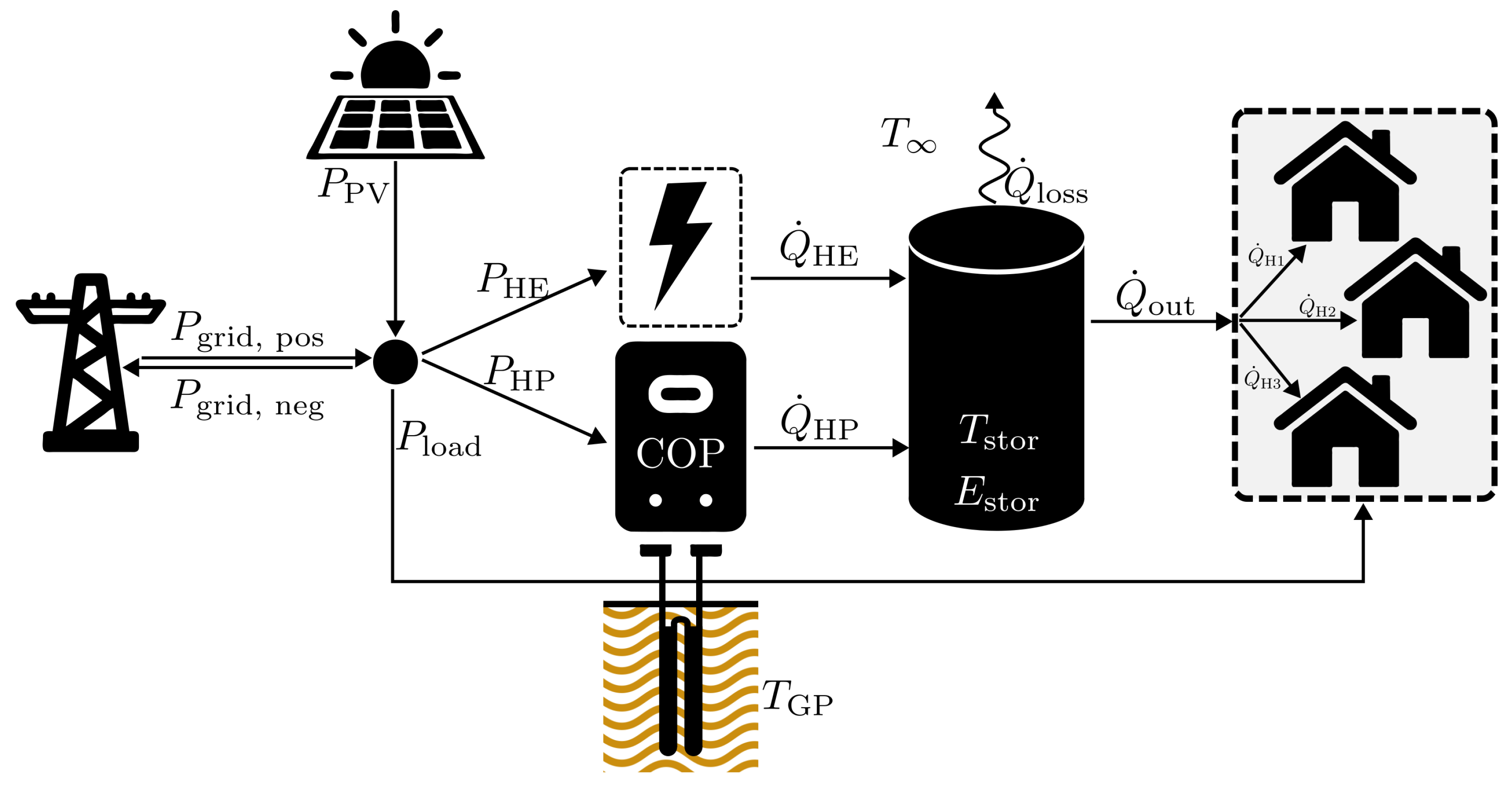
Figure 2.
Heating load (kW) of the EC throughout the investigated year, depicted with the applied train-test split.
Figure 2.
Heating load (kW) of the EC throughout the investigated year, depicted with the applied train-test split.
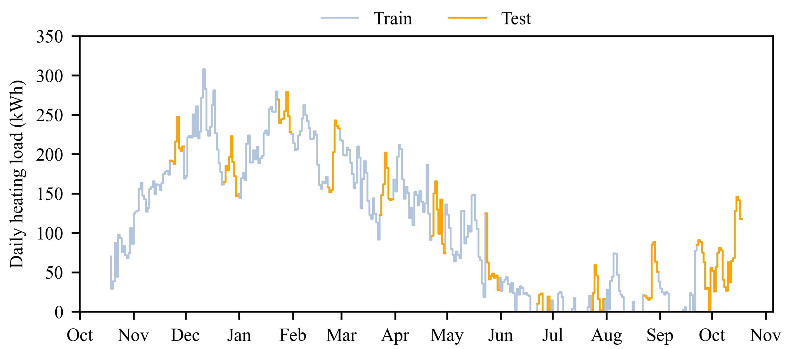
Figure 3.
Architecture of the DQN framework illustrating the interaction between the agent and the environment through states, actions, and rewards. The design incorporates a policy network and a target network for Q-value estimation, experience replay for sample efficiency, and soft target updates to enhance training stability.
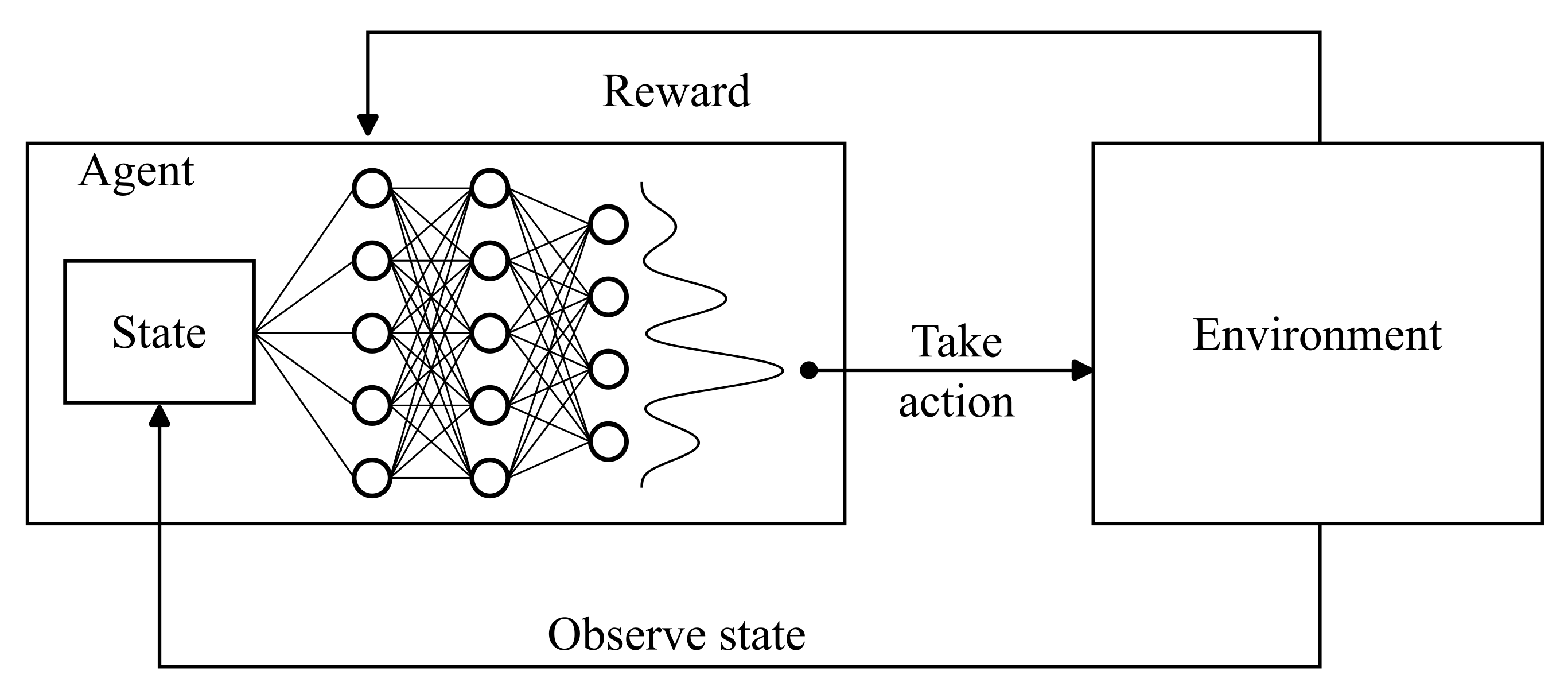
Figure 4.
Electrical energy flows inside the hub with the price signal. Panel a shows the RL model, and panel c shows the MILP model. Both panels depict the flows of electrical power from the photovoltaic system and the grid into the node, and the consumption by the load , heat pump , and heating element , as well as the feed-in to the grid . Panel b shows the varying electricity price signal and the constant feed-in tariff.
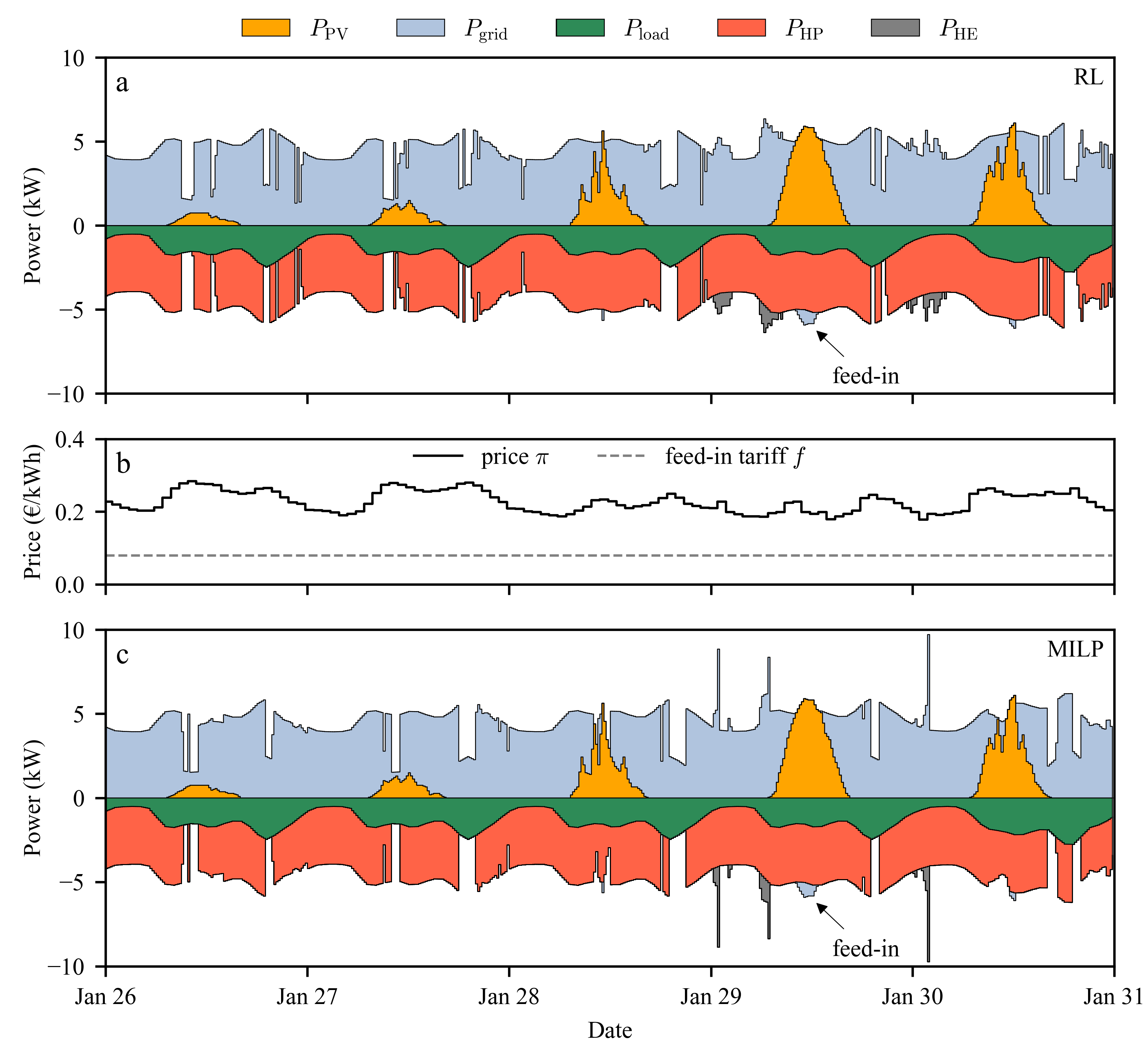
Figure 5.
Heat flows in and out of the TES, along with the internal temperatures. Panel a shows the RL model, and panel c shows the MILP model. Both panels depict heat input to the TES from the heat pump and the heating element , as well as heat output to the domestic heating load . Panel b shows the internal TES temperatures, including the upper and lower boundary temperatures and , in °C, along with the corresponding state of charge (SOC) in %.
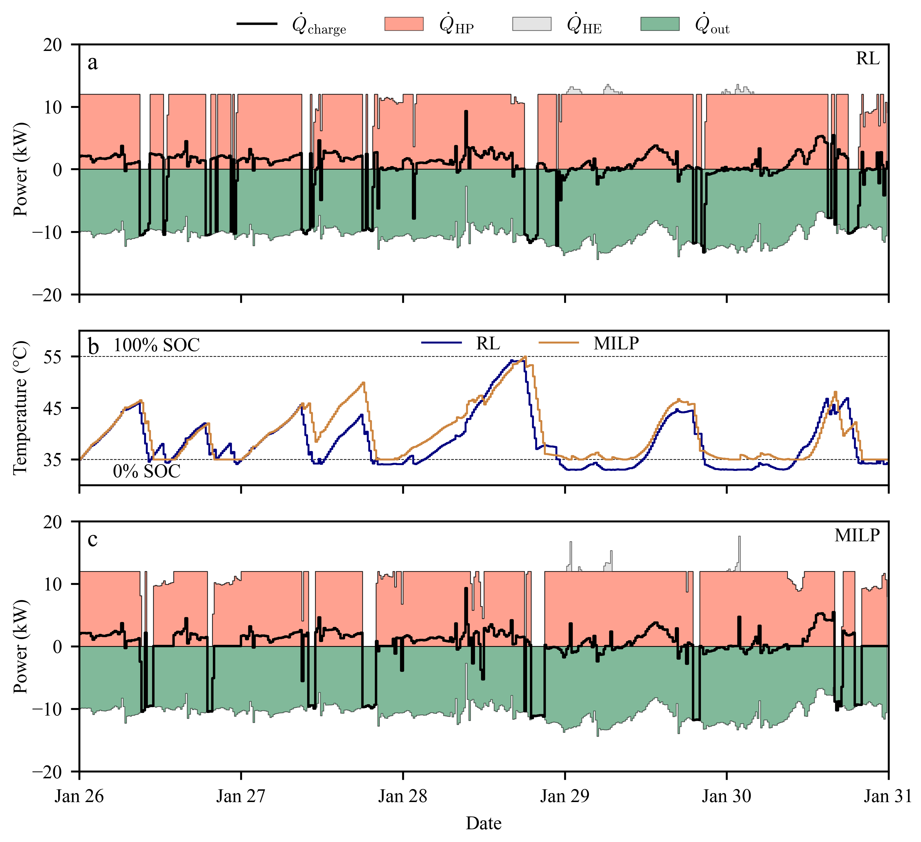
Figure 6.
KPIs in panel a, depicted as relative deviation from the reference scenario, and cumulative cost curves in panel b for the reference scenario, RL, and MILP. The KPIs include total costs in €, eq emissions in kg, grid energy usage in kWh, self-consumption ratio, and self-sufficiency ratio.
Figure 6.
KPIs in panel a, depicted as relative deviation from the reference scenario, and cumulative cost curves in panel b for the reference scenario, RL, and MILP. The KPIs include total costs in €, eq emissions in kg, grid energy usage in kWh, self-consumption ratio, and self-sufficiency ratio.
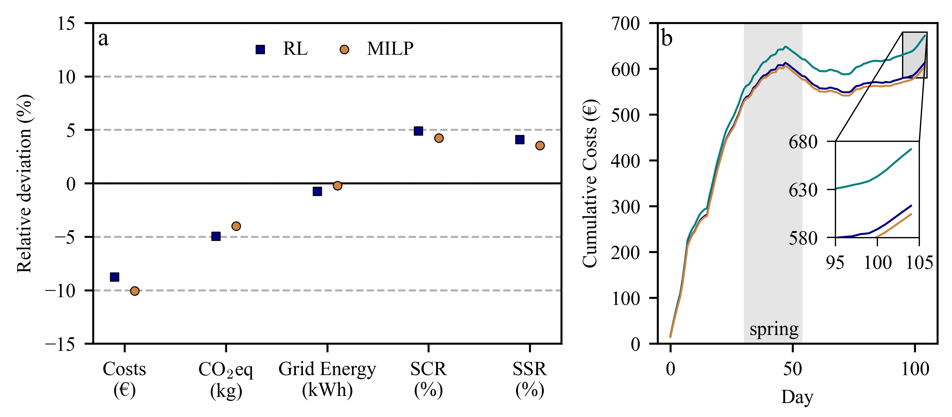
Table 1.
Overview of the data types used for simulation and optimization.
| Variable | Data Type | Source |
|---|---|---|
| Geothermal probe temperatures () | on-site | measured locally |
| Heat requirements () | on-site | measured locally |
| Electricity prices () | historical | EXAA market spot prices [26] |
| Feed-in tariffs (f) | historical | local feed in tariffs [27,28] |
| Carbon intensity | historical | Electricity Maps [29] |
| Electrical load (non-heating) () | synthetic | standard load profiles [30] |
| Photovoltaic power output () | synthetic | Geosphere Austria [31] |
| Seasonal classification | synthetic | binary encoding of seasons |
Table 2.
Seasonal encoding based on calendar months. Each season is represented by a binary feature.
Table 2.
Seasonal encoding based on calendar months. Each season is represented by a binary feature.
| Binary Indicator | Season | Active Months |
|---|---|---|
| Spring | March, April, May | |
| Summer | June, July, August | |
| Autumn | September, October, November | |
| Winter | December, January, February |
Table 3.
Model Parameters.
| Description | Parameter | Value | Unit |
|---|---|---|---|
| Resolution | 0.25 | h | |
| Storage capacity | 1.298 | kWh/K | |
| Storage lower temperature bound | 35 | ∘C | |
| Storage upper temperature bound | 55 | ∘C | |
| Ambient temperature | 20 | ∘C | |
| Min. heating power heat pump | 0 | kW | |
| Max. heating power heat pump | 12 | kW | |
| Max. heating power heating element | 6 | kW | |
| Proportional gain | 12 | – | |
| Equivalent emissions | CO2eq (Solar) | 0 | kg CO2eq/kWh |
| Heat transfer coefficient | h | 0.287 | K |
| TES surface area | A | 6 |
Table 4.
Comparison of absolute Key Performance Indicators.
| KPI | REF | RL | MILP |
|---|---|---|---|
| Costs (€) | 671.71 | 612.94 | 604.13 |
| eq (kg) | 929.88 | 883.91 | 892.58 |
| Grid Energy (kWh) | 1491.63 | 1480.32 | 1488.23 |
| SCR (%) | 28.76 | 33.66 | 33.01 |
| SSR (%) | 19.58 | 23.69 | 23.14 |
Disclaimer/Publisher’s Note: The statements, opinions and data contained in all publications are solely those of the individual author(s) and contributor(s) and not of MDPI and/or the editor(s). MDPI and/or the editor(s) disclaim responsibility for any injury to people or property resulting from any ideas, methods, instructions or products referred to in the content. |
© 2025 by the authors. Licensee MDPI, Basel, Switzerland. This article is an open access article distributed under the terms and conditions of the Creative Commons Attribution (CC BY) license (http://creativecommons.org/licenses/by/4.0/).
Copyright: This open access article is published under a Creative Commons CC BY 4.0 license, which permit the free download, distribution, and reuse, provided that the author and preprint are cited in any reuse.


