
Submitted:
21 November 2024
Posted:
21 November 2024
You are already at the latest version
Abstract
This paper presents a nonlinear velocity observer of the tether deployment using the Immersion and Invariance technique, and the velocity observer design problem is recast as a problem of designing an attractive and invariant manifold inside the Hamiltonian framework. The passivity-based control theory is used to define an expected Hamiltonian function, and the stability of the designed velocity observer is addressed by using the passivity-based methodology. Finally, a simple tension control law with measurable and unmeasurable states is employed for controlling the tether deployment, where the unmeasurable states use the proposed velocity observer. Numerical simulations demonstrate that the proposed velocity observer is working successfully. Sensitivity analyses are conducted to test the effectiveness and robustness of the proposed velocity observer.
Keywords:
tether deployment
; velocity observer
; immersion and invariance
; hamiltonian framework
; passivity-based control
1. Introduction
The space tether technology has been applied in a wide variety of applications, such as propulsion systems [1,2,3], power generation [4,5], micro-gravity experimentation [6,7], and tether transportation systems [8,9,10]. The issue of the deployment and retrieval of space tethers is crucial to space tether missions [11,12,13,14]. Many advanced control strategies have been applied to achieve a stable and fast deployment; however, it is difficult to achieve it entirely successful because the libration angle of the tether changes dramatically with a fast speed under the Coriolis force and other perturbed disturbances [15,16].
In past decades, many efforts have been devoted to designing the control law using different control methodologies, and they can be categorized into two parts in terms of measurable and unmeasurable states: full-state feedback [15,17,18,19] and partial-state feedback [16,20]. Among them, the tension control law with full-state feedback has been proven to be successful in realistic space missions [6,12,15]. For example, a mission function-based control law was proposed to suppress the libration motion in the tether deployment process [12]. Furthermore, a fractional-order term replacing the corresponding integer-older term inside Pradeep’s tension control law [21] was applied to ensure a stable and fast deployment dynamic [15], and it is theoretical proved that the fractional-order is a subset of the integer-order counterpart and has a more stable region. Recently, to ensure explicit non-negative velocity constraint of tether length, a novel tension control law based on the invariance principle of the control system is proposed [17], and numerical simulation results present that the tether deployment is smooth and faster and the velocity of tether length is kept positive. Furthermore, the sliding mode control method [19] was also adapted in the deployment and retrieval process to address robustness against external disturbance and low sensitivity of model parameter uncertainties. Following that, a combination of fractional-order and sliding model controllers was also proposed to address the unmodeled dynamics of the tether deployment [18,22]. For example, the frictional force between the loading equipment and the tether. However, it is noted that there is one assumption in the previous controller, the feedback state is directly measurable, which has some challenging in a real mission due to the lack of available sensors [6]. In addition to the full-state feedback control law, a tension control law with partial-state feedback is highly desirable, as mentioned in Refs. [20,23]. For example, a simple analytical control law with partial state feedback based on the energy storage function is proposed in Ref. [16]. Among it, only the tether length and its rate are measurable. Numerical simulation results demonstrate that a better performance is achieved against the fractional-order counterpart [15].
In addition to the controller design using different methodologies, there are also some works related to the measurement model of the measurable state. As presented in Refs. [13,24], the states of tether deployment dynamics were estimated based on the measurement data from onboard cameras and GPS. It is noted that the estimated state may be inaccurate, leading to accidentally unsuccessful tether deployment. For example, the YES2 experiment was not entirely successful because of errors in estimating the tether velocity [25]. It is important that the estimation algorithm of the unmeasurable state be adopted to ensure successful tether deployment. Many efforts have been devoted to developing the estimation algorithm for the unmeasurable state of the tether system. For example, the Kalman filter algorithm was employed to estimate the unmeasurable states of the tether system [23,26,27]. It is simple, straightforward, and easy to implement. However, the defect of this algorithm is apparent, and a significant computational load is required to process a set of sampling points [26]. The Immersion and invariance (I&I) technique [28] has also been explored to estimate the unmeasurable states of the STS [29] because it is a constructive methodology that has been widely adopted in many dynamic nonlinear systems [30]. The measurement model of the unmeasurable state can be analytically derived by solving a nonlinear partial differential equation, and it is proved to be estimated accurately [31]. For example, a velocity observer using I& I technique is proposed to estimate the libration angle (in-plane and out-of-plane) velocities of an electrodynamic tether system.
In this paper, the I&I technique is applied to design the velocity observer for the tether deployment. However, compared to the work presented in [29], it is difficult and challenging to construct a Lyapunov candidate because it highly depends on the author’s experience and familiarity with the target system. In order to address the complexity of constructing a Lyapunov candidate, the velocity observer error system is converted into a generalized Hamiltonian framework. To the best of the authors’ knowledge, this is the first attempt to present a velocity observer design inside a Hamiltonian framework. Inspired by the Hamiltonian theory and passivity method [20], an attractive and invariant manifold observer is converted into an extended Hamiltonian framework. Therefore, the velocity observer design problem is recast as the problem of designing an attractive and invariant manifold inside a Hamiltonian framework, and the attractivity of the proposed manifold can be achieved by solving a formed partial differential equation [32]. The passivity-based control can be directly used to derive an expected Hamiltonian function, and the Hamiltonian storage energy function can be taken as an ideal Lyapunov candidate [33].
The rest of the paper is organized as follows: Section 2 illustrates the dynamics of tether deployment. Section 3 proposes a nonlinear velocity observer and presents the stability proof, and the proving process was explained in two parts to enhance readability. In Section 4, numerical simulations are carried out to show the effectiveness and robustness of the proposed velocity observer. Finally, Section 5 concludes the paper.
2. Dynamic System Description and Preliminaries
In this paper, as shown in Figure 1, the space tether system is supposed to be a long and thin cable with two connecting spacecraft at each end. As presented in Refs. [15,22], the system is modeled as a dumbbell model consisting of two end spacecraft connected by a straight tether with a variable length , and the spacecrafts are modelled as lumped masses without attitude dynamics. We focus on the in-plane motion since the out-of-plane motion is small compared with its counterpart [20]. The mass of the tether can be ignored compared with the mass of the spacecraft. The Lagrange’s equation is applied to derive the governing equations of the tether deployment [12,16], and they are written as,
where symbol represents derivative with respect to time, indicates instantaneous tether length, is the in-plane (pitch) angle, denotes orbital rate of the system, is the tension of tether. is the equivalent mass with and being the masses of the main and sub spacecraft, respectively.
The following non-dimensional variables are defined to non-dimensionalize the Equation (1),
where denotes the dimensionless tether length with being the total length of the tether, and it satisfies . represents the dimensionless time and is the angular velocity of the system.
Substituting Equation (2) into (1) generating the following dimensionless equations,
where symbol denotes the derivative with respect to the dimensionless time .
Here, rewrite Equation (3) into a compact form,
with
where and are vectors of position and its rate, respectively, and is control input vector. is generalized inertia matrix, is Coriolis and Centrifugal forces matrix. force vector due to its gravity.
The following variables are defined to implement coordinate transform,
where is a introduced factorization of the generalized inertia matrix [34], namely
The following mappings and can be defined,
It is noted that the following values and listed in Equation (8) are known values that means the above defined mappings are known.
Taking derivative with respect to non-dimensional time for Equation (6), then the following variables with a state-space form are formed,
where is a mapping matrix, and it consists of two parts: the constant part and the parameter part.
The following lemma are given firstly before presenting the velocity observer, the interested readers can found detailed proofing part in [34].
Lemma 1.The mapping matrixis defined as,
where decomposes into two parts, the constant part and the parameter part ,
where is a constant and skew-symmetric matrix. have the following three properties,
- (i)
- is a skew-symmetric matrix .
- (ii)
- is a linear function about the first argument for and .
- (iii)
- There exists mapping , for all .
3. Proposed Velocity Observer
In this section, a detailed derivation process of the proposed velocity observer is presented.
Theorem.Consider the Equation (4), a exponentially convergent velocity observer will be presented, with unmeasurable state, measurable output stateand input,
where is designed observer and denotes an existing smooth observer mapping.
3.1. Velocity Observer Design
In this paper, the immersion and invariance (I&I) theory is employed to design the velocity observer [32,35]. Here, a manifold for the tether system listed in Eq.(9) is given,
where denotes the dynamic part of the observer state, is a defined mapping will be given later and is an estimate of the state ,
Then, to ensure the proposed manifold is attractive and invariant, the off-the-manifold coordinate is given,
where when approaches to zero.
Combining Equation (9) and taking derivatives with respect to the time of Equation (15),
Based on the Equation (16), let the dynamics of as,
where , and are Jacobian matrices of the mapping with respect to , and , respectively. is called dynamic scaling factor, and it will be given in later sections. and are estimated error with respect to the state x and y, respectively.
Substituting the Equation (17) into Equation (16) generating the following equation,
The following dynamic equations of the observer are defined as,
where and are positive gains, and they will be given in numerical simulation section.
Taking derivatives of Equation (18) generating the following equations,
3.2. Dynamic Scaling Factor for Domination
A dynamic scaling factor is introduced to transform the off-the manifold listed in Equation (19), Equation (19) is rewritten as,
Also, Equation (21) is rewritten in terms of dynamic as dynamic scaling factor as,
Then, a Hamiltonian form by combining Equations (22) and (23) as written as,
where is a new state vector of the observer dynamics. is a Hamiltonian storage energy function listed in Eq.. and are the interconnection and damping matrices, respectively. It is noted that interconnection matrix is a skew-symmetric matrix , and is a damping matrix that needs to be positive definite, which means the energy is extracted out of the system.
As noted in Equations (26) and (27), the is unknown and needed to be solved. In this paper, an ideal is given based on the approximation solution [36],
where is a positive gain to be selected, and is a full rank inverse of the .
As listed in Equation (27), the first element entry inside the damping matrix is rewritten as,
where is an identity matrix with a size .
Here, an error damping is defined as,
Then, the error mapping can be factorized as,
where and can be explained as the role of disturbance compensation mapping for the observer states.
where and can be calculated as follows.
where , and . Thereby, we can obtain the following equations,
Then, based on Equations (30)–(33), Equation (29) and Equation (29) can be rewritten as,
Remark 2: As listed in Equation (28) is given, the approximate solution of a partial differential equation is given. Furthermore, as listed in Equation (36), the damping matrixhas been converted specially. Noting that the Hamiltonian structure is maintained, which satisfies the property of the Hamiltonian theory. Therefore, the transformed Hamiltonian function (36) will be used to prove the stability of the proposed observer.
3.3. Domination by High-Gain Injection and Stability
In this section, the introduced scaling factor is explicitly given, and the Lyapunov stability analysis of the designed velocity observer is carried out.
Taking time derivative of the Hamiltonian function generating the following equation,
where and are defined as positive gain matrices. It is easily noted that we can obtain if the property of is given.
Then, the scaling factor r is defined as,
with , and notice that the factor satisfied [31], and , which can achieve the exponential convergence of the observer system.
Defining a positive-definite function , and its derivative with non-dimensional time is written as
where denotes the matrix induced 2-norm, and the Young’s inequality is used to get the second bound.
Substituting Equation (39) into Equation (40) leading to the following equation,
where . It is noticed that the coordinate z converges to zero exponentially.
To ensure the boundedness of the scaling function r listed in Equation (22), the additional positive function is defined as follows,
Then, a proper Lyapunov candidate function for the extended system is written as,
Taking the derivative leading to the following equation,
As listed in Equation (34), the error mappings and approaches zero. And two mappings are defined as and .
Here, to ensure the boundness of factor r, the gains and are chosen as,
where are positive constants.
Substituting Equation (45) into Equation (44) leading to the following equations,
where being the minimal value between the gains , , and .
Based on Equation (46), the observer system is exponentially stable. Meanwhile, it is evident that scaling function r has a finite boundedness, and it can be used for the robustness of the observer system against disturbed mapping . Therefore, the state error will exponentially converge to zero, and the component is the estimate of state .
Remark 3:It is worth noting that the proposed observer system is converted into a Hamiltonian framework; the method for setting the gain functionsandis different from the method presented in [34], which needs to construct an intermediate term. In this paper, the detailed process is not presented here. Meanwhile, the stabilization via the I&I method is combined with passivity-based theory in this work, with a suitable Hamiltonian storage function.
Remark 4: It should be pointed out that the defined constant gainsare needed to be explicitly and carefully chosen. Different gain parameters will affect the performance of the proposed observer significantly, which will be investigated inside the numerical simulation section. Furthermore, sensitivity analysis is recommended for the proposed velocity observer with different mission requirements.
4. Numerical Cases
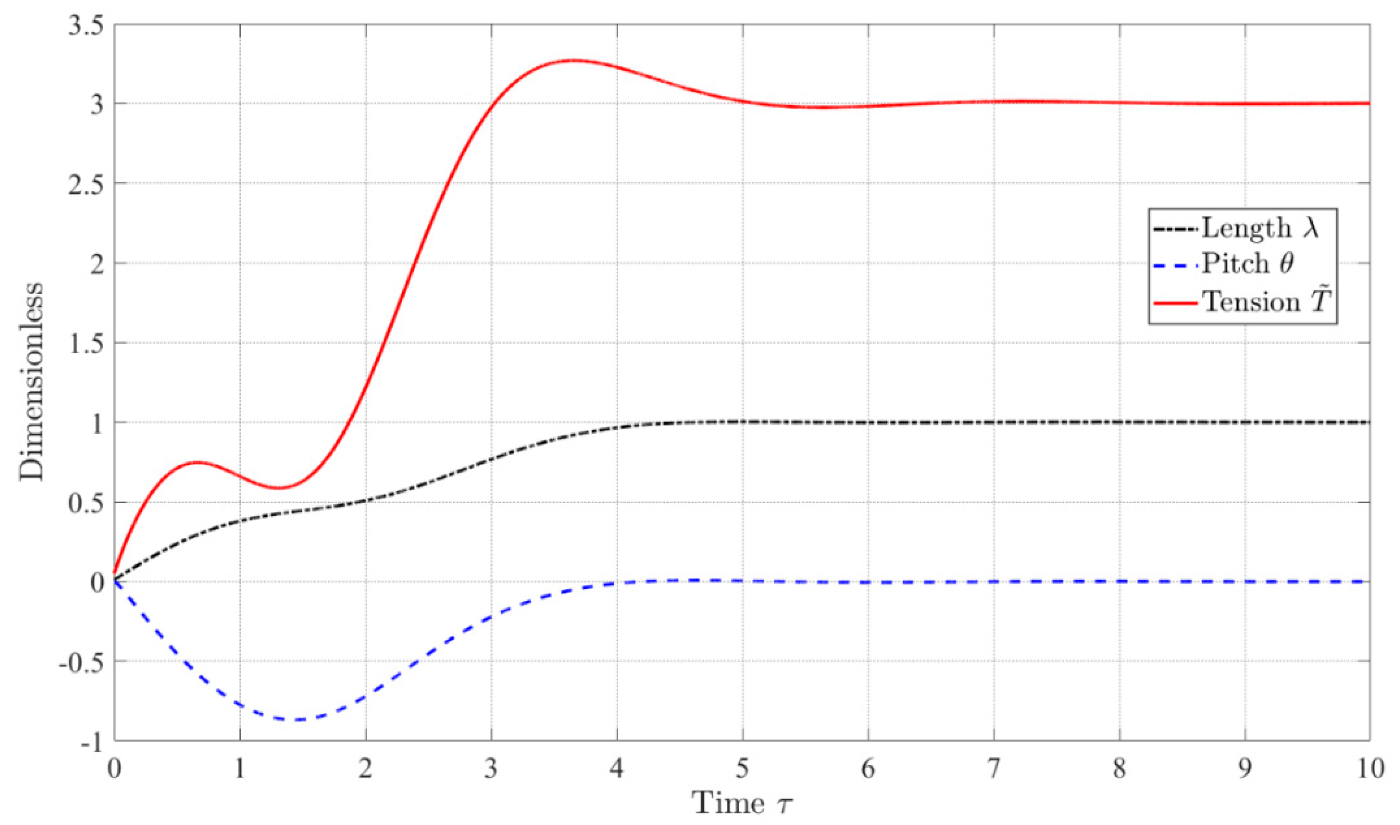
In this section, the proposed velocity observer is evaluated via the numerical simulation. Here, the tension controller proposed in Ref. [37] is used to control the tether deployment. Note that the tension controller is only used as the control input for the proposed velocity observer. In this paper, the STS is in a circular orbit with altitude 220 km, and the initial conditions of the tether deployment are set as, , , and , and the desired state are set as, , . For simplicity, the positive gains of the proposed controller are set the same as the values presented in Ref. [37]. Figure 1 shows time histories of the non-dimensional tether length and in-plane libration under the implemented controller when these two velocity terms and are temple supposed to be known. As proposed in Section 3, the velocity terms and inside the tension controller will be replaced by the proposed observed velocity and listed in Equation (24).
Figure 2.
Time histories of non-dimensional tether length, in-plane libration angle and input tension.
Figure 2.
Time histories of non-dimensional tether length, in-plane libration angle and input tension.
4.1. Case 1: Observer with Different Gains
In this section, as listed in Equation (36), the velocity gain affecting the performance of the proposed velocity observer is investigated. As listed in Table 1, six different values of gain are considered. The simulation parameters, the gains of the observer, and the initial conditions of the STS are given in Table 1. It should be mentioned that the relationship between the observer state and can be found in Equation (6). The simulation results are shown in Figure 3, Figure 4, Figure 5, Figure 6, Figure 7 and Figure 8, and the results are illustrated by the state and the velocity state of the STS.
Figure 3 and Figure 4 show time histories of the estimated position and velocities and with different gains . It is easily found that the proposed velocity observer estimates the velocity successfully. However, it is found that the dynamic behavior of the tether length rate and libration rate caused by different gain values are obviously different. For example, as shown in Figure 5, a bigger gain makes the estimated velocity of the tether length converge to the actual value faster. However, its impact on the estimated velocity of the libration angle is inverse. Furthermore, as shown in Figure 5b, the estimated angle velocity has some overshoot with both small and big gain values, such as and . The system response is slower and prone to overshooting when the gain is too small. Conversely, when the gain is too large, the system will be too sensitive, and overshoot will also be intensified. Therefore, the dynamic behavior phenomenon suggests optimizing the gain value to balance its effect on the estimated velocities. Figure 6 depicts the time histories of the errors of velocities and . It is easily found that the errors of velocity exponentially approach zero. In addition, Figure 7 shows time histories of the dynamic scaling factor under different values of the gain . It shows that the scaling factor has a boundedness of , and it also suggests a bigger gain value making the scale r converge faster.
4.2. Observer with Input Measurement Noise
In this section, the measurement noise is considered for the measurable state to demonstrate the robustness of the proposed velocity observer. As listed in Equation (47), disturbance noises and are added to the measurement of the input state and . The simulation parameters and the initial conditions are the same values in Table 1. Figure 8 shows the time histories of the measurement state and under the proposed noise model.
Figure 9 and Figure 10 show time histories of the estimated velocity of the tether length and the velocity of the libration angle under the applied disturbance. Also, the dynamic behaviour of the proposed estimated velocities and with different gain value are investigated. A noticeable chatting phenomenon is easily found when a big value of gain is chosen. Furthermore, it oscillates around the reference velocity and is not converged. Therefore, a big gain is not expected when the measurement noise model is considered. The same dynamic behavior of the pith angle velocity (overshoot) is also found when a small gain is applied. Figure 11 shows the rapid convergence of the estimated velocities and to the referred velocities when the velocity gain is set as 1.0, which demonstrates the robustness of the proposed observer against measurement noise. The shapes of the estimated velocity value are smooth, as expected, even when the measurement noise is considered. Therefore, the velocity gain will be chosen in the following simulations to illustrate the performance behavior.
4.3. Observer Under the Different Initial Conditions
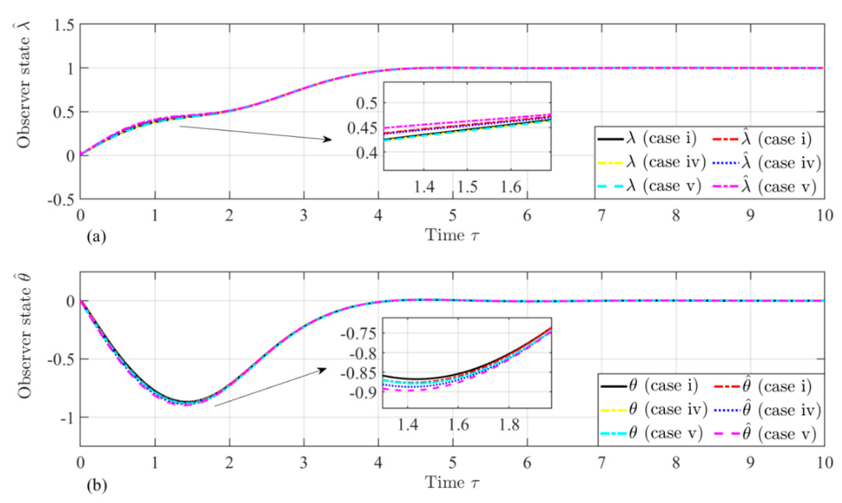
In the previous section, as listed in Table 1, the initial conditions are known values. In this section, different sets of initial conditions of the estimated velocities and impacting the performance of the proposed velocity are investigated. Here, the velocity gain is set as 1.0, and the initial value of the scale factor is set as 1.5. The other initial conditions are set the same as the values listed in Table 1. Table 2 lists different sets of the initial conditions used in this section, and six numerical simulations are carried out. In the first three cases (i, ii, and iii), the in-plane libration rate is supposed to be zero to avoid the tether winding up in deployment process [17]. Figure 12 shows the time histories of the proposed observer state and , and an expected discrepancy at initial stage between the estimated and actual states is observed due to the difference between the estimated and referred velocities. Figure 13 shows that the time histories of the proposed velocity state and , and it shows the estimated velocities converge to the reference velocities in fast. It can be concluded that the effect of the initial estimated velocity of the deployment on the proposed observer is trivial.
To further validate the performance of the proposed velocity observer, the velocity of the tether libration angle is not zero, which may happen in a real mission. As listed in Table 2, another three numerical simulations are carried out. The same dynamic behavior between the observed state and the referred state is observed due to the initial difference between the estimated and referred velocities. Figure 15 shows that the estimated velocities also converge with the reference velocities, and their behavior is the same as that of the initial libration rate, which is zero. Finally, we can conclude that the proposed velocity observed is working well and can be applied for estimating the unmeasurable velocity term and inside the tension controller in a realistic mission analysis.
Figure 14.
Time histories of the state and of the observer dynamics with angle rate at different initial velocities.
Figure 14.
Time histories of the state and of the observer dynamics with angle rate at different initial velocities.
5. Conclusions
This paper proposes a nonlinear velocity observer of tether deployment based on the Immersion and Invariance technique. The velocity observer system is transformed into an extended Hamiltonian formulation by introducing the error of the state and scaling dynamic factor. The stability of the proposed velocity observer is proved using the passivity-control methodology under the Hamiltonian framework. Furthermore, a crucial partial differential equation and a simple gain function are invoked in the designing process. Finally, the proposed velocity observer is applied to simulate the tether deployment. Numerical simulations are carried out to demonstrate the effectiveness and robustness of the proposed velocity observer. Sensitivity analyses considering measurement disturbance are carried out to characterize the robustness of the proposed velocity observer.
Funding
This study was financially supported by the National Natural Science Foundation of China (Grant No. 12202228).
References
- Borderes-Motta, G.; de Haro-Pizarroso, G.; Li, G.; Yu, H.; Zhu, Z.H.; Sarego, G.; Colombatti, G.; Lorenzini, E.C.; McTernan, J.K.; Gilchrist, B.E.; et al. Cross-verification and benchmarking analysis of electrodynamic tether simulators. Acta Astronautica 2023, 208, 381–388. [Google Scholar] [CrossRef]
- Li, G.; Zhu, Z.H.; Du, C. Stability and control of radial deployment of electric solar wind sail. Nonlinear Dynamics 2021, 103, 481–501. [Google Scholar] [CrossRef]
- Du, C.; Zhu, Z.H.; Li, G. Analysis of thrust-induced sail plane coning and attitude motion of electric sail. Acta Astronautica 2021, 178, 129–142. [Google Scholar] [CrossRef]
- Sidhu, L.; Zhu, G. Space Debris Mitigation: Integration of Carbon Nanotube Cold Cathode Electron Emission with Electrodynamic Tether Payload for Rapid Deorbiting of Nanosatellites. In 2024 Regional Student Conferences.
- Liu, J.; Li, G.; Zhu, Z.H.; Liu, M.; Zhan, X. Automatic orbital maneuver for mega-constellations maintenance with electrodynamic tethers. Aerospace Science and Technology 2020, 105, 105910. [Google Scholar] [CrossRef]
- Misra, A.K. Dynamics and control of tethered satellite systems. Acta Astronautica 2008, 63, 1169–1177. [Google Scholar] [CrossRef]
- Lorenzini, E.C. A three-mass tethered system for micro-g/variable-g applications. Journal of Guidance, Control, and Dynamics 1987, 10, 242–249. [Google Scholar] [CrossRef]
- Li, G.; Zhu, Z.H.; Shi, G. A novel looped space tether transportation system with multiple climbers for high efficiency. Acta Astronautica 2021, 179, 253–265. [Google Scholar] [CrossRef]
- Yang, J.; Wang, Q.; Zhang, Z.; Liu, Z.; Xu, S.; Li, G. Dynamic modeling and analysis of the looped space tether transportation system based on ANCF. International Journal of Mechanical System Dynamics 2022, 2, 204–213. [Google Scholar] [CrossRef]
- Huang, J.; Misra, A.K. Controlled deployment of a long tether to operate as a partial space elevator. Astrodynamics 2024, 8, 311–321. [Google Scholar] [CrossRef]
- Bindra, U.; Zhu, Z.H. Development of an Air-Bearing Inclinable Turntable for Testing Tether Deployment. In AIAA Guidance, Navigation, and Control Conference.
- Fujii, H.; Ishijima, S. Mission function control for deployment and retrieval of a subsatellite. Journal of Guidance, Control, and Dynamics 1989, 12, 243–247. [Google Scholar] [CrossRef]
- Yamagiwa, Y.; Fujii, T.; Nakashima, K.; Oshimori, H.; Okino, T.; Komua, S.; Arita, S.; Nohmi, M.; Ishikawa, Y. Space experimental results of STARS-C CubeSat to verify tether deployment in orbit. Acta Astronautica 2020, 177, 759–770. [Google Scholar] [CrossRef]
- Fulton, J.; Schaub, H. Fixed-axis electric sail deployment dynamics analysis using hub-mounted momentum control. Acta Astronautica 2018, 144, 160–170. [Google Scholar] [CrossRef]
- Sun, G.; Zhu, Z.H. Fractional-Order Tension Control Law for Deployment of Space Tether System. Journal of Guidance, Control, and Dynamics 2014, 37, 2057–2062. [Google Scholar] [CrossRef]
- Wen, H.; Zhu, Z.H.; Jin, D.; Hu, H. Space Tether Deployment Control with Explicit Tension Constraint and Saturation Function. Journal of Guidance, Control, and Dynamics 2016, 39, 916–921. [Google Scholar] [CrossRef]
- Murugathasan, L.; Zhu, Z.H. Deployment control of tethered space systems with explicit velocity constraint and invariance principle. Acta Astronautica 2019, 157, 390–396. [Google Scholar] [CrossRef]
- Ma, Z.; Zhu, Z.H.; Sun, G. Fractional-order sliding mode control for deployment of tethered spacecraft system. Proceedings of the Institution of Mechanical Engineers, Part G: Journal of Aerospace Engineering 2019, 233, 4721–4734. [Google Scholar] [CrossRef]
- Ma, Z.; Sun, G.; Cheng, Z.; Li, Z. Pure-tension non-linear sliding mode control for deployment of tethered satellite system. Proceedings of the Institution of Mechanical Engineers, Part G: Journal of Aerospace Engineering 2018, 232, 2541–2551. [Google Scholar] [CrossRef]
- Kang, J.; Zhu, Z.H. A unified energy-based control framework for tethered spacecraft deployment. Nonlinear Dynamics 2019, 95, 1117–1131. [Google Scholar] [CrossRef]
- Pradeep, S. A new tension control law for deployment of tethered satellites. Mechanics Research Communications 1997, 24, 247–254. [Google Scholar] [CrossRef]
- Kang, J.; Zhu, Z.H.; Wang, W.; Li, A.; Wang, C. Fractional order sliding mode control for tethered satellite deployment with disturbances. Advances in Space Research 2017, 59, 263–273. [Google Scholar] [CrossRef]
- Tortora, P.; Somenzi, L.; Iess, L.; Licata, R. Small Mission Design for Testing In-Orbit an Electrodynamic Tether Deorbiting System. Journal of Spacecraft and Rockets 2006, 43, 883–892. [Google Scholar] [CrossRef]
- Wen, H.; Zhu, Z.H.; Jin, D.; Hu, H. Constrained tension control of a tethered space-tug system with only length measurement. Acta Astronautica 2016, 119, 110–117. [Google Scholar] [CrossRef]
- Aslanov, V.S.; Ledkov, A.S. 1 - Space tether systems: review of the problem. In Dynamics of Tethered Satellite Systems, Aslanov, V.S., Ledkov, A.S., Eds.; Woodhead Publishing: 2012; pp. 3–104.
- Li, G.; Zhu, Z.H. Estimation of flexible space tether state based on end measurement by finite element Kalman filter state estimator. Advances in Space Research 2021, 67, 3282–3293. [Google Scholar] [CrossRef]
- Li, G.; Zhu, Z.H. Model predictive control for electrodynamic tether geometric profile in orbital maneuvering with finite element state estimator. Nonlinear Dynamics 2021, 106, 473–489. [Google Scholar] [CrossRef]
- Astolfi, A.; Karagiannis, D.; Ortega, R. Nonlinear and adaptive control with applications; Springer: 2008; Volume 187.
- Wen, H.; Zhu, Z.H.; Jin, D.; Hu, H. Exponentially Convergent Velocity Observer for an Electrodynamic Tether in an Elliptical Orbit. Journal of Guidance, Control, and Dynamics 2016, 39, 1113–1118. [Google Scholar] [CrossRef]
- Xia, D.; Yue, X.; Wen, H. Output feedback tracking control for rigid body attitude via immersion and invariance angular velocity observers. International Journal of Adaptive Control and Signal Processing 2020, 34, 1812–1830. [Google Scholar] [CrossRef]
- Stamnes, Ø.N.; Aamo, O.M.; Kaasa, G.-O. A constructive speed observer design for general Euler–Lagrange systems. Automatica 2011, 47, 2233–2238. [Google Scholar] [CrossRef]
- Karagiannis, D.; Astolfi, A. Observer design for a class of nonlinear systems using dynamic scaling with application to adaptive control. In Proceedings of the 2008 47th IEEE Conference on Decision and Control, 2008, 9-11 Dec. 2008; pp. 2314–2319. [Google Scholar]
- Ortega, R.; van der Schaft, A.; Maschke, B.; Escobar, G. Interconnection and damping assignment passivity-based control of port-controlled Hamiltonian systems. Automatica 2002, 38, 585–596. [Google Scholar] [CrossRef]
- Astolfi, A.; Ortega, R.; Venkatraman, A. A Globally Exponentially Convergent Immersion and Invariance Speed Observer for N Degrees of Freedom Mechanical Systems. Proceedings of the 48h IEEE Conference on Decision and Control (CDC) held jointly with 2009 28th Chinese Control Conference 2009, 6508-6513.
- Karagiannis, D.; Sassano, M.; Astolfi, A. Dynamic scaling and observer design with application to adaptive control. Automatica 2009, 45, 2883–2889. [Google Scholar] [CrossRef]
- Romero, J.G.; Ortega, R. A Globally Exponentially Stable Tracking Controller for Mechanical Systems with Friction Using Position Feedback. IFAC Proceedings Volumes 2013, 46, 371–376. [Google Scholar] [CrossRef]
- Vadali, S.R. Feedback tether deployment and retrieval. Journal of Guidance, Control, and Dynamics 1991, 14, 469–470. [Google Scholar] [CrossRef]
Figure 1.
Schematic diagram of the space tether system.
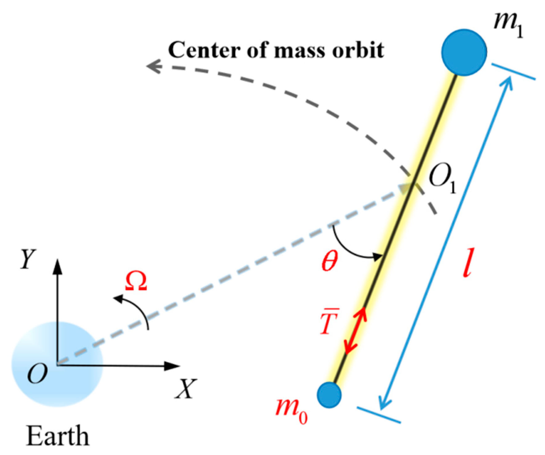
Figure 3.
Time histories of the state and of the observer dynamics.
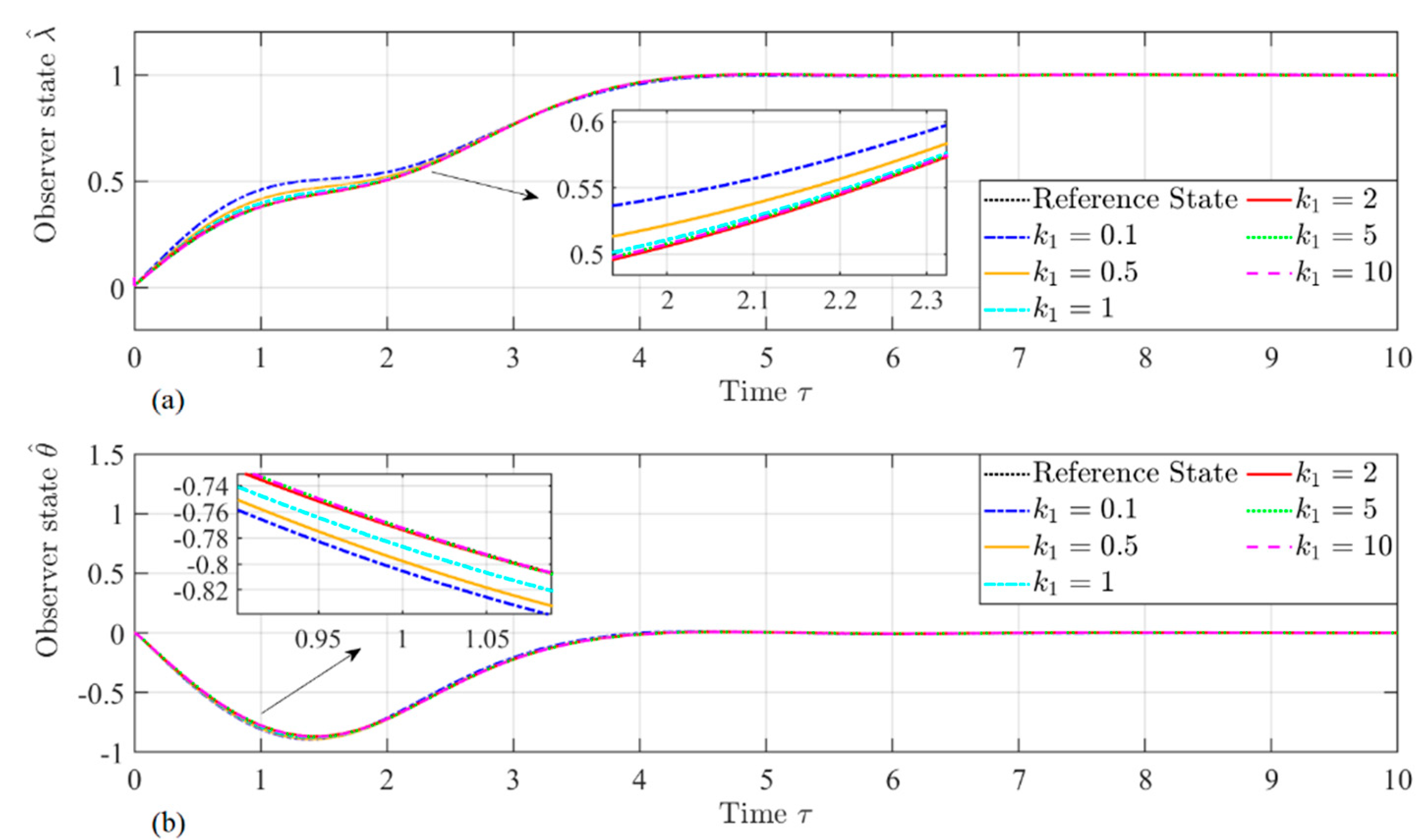
Figure 4.
Time histories of the estimated velocities and .
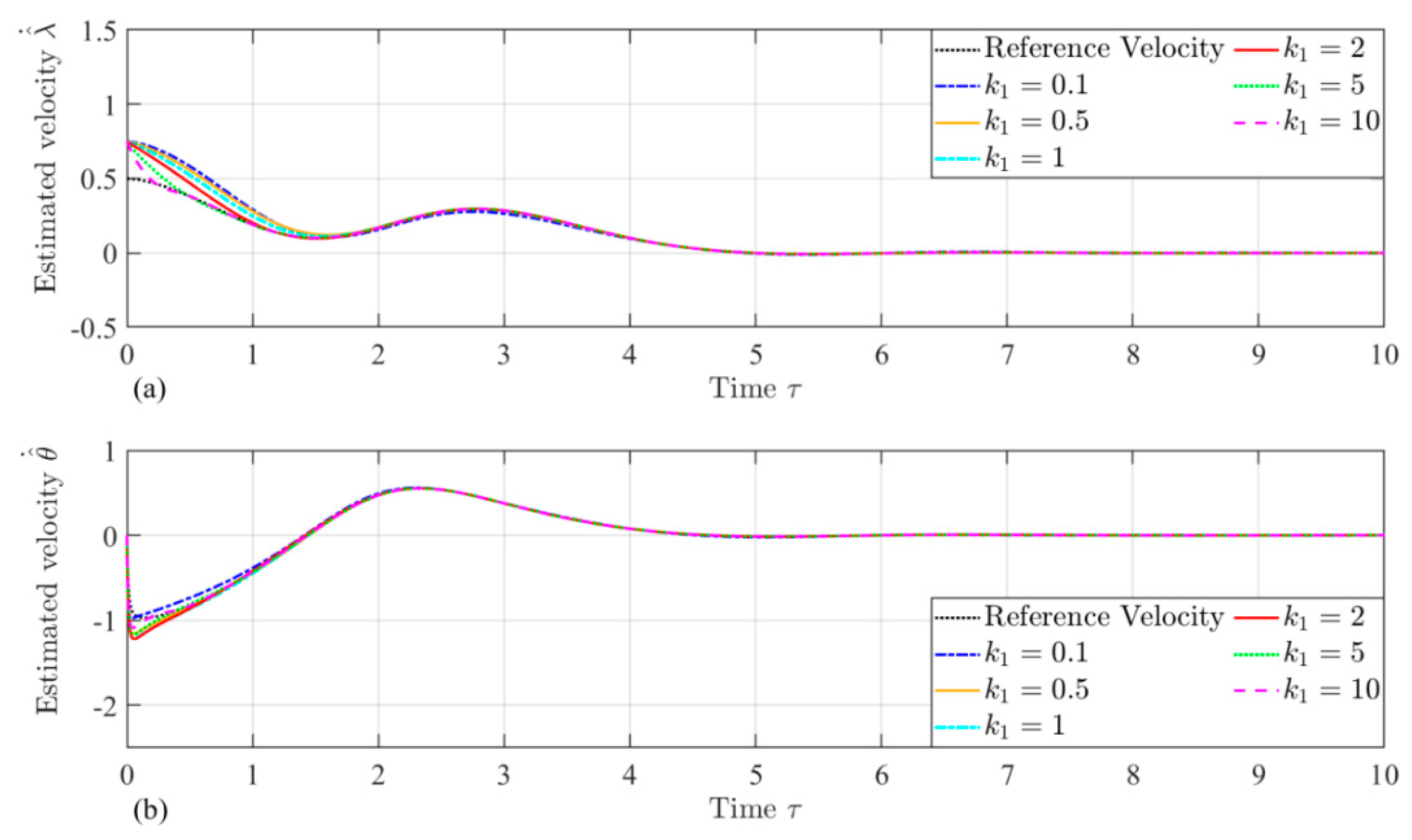
Figure 5.
Time histories of the estimated velocities and (Magnified).
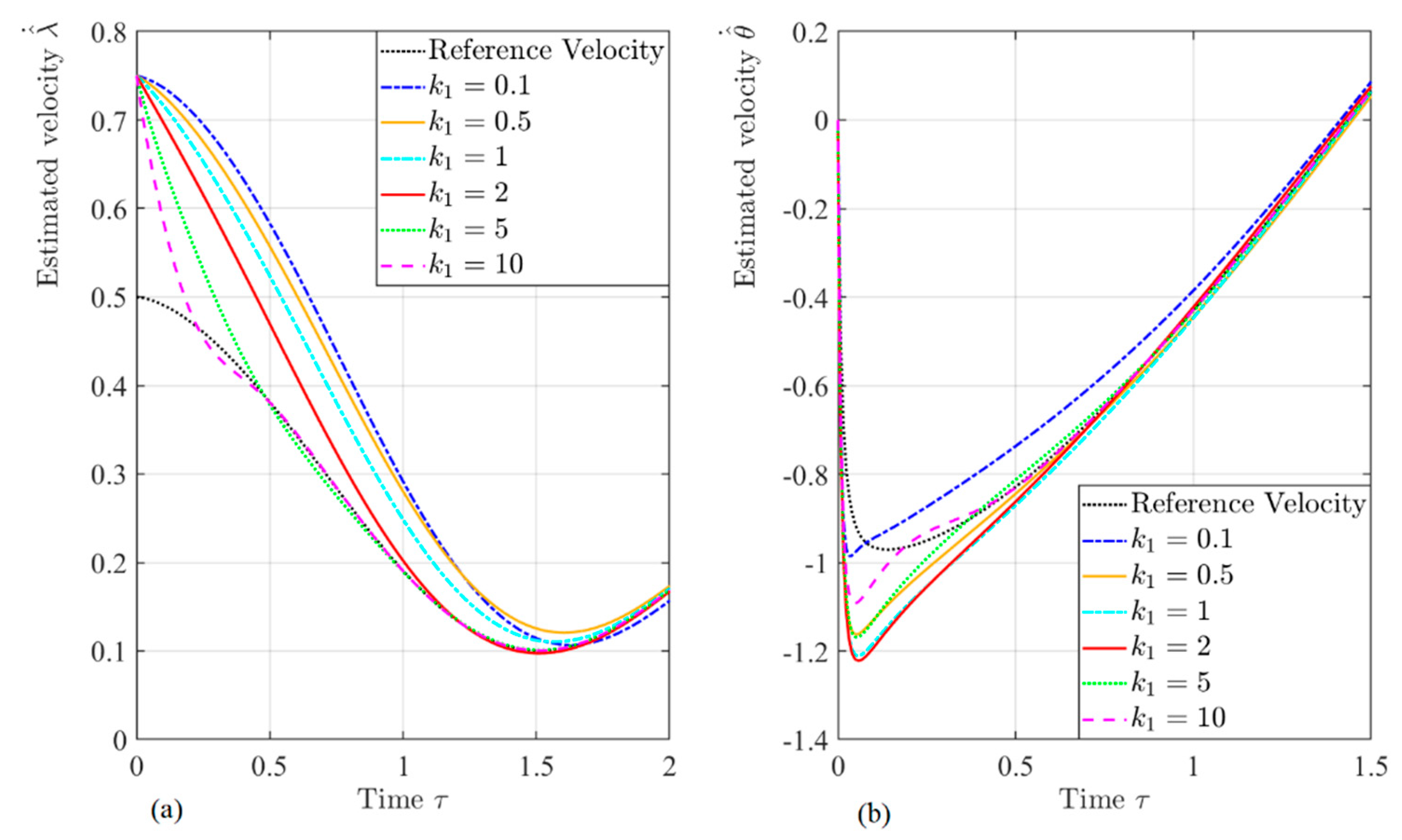
Figure 6.
Time histories of error of the estimated velocities and .
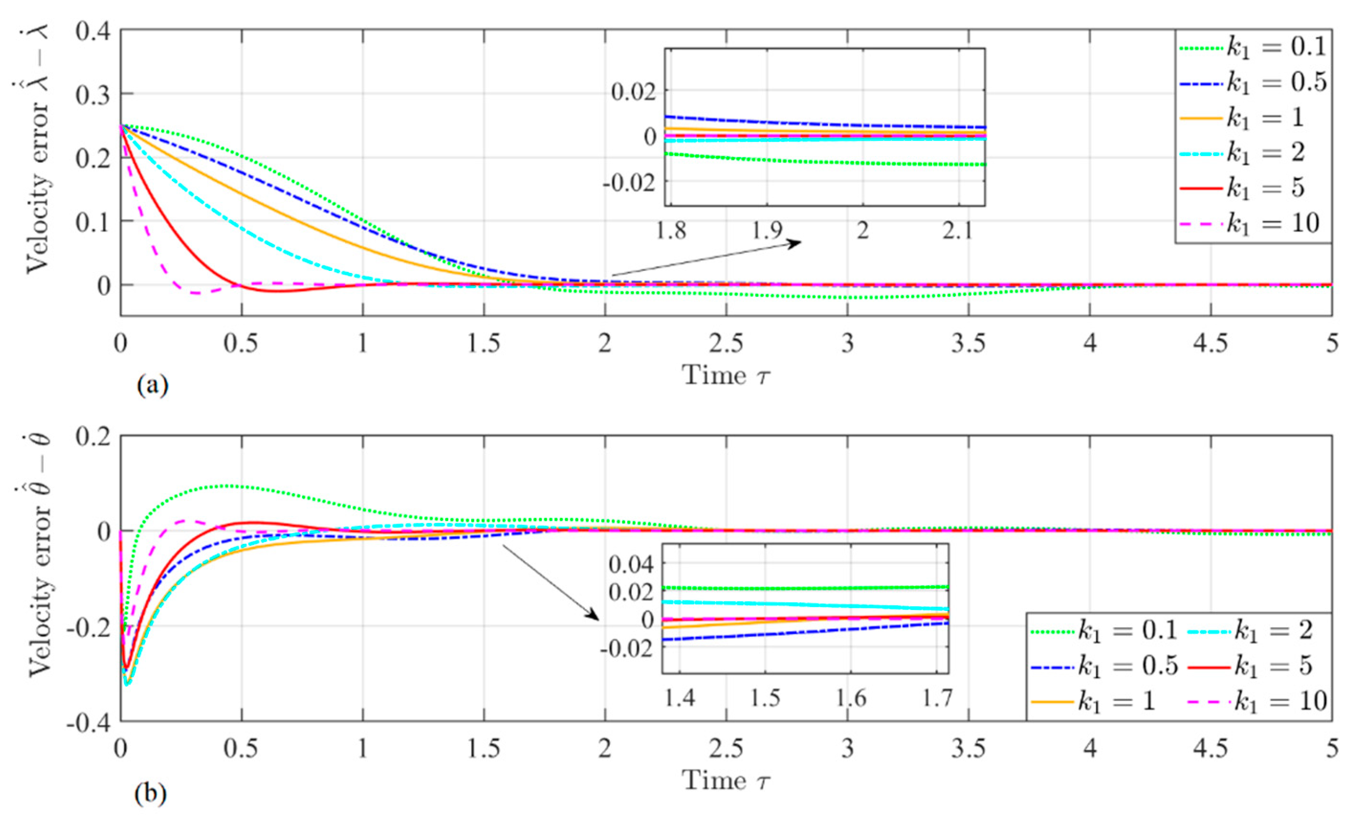
Figure 7.
Time histories of the scaling factor r.
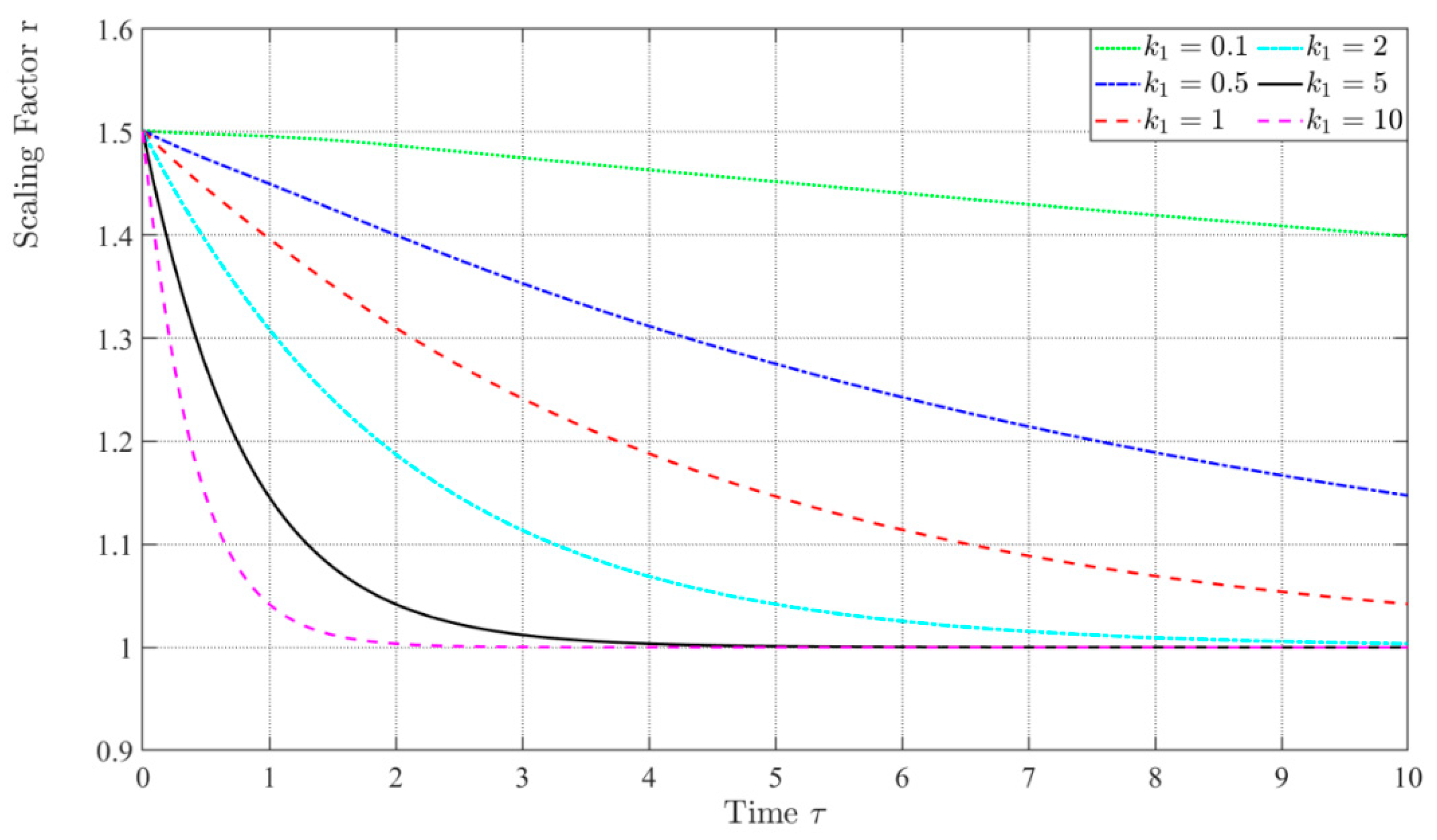
Figure 8.
Time histories of real measurement state with noise model.
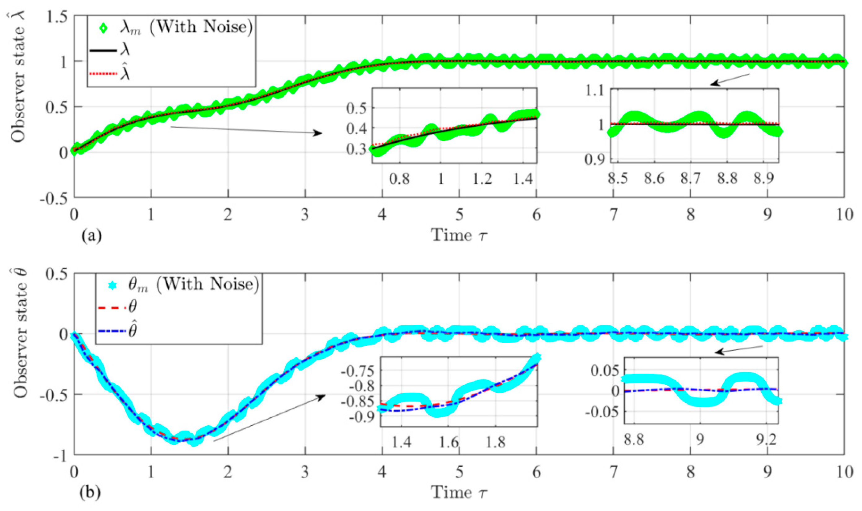
Figure 9.
Time histories of the estimated velocity with different values of the velocity gain.
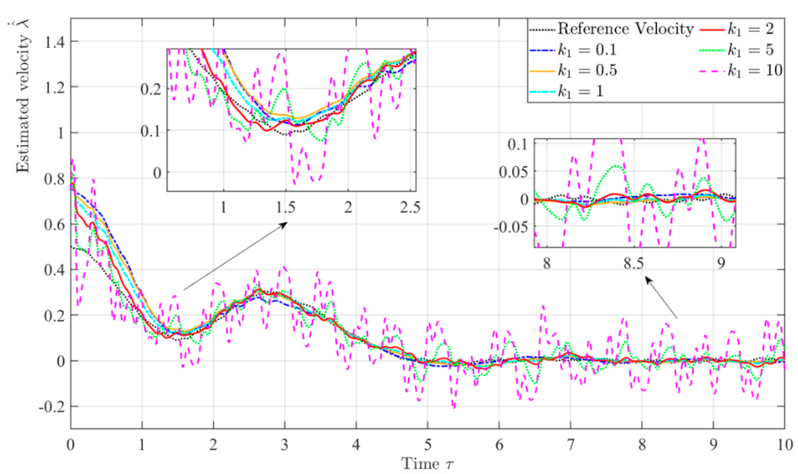
Figure 10.
Time histories of the estimated velocity with different values of the velocity gain.
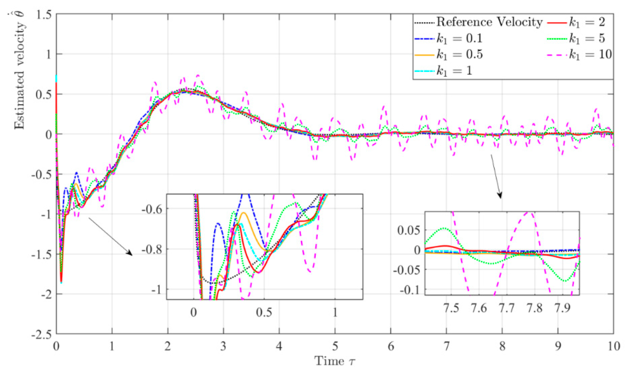
Figure 11.
Time histories of the estimated velocities and with measurement noise when the gain .
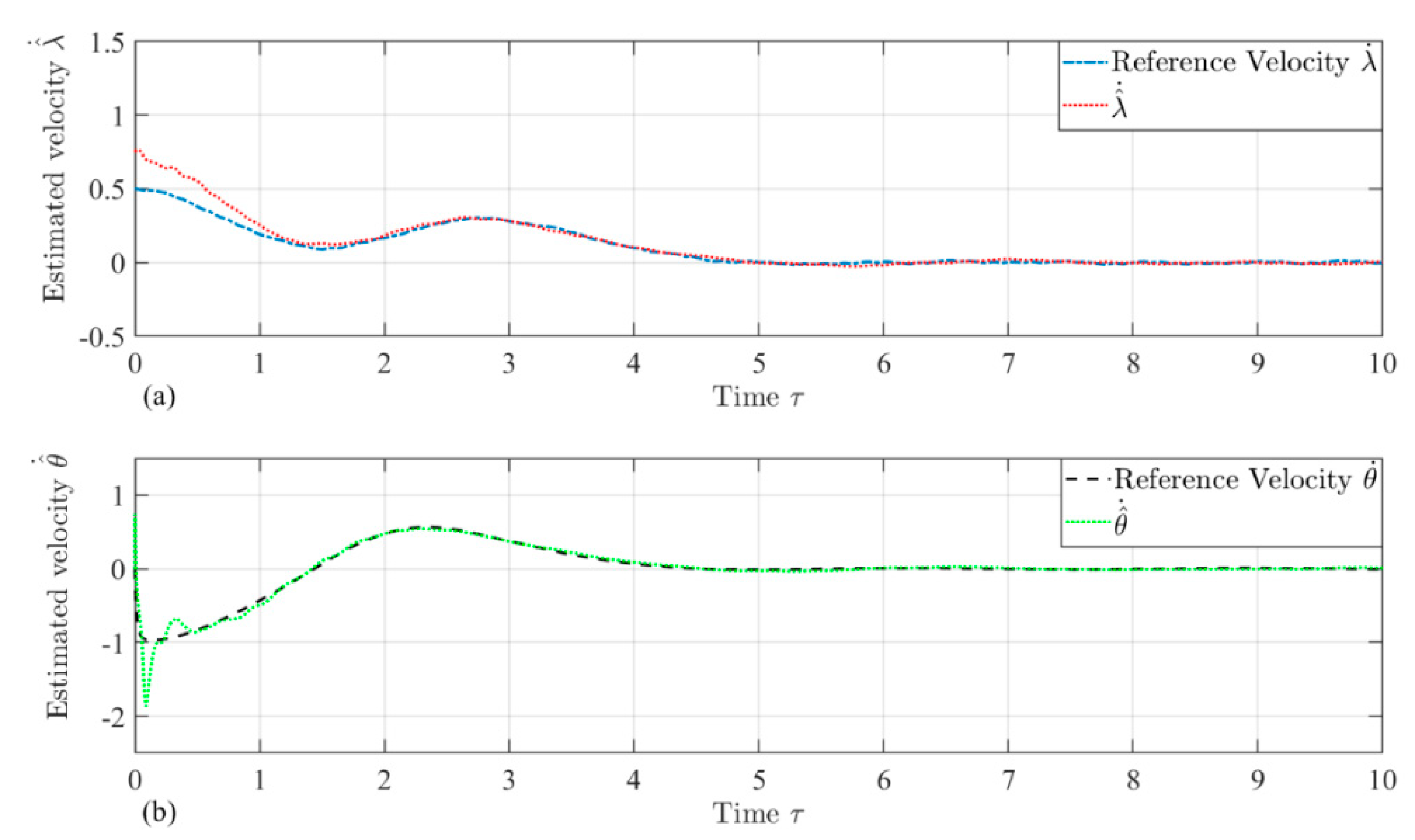
Figure 12.
Time histories of the state and of the observer dynamics at different initial velocities.
Figure 12.
Time histories of the state and of the observer dynamics at different initial velocities.
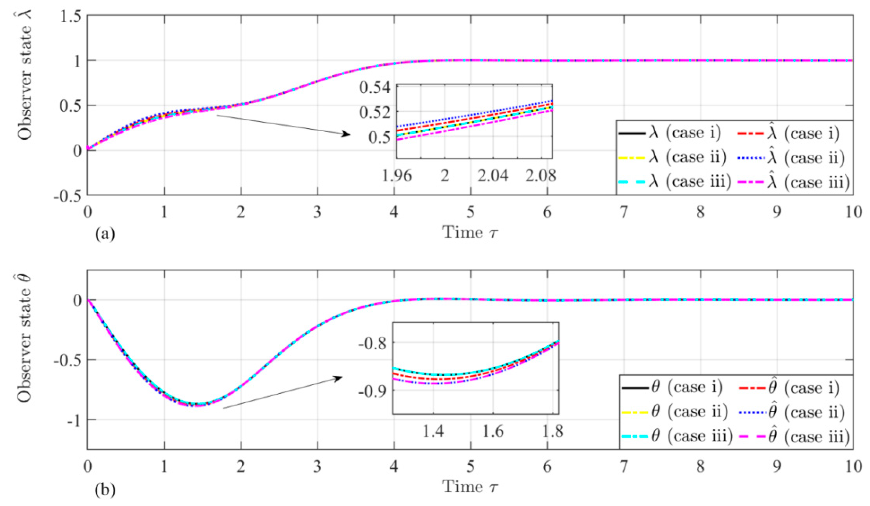
Figure 13.
Time histories of the estimated velocities and at different initial velocities.
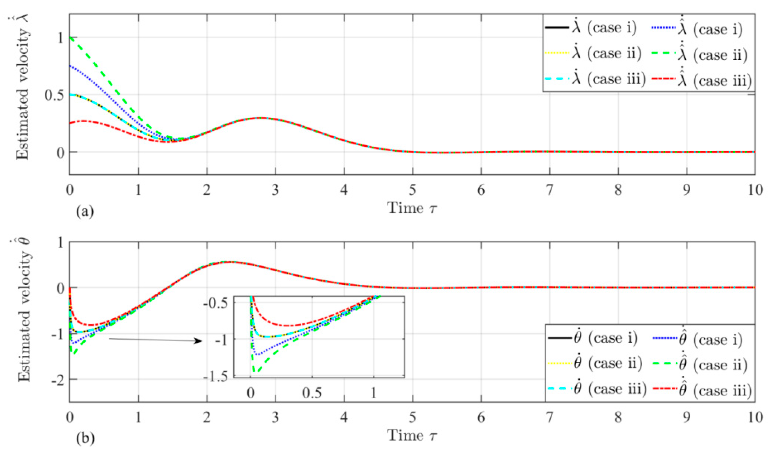
Figure 15.
Time histories of the estimated velocities and with angle rate at different initial velocities.
Figure 15.
Time histories of the estimated velocities and with angle rate at different initial velocities.
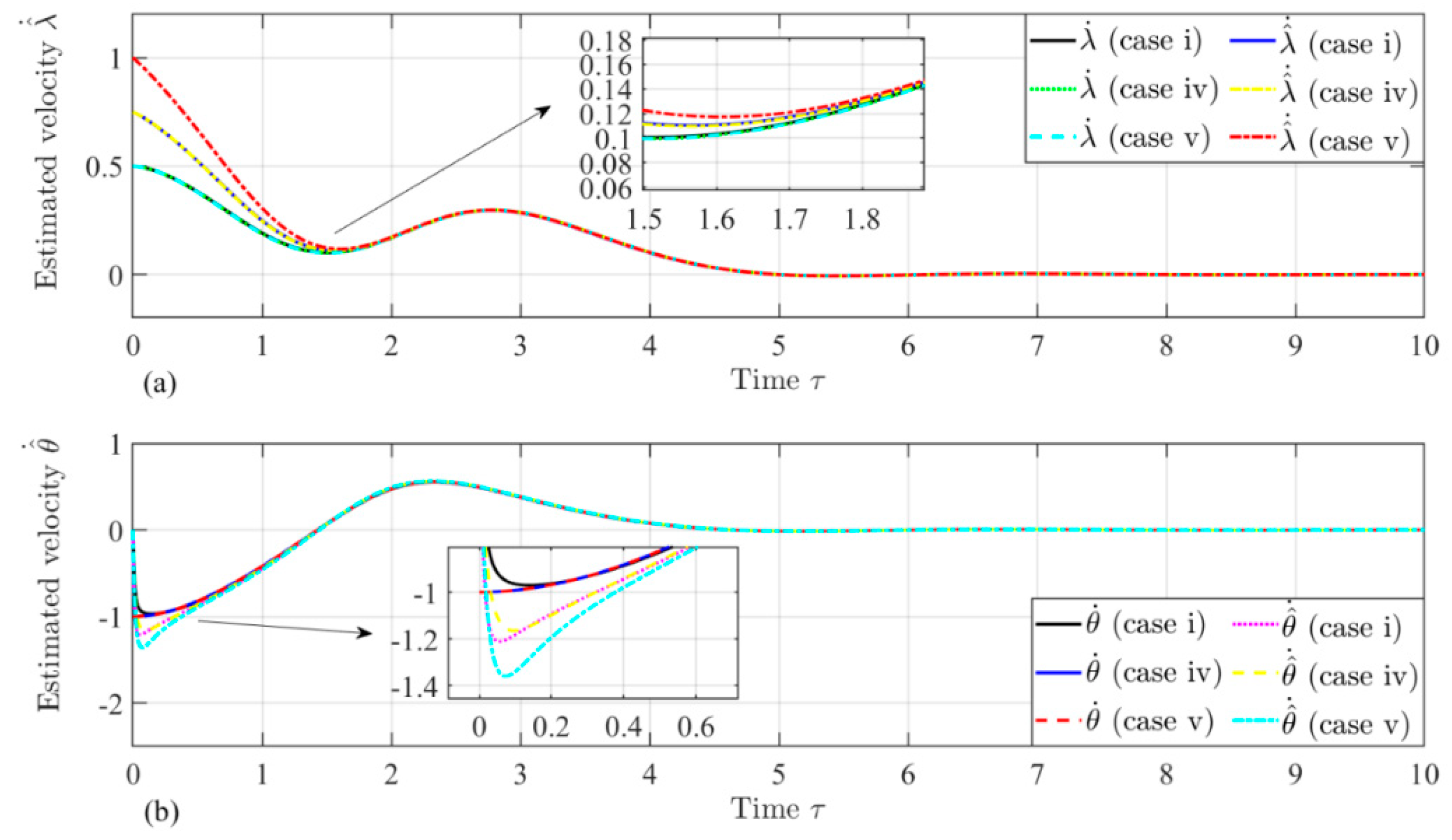

Table 1.
Simulation parameters and initial conditions for the observer dynamics.
Table 2.
Initial conditions for the observer dynamics.
| Value | ||||
| case i | 0.5 | 0 | 0.75 | 0 |
| case ii | 0.5 | 0 | 1 | 0 |
| case iii | 0.5 | 0 | 0.25 | 0 |
| case iv | 0.5 | -0.01 | 0.75 | 0 |
| case v | 0.5 | -0.01 | 1 | 0 |
Disclaimer/Publisher’s Note: The statements, opinions and data contained in all publications are solely those of the individual author(s) and contributor(s) and not of MDPI and/or the editor(s). MDPI and/or the editor(s) disclaim responsibility for any injury to people or property resulting from any ideas, methods, instructions or products referred to in the content. |
© 2024 by the authors. Licensee MDPI, Basel, Switzerland. This article is an open access article distributed under the terms and conditions of the Creative Commons Attribution (CC BY) license (http://creativecommons.org/licenses/by/4.0/).
Copyright: This open access article is published under a Creative Commons CC BY 4.0 license, which permit the free download, distribution, and reuse, provided that the author and preprint are cited in any reuse.


