1. Introduction
Optimizing energy consumption is a significant challenge for both research and industrial communities. In electric vehicles, this challenge is aggravated due to the limited capacity of batteries, which ultimately limits the range and attractiveness of EVs [
1]. Two current approaches to address this issue are the development of highly efficient powertrains and advancing energy use optimization techniques.
Regarding powertrains, one example is the use of multiple energy sources to reduce the limitation of the batteries [
2]. Supercapacitors, flywheels, and fuel cells can be combined with batteries to improve the energy management of EVs [
3,
4]. The development of highly efficient electric motors [
5] and powertrain optimization [
6] are also other approaches to reduce energy consumption. In [
7], for example, the authors present the design optimization of an in-wheel permanent magnet synchronous motor to reduce the number of materials used and weight compared to conventional motors.
The second issue addressed is energy management optimization algorithms, which offer a complementary approach to mitigating the limited capacity of batteries. In [
8], an algorithm is proposed for intelligent transportation systems, utilizing an adaptive equivalent fuel consumption minimization strategy. This approach considers the battery’s state of charge and optimizes the vehicle’s start-stop function using NARX network-based velocity prediction. This method achieved fuel savings of up to 9%. In [
9], the authors proposed a path and speed optimization strategy to extend the range of an electric unmanned marine vehicle (USV) powered by batteries and photovoltaic panels. Experimental tests demonstrated that the USV could be fully powered by PV panels under low speed and wave conditions, with path and speed optimizations increasing the range by up to 25%. Optimizing the driving profile is a crucial step in energy management. It must be tailored to the vehicle’s dynamics, weather, and road conditions to minimize energy consumption and maximize range while ensuring a minimum driving time. However, in a racing environment [
10], the vehicle consumes a significant amount of energy to achieve maximum speed over the given track distance. In this critical context, this research focuses on developing energy management strategies for implementation in a racing Formula Student prototype.
Formula Student is Europe’s most established educational engineering competition, challenging engineering students from the best universities around the world to conceptualize, design, build, and test electric or combustion single-seater formula race cars according to race car according to a specific set of rules [
11]. FST Lisboa [
12] was established in 2001 and is the Formula Student team from the University of Lisbon. Throughout its history, the team has striven to keep up with the industry’s ever-growing demands and advancements, first with the transition from combustion to electric in 2010 and then with the development of the team’s first autonomous car in 2021.
Formula Student competitions are divided into static and dynamic events. The static events assess each team’s knowledge and engineering processes. The dynamic events in the EV category include:
Acceleration: a 75m straight line to test longitudinal acceleration capability.
Skidpad: two pairs of concentric circles in a figure-eight pattern to test lateral acceleration capability.
Autocross: a single lap on a handling track with features such as hairpins, slaloms, and chicanes, approximately 1km long.
Endurance: a roughly 22km closed-loop circuit with characteristics like Autocross, including a driver change at the halfway point.
Efficiency: evaluates the vehicle’s energy efficiency during the endurance event.
Endurance and
Efficiency events together account for 325 out of 1000 points, nearly a third of the total available points. During the testing season, the team has limited opportunities to simulate endurance events, as these tests can deplete an entire battery pack or come close to it. Additionally, endurance events are the most challenging to perform consistently well in, requiring meticulous preparation in car reliability, driver training, and, most importantly, temperature and energy management. Being the most challenging event, in last year’s FSG [
13], only 13 EV teams successfully finished the Endurance (18% out of the 70 registered and 25% out of the 52 who started altogether).
The research began with the FST Lisboa team using a simple algorithm for energy management. Recognizing the lack of a robust controller to enhance overall performance in the Endurance and Efficiency events, the need for a more sophisticated system became evident, motivating this research. The ultimate objective is to develop methodologies to optimize energy use, increasing confidence in successfully completing the event and enhancing point-scoring opportunities.
We propose a methodology to generate an optimized energy reference profile and implement it in real-time. As such, a pre-event optimized plan is generated through a developed offline model and implemented into an energy management algorithm that adheres the actual energy deployment to what has been deemed optimal. The proposed methodology is validated in a real closed-loop track.
This work not only contributes to the Formula Student context but also resonates with the broader electric vehicle industry. As the industry continues its pursuit of energy-efficient solutions, this research underscores the importance of simulation-based optimization and real-time energy management.
2. Methods and Models
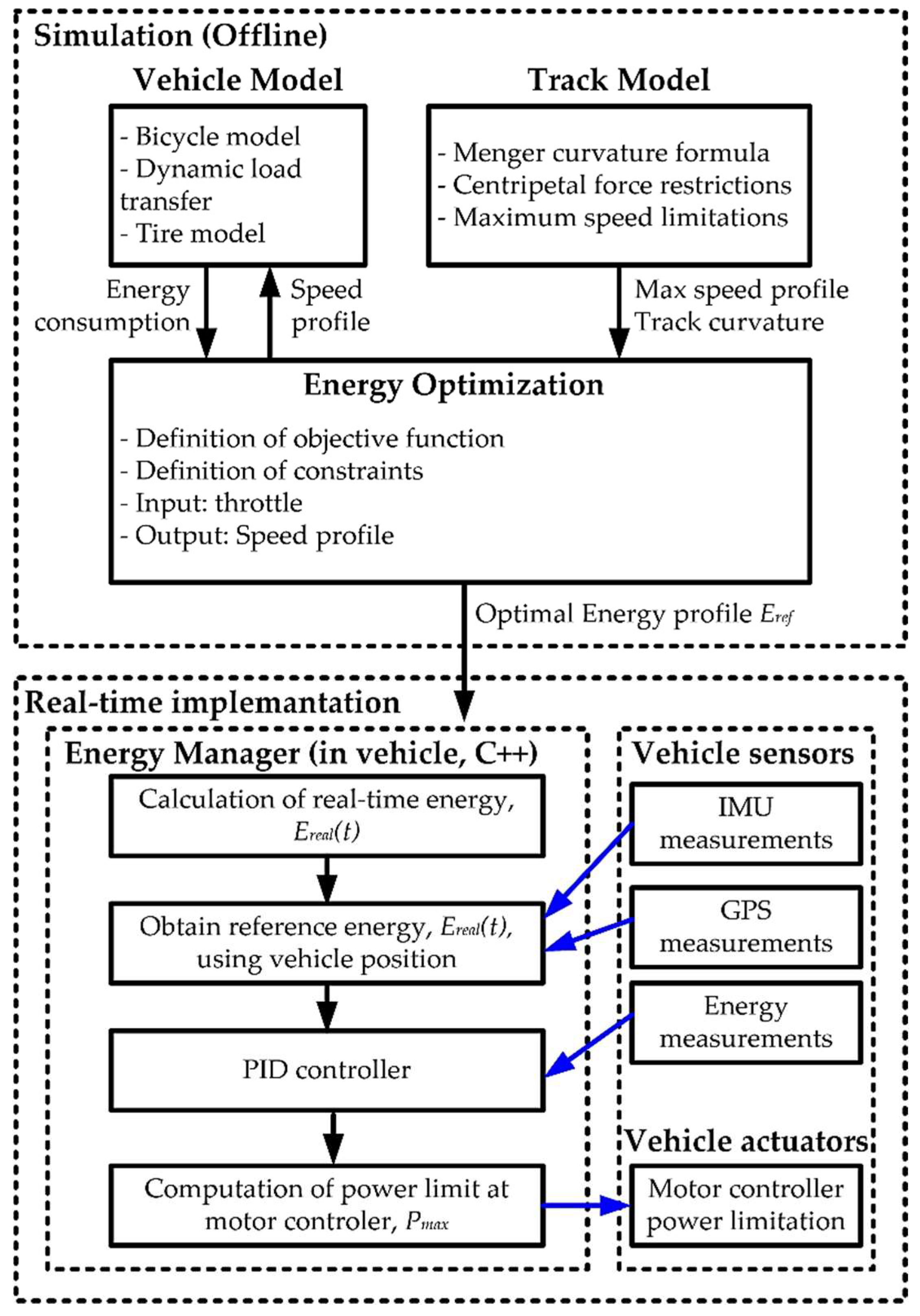
It is essential to first model the vehicle and track it to optimize energy consumption. This modeling enables the prediction of energy usage. The methodology, summarized in
Figure 1 as a flowchart, begins with defining the vehicle and track models. This step allows for an accurate estimation of the vehicle’s energy consumption under specific track conditions. Using these models, offline energy optimization is performed to refine the speed profile, aiming to maximize points in the endurance competition. Once the “optimal” speed profile is determined, it is converted to an equivalent “optimal” energy profile due to competition restrictions (remote speed control is not permitted). In real-time, an energy management algorithm estimates the energy consumption and compares it with the reference profile at the current distance traveled by the vehicle, utilizing IMU and GPS signals. A PID controller uses this error to adjust the power limitations of the motor controllers in real-time, ensuring the energy driver adheres to the optimized energy profile. Special attention is given to the distance traveled estimator, as accumulated deviations could lead to incorrect operations on the track (e.g., accelerating before a turn).
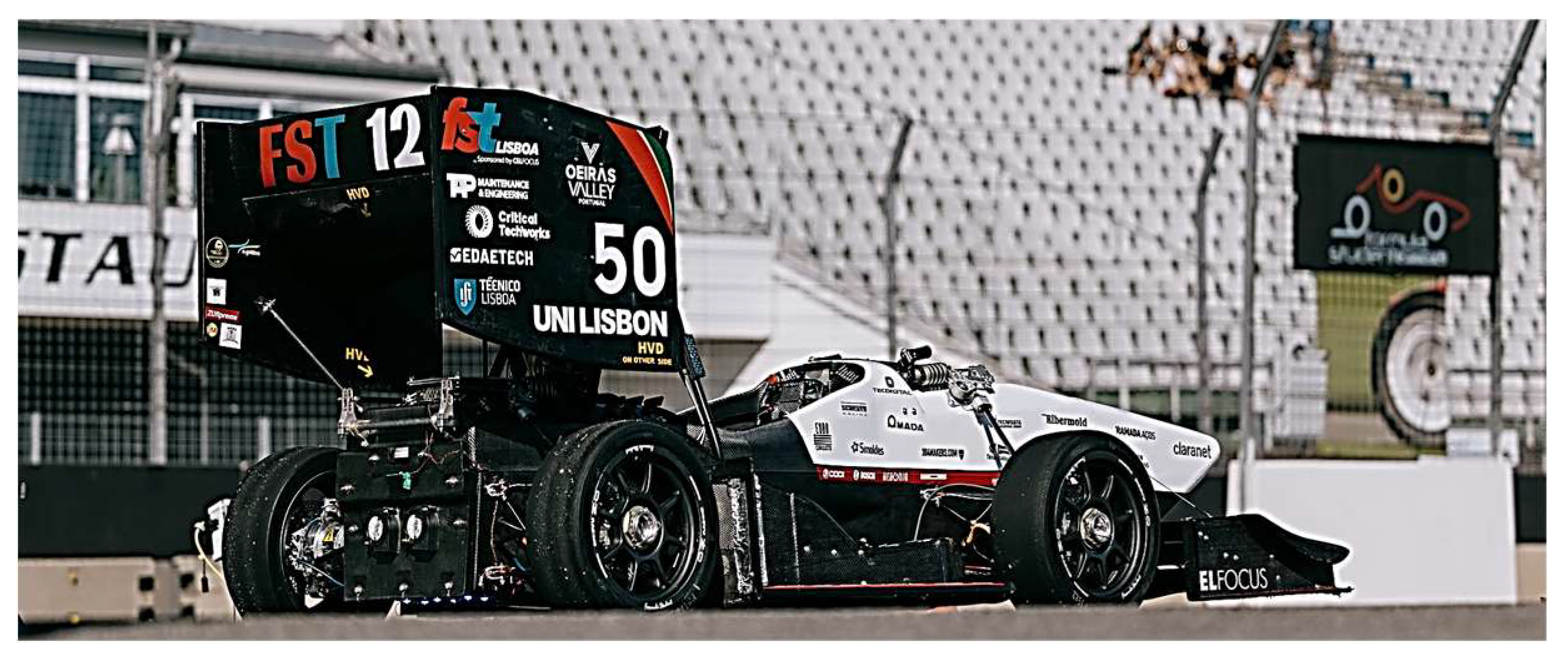
2.1. FST12 Prototype
The FST12, shown in
Figure 2, is the twelfth prototype developed by FST Lisbon. This 4-wheel drive electric vehicle features a carbon-fiber-reinforced polymer monocoque chassis, a comprehensive aerodynamic package, and a custom-built 588 V high-voltage battery. Weighing 233 kg (without the driver), the prototype boasts a power-to-weight ratio of 0.757 kW/kg. It can reach a top speed of 116 km/h and accelerate from 0 to 100 km/h in under 2.5 seconds.
Regulations limit the total power output to 80 kW in official events [
11]. The battery pack powers four 32.5 kW permanent magnet synchronous in-wheel motors, each capable of producing up to 21 Nm of torque at speeds of up to 20,000 rpm [
14]. Upon a demanded maximum power value,
Pmax, the control unit automatically distributes individual power limitations to the forward (
) and rear (
) motors as in (1).
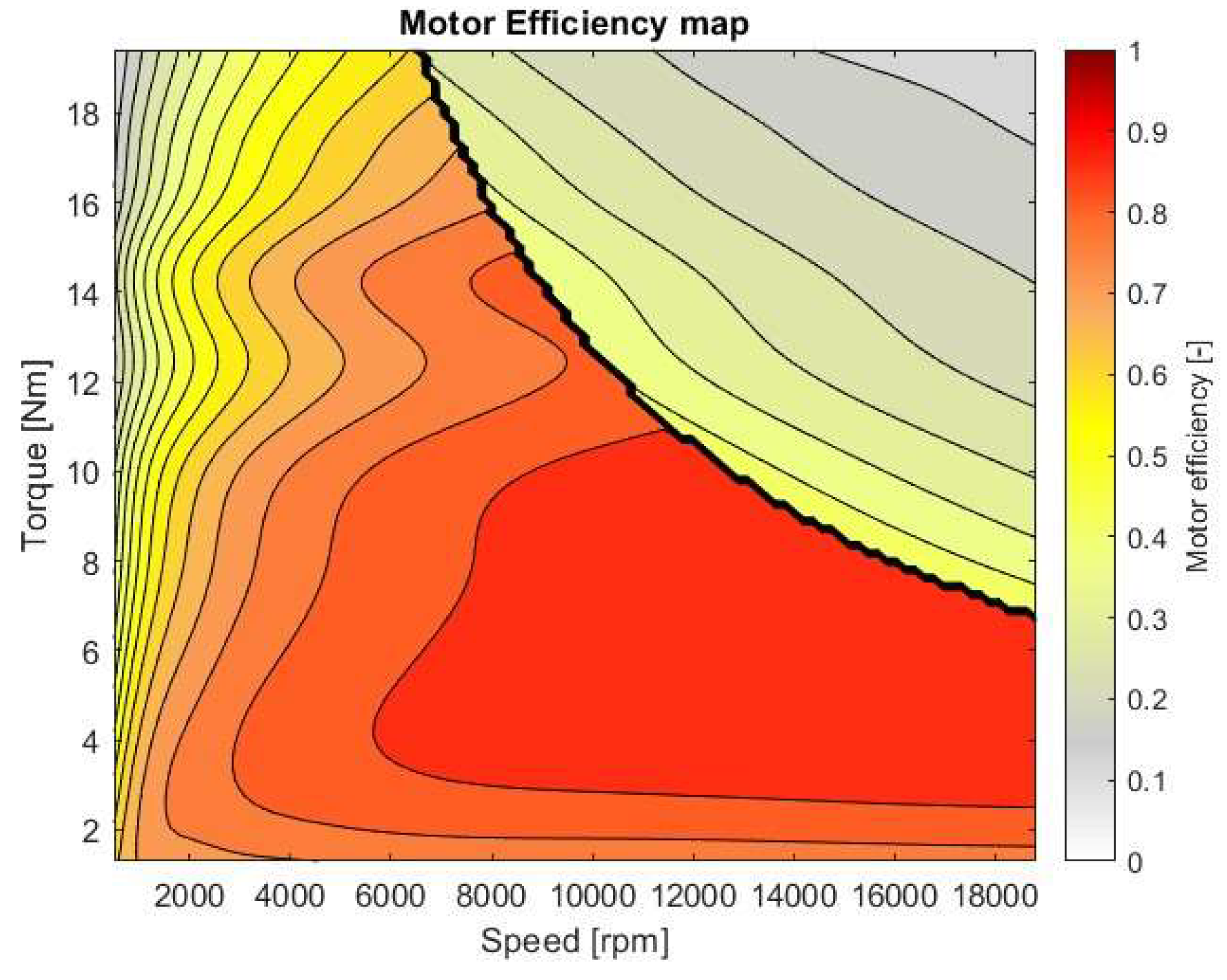
The e-motors’ manufacturer provides an efficiency map with field weakening for different operating conditions in terms of torque and speed.
Figure 3 depicts the motor efficiency map for the case of a rear motor when
Pmax = 40 kW and the maximum torque is
= 21Nm.
The battery pack comprises LiCO
2 cells, which individually have a nominal voltage of 3.7V, a charged voltage condition of 4.2V, and a typical capacity of 7.4Ah. Assembled in a 140s2p (140 series and 2 parallel) configuration, the battery pack provides a maximum voltage of 588V and a total theoretical energy capacity of 7.67kWh. While the theoretical battery capacity is 7.67kWh, the limiting value at which the vehicle can run is lower. Many factors decrease the available capacity, such as a continuous 600W low-voltage supply for various systems.
Table 1 lists the calculations one can do to estimate better the energy the fully charged battery pack can deploy.
The knowledge of the available capacity is critical for the optimization process because a small deviation can cause the energy to be drained before the track is complete. Therefore, data from previous Endurance runs helped confirm this value, as shown in
Table 2. With these results in mind, the maximum energy capacity is considered to be
Emax = 6.3 kWh.
Furthermore, the prototype is equipped with a Kvaser Memorator Pro 5xHS data logger, which allows for the post-processing of sensory data included in the CAN communication line. Using its sensor fusion algorithms, the Xsens MTi-670 GNSS/INS estimates the position, velocity, acceleration, and orientation. Integrated into the battery pack, the Isabellenhutte IVT-S-300-U3-I-CAN2-12/24 outputs voltage, current, power and energy measurements in real-time.
The prototype also incorporates a dedicated PC to handle data processing and generate torque requests directed to the inverters. This computing unit operates internal modules and communicates via a ROS/CAN protocol.
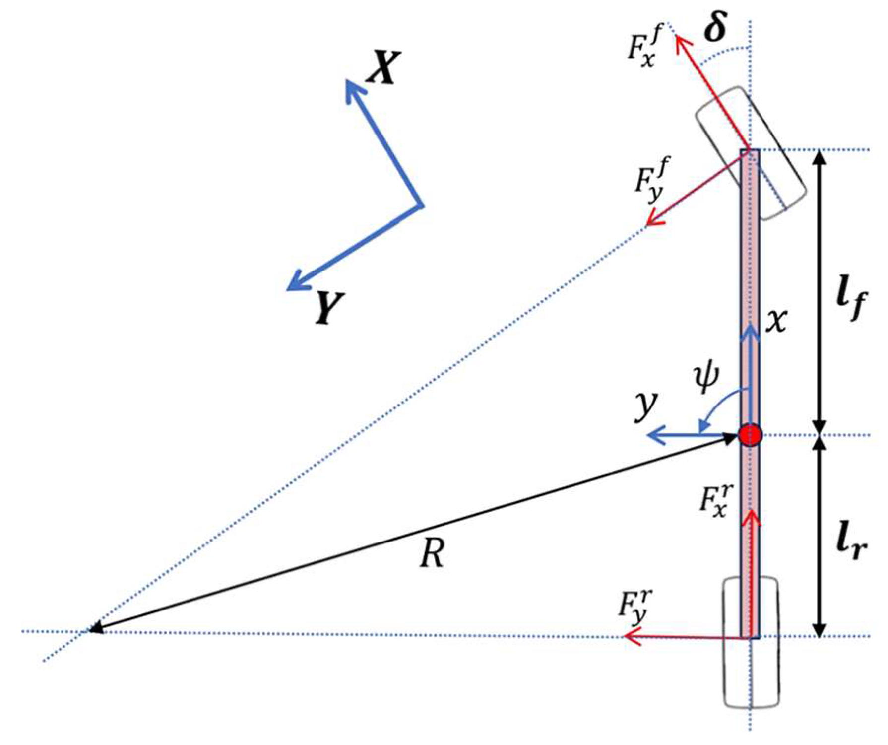
2.2. Vehicle Dynamic Model
The vehicle model built on Newtonian mechanics is based on the dynamic bicycle model described in [
15]. Its geometry can be visualized in
Figure 4. The model predicts the evolution of the vehicle state vector
x = [
X, Y, ψ, vx, vy, r]
T. Here,
X and
Y refer to the vehicle’s global position coordinates,
ψ is the vehicle’s orientation,
vx and
vy correspond to the vehicle’s longitudinal and lateral velocities, respectively, and
r is the time derivative of the vehicle’s orientation, also known as the yaw rate. The input vector contains the normalized pedal input,
p, and the wheel steering angle,
δ, described as
u = [
p,
δ]
T.
The longitudinal propulsion force provided by each of the four electric motors is given by (2), where
ηt represents the transmission’s efficiency,
GR represents the transmission’s gear ratio,
rw is the wheel’s radius,
p ∈ [−1, 1] is a normalized pedal input, and
Tmax is the programmable maximum torque value at a given motor. Additionally, the instantaneous mechanical power used to calculate energy consumption is given by the sum in all four motors (3), where
Ti and
ωi are each motor’s operating torque and angular speed, respectively. On the right side of equation (3), the wheel’s angular speed is converted into rotations per minute [rpm]. Finally,
ηpt denotes the powertrain system efficiency.
Furthermore, the grip at each tire,
FT, is estimated through individual static loads,
Fzstatic, dynamic load transfers, ∆
Fz(x or y), and downforce,
FDF, adding up to a given vertical tire load
Fz, which saturates the traction force if under the previously generated motor force (4), (5). In (4),
µx is a linear longitudinal tire coefficient and
µxs is the non-linear slope factor. In (5),
li is the tire’s axle distance to the center of gravity (
CoG), and
dfi is the downforce distribution per axle.
The dynamic load transfer calculations for the longitudinal ∆
Fzx and lateral directions ∆
Fzy are described as (6), where
m is the car’s total mass,
hcog is the height of the center of gravity,
ax and
ay are the longitudinal and lateral accelerations, respectively,
L is the wheelbase and
lw is the track dimension of the vehicle.
As such, the total longitudinal traction force of the front axle, denoted by
is the sum of the longitudinal traction forces of both front tires. The same applies to the total longitudinal traction force of the rear axle, denoted by
. In Equation (7),
Fx represents the longitudinal forces applied on the vehicle, modeled by the sum of forces around the vehicle’s CoG, such as the electric motor propulsion, rolling, and aerodynamic forces.
To define
Fy, denoting the vehicle’s lateral force, one must employ the tire slip angle
definition. This angle is defined as the difference between the wheel’s steering angle
and the wheel’s direction of travel in (8). With the tire-slip angles computed and knowing the vertical loads applied on each tire, a simplified version of the model proposed in [
16] is used to calculate the resultant lateral forces applied on each tire using (9). This application entails three coefficients to characterize the tire. Coefficient
D represents the maximum value of the lateral force for one tire,
C is a shape factor, and
B is the stiffness factor of the tire.
As such, the total lateral traction force at the front axle, denoted by
, is the sum of the lateral traction forces of both front tires. The same applies to the total longitudinal traction force of the rear axle, denoted by
. The vehicle’s total lateral force
Fy is given by (10). So, the continuous time state-space equations of the dynamic bicycle model can be consulted in Equation (11).
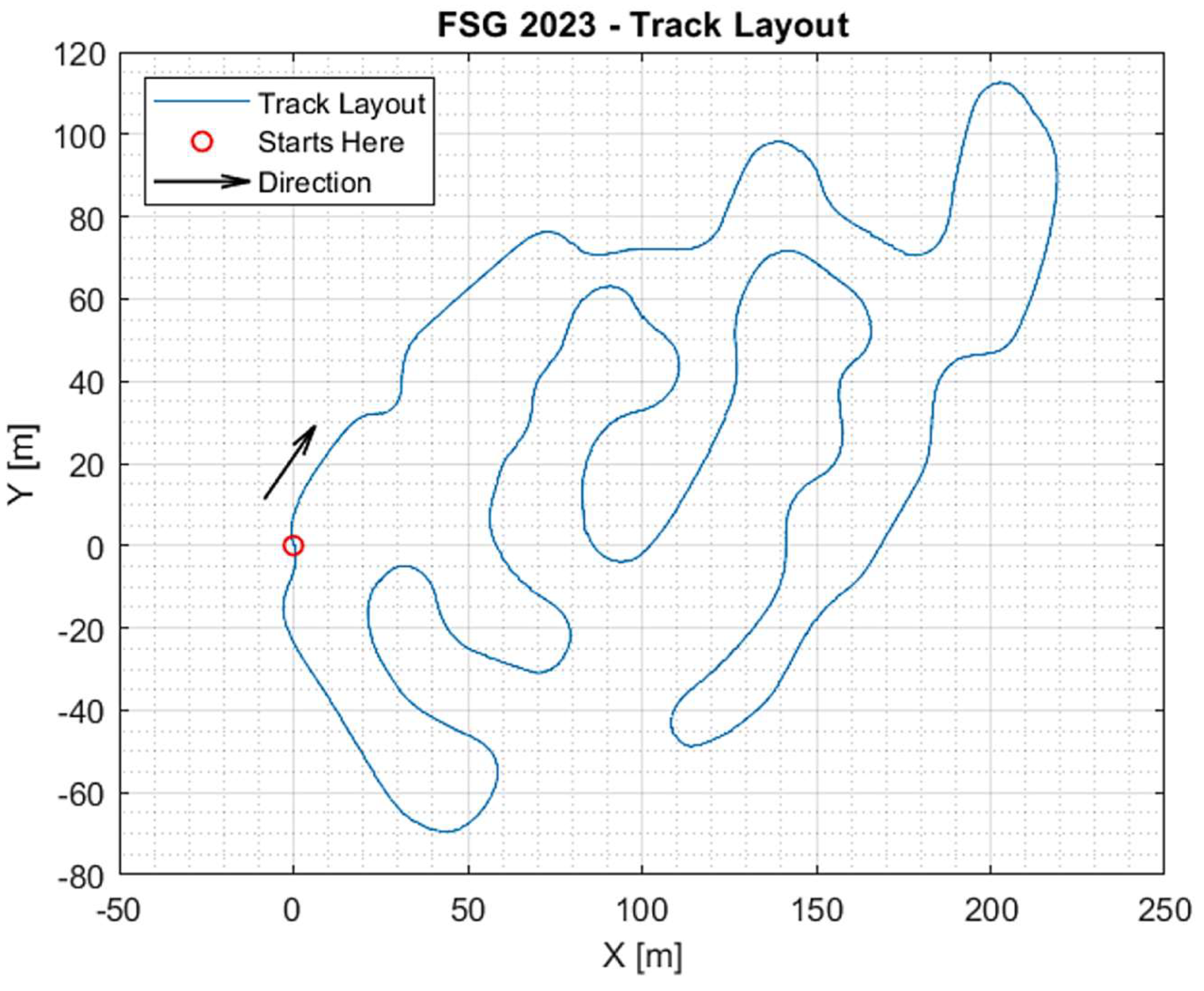
2.3. Track Model
Figure 5 illustrates the official FSG 2023 track layout (clockwise direction) obtained from GPS sensor data. The FSG competition track has a single-lap distance of 1220m. So, the competition defines the total lap number as 18 laps to complete the endurance event, which is worth roughly 22km.
In the optimization problem, each track segment is considered a variable to be optimized. As a result, the program divides each lap into different track sectors. Each is characterized by a start coordinate
Pi = (
Xi,
Yi) and an end coordinate
Pi+1 = (
Xi+1,
Yi+1), two arbitrary points in a two-dimensional Cartesian coordinate system. Derived from the Pythagorean theorem, one calculates the respective sector distance with the Euclidean formula
By discretizing the track, the vehicle dynamics must be adapted accordingly. For each step, the longitudinal velocity of the vehicle at the following step can be determined based on the current velocity and the difference in kinetic energy, as shown in (13) [
17].
Assuming that the speed is constant while running through a single track sector, the vehicle's velocity dynamic is defined by (14). Time
t is iteratively incremented by each time interval needed for the car to cross each segment
, as shown in (15).
The vehicle's lap time,
Tteam, relates to the last value of
tN, which is the accumulated run time after the total number of track sectors,
N. Each segment's energy is computed by multiplying the instantaneous mechanical power (3) with the sector time
. The vehicle's total consumed energy,
Eteam, is calculated as (16) by accumulating all
N sector values and conversion to [kWh].
Physically, the car's velocity at each sector is limited by its maximum velocity,
vtop, or the maximum allowed centripetal force
. This is expressed in (17), where
vtop is the vehicle's top speed,
R is the turn radius,
D is a tire coefficient that refers to the maximum lateral force in each tire and
m is the vehicle's mass.
Moreover,
R can be obtained through an iterative implementation of the Menger curvature [
18] formula. Given the Cartesian coordinates of three sequential points (
x,
y,
z), the curvature
C and subsequent turn radius
R are calculated as (18) and (19), where
A denotes the area of the triangle spanned by
x,
y and
z.
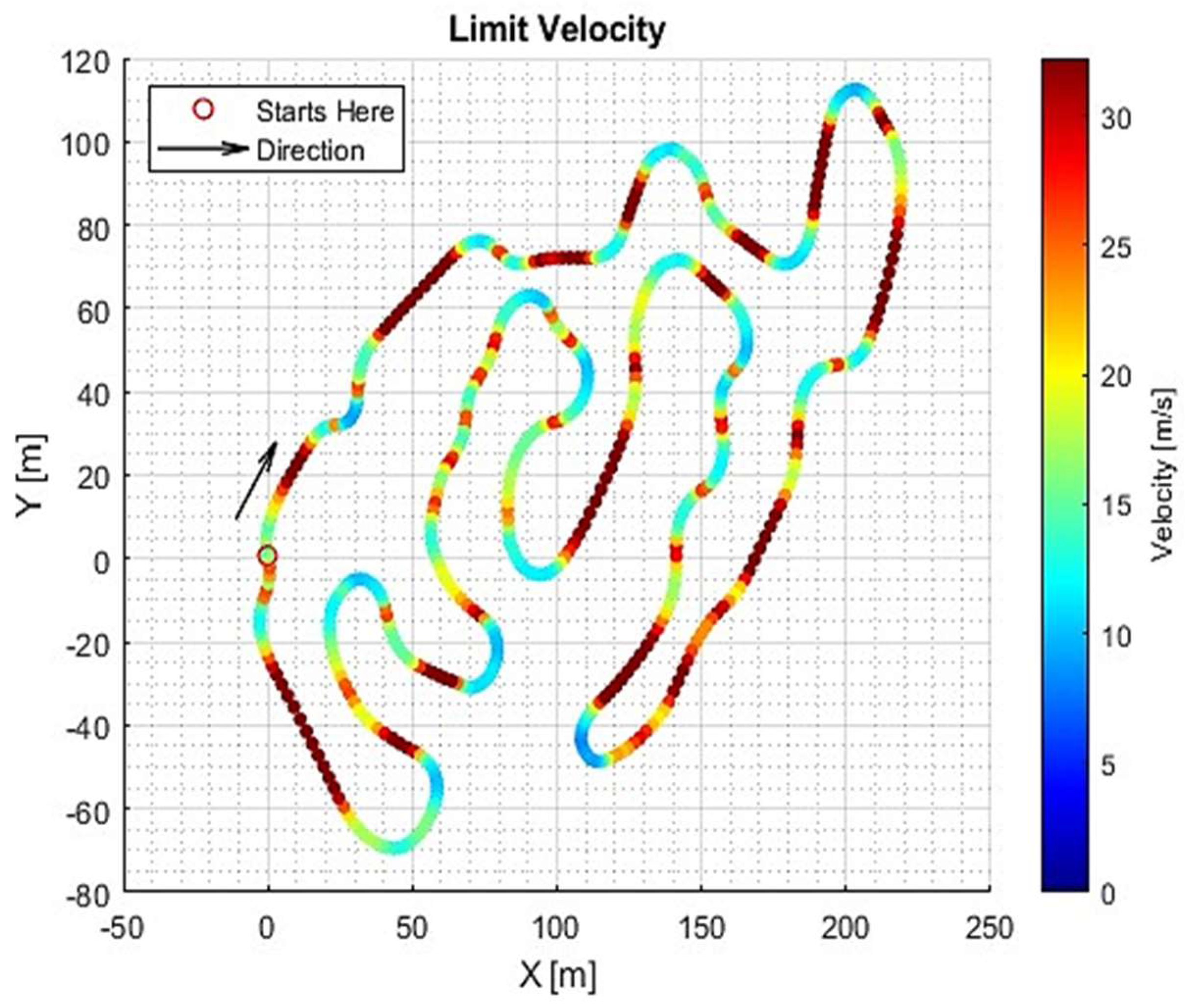
Note that when the track’s center line is straight, the curvature (18) tends to zero and the radius (19) tends to infinity. In this case, the vehicle’s maximum achievable velocity
vmax (17), is its maximum straight-line velocity,
vtop. Otherwise, its velocity will be limited by the maximum allowable lateral centripetal force, which depends on the vehicle’s mass and tire parameters.
Figure 6 depicts the resultant velocity limit values along one lap of the track.
Lastly, the steering angle
δ required for the vehicle to follow the track can be determined using (20), where
L and
lw are the vehicle’s wheelbase and track width, respectively.
Note that the above steering angle obtained from GPS data does not necessarily correspond to the track’s centerline. Instead, it reflects the driver’s chosen racing line, known for being more efficient in terms of speed and energy saving.
2.4. Distance Estimation
To ensure that the energy reference set-point is accurately aligned with the distance traveled, it is imperative to establish a dependable and precise method for odometry calculation. Given the available sensors and also the preliminary results using offline simulations with logged data, the methodology chosen for continuous distance estimation during the Endurance run was inertial odometry. This estimates a vehicle’s position based on measurements from inertial sensors, typically accelerometers and gyroscopes.
2.5. Optimization Problem
The ultimate goal of the optimization problem is to solve for the maximum points in the sum of the Endurance and Efficiency scoring. According to FSG’s rules [
11], the score for the Endurance event is calculated with (21), 25 points for finishing, and a maximum of 225 points attributed to how fast the car finishes the event, normalized to the fastest car, where
Tteam is the team’s corrected elapsed time, and
Tmax is 1.333 times the corrected elapsed time of the fastest vehicle.
Moreover, the Efficiency score is calculated with (22), where a maximum of 75 points is awarded to a team depending on its efficiency factor in comparison to other teams, where
EFmin is the lowest (best) efficiency factor of all teams,
EFmax is defined as 1.5
EFmin, and
EFteam is the team’s efficiency factor, given by equation (23), where
T is the uncorrected elapsed driving time, and
E is the energy used.
The results from the most recent competition, FSG23, published at [
13], are listed in
Table 3.
To maximize the score, considering the vehicle’s powertrain limitations to finish the event plus physical constraints, the cost function prioritizes point scoring according to (21) and (22), aiming to strike a balance between lap-time performance and energy consumption. The optimization problem is defined as follows (24), where the cost function is minimized concerning the pedal’s input state,
u =
p, and
λi are soft constraint’s weights, allowing control over two crucial soft constraints.
At each sector, the vehicle cannot exceed a maximum velocity, which is either limited by the maximum allowed centripetal force or the vehicle’s maximum velocity (25). Also, the vehicle must not exceed the maximum energy capacity of the battery pack as, in the real event, it would result in a DNF (Did-Not-Finished), scoring zero points (26).
Regarding the control input,
u =
p, there are two inequality constraints, which, algebraically written, are given by the following matrices:
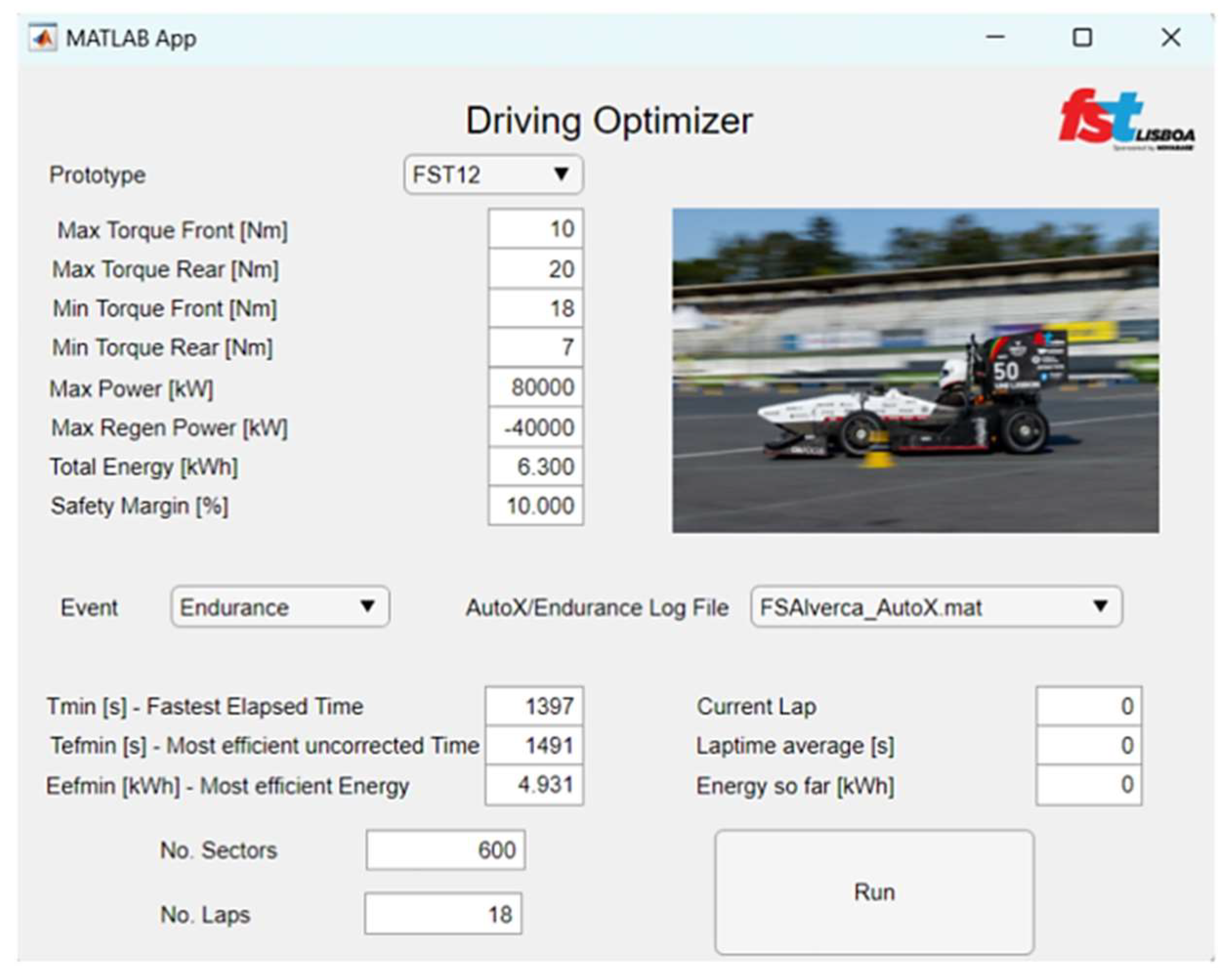
A simulator was developed in
MATLAB to run the optimization environment,
Figure 7. It starts by initializing an app interface that asks the user to input the track layout, vehicle physical and powertrain parameters, and optimization parameters. After discretizing the track environment, the program simulates multiple iterations of the Endurance event using the appropriate vehicle model while optimizing the control vector with the cost function (24) to maximize the score in both Endurance and Efficiency events. For this purpose, the
MATLAB optimizing function
fmincon is used to find the optimal solution given the constraints or a limit of iterations. After reaching the optimal solution, an output file containing the optimized energy reference line in function of the distance is generated.
2.6. Controller Implementation
2.6.1. Endurance Energy Manager
The system takes an optimal energy reference line in function of distance as its input and continually adapts the vehicle’s maximum power constraint, denoted as
Pmax. Given the endurance distance status, this adjustment depends on whether the current energy level exceeds or falls short of the expected energy level. An error (28) is computed between the current energy level and the referenced set-point. This depends on continuous distance estimation,
d, along the Endurance.
Then, the new vehicle’s maximum power (29),
Pmax, is computed using a simple PI-Controller on the error resultant from (28) to compute the power limit adjustment that is then added/subtracted onto the initial power limiting value,
Pinit. In (29),
Kp and
Ki are controller gains, proportional and integral, respectively. These gains are used to tune the aggressiveness of the power limit adjustments.
2.6.2. Distance Estimation Methodology
The results of running offline simulations with this measure on different endurance log samples are shown in
Table 4. As can be seen, the differences between the estimated distances and the actual ones are very close, with a deviation of less than 0.7%.
2.6.3. Distance Estimation Methodology
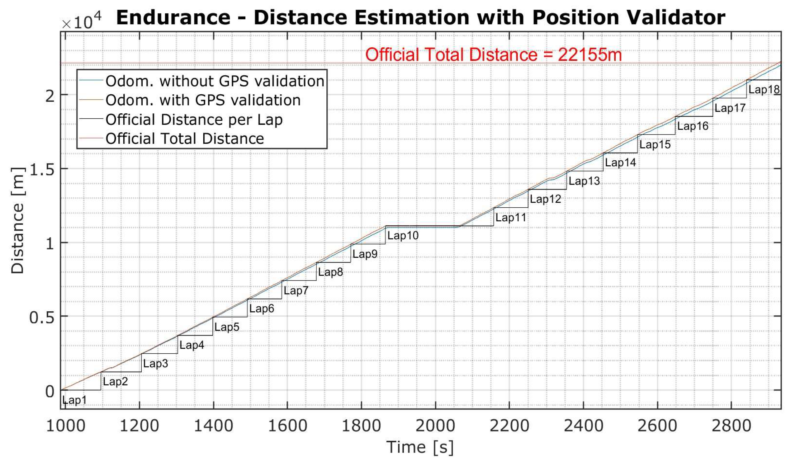
However precise, the methodology above remains susceptible to error accumulation along the lengthy Endurance event. To address this challenge, a new system was introduced. The position validator operates by continuously monitoring distance estimates derived from inertial odometry, aligning them with expected positions on the track layout. It then validates the distance estimate by performing real-time cross-validation with the GPS outputs. The algorithm compares the expected track position with the actual GPS-derived position, computing the Euclidean distance and checking if it falls within an acceptable threshold. The threshold is expressed as a maximum radius around the expected point, Rmax. In cases where the distance discrepancy exceeds this threshold (∆d > Rmax), indicating error accumulation over what is deemed acceptable, the system dynamically corrects the distance using GPS data and adjusts for the elapsed number of laps.
Using logged data from the most recent Endurance event (FSG23), with the maximum acceptable discrepancy defined at
Rmax = 5 m, the
position validator eliminates the accumulated residual error of the
inertial odometry worth over 140 meters, as seen in
Figure 8.
2.6.4. Pipeline Implementation
The controller now implemented relates to the Endurance Energy Manager, who dynamically adjusts the vehicle’s power limitation to ensure that the vehicle closely adheres to the pre-established optimal energy reference line. Like the rest of the pipeline, the module is programmed in its own SIMULINK model, incorporating MATLAB functions. After being tested offline, the code was generated in C++ using the SIMULINK Coder built-in feature, and the target file was set appropriately. A working frequency of 10 Hz was chosen for the Endurance Energy Manager module. Finally, the C++-generated code is implemented on the team’s ROS/CAN communication pipeline. New signals were added to the CAN line, and the appropriate signal/module connections were made in the ROS communication pipeline. The module’s inputs are:
IMU: 3x1 vector containing IMU readings (vx,vy,ψ).
GPS: 2x1 vector containing GPS readings (latitude, longitude).
isaenergy: accumulated energy value, in Wh.
EMenable: Turns the controller module ”on/off”.
maxpwr: Limits total power as a safety measure, in W.
initPL: Algorithm’s initial power limiting value, in W.
EMkp: Controller’s proportional gain.
EMki: Controller’s integral gain.
dprev: Discretely accumulated distance value, in m.
The outputs are:
EMpwrlimit: Energy Manager algorithm Pmax computation, in W.
pwrlimit: Sent to the Power Limiter;
d: Accumulated distance run by the vehicle.
eref: Current energy reference setpoint, Eref(d).
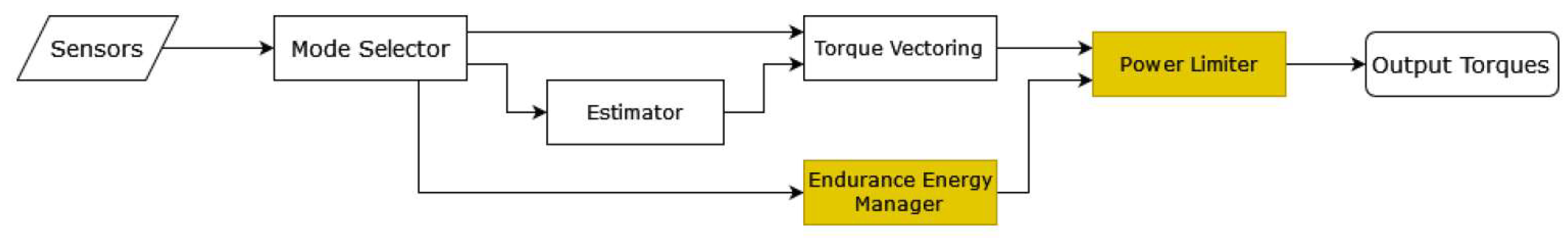
Figure 9.
Control system pipeline implementation.
Figure 9.
Control system pipeline implementation.
3. Results
3.1. Model Mismatch
Prior to the optimization, it is important to test the developed models and compare the outputs to real measurements, using the same inputs to try and validate outputs. Thus, the models were developed in
SIMULINK and fed with real logged driving data regarding the fastest FSG Endurance event lap as input.
Table 5 shows the mean-squared error results for velocity and energy outputs obtained by sensors compared to their reference.
In light of these results, due to its closer representation of the real prototype in racing conditions, the chosen model is the dynamic bicycle model. Additionally, the optimization process entails multiple iterations, each characterized by its runtime, influenced by model complexity and the number of variables (sectors). Due to extended runtimes in SIMULINK for each iteration, it is necessary to discretize the process in MATLAB. This has been executed, and Table 6 lists the results.
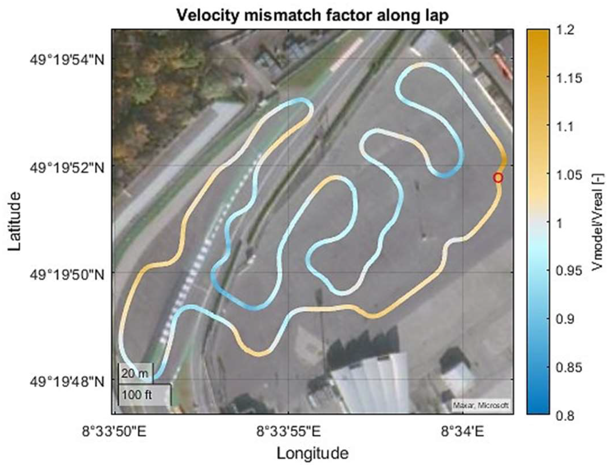
To observe where the model is missing most,
Figure 10 represents a velocity mismatch percentage factor along the track layout given by
V/
Vreal. This computes values over 1 when the model estimates the vehicle driving faster than in reality and values under 1 when estimating a lower velocity.
Predominantly, there is a slight overestimation (yellow) of the vehicle’s velocity in straights and an underestimation (blue) in most tight corners. The effectiveness of the multivariable optimization process is significantly impacted by the number of variables represented by track partitions in this context. This influence extends to both model accuracy and computational speed. Upon evaluating the results for vehicle velocity mismatch (in MSE) and lap simulation duration while altering the total number of partitions in a single lap, a noteworthy conclusion emerges: Beyond 3000 lap sectors, there is marginal improvement in terms of model accuracy, while the single iteration time steadily increases linearly. This has substantial implications for optimization time, particularly when the process involves computing thousands of iterations to identify the optimal solution.
3.2. Optimization Results
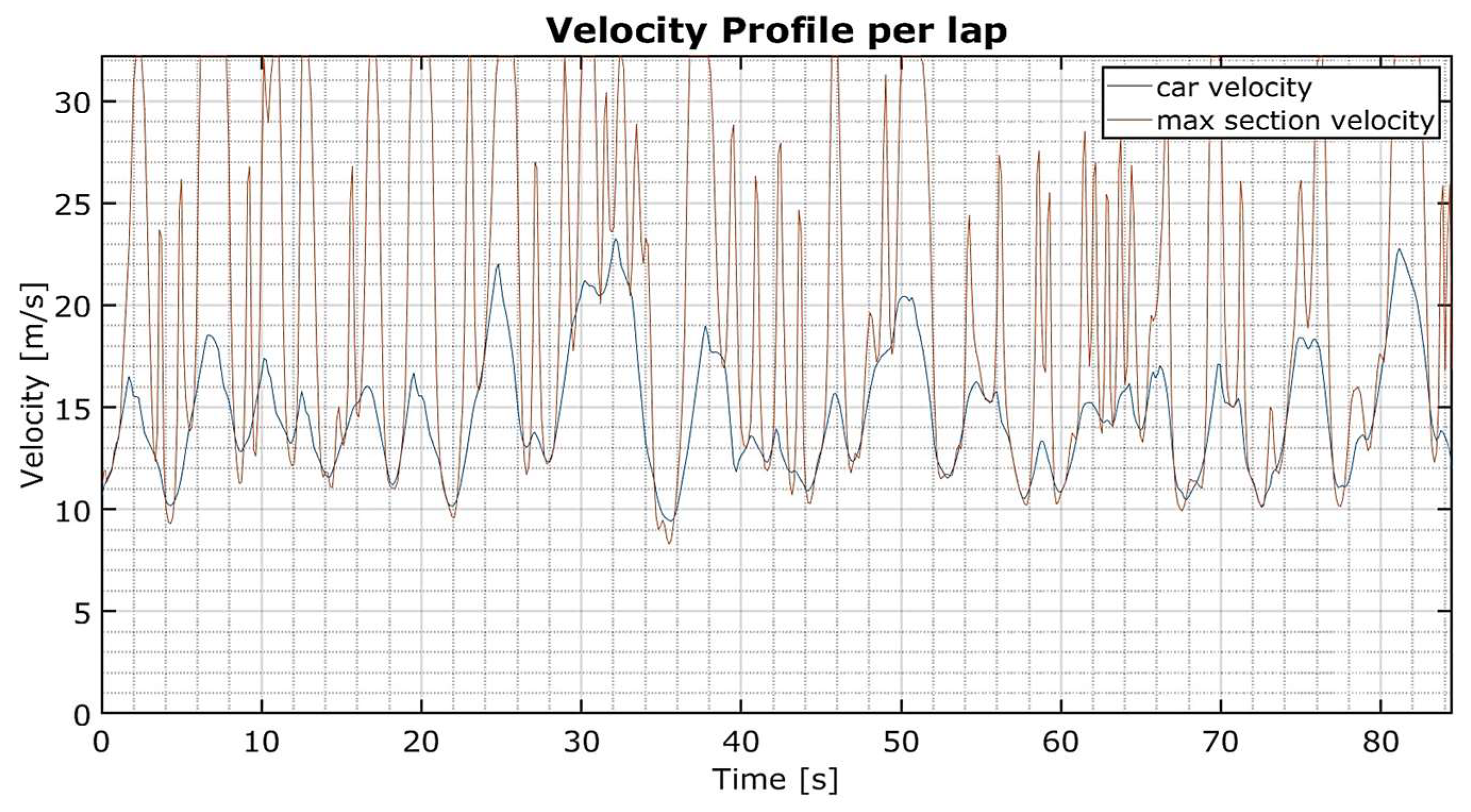
In the Endurance event, the focus lies on lap time optimization and energy consumption. The balance is modeled in the cost function (24). The objective is to achieve the highest joint score while ensuring the car completes the 22 km distance within its maximum energy capacity and physical limitations. Running the optimization of the
FST12 prototype around an 18-lap Endurance event on the official 2023 FSG track layout (see
Figure 5), the resulting velocity profile along time is shown in
Figure 11. Additionally, it is compared to the maximum velocity in each track section, as defined in equation (17).
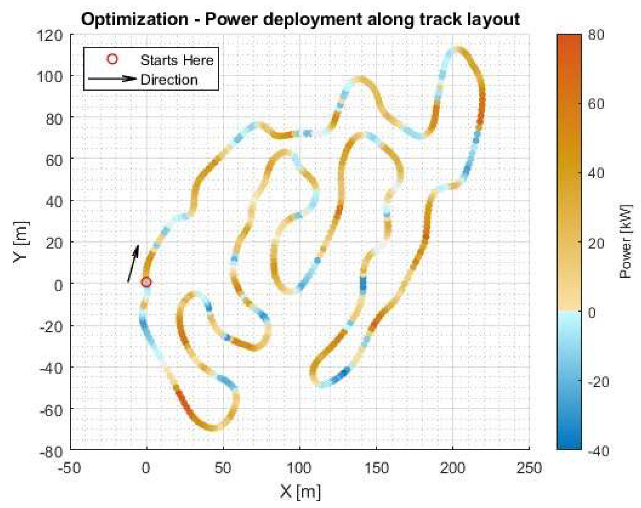
Figure 12 shows the resulting power deployment along the lap.
As one can observe, the optimization sees the vehicle matching maximum corner speeds for lap time reduction and manages energy in the two main straights (especially), easing off the throttle and even regenerating slightly (see
Figure 12).
In summary, the
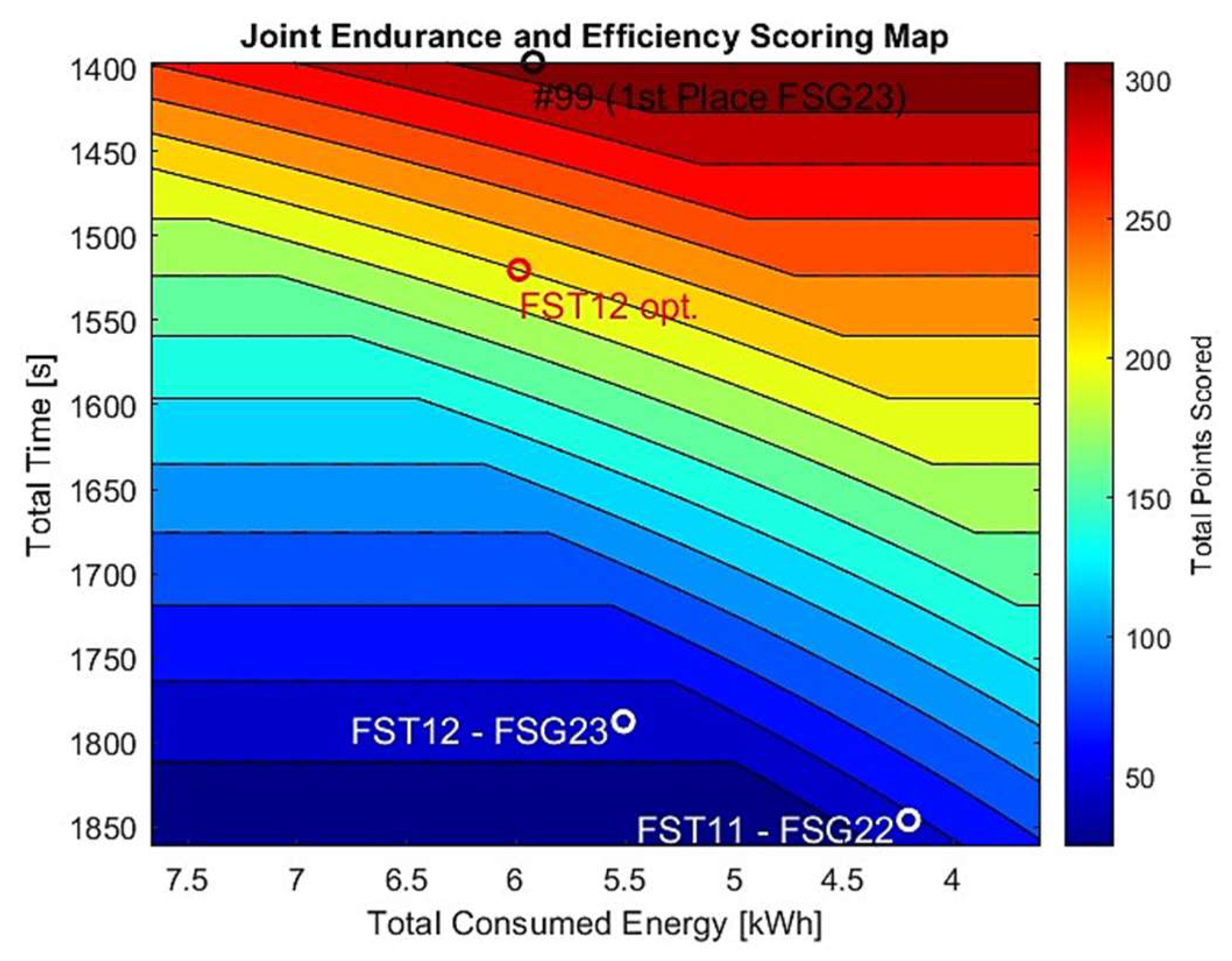
FST12 completes the simulated FSG Endurance event with a total elapsed time of 1520 seconds, consuming a total energy of 5.985 kWh (out of 6.3kWh), showing it is not optimal to consume all available energy for maximum points. As a result, the average lap time is 84.44 seconds, with an energy consumption of 0.333 kWh per lap, which would result in 177 points and an additional 35.7 points for efficiency, bringing the total to 212.7 points out of 325, as illustrated in
Figure 13. Also, this figure shows the real points obtained in the competitions of 2022 (FST11-FSG22) and 2023 (FST12-FSG23) by the FST team without energy optimization. This optimization process can achieve a high increase without changing the vehicle’s performance and structure.
3.3. On-Track Results
For the test run, the routine expected in competitions was performed on a real track in Alverca, Portugal. The practical plan for using the system involves first optimizing the Endurance profile based on the track data gathered during the Autocross event (held a day before Endurance). Afterward, the optimized plan is uploaded to the car’s control unit, and the energy monitoring system is enabled to run throughout the event. Given the absence of other teams for competitive benchmarks on the final test run day and the inability to fully recreate one of the already existing layouts, a better team was assumed to be 5% faster and 15% more efficient than a representative Autocross lap set by the
FST12 around the track in question. So, the driver performed a total of 4 laps, and the average lap time was 72 seconds with an average energy consumption of 0.26 kWh per lap. The chosen track has a lap distance of 884 meters, adhering to FS layout regulations [
13], and the run programmed in this test consists of 22 laps around the circuit below.
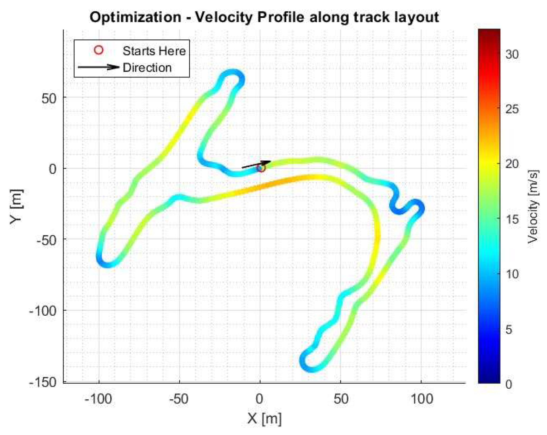
After the initial Autocross runs, the battery pack was charged back up to nearly 95%. In the meantime, the track data was extracted and the offline optimization was performed. The result for the velocity profile around the layout can be consulted in
Figure 14.
Overall, the FST12 completed the simulated event with a total elapsed time of 1522.1 seconds, consuming a total energy of 5.355 kWh. The average lap time is 70.55 seconds, with an energy consumption of 0.243 kWh per lap, resulting in 222.6 points for the Endurance event and an additional 49.2 points for efficiency, bringing the total to 271.8 points out of 325. Having concluded the optimization, the resulting energy plan was uploaded to the car’s control unit’s energy management system and the Endurance run was begun.
In reality, the
FST12 completed the full
Alverca Endurance run in 1574.6 seconds, consuming a total energy of 5.383 kWh. A video onboard of one of the Endurance laps can be found through the QR code depicted in
Figure 15. Compared to the optimization-based simulation, the results are presented in
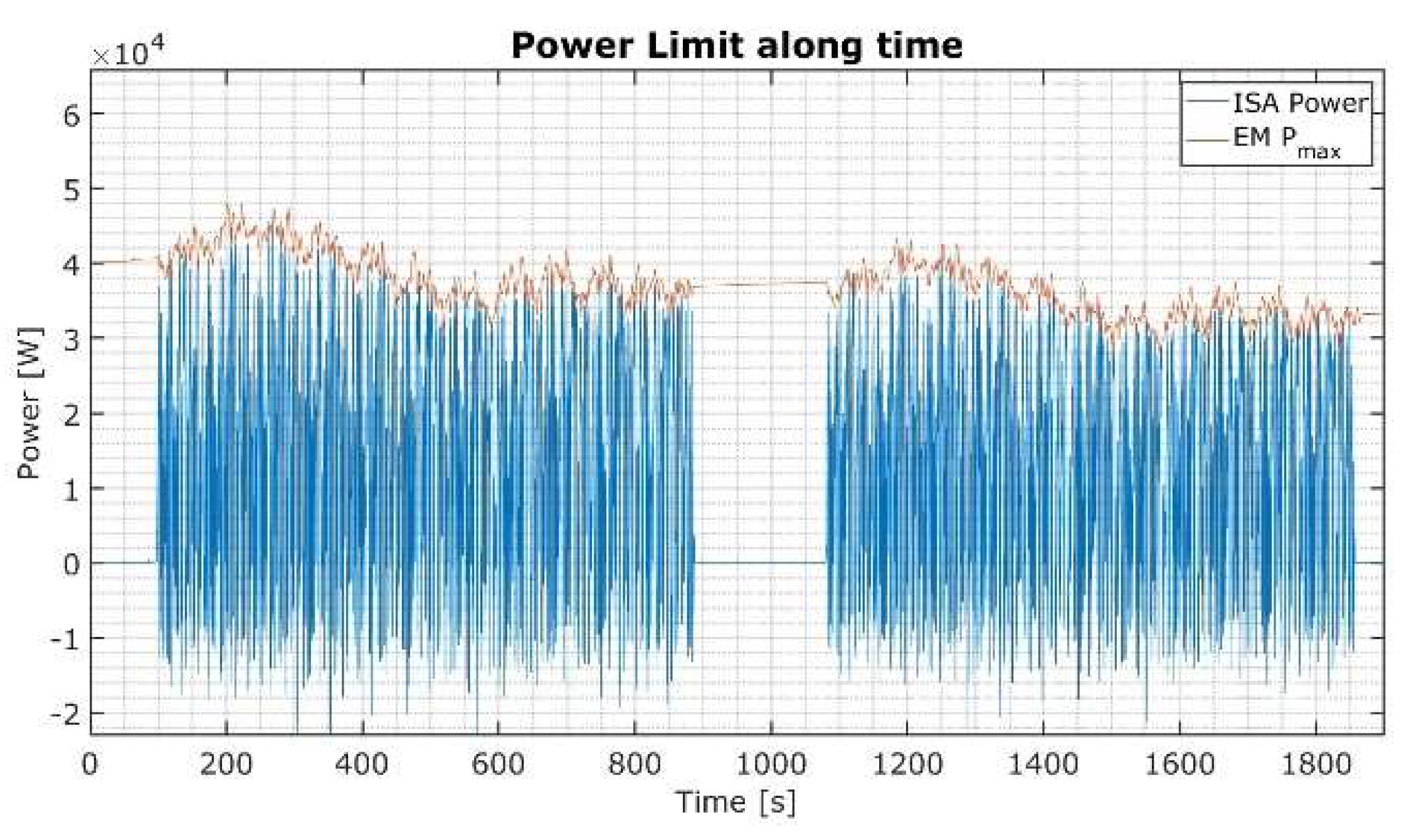
Table 7, with each respective deviation. Furthermore, the power limit adjustments over time compared to the real power output are shown in
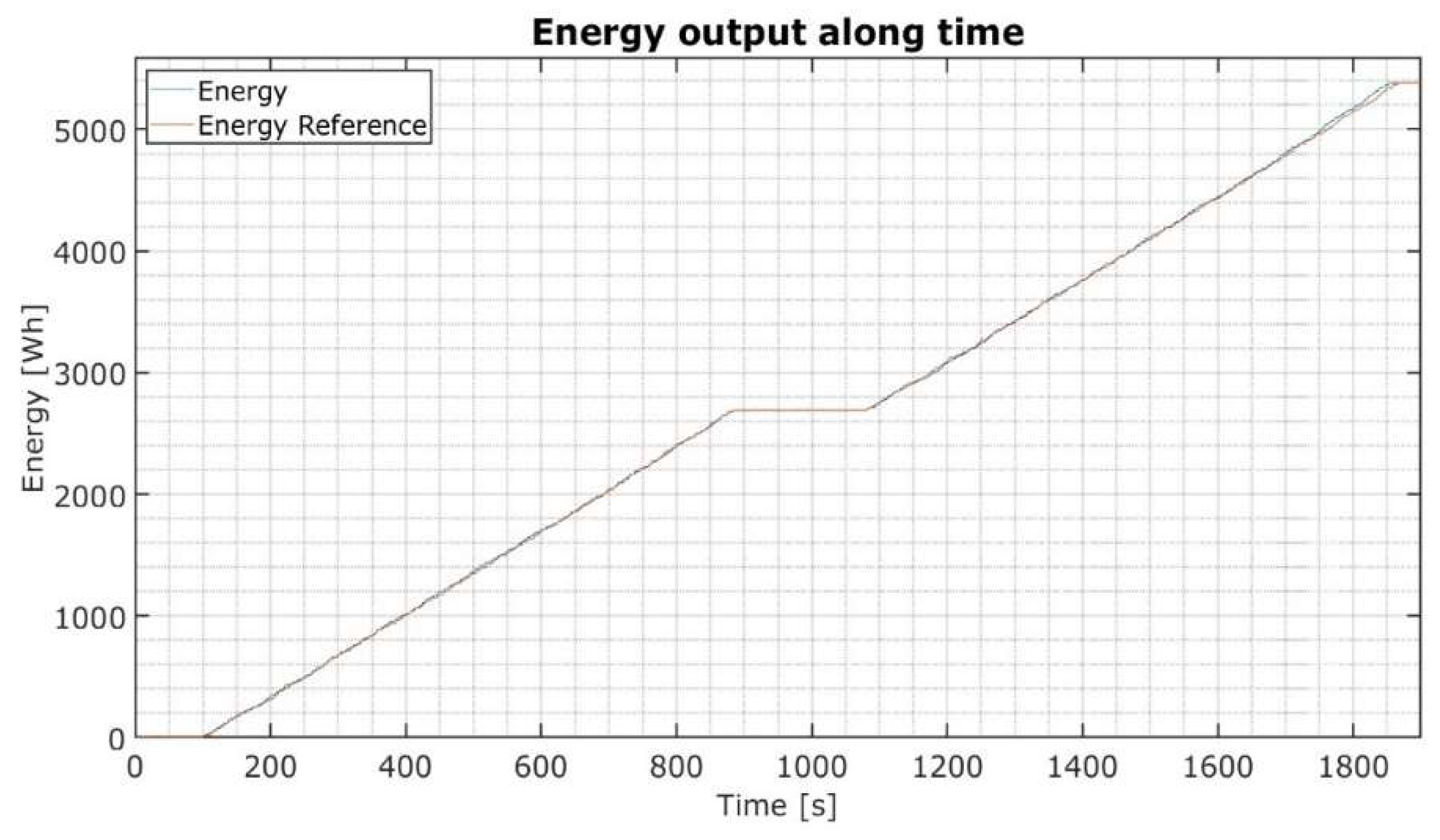
Figure 16, and one can see that over the run, it allows for proper adherence to the energy reference line, as shown in
Figure 17. The run’s total distance estimation resulted in 19894m, which deviates from the expected measured 19448m (22 laps of 884m each) by 2%.
It is important to acknowledge that while the achievements of a well-optimized offline simulation provide a strong foundation, they may not entirely capture the complexities of an actual Endurance event. In the dynamic context of an Endurance event with multiple participating cars, various factors come into play that can significantly impact the optimization process. These include unforeseen events such as yellow flags resulting from vehicle breakdowns or blue flags to inform slower-moving cars that they must temporarily pull over to a designated area to allow a faster car to overtake, both of which request unaccounted-for driver responses. Such occurrences disrupt the anticipated optimization outcomes.
Additionally, the driver change halfway through the Endurance event introduces additional challenges. Penalties are not accounted for in the optimization yet occur occasionally and have the potential to push the vehicle beyond the boundaries of the efficiency scoring window. Consequently, there may come a point where prioritizing pure speed over efficiency becomes more advantageous for the point-scoring tally.
These aspects highlight the need for future research to delve deeper into the intricacies of real-world scenarios and refine optimization strategies to adapt to the event-evolving dynamics of Formula Student Endurance events.
4. Conclusions
This work proposes a methodology to optimize the energy use of competitive electric vehicles and implement it in a real case study. The Formula Student competition was used as an implementation case to evaluate this methodology.
The methodology first requires complete vehicle characterization, involving the development of models grounded in the principles of vehicle dynamics. These models were validated, utilizing a data-driven approach to define powertrain efficiency and the battery pack’s capacity. The employed vehicle model provides a mismatch to reality under 5% for both velocity and energy model outputs during a full racing lap around the FSG track.
An optimization-based simulation framework was established to simulate Endurance runs, with the flexibility to configure key parameters such as powertrain characteristics and the starting conditions of the run. The overall goal is to maximize the points scored according to the regulations based on the driving profile and subsequent optimal energy deployment over distance. Following this, we developed an energy management system capable of employing a low-level controller that periodically dynamically adjusts the prototype’s maximum power limitation along the run. This involved continuously monitoring the real-time error, calculated as the difference between the reference and actual energy consumed, as measured by an appropriate sensor.
The proposed methodology was validated in a real Endurance run at a test track. The developed energy management control system was implemented, guided by a previously simulated optimal reference. This reference was tailored to maximize Endurance and Efficiency points in the new track layout relative to a normalized best score. In summary, compared to the optimal simulation, a 20km Endurance run had a total time mismatch of 1.4% and a total energy mismatch of 0.5%, leading to a discrepancy of 6.8% from the simulated and actual points prospect.
This approach, merging theoretical modeling with a data-driven perspective and testing the prototype, proved to be an efficient energy optimization method for electric vehicle applications, particularly the Formula Student Endurance competitions.
Author Contributions
Conceptualization, methodology, T.R.P. and J.F.P.F.; validation, T.R.P., J.F.P.F. and P.J.C.B.; formal analysis, investigation, T.R.P.; resources, T.R.P. and J.F.P.F.; writing—original draft preparation, writing—review and editing, T.R.P., J.F.P.F. and P.J.C.B.; supervision, J.F.P.F. and P.J.C.B. All authors have read and agreed to the published version of the manuscript.
Funding
This work is financed by national funds through FCT - Foundation for Science and Technology, I.P., through IDMEC, under LAETA, project UIDB/50022/2020.
Conflicts of Interest
The authors declare no conflict of interest.
References
- Wu, Q.; Sun, S. Energy and Environmental Impact of the Promotion of Battery Electric Vehicles in the Context of Banning Gasoline Vehicle Sales. Energies 2022, 15, 8388. [Google Scholar] [CrossRef]
- H. Borhan, A. H. Borhan, A. Vahidi, A. Phillips, M. Kuang, I. Kolmanovsky, and S. Cairano. Mpc-based energy management of a power-split hybrid electric vehicle. IEEE Transactions on Control Systems Technology 2012. [Google Scholar]
- Bauman, J.; Kazerani, M. A Comparative Study of Fuel-Cell-Battery, Fuel-Cell-Ultracapacitor, and Fuel-Cell-Battery-Ultracapacitor Vehicles. IEEE Trans. Veh. Technol. 2008, 57, 760–769. [Google Scholar] [CrossRef]
- Khaligh, A.; Li, Z. Battery, Ultracapacitor, Fuel Cell, and Hybrid Energy Storage Systems for Electric, Hybrid Electric, Fuel Cell, and Plug-in Hybrid Electric Vehicles: State of the Art. IEEE Trans. Veh. Technol. 2010, 59, 2806–2814. [Google Scholar] [CrossRef]
- B. Bilgin and A. Emadi. Electric Motors in Electrified Transportation: A step toward achieving a sustainable and highly efficient transportation system. IEEE Power Electronics Magazine 2014, 1, 10–17. [Google Scholar] [CrossRef]
- Massimiliano Gobbi, Aqeab Sattar, Roberto Palazzetti, Gianpiero Mastinu, Traction motors for electric vehicles: Maximization of mechanical efficiency – A review. Applied Energy 2024, 357.
- Cabuk, A.S.; Ustun, O. In Search of the Proper Dimensions of the Optimum In-Wheel Permanent Magnet Synchronous Motor Design. Energies 2024, 17, 1106. [Google Scholar] [CrossRef]
- Lin, W.; Zhao, H.; Zhang, B.; Wang, Y.; Xiao, Y.; Xu, K.; Zhao, R. Predictive Energy Management Strategy for Range-Extended Electric Vehicles Based on ITS Information and Start–Stop Optimization with Vehicle Velocity Forecast. Energies 2022, 15, 7774. [Google Scholar] [CrossRef]
- J. F. P. Fernandes et al., Extended-Range Marine Unmanned Surface Vehicles for Border Surveillance Missions, 2024 IEEE 22nd Mediterranean Electrotechnical Conference (MELECON), Porto, Portugal, pp. 960–965, 2024.
- X. Liu, A. X. Liu, A. Fotouhi, and D. Auger. Optimal energy management for formula-e cars with regulatory limits and thermal constraints. Applied Energy 2020. [Google Scholar]
- F. S. Germany. Formula student rules 2023, 2023. [Online]. Available online: https://www.formulastudent.de/fileadmin/user_upload/all/2023/rules/FS-Rules_2023_v1.0.
- Formula Student, FST Lisboa official website. Available online: https://www.fstlisboa.com/.
- F. S. Germany. Formula Student Germany competition results. Available online: https://www.formulastudent.de/fsg/results.
- AMK, Amk motion - electric racing kit. 2520. Available online: https://www.amk-motion.com/amk-dokucd/dokucd/en/DokuCD_HTML5_en.htm#projekt/doku-cd_html5/topics/amk_automotive.htm?
- W. Milliken and D. Milliken. Race Car Vehicle Dynamics, 1995.
- H. Pacejka. Tyre and Vehicle Dynamics, 2006.
- Jia, Y.; Jibrin, R.; Görges, D. Energy-Optimal Adaptive Cruise Control for Electric Vehicles Based on Linear and Nonlinear Model Predictive Control. IEEE Transactions on Vehicular Technology 2020, 69, 14173–14187. [Google Scholar] [CrossRef]
- J. C. Leger. Menger curvature and rectifiability. Annals of Mathematics 1999.
- S. Tie and C. Tan. A review of energy sources and energy management system in electric vehicles. Renewable and Sustainable Energy Reviews 2013.
Figure 1.
Methodology flowchart.
Figure 1.
Methodology flowchart.
Figure 2.
The FST12 prototype, used as our case study, was the platform for testing the real-time implementation.
Figure 2.
The FST12 prototype, used as our case study, was the platform for testing the real-time implementation.
Figure 3.
Rear motor eff. map with Pmax = 40kW and =21 Nm.
Figure 3.
Rear motor eff. map with Pmax = 40kW and =21 Nm.
Figure 4.
Bicycle model geometry and parameters.
Figure 4.
Bicycle model geometry and parameters.
Figure 5.
Endurance Event - Track layout.
Figure 5.
Endurance Event - Track layout.
Figure 6.
Velocity limit along FSG23 track layout.
Figure 6.
Velocity limit along FSG23 track layout.
Figure 7.
Developed a simulator for energy optimization.
Figure 7.
Developed a simulator for energy optimization.
Figure 8.
FSG23 Endurance offline distance estimation.
Figure 8.
FSG23 Endurance offline distance estimation.
Figure 10.
Velocity mismatch factor along lap.
Figure 10.
Velocity mismatch factor along lap.
Figure 11.
Velocity along FSG lap time.
Figure 11.
Velocity along FSG lap time.
Figure 12.
Optimized power deployment along FSG track.
Figure 12.
Optimized power deployment along FSG track.
Figure 13.
Optimized FSG scoring result in joint score map.
Figure 13.
Optimized FSG scoring result in joint score map.
Figure 14.
Optimized lap velocity profile along Alverca track.
Figure 14.
Optimized lap velocity profile along Alverca track.
Figure 16.
Vehicle power output and limitation along time.
Figure 16.
Vehicle power output and limitation along time.
Figure 17.
Energy consumption in comparison to its reference along time.
Figure 17.
Energy consumption in comparison to its reference along time.
Table 1.
Deduction of total available battery pack capacity.
Table 1.
Deduction of total available battery pack capacity.
| Theoretical capacity |
7666 Wh |
|
35 mins) |
350 Wh |
| Battery pack losses (3%) |
230 Wh |
| Deviation losses (10%) |
767 Wh |
| Available capacity |
6319 Wh |
Table 2.
Maximum capacity extrapolation from Endurance data.
Table 2.
Maximum capacity extrapolation from Endurance data.
| Endurance Results |
FSG23 |
FSS23 |
| Initial SOC |
98.6 % |
98.99 % |
| Final SOC |
15.2 % |
17.73 % |
| Energy consumption |
5.324 kWh |
5.139 kWh |
| Available capacity |
6.405 kWh |
6.324 kWh |
Table 3.
Resulting formula values from FSG 2023.
Table 3.
Resulting formula values from FSG 2023.
| FSG2023 |
Value |
| Tmax |
1396.84 = 1862 s |
| EFmin |
s2
|
| EFmax |
s2
|
Table 4.
Different odometry methodologies results.
Table 4.
Different odometry methodologies results.
| Log Run |
Inertial odom. |
Actual distance |
| Alverca |
21250 m |
21378 m |
| FSG23 |
22070 m |
21924 m |
| FSS23 |
20760 m |
20900 m |
Table 5.
Velocity and energy mean-squared error model mismatch.
Table 5.
Velocity and energy mean-squared error model mismatch.
| Mean-squared-error |
Velocity [m/s] |
Energy [Wh] |
| Point mass vehicle model |
2.96 |
33.92 |
| Dynamic bicycle model |
0.48 |
2.26 |
Table 6.
Velocity and energy mean-squared error simulation mismatch.
Table 6.
Velocity and energy mean-squared error simulation mismatch.
| Mean-squared-error |
Velocity [m/s] |
Energy [Wh] |
| Continuous lap simulation |
0.48 |
2.26 |
| Discretized lap simulation |
0.57 |
3.47 |
Table 7.
Final run results in comparison to the optimization.
Table 7.
Final run results in comparison to the optimization.
| Results |
Time [s] |
Energy [kWh] |
Points |
| Optimization |
1522.1 |
5.355 |
271.8 |
| Final run |
1574.6 |
5.383 |
253.1 |
| Deviation |
1.4% |
0.5% |
6.8% |
|
Disclaimer/Publisher’s Note: The statements, opinions and data contained in all publications are solely those of the individual author(s) and contributor(s) and not of MDPI and/or the editor(s). MDPI and/or the editor(s) disclaim responsibility for any injury to people or property resulting from any ideas, methods, instructions or products referred to in the content. |
© 2024 by the authors. Licensee MDPI, Basel, Switzerland. This article is an open access article distributed under the terms and conditions of the Creative Commons Attribution (CC BY) license (http://creativecommons.org/licenses/by/4.0/).