Submitted:
31 October 2024
Posted:
01 November 2024
You are already at the latest version
Abstract
This paper aims to present a particular study of the performances of electric vehicles based on real driving conditions on a cycle carried out using the general conditions of Regulation (EU) 1832/2018 regarding RDE tests. In this sense, a modern electric SUV was used and the experimental tests were made using a measuring equipment connected to the vehicle via the OBD2 plug. In the following, the experimental results will be analyzed and presented and the main influencing factors on the energy performance that may occur in real running conditions will be identified.
Keywords:
Electric SUV
; State of Charge
; Energy Consumption
1. Introduction
In order to study the behavior of an electric vehicle and to take into account all the existing influencing factors, this paper approaches the determination of the performances in real driving conditions for an electric vehicle, with the aim of identifying all the advantages as well as the disadvantages of using an electric vehicle in different driving areas (e.g. urban, extra-urban or motorway). Purpose of the experiment is the detailed analysis of the variation of energy consumption on a predetermined route and the variation of autonomy, taking into account internal and external factors that influence these performances and the subsequent analysis of sustainable solutions to optimize dynamic and energetic performances of an electric vehicle, [1].
Although the determination of pollutant emissions is not aimed at as there is no logical basis for this for an electric propulsion system, some hardware and software equipment is still needed to facilitate communication with the vehicle and allow the recording of some data of interest that can later be used in the validation of the realized simulation model, such as for example the speed profile of the real cycle, the obtained energy consumption and the autonomy of the vehicle.
In order to achieve all these points and to comply with some basic conditions regarding the measurement on a real cycle, the existing conditions in the European regulations (EU) 2017/1151 and (EU) 2018/1832 with their amendments will be analyzed and used. The basic conditions also apply to an electric vehicle when determining its energy consumption and range.
Also, the paper proposes a comparative analysis using the numerical simulation of the dynamic and energetic performances of an electric SUV vehicle when running on a real cycle and on a standardized cycle (WLTC - Worldwide Harmonized Light Vehicles Test Cycle). Through the multitude of results obtained from the simulation and through the optimization of the basic model in accordance with certain internal and external factors of influence, a tool for experimental research of the performance of electric vehicles is developed that can be used by specialists in the field of scientific and research activity, as well as in the elaboration of future studies with a role of optimization or development, conclusive for this branch of the industry.
In the following sections, there will be analyzed in turn: the structure of the vehicle used for the experimental research, the conditions that were taken into account in accordance with the mentioned regulations and the experimental results obtained.
2. Materials and Methods
2.1. Electric Vehicle Specifications
The Skoda ENIAQ iV 80 model, which is the first electric SUV produced by Skoda, was chosen for the experimental test taking into account the requirements for running in all areas mentioned in the regulation (EU) 2018/1832. The constructive particularity of this vehicle is related to the platform on which the propulsion system is mounted called MEB (Modularer E-Antriebs-Bauksten) [2], in translation a modular kit that allows the implementation of an electric propulsion system. This platform is common in the VAG group and has the advantage that it can be used on several models of electric vehicles. In experimental research, the model used is the one organized according to the "everything behind" solution.
2.2. Legislative Conditions Imposed for Experimental Research
ANNEX III A from [3] presents several types of requirements and conditions that must be taken into account when carrying out RDE homologation tests. Given that this work strictly addresses a vehicle equipped with an electric propulsion system, only a part of the respective conditions that apply regardless of the type of fuel or propulsion system used were extracted for the experiments.
These conditions were tracked and taken into account in the experimental measurements in this paper as follows:
- Driving in an urban environment is characterized by speeds lower than or equal to 60 km/h;
- Rural driving is characterized by speeds greater than 60 km/h and less than or equal to 90 km/h;
- Driving on the highway is characterized by speeds over 90 km/h;
- The cycle must consist of approximately 34% urban driving, 33% rural driving and 33% highway driving;
- The duration of the cycle must be between 90 and 120 minutes;
- The minimum distance for each type of driving (urban, rural and highway) must be 16 km.
2.3. The Equipment Used to Carry Out the Experimental Tests
Considering the fact that the experimental tests are based on running on a real cycle in order to be able to make the necessary data acquisition, the Bosch KTS 590 module from ESI [tronic] is used. This device allows a quick and efficient connection between the vehicle and a laptop by means of a cable that connects through the OBD socket and allows communication with the vehicle's computer. KTS is part of the category of multi-brand devices with the possibility of connecting to most vehicles on the market and is a module that deals with the diagnosis of control units. The advantage of using the KTS module in the experimental tests in this paper is related to the fact that it can be supplied with voltage directly through the OBD plug, which allows driving for a longer period of time with the vehicle without the need for an external energy source which also simplified the location of the data acquisition "installation" in the vehicle.
Using the connection with the vehicle's computer through the OBD socket and the communication with the CAN network, the KTS module allows the measurement of several characteristic quantities in real time, on the set driving cycle, and in addition to this, it also allows saving the graphs obtained as a function of time and later conversion of files in the form of which they are automatically saved in the device's memory, into .xlsx type files that allow fast processing of the measured data and help in the detailed analysis of the obtained experimental results. Figure 1 shows a schematic diagram of how to connect the KTS module to the vehicle's OBD socket alongside the laptop used as an interface for module command and control and data acquisition:
The following parameters were extracted through the KTS module:
- Variation of speed over time;
- The variation of the speed of the electric motor over time;
- Electric motor torque – driver option;
- Battery state of charge (SOC) over time;
- Variation of the working voltage of the traction battery;
- The variation in the intensity of the electric current absorbed by the inverter from the traction battery;
- Energy consumed on the actual cycle performed – [kWh];
- Energy consumption on the real cycle achieved – [kWh/100 km].
2.4. Route Selection and Vehicle Instrumentation
The tests were carried out in Bucharest and outside, in its vicinity and the starting point was in the inner yard of the Faculty of Transport, in the laboratory area of the Department of Road Vehicles where the vehicle was charged at 11 kW/32A station and where its instrumentation was carried out. Then, in order to avoid changing the slope of the road, the direct exit through „Iuliu Maniu” Boulevard was avoided and the area from „Doina Cornea” Boulevard was chosen, after which the route followed its course to „Virtutii” Road through „Iuliu Maniu” Boulevard, then on „Splaiul Independetei” to Northern Railway Station and finally on „Calea Grivitei” towards the exit from Bucharest towards Chitila. This portion constituted the running part in the urban area, until the exit on the Bucharest Ring Road. Then, the route continued on the belt until the entrance to the A3 Bucharest-Ploiesti Highway, a portion considered the extra-urban cycle, and finally a part of the Highway was traveled to complete the cycle. Obviously, through the higher speeds required to achieve the extra-urban cycle and the one on the highway, they determined the increase in the distance traveled so that the time is proportional to that in the urban environment.
The route is presented in Figure 2 through points of interest that helped shape it:
Instrumentation of the vehicle consisted of connecting the KTS module to the OBD plug of the vehicle located in the driver's seat area, on the left side under the steering wheel, and making the connection between the module and the laptop with the KTS ESI [tronic] interface where the parameters were monitored and stored track throughout the trials. In order to ensure the best possible contact during the tests and to avoid disconnection of the diagnostic module in the event of vibrations or involuntary touches by the pilot, the cable was fixed to certain points in the steering wheel area, and the connection plug was secured by adhesive tape and plastic tie bands. Figure 3 shows the equipment and instrumentation of the vehicle made before the start of the tests:
2.5. Hipothesese Established for Carrying out the Experiments
To carry out the tests, Friday was chosen, the time interval 12-15 pm. In accordance with the conditions in Section 2.2, a series of basic assumptions were established for modelling the route and making a cycle as conclusive as possible for the analysis and study of the dynamic and energetic performances of the electric vehicle used for the tests. These assumptions are based both on the conditions in the regulation and on the dynamic performances of the vehicle and external factors that may influence the tests.
Thus, the assumptions are the following, [1]:
- The vehicle was driven on level road sections where the angle of inclination was 0°;
- The altitude of the entire route was considered constant at around 75 m (the altitude of the city of Bucharest);
- The average temperature in the predetermined time interval was around 10°C;
- The wind speed was low enough to not significantly influence the aerodynamic resistance of the electric vehicle;
- The quality of the track was very good throughout the route, without bumps, obstacles or other factors that could influence the experimental measurements;
- All sections of the road were dry and passable under normal speed conditions according to the limits established by law;
- In all three areas of the completed cycle, the driving speed was adapted to the limits in force according to the law and there were no exceeding of these limits;
- Traffic lights were taken into account, without forcing the passage, pedestrian crossings, roundabouts and unforeseen traffic situations where it was necessary to reduce speed;
- The battery state of charge at the start of the route was 100%. A longer time has been considered for the charging process to allow the battery cells to stabilize and not be additionally and unnecessarily stressed;
- The total mass of the vehicle consisted of the own mass of the electric vehicle, the mass of the pilot and the companion and the mass of the measuring equipment – 2325 kg;
- The air pressure in the tires was checked to ensure there were no differences or air losses.
3. Development of the Simulation Model
3.1. Simulation Environment
The study of systems using modeling and simulation has transformed the way scientists and engineers work by transferring to the computer many of the processes and tasks performed in the laboratory or in real running conditions. Currently, modeling and simulation are widely used for the synthesis of systems and their analysis, as well as for the development and verification of control algorithms [5].
Simulink is a dynamic systems modeling, simulation, and analysis environment that is a standard in academia and industry. It is included as a toolbox in the MATLAB environment, and this facilitates the interaction between the two environments allowing, among others, the rapid introduction of parameters, automation of simulations, processing and visualization of results [5].
In this study the implementation of the components of the electric propulsion system consisted in the creation of subsystems based on the principle of operation of each individual component along with the necessary mathematical equations that will be introduced in the simulation environment. The considered components are: the electric motor, vehicle transmission represented by a single-stage gearbox and the traction battery for which an existing block was used in the Simscape library from Simulink that allows the selection of the type of battery used and its parameterization according to the data provided by the manufacturer of the vehicle used.
The basic subsystems are:
- Electric SUV which contains part of the components of the electric propulsion system: the electric motor, the reducer, together with the „driver” subsystem and the system of equations represented by the resisting forces from which the general equation of rectilinear movement results. This subsystem connects to the real cycle used for simulation represented by the vehicle speed variation in time;
- Battery which has as input parameter Pbat which represents the total power absorbed from the battery during the cycle. For this subsystem an existing block in the Simscape library („Driveline” – „Power Sources”) from Simulink was used which allows the parameterization of the battery according to the characteristics of the studied vehicle;
- Power and Energy Calculation was added to the model to calculate Pbat. Mm (motor torque, [Nm]) and nm (motor speed, [rpm]) are defined as the input parameters of this subsystem. Outputs of this subsystem represent the basic electrical quantities for energy performance analysis: Pbat [kW] and Energy [kWh];
- Measurements is a subsystem created to process the results obtained through simulation and to determine other quantities of interest ( consumption [kWh/100 km] and autonomy [km] ) based on mathematical equations defined in [6];
The simulation model for the electric vehicle can be seen in the Figure 4:
To determine the autonomy a condition was implemented whereby the model operates until the battery discharges to the value at which recharging becomes necessary. As a rule the BMS (Battery Management System) system allows the operation of the traction battery up to a state of charge of 20% and in general this value is specific to lithium batteries because if it is discharged below 20%, the charging process becomes complicated, there is a risk of cell imbalances which can cause their irreparable damage, [7,8]. The imposed condition consisted of the „State Of Charge” signal connected to a „Compare to Constant” operator and a „Stop Simulation” block. In this way the comparison operator checks in real time during the simulation the values of the state of charge and when it reaches the value of 20%, the „Stop Simulation” block comes into operation which stops the simulation.
For real driving cycle a „Signal Builder” block was used which has no limitations related to the number of entered values and allows the signal to be imported as an „.xlsx” file where the data must be placed in consecutive columns and each sheet must be private and contains a single quantity as a function of time.
3.2. Conditions for Simulation
To carry out the simulations, several characteristic data of the used vehicle were used in accordance with the information provided by the manufacturer. These data will be presented in tables as follows: ,
Along with these parameters, a series of simplifying conditions presented in Table 4 were introduced in the simulation model:
3.2. Standardized Cycle – WLTC
WLTC is more advantageous than other standardized cycles (e.g.: NEDC) in terms of driving style being characterized by strong and frequent accelerations, followed by short braking, which causes the new procedure to be much closer to real driving conditions. Table 5 shows the main characteristics of the cycle:
WLTC consists of four phases: Low, Medium, High, Extra High. In the case of the procedure, there is also a classification of vehicles according to the class they belong to, the classification criterion being the specific power (Pspecific [W/kg]): Class 1, Class 2 and Class 3 [10].
The electric SUV used for the simulation is characterized by a specific power of ~ 72.3 W/kg so it falls into Class 3, and from the point of view of velocity in Class 3b with a maximum value of 160 km/h.
The WLTC cycle is represented in Figure 5:
4. Results
In this section, the results of the study will be presented one by one, starting with the experimental measurements made using the specialized equipment, and these results will be used for the validation of the simulation model and then for the performance study on the WLTC cycle.
4.1. Experimental Results
According to the experimental measurements, the real cycle completed had a duration of 5676 seconds, so approximately 95 minutes, and the total traveled distance on the established route was 77 km. The average speed in the urban environment was 19.7 km/h, and the maximum speed reached on the highway was 131 km/h in accordance with the legislation in force. By complying with all the traffic rules and adapting the driving speed according to the traffic conditions the following real driving cycle based on the conditions specified in the regulation (EU) 1832/2018, Annex III, presented in Figure 6 was obtained:
The distance covered on the established route was 77 km and the maximum acceleration reached was 2.81 m/s2 while the maximum deceleration was ~8.32 m/s2. Figure 7 show the variation of the acceleration during the cycle:
Other parameters measured and processed were: the state of charge of the battery (Figure 8), the total energy absorbed from the battery (Figure 9) and the energy consumption (Figure 10):
The total energy absorbed from the battery during the driving cycle was another parameter measured and recorded and its variation is represented in Figure 9.
After completing the route and completing the cycle of measurement the value of 16.77 kWh was obtained energy consumed for traveling 77 km. Based on the variation of total energy during the cycle, Figure 10 shows the variation of energy consumption during the proposed cycle:
The variation of energy consumption on the established route was also recorded and the value obtained it was 21.78 kWh/100 km (Figure 10). In [11] where the consumption values are presented depending on the driving regime and the area, an average of energy consumption between driving in the city (urban environment), extra-urban and highway is presented by the manufacturer. To compare this value with the measured one the results are centralized in Table 6:
Regarding the autonomy of the vehicle obtained when running on the real cycle proposed in this work it was considered to cover the route until the state of charge of the traction battery reaches the value of 20%, at which point a distance of 373.3 km was determined, which represents the value of the autonomy when running on a real cycle.
In [11] a series of autonomy values for the three phases or driving environments is presented, respectively a global value combined over a cycle formed by all three phases similar to the one proposed in the paper. Thus, for the urban environment the autonomy is 365...400 km, for the extra-urban environment 300...330 km, and for the highway 205...225 km, resulting in a global combined value of the three phases of 337 km. Table 7 shows a comparison between the autonomy proposed by the manufacturer and the measured one.
4.2. Simulation Results
This section proposes a comparative analysis between the experimental results obtained by measurements in real running conditions on the proposed cycle and the results of simulations using the presented model. This comparative analysis is substantiated by the need to validate the model developed for the study of the performances of electric vehicles and to identify the similarities or major inadvertences between the real, measured and simulated values in order to search for optimization solutions of the model to simulate as well as possible and to follow, with as few errors as possible a run cycle. For these reasons, in the following, a series of diagrams will be presented that represent the overlap of the variation of the measured quantities with those resulting from the simulations, and the values of interest for certain quantities will be compared, and relative errors will be calculated based on them.
However, it should be noted that although the simulation model has been implemented as many functions as possible to follow real driving conditions in terms of road quality, unforeseen traffic situations, weather conditions, ambient temperature, as well as basic characteristics constructive and dynamic of the vehicle used for the experimental measurements, the existence of some errors between the real and simulated values is natural since the model cannot provide the results with 100% efficiency. The errors resulting from the comparison of the two situations are necessary for further optimizations and will support the model in becoming a tool for analyzing the performance of electric vehicles.
4.2.1. Real Cycle
The main quantity of interest is the speed of the vehicle along the proposed cycle. Figure 11 graphically shows the comparison between the two profiles, the real (measured) and the simulated:
A deviation of the speed profile in relation to the reference one with a margin of ±2 km/h is admitted and accepted [3]. In this sense, the verification of this deviation in several points of the diagram from Figure 11 was followed and an area was identified where the maximum deviation was + 0.15 km/h, and the minimum was - 0.2 km/h, values that respect the interval in the regulation. Figure 12 shows the detail regarding the deviation of the two speed profiles:
The comparative studies for the state of charge of the battery and for the variation of the energy consumed during the cycle are presented in Figure 13 and Figure 14:
Regarding the state of charge of the battery, the final values obtained by both measurement and simulation are extremely close: 83.5% - real (measured) and 82.31% - from simulation. From the point of view of the energy consumed during the driving cycle, the measured value according to the time variation was 16.77 kWh, while the simulation resulted in 15.99 kWh, so a difference of 0.78 kWh between the case real and simulation resulting in an error of 4.65%.
A comparison was also made between the measured consumption and the one resulting from the simulation, from which the following values were obtained: 21.78 kWh/100km - real (measured) and 20.76 kWh/100km - from the simulation, a situation in which it resulted an error of 4.68%. The comparative variation of energy consumption is shown in Figure 15:
4.2.2. WLTC
At first the deviation of the simulated profile in relation to the reference one (WLTC profile) was followed and for this the two profiles were overlapped as shown in Figure 16.
Regarding the acceleration profile in relation to the specialized literature [9] where the cycle characteristics are specified the simulation resulted in a maximum acceleration of 1.684 m/s2. The actual acceleration profile was obtained by time derivation the reference profile imported from Excel using the mathematical function ”Derivative" from Simscape library. The overlap of the two acceleration profiles is represented in Figure 17:
In terms of energy performances the WLTC cycle simulation resulted a battery SOC of ~95.95% with a 4.05% decrease from the initial value 100%. Variation of the SOC of the battery is represented in Figure 18.
Variation of the total energy absorbed during the cycle can be seen in Figure 19. The energy consumed on the WLTC cycle was 3.361 kWh a value that took into account the energy consumed by the auxiliary systems which, by analogy using the reference profile obtained through experimental measurements turned out to be 0.35 kWh.
The energy consumption obtained considering the distance covered during the cycle of ~23.3 km was 14.49 kWh/100 km (Figure 20).
To determine the autonomy on the WLTC cycle by simulation a time of 42000 s was set and the simulation was started. When the state of charge reached the value of 20%, the simulation stopped at tfinal = 40110 s and the distance of 512 km resulted, which represents the autonomy of the vehicle used for the research.
Next the results obtained from the simulation for the WLTC cycle are recorded and presented in Table 8 in order to be compared with values mentioned by the manufacturer through several specialized websites.
Table 9 compares the values obtained by simulation and those indicated by the manufacturer for tests on the WLTC cycle:
Taking into account Table 9 it can be seen that the relative errors are less than 5%.
5. Discussion
The state of charge of the battery at the start of the run cycle was 100%, after a controlled charging process and sufficient time for stabilization. On the urban driving phase SOC decreased by 3.5% so it reached 96.5%, after which on the extra-urban driving phase decreased by another 4.5%, thus meaning 92% and finally on the phase of running in regime of highway where speeds were higher state of charge dropped to 83.5% so by another 8.5% moment when the vehicle was stopped and the measurements completed. Thus, on the chosen route the state of charge decreased by a total of 16.5% (Figure 8).
The average value of the energy absorbed from the battery on each phase of the proposed cycle was determined, resulting in the following values: urban driving phase – 1.72 kWh; extra-urban driving phase – 3.22 kWh and highway phase – 12.4 kWh.
The proposed real cycle was used in a period with low temperatures, an aspect that constituted a negative influencing factor on energetic performances.
The speed profile obtained experimentally was influenced by the pilot's driving style and also by the portions chosen for the cycle but especially the speed limits in force according to Romanian law.
When driving at speeds below 60 km/h, with an average speed of 19.7 km/h and short and frequent braking due to the existence of traffic lights and busy intersections, the state of charge experienced slight increases generated by regenerative braking, which demonstrates from a practical point of view, the fact that an electric vehicle lends itself extremely well to driving in the urban environment.
In the extra-urban area, namely the ring road of the capital, the northern part where the speed limits allowed the realization of the second phase of the cycle where the driving speed could be maintained in the range of 60...90 km/ h, there were still sections where it was necessary to decelerate to very low speeds, or sometimes even to a stop where pedestrian crossings or roundabouts were encountered.
The simulations carried out using the standardized cycle (WLTC) aimed to analyze the operation mode of the simulation model proposed in this work and to diversify the research regarding the determination of the dynamic and energetic performances of an electric vehicle.
6. Conclusions
Through the comparative analysis between the results obtained experimentally and those from the simulation, errors between 0...5 % resulted, which gives the simulation model a high degree of confidence in its use for other more complex studies.
The differences between the values obtained experimentally and those from the simulation using the real speed profile are generated by the fact that certain conditions and situations encountered in reality cannot be 100% implemented in a mathematical simulation model such as the precision of the developed subsystems, certain settings in the program options regarding the chosen step, the type of solver, as well as certain conditions that cannot be physically modeled or simulated similar to the traffic reality.
The main objective of this study was to develop an original mathematical model using the modeling-simulation program MATLAB – Simulink that allows the analysis of the dynamic and energetic performances of an electric vehicle, especially from the M1 and N1 categories using a real driving cycle or a standardized one (in this paper: WLTC).
As a result of this research it was found that the operating mode of an electric vehicle considerably influences its real autonomy.
Through the multitude of results obtained using the simulation model in accordance with certain internal and external factors of influence a tool for researching the performances of electric vehicles has been developed that can be used by specialists in the field to develop and create future studies with the role of analysis and optimization of electric vehicles performances by implementing innovative solutions such as: multi-speed transmission, multiple electric motors.
Author Contributions
Carrying out experimental research and determining the real speed profile by measurement, A.A.A and C.A.R; simulation model development, A.A.A; simulation model optimization, A.A.A and C.A.R; processing of experimental data and results obtained from simulations, A.A.A; writing and organizing the paper, A.A.A, C.A.R, D.M.I; project administration, C.A.R and D.M.I. All authors have read and agreed to the published version of the manuscript.
Funding
This research was funded by National University of Science and Technology POLITEHNICA Bucharest, RO-060042, Romania by a grant from the National Program for Research of the National Association of Technical Universities - GNAC ARUT 2023.
Data Availability Statement
The original contributions presented in the study are included in the article; further inquiries can be directed to the corresponding author.
Acknowledgments
This work was supported by a grant from the National Program for Research of the National Association of Technical Universities - GNAC ARUT 2023.
Conflicts of Interest
The authors declare no conflicts of interest.
References
- Ancuța, A.A. , Research on the Determining the Dynamic and Energetic Performances of Electric Vehicles, Doctoral Thesis, National University of Science and Technology POILTEHNICA Bucharest, Faculty of Transport, June 2024. [Google Scholar]
- Individual study program - SSP (PDF) – Skoda ENIAQ, Service catalog, unpublished (made available to the authors by the Porsche Group Romania).
- Regulation (EU) 2018/1832 of the COMMISSION of 05.11.2018. Available online: https://eur-lex.europa.eu/legal-content/RO/TXT/HTML/?uri=CELEX%3A32018R1832#d1e39-105 -1 (accessed on 15.03.2024).
- Robert Bosch GmbH KTS, 560/590 (KTS 5a series) Module for control unit diagnosis, 1 689 989 223, 24.09.2021. Available online: http://mediathek.bosch-automotive.com/files/bosch_wa/989/223.pdf?_gl=1*q6h7u*_ga*NDY5MTIzNzgwLjE2OTY5NDUwMzk.*_ga_913VVKMZ46*MTcwNzIyNjUxMC40LjEuMTcwNzIyNjUyMS4wLjAuMA (accessed on 15.03.2024).
- Bățăuș, M. , Modern Automotive Transmissions: An Introduction in Modeling and Simulation, POLITEHNICA Press, Bucharest, 2018, ISBN 978-606-515-806-1.
- Ancuța, A.A. , Voloacă, Ș., Frățilă G., Danciu, Gr., Analysis of Energetic and Traction Performances for an Electric Vehicle in Real Driving Conditions, EAEC-ESFA Congress, National University of Science and Technology POILTEHNICA Bucharest, November 2023. Available in: IOP Conf. Ser.: Mater. Sci. Eng. 1303 012006, DOI 10.1088/1757-899X/1303/1/012006.
- Mehrdad, Ehsani; Yimin, Gao; Ali, Emadi; Modern Electric, Hybrid and Fuel Cell Vehicles – Fundaments, Theory and Design, Second Edition; Texas A&M University College Station, Texas, U.S.A.
- Larminie, J. Lowry, J. – Electric Vehicle Technology Explained – Oxford Brookes University, Oxford, U.K, ISBN 0-470-85163-5.
- ***https://en.wikipedia.org/wiki/Worldwide_Harmonised_Light_Vehicles_Test_Procedure (accessed on 27.03.2024).
- Regulation (EU) 2017/1151 of the COMMISSION of 01.06.2017. Available online: https://eur-lex.europa.eu/search.html?scope=EURLEX&text=2017%2F1151&lang=en&type=quick&qid=1709127536185 (accessed on 27.03.2024).
- ***https://www.automobile-catalog.com/auta_perf1.php#gsc.tab=0 (accessed on 28.03.2024).
- ***https://ev-database.org/car/1280/Skoda-Enyaq-iV-80 (accessed on 28.03.2024).
Figure 1.
Schematic diagram of the connection plan for KTS 560/590, [4]: 1 – OBD connection on board the vehicle; 2 – OBD connection cable; 3 – KTS module.
Figure 1.
Schematic diagram of the connection plan for KTS 560/590, [4]: 1 – OBD connection on board the vehicle; 2 – OBD connection cable; 3 – KTS module.
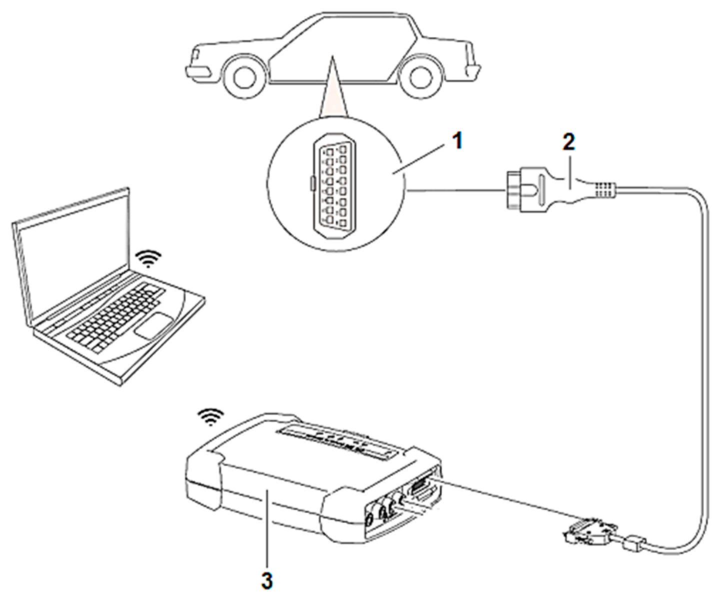
Figure 2.
Map of the route established for research.
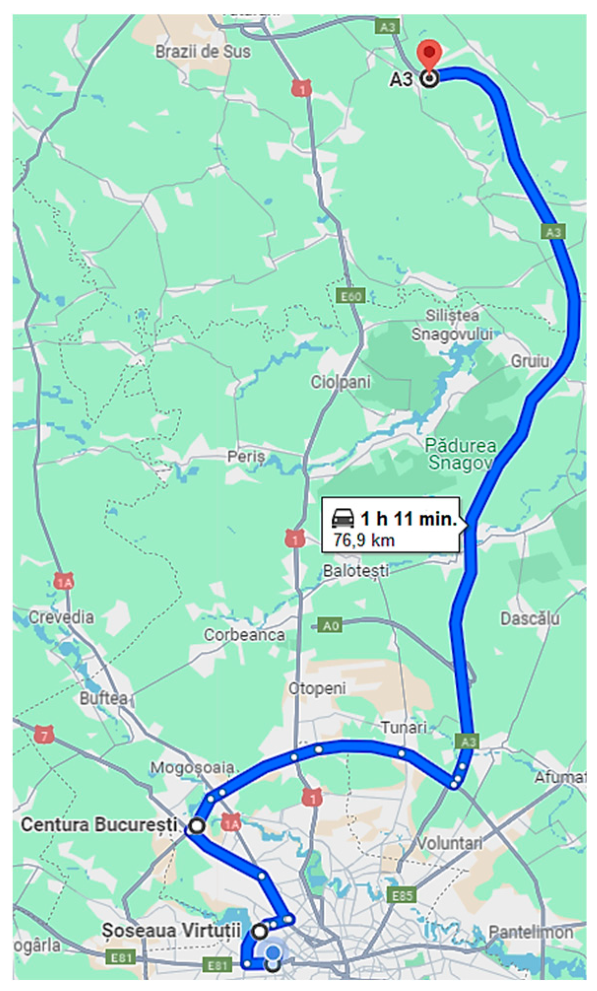
Figure 3.
(a) The KTS module and its connection with the OBD socket of the Skoda Eniaq vehicle; (b) sequence from experimental trails.
Figure 3.
(a) The KTS module and its connection with the OBD socket of the Skoda Eniaq vehicle; (b) sequence from experimental trails.
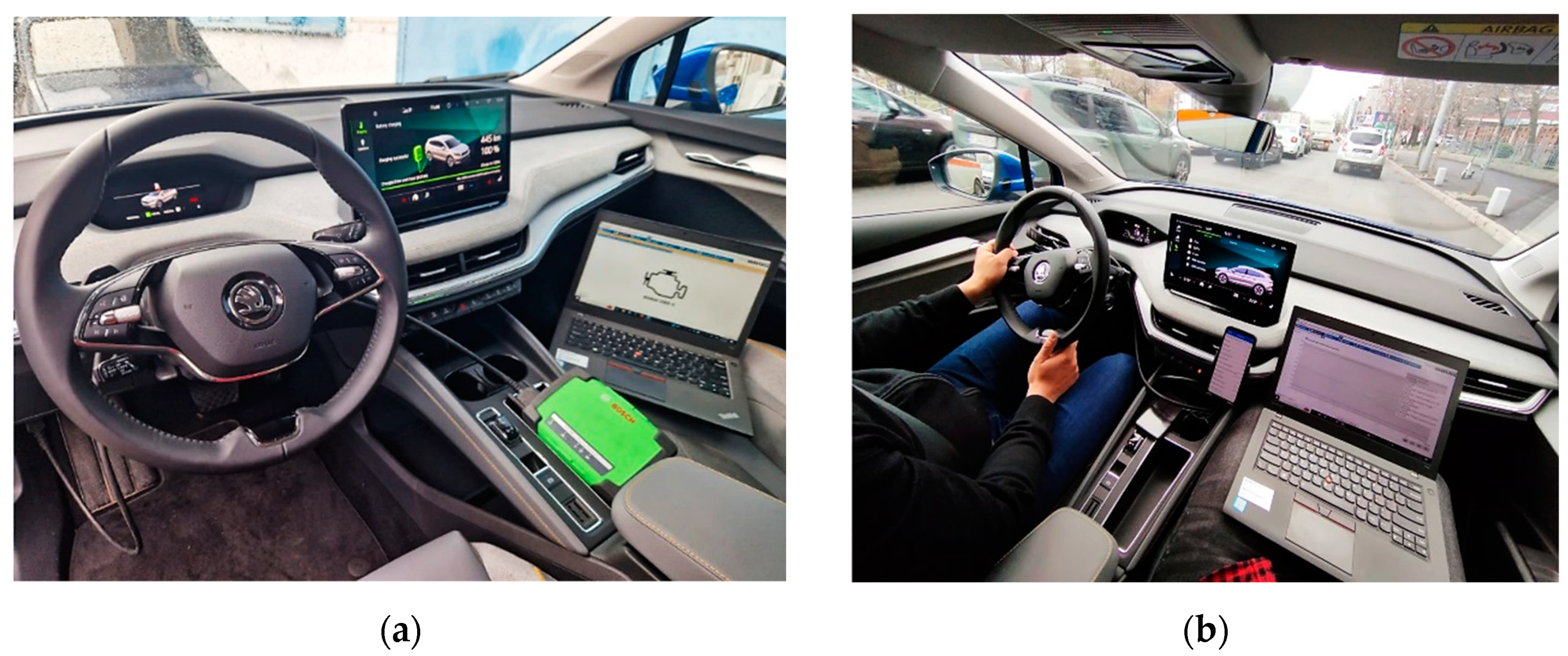
Figure 4.
Simulation model.
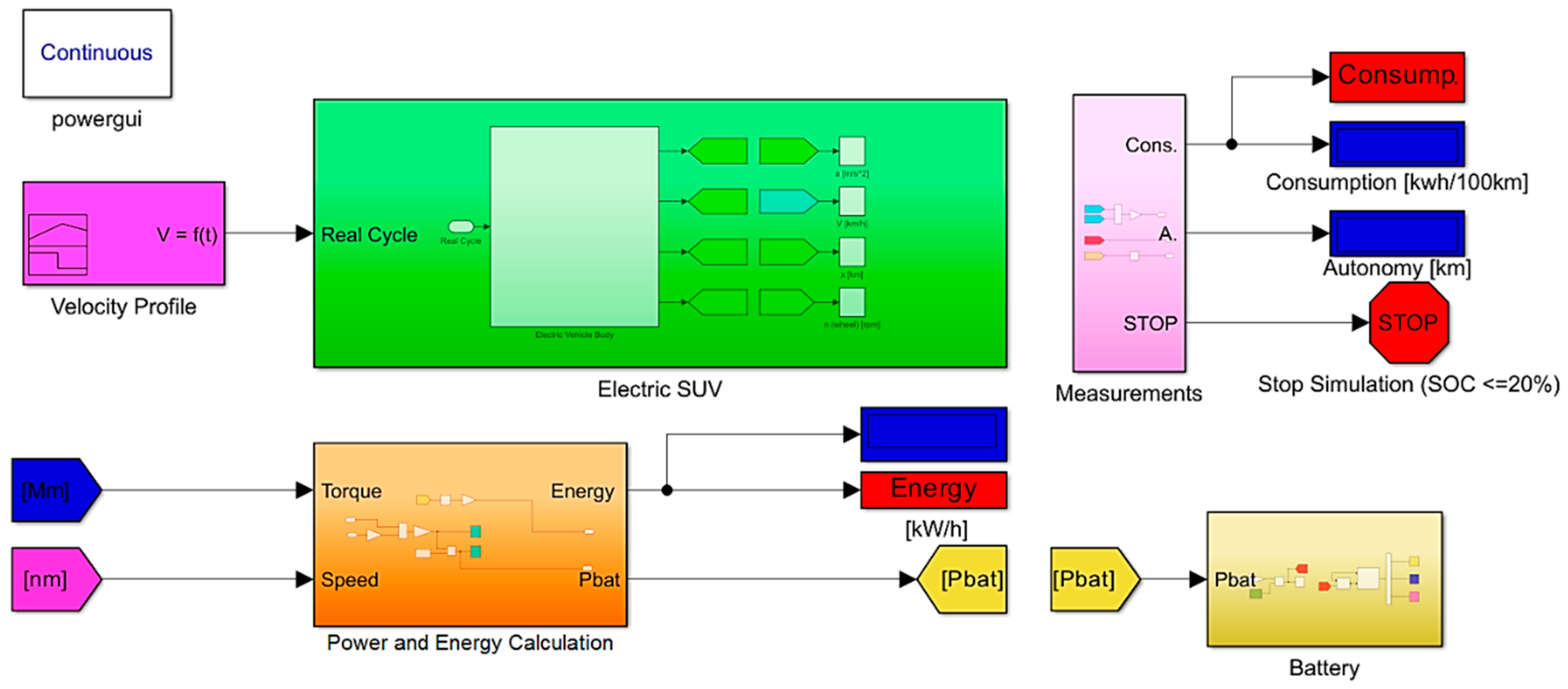
Figure 5.
WLTC velocity profile.
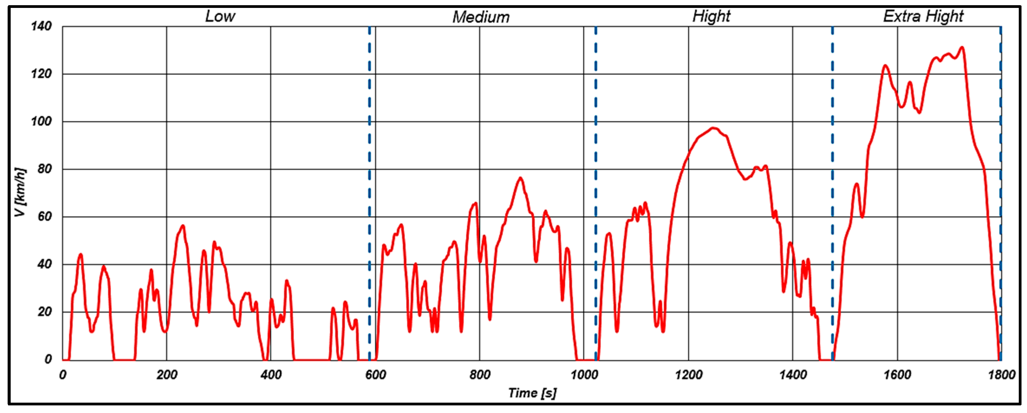
Figure 6.
Velocity profile obtained from experimental measurements: 1 – Urban phase; 2 – Extra-urban phase; 3 – Highway phase.
Figure 6.
Velocity profile obtained from experimental measurements: 1 – Urban phase; 2 – Extra-urban phase; 3 – Highway phase.
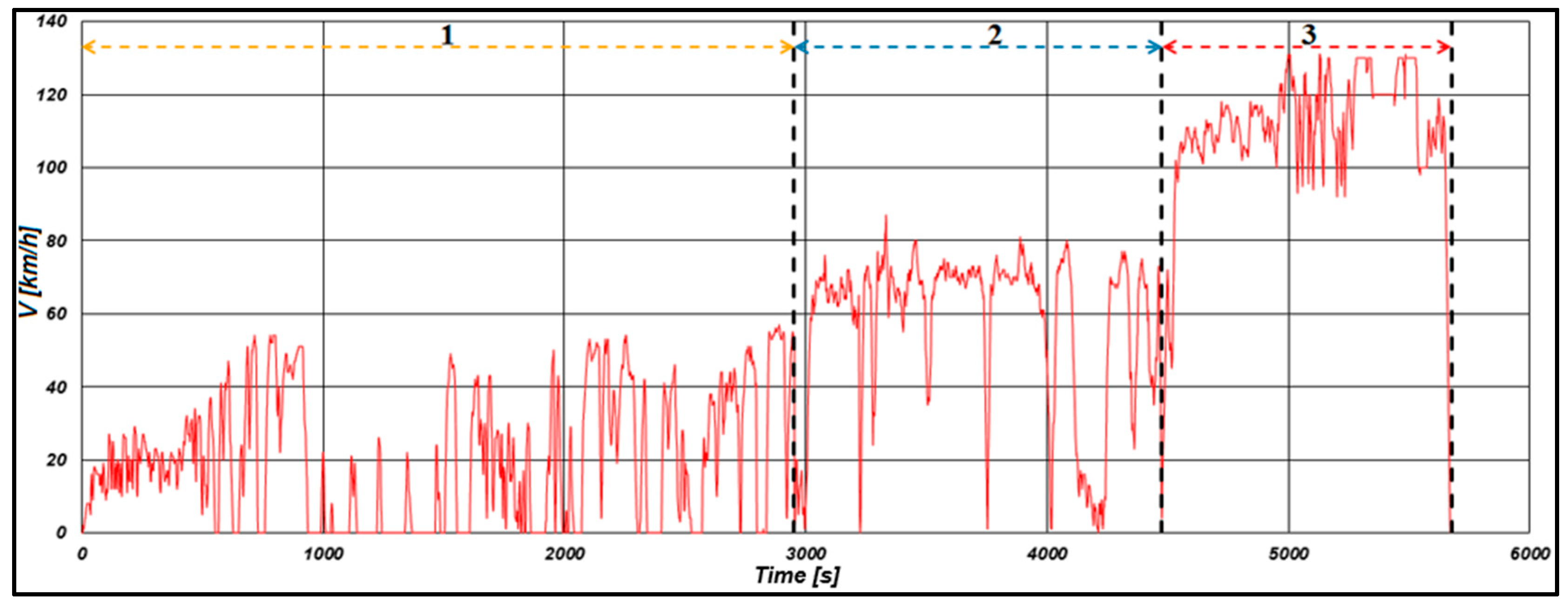
Figure 7.
Variation of the acceleration during the cycle.
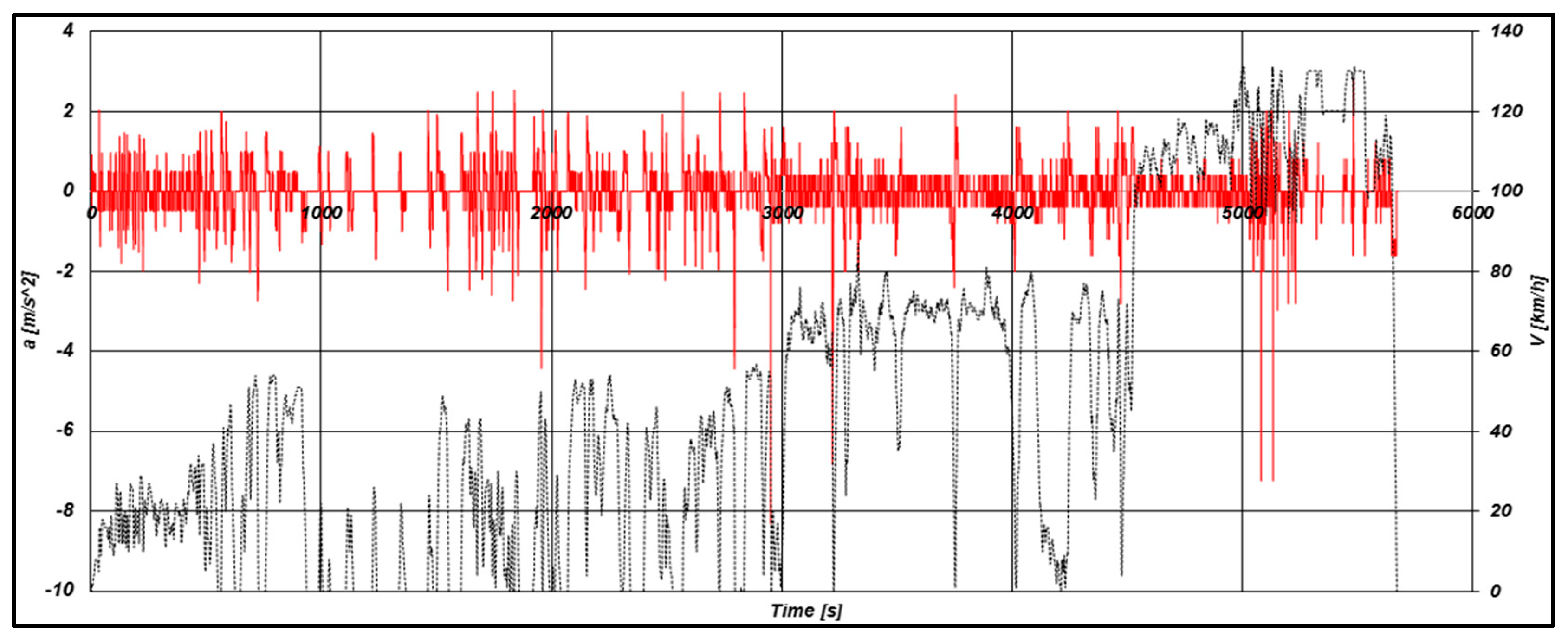
Figure 8.
Battery SOC variation.
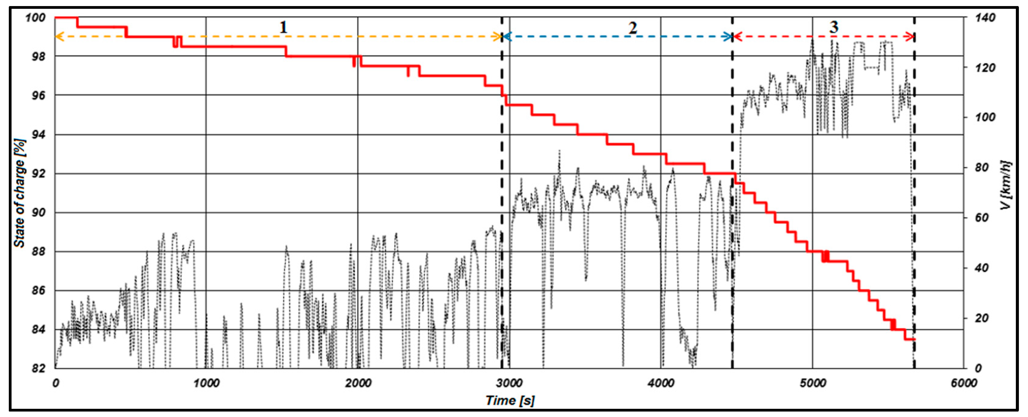
Figure 9.
Variation of total energy during the cycle.
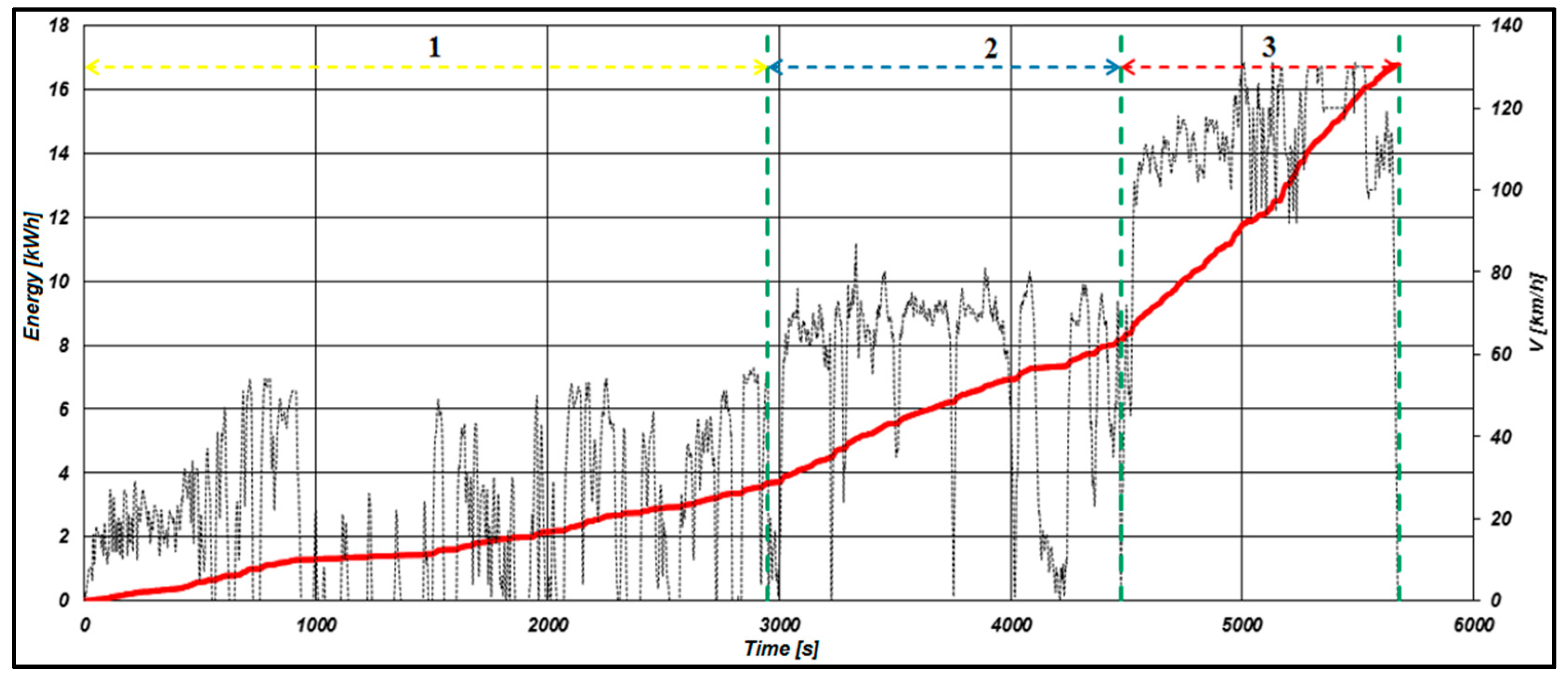
Figure 10.
The variation of energy consumption during the cycle.
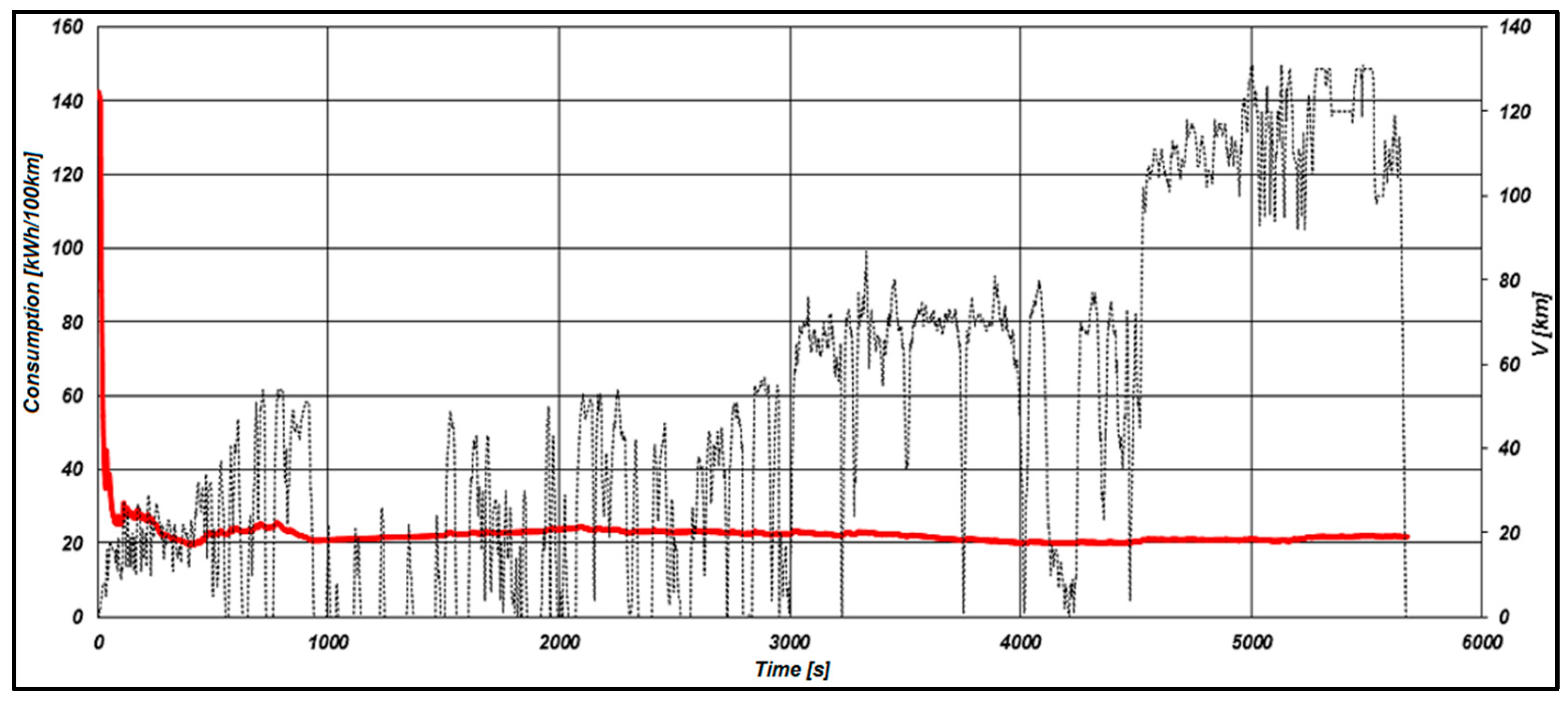
Figure 11.
Velocity profiles.
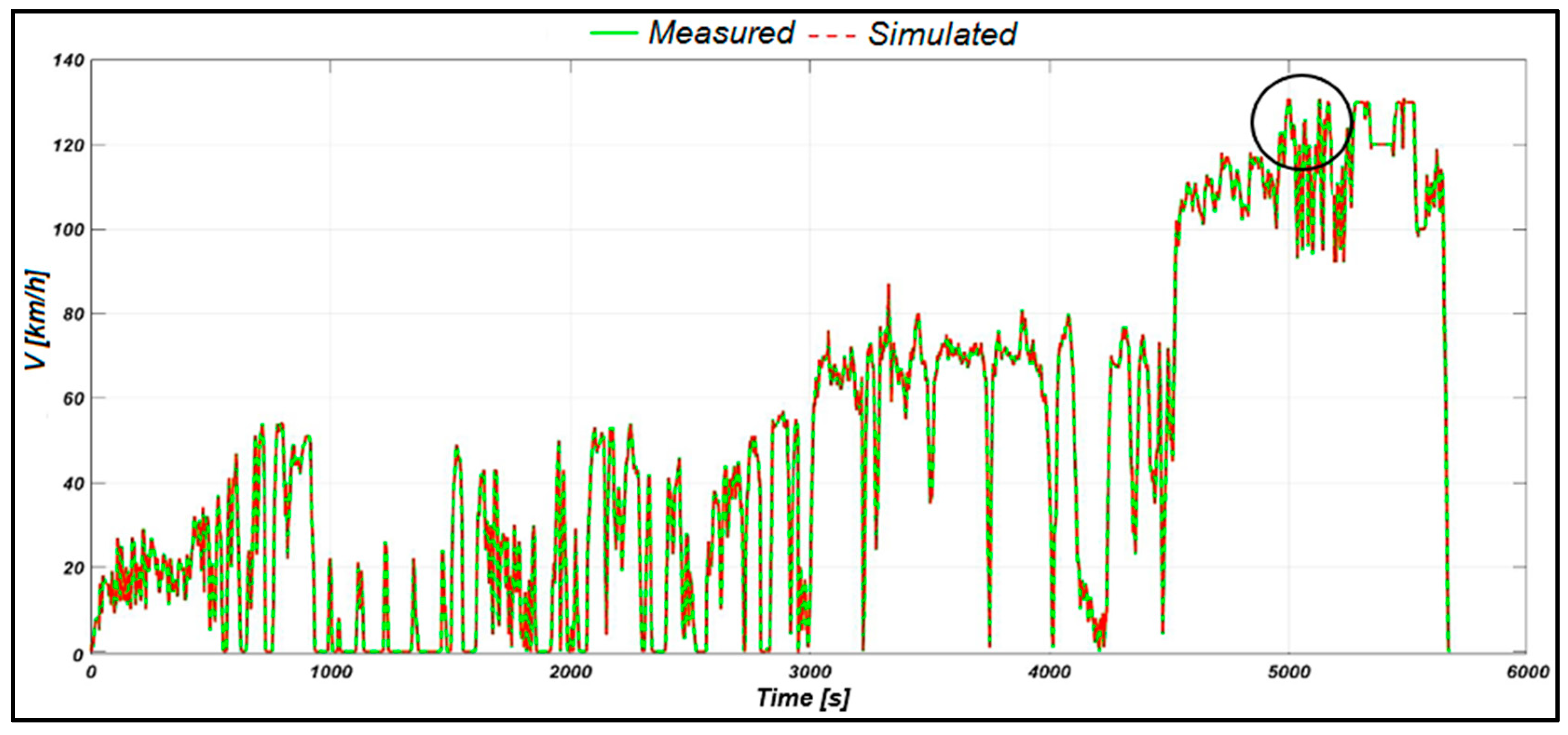
Figure 12.
Velocity profiles.
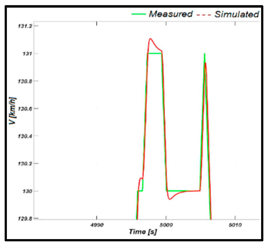
Figure 13.
State of charge variation.
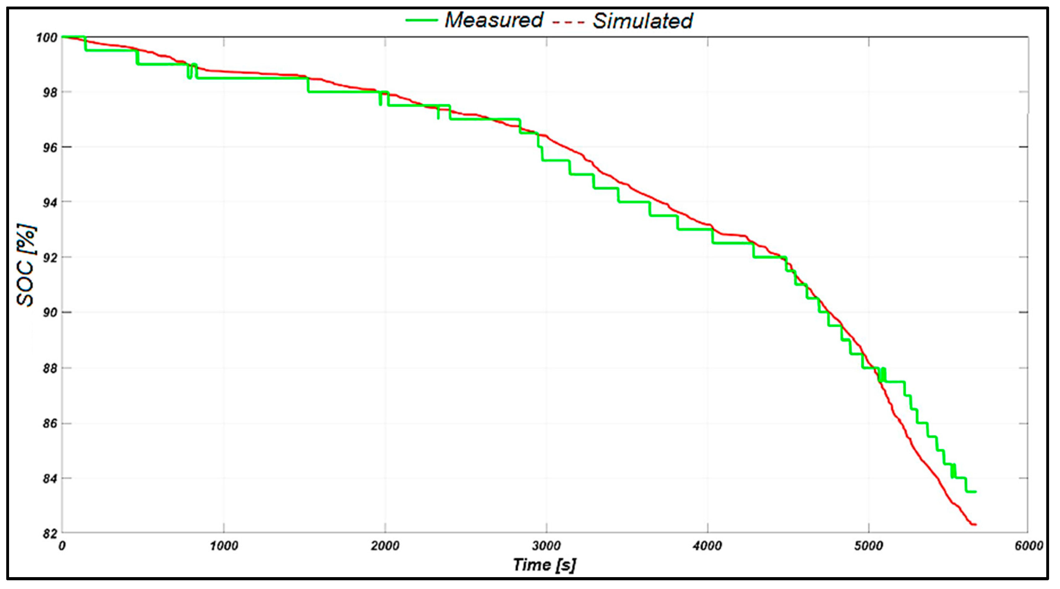
Figure 14.
Energy variation.
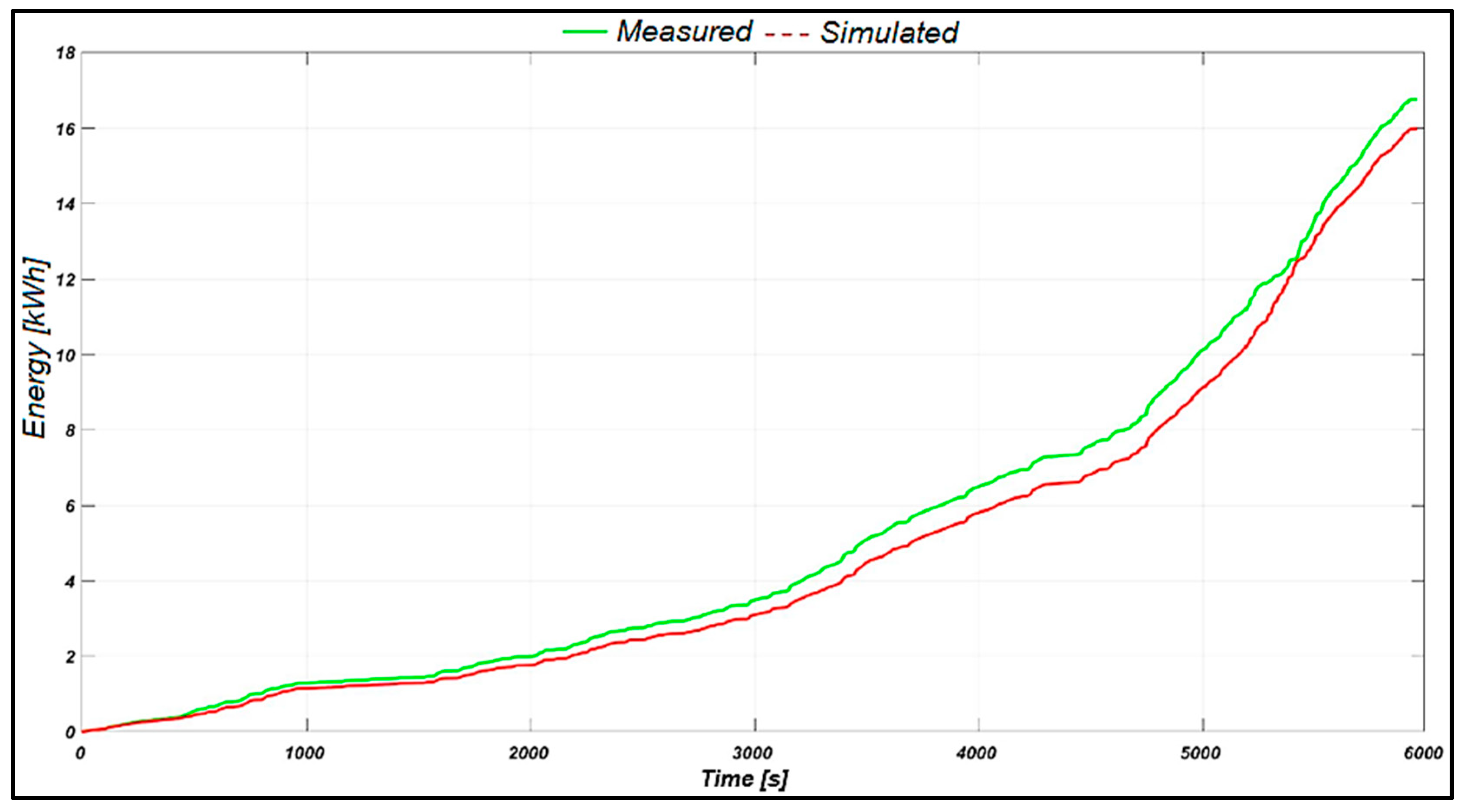
Figure 15.
Energy consumption variation.
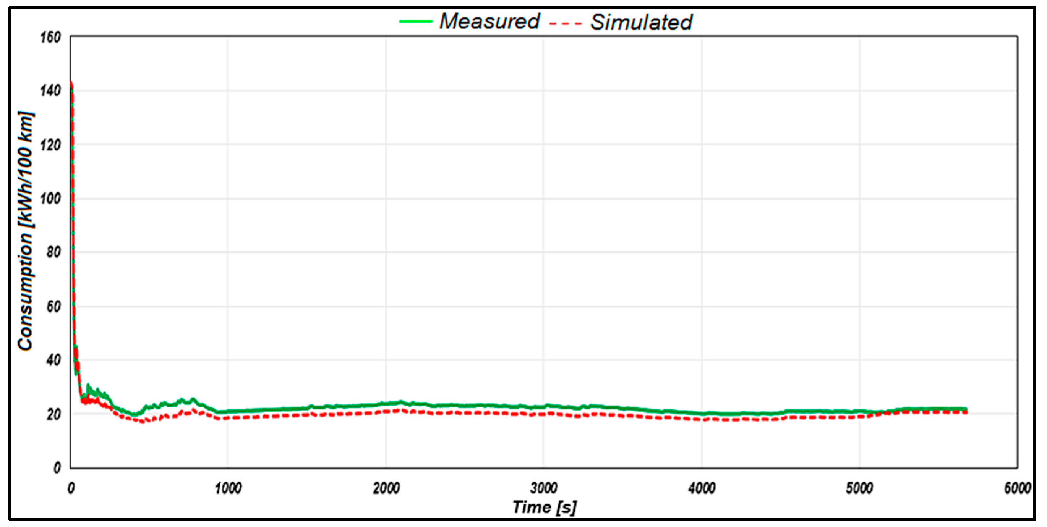
Figure 16.
Real – simulated speed profile comparison for WLTC.
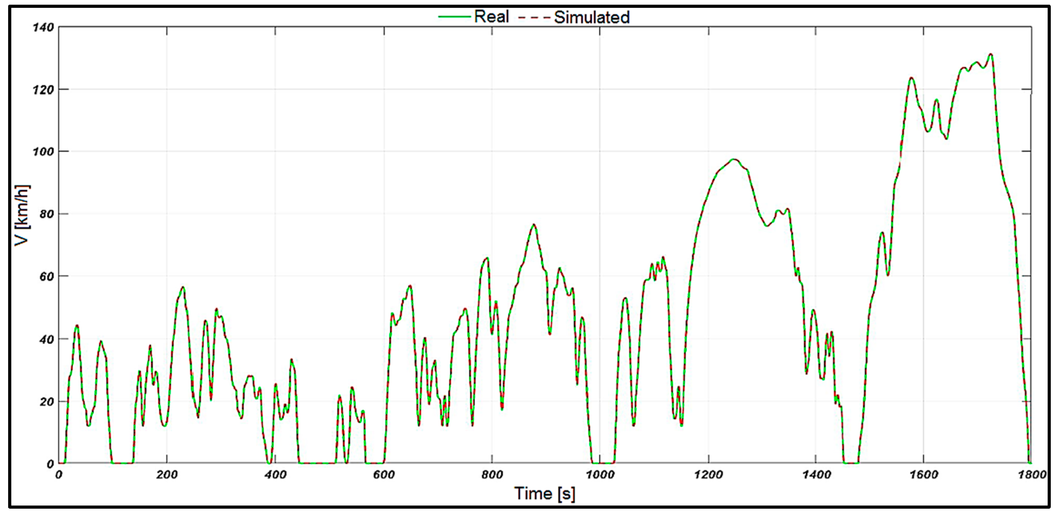
Figure 17.
Real – simulated acceleration profile comparison for WLTC.
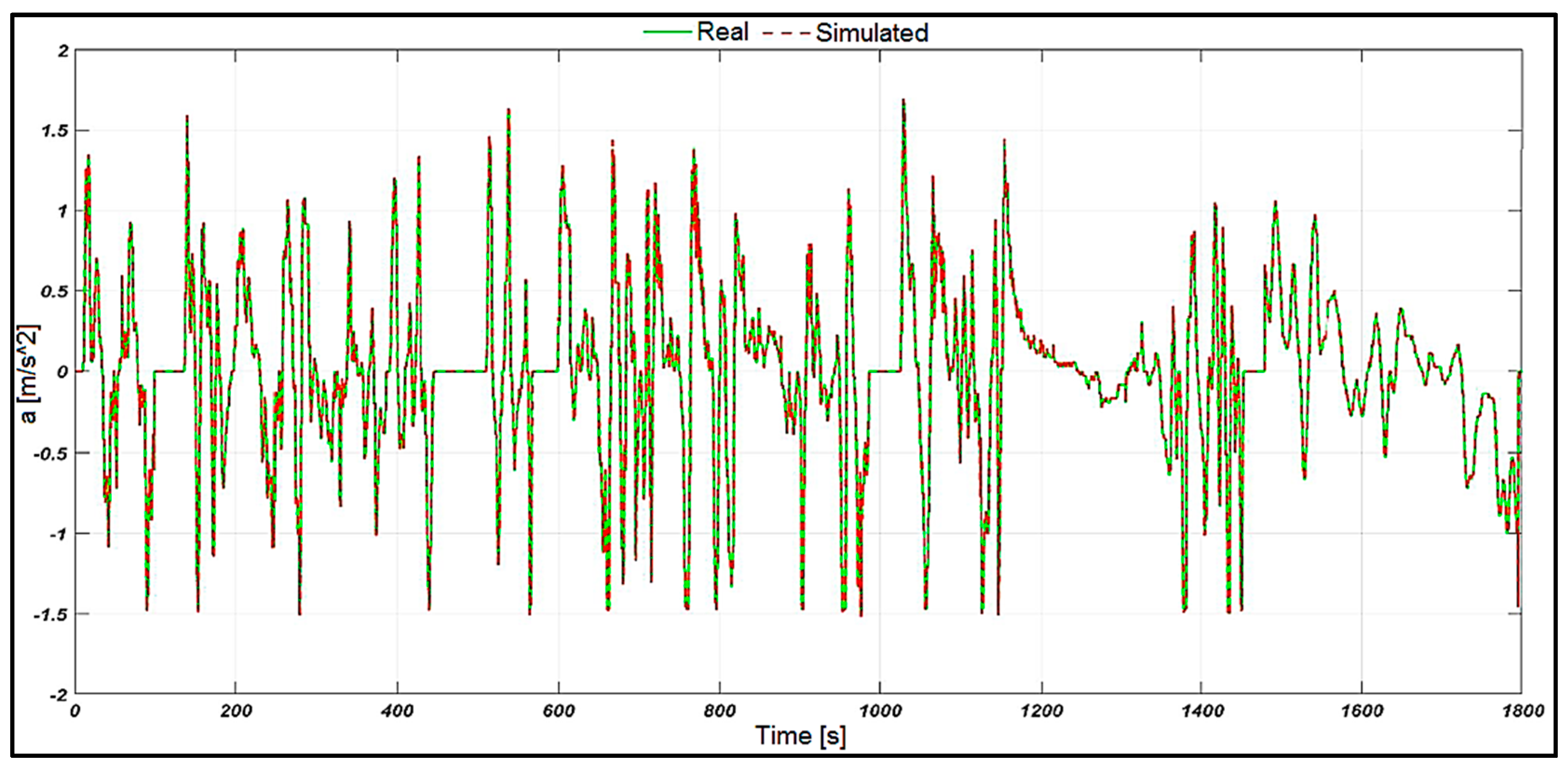
Figure 18.
Simulated SOC for WLTC.
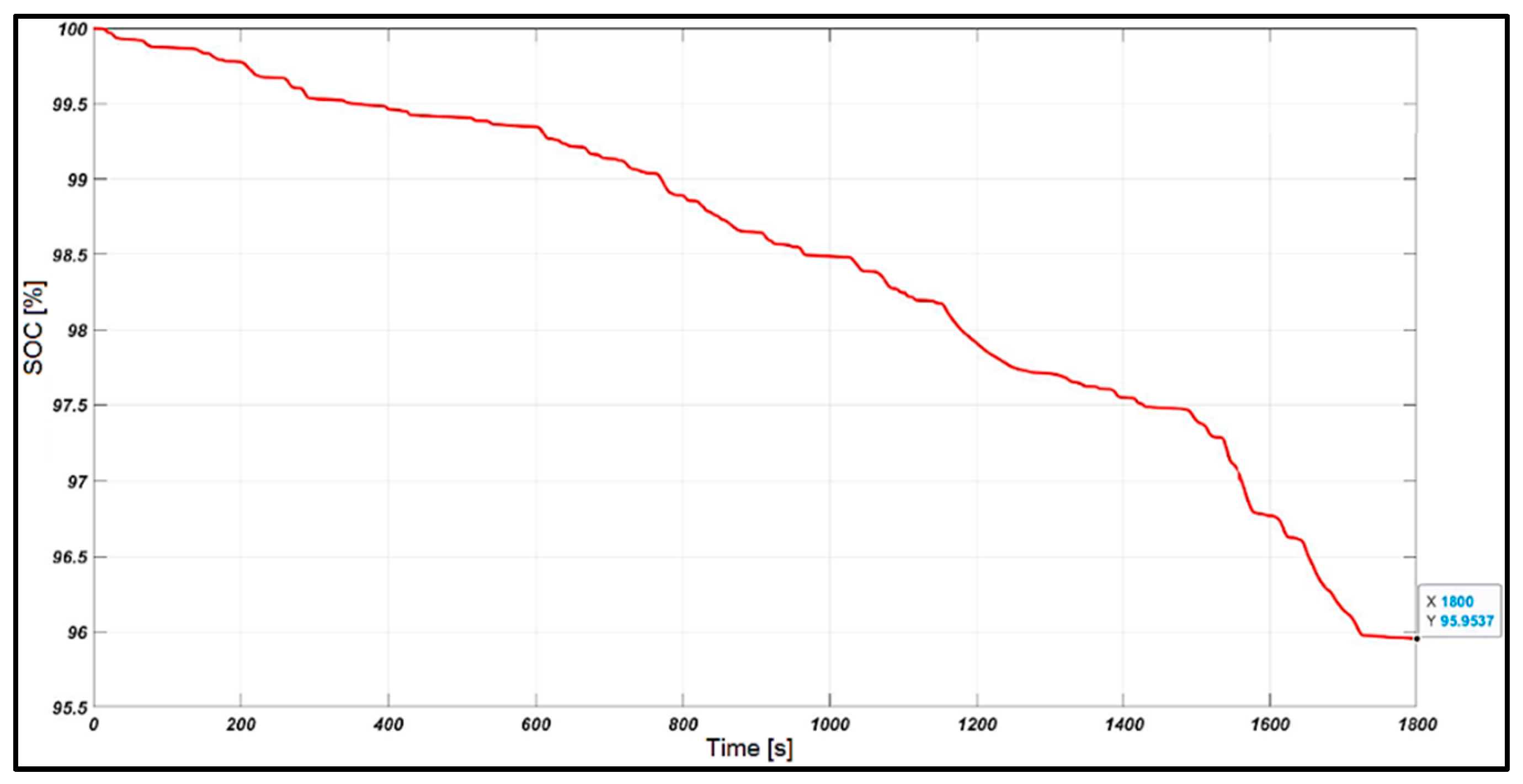
Figure 19.
Simulated energy for WLTC.
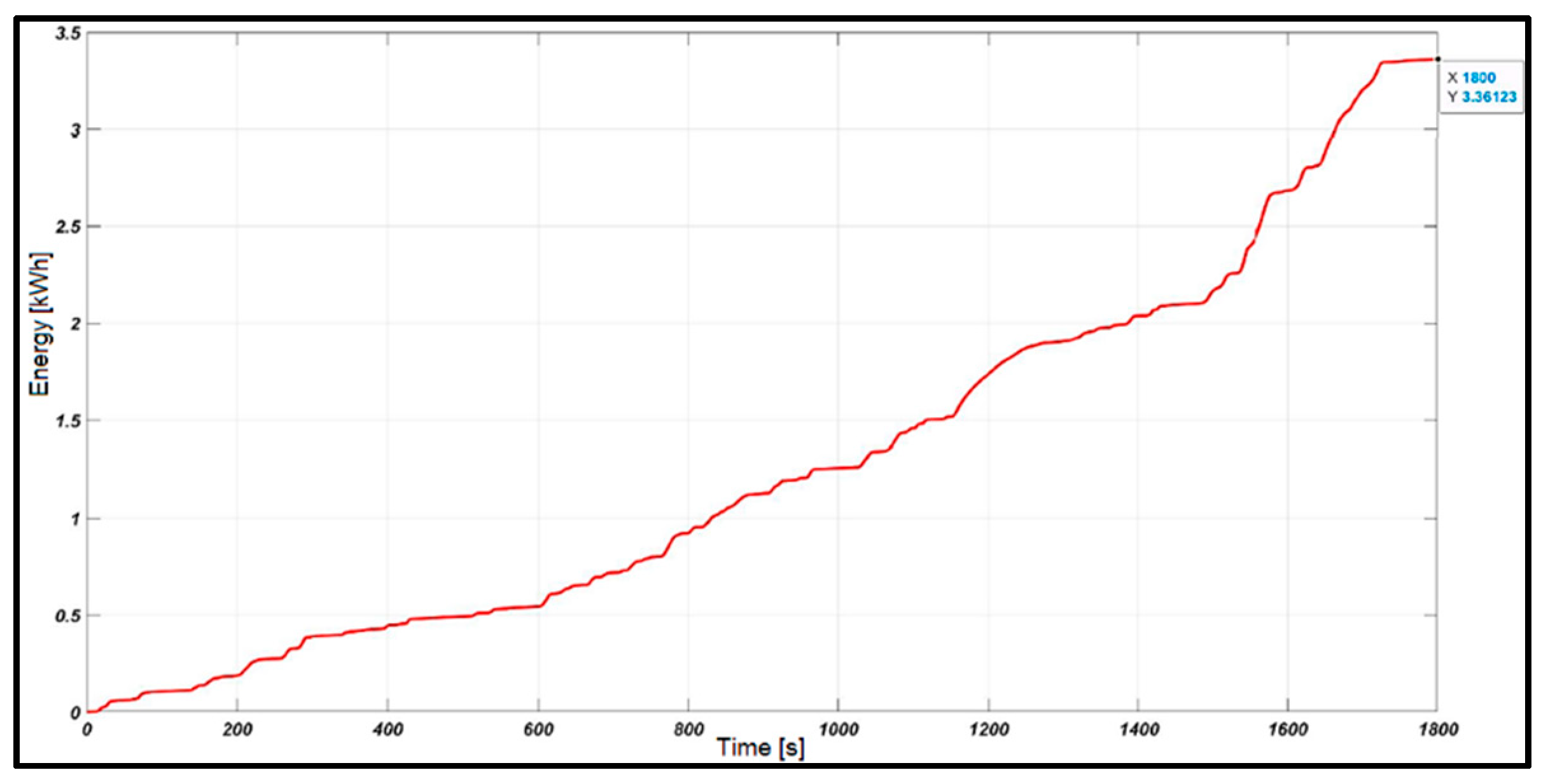
Figure 20.
Simulated consumption for WLTC.
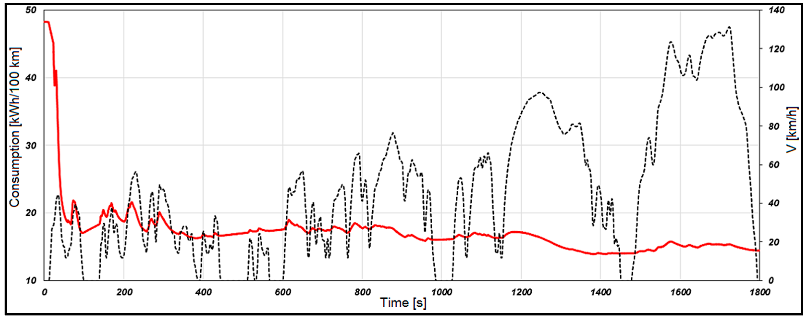

Table 1.
Electric SUV parameters [2].
Table 1.
Electric SUV parameters [2].
| Name | Value | Unit |
|---|---|---|
| Vehicle mass, m | 2325 | kg |
| Max. velocity, V | 160 | km/h |
| Frontal area, A | 2.5 | m2 |
| Drag coefficient, cx | 0.258 | - |
| Rolling radius, rr | 0.356 | m |
| Total gear ratio, it | 13 | - |
Table 2.
Electric motor parameters [2].
Table 2.
Electric motor parameters [2].
| Name | Value | Unit |
|---|---|---|
| Power, Pm | 150 | kW |
| Torque, Mm | 310 | Nm |
| Torque speed, nM | 0…4500 | rpm |
| Max. speed, n | 16000 | rpm |
Table 3.
Traction battery parameters [2].
Table 3.
Traction battery parameters [2].
| Name | Value | Unit |
|---|---|---|
| Initial SOC | 100 | % |
| Nominal voltage, U | 355 | V |
| Total energy, Etotal | 82 | kW |
| Usable energy, Eusable | 77 | kW |
| Capacity, C | 234 | Ah |
Table 4.
Simplifying conditions.
| Name | Value | Unit |
|---|---|---|
| Road inclination, αp | 0 | ° |
| Ambient temperature, t | 10 | °C |
| Propulsion systems efficiency, η | 0.94 | - |
Table 5.
WLTC characteristics [9].
Table 5.
WLTC characteristics [9].
| Name | Value | Unit |
|---|---|---|
| Distance | 23.3 | km |
| Time | 1800 | s |
| Phases | 4 | - |
| Maximum velocity | 131.1 | km/h |
| Medium velocity | 46.5 | km/h |
| Maximum acceleration | 1.7 | m/s2 |
Table 6.
Energy consumption comparison.
| According to manufacturer | Real (measured) | Difference | Relative error |
|---|---|---|---|
| 22.9 | 21.78 | 1.12 | 4.89 |
| kWh/100km | kWh/100km | kWh/100km | % |
Table 7.
Autonomy comparison.
| According to manufacturer | Real (measured) | Difference | Relative error |
|---|---|---|---|
| 337 | 373.3 | 36.3 | 10.7 |
| km | km | km | % |
Table 8.
Autonomy comparison.
| Speed deviation | Max. motor speed | Max. acceleration | SOC | Total energy | Energy consumed by auxiliary systems | Consumption | Autonomy |
|---|---|---|---|---|---|---|---|
| +0.015/-0.021 | 12720 | 1.694 | 95.95 | 3.36 | 0.35 | 14.49 | 512 |
| km/h | rpm | m/s2 | % | kWh | kWh | kWh/100km | km |
Disclaimer/Publisher’s Note: The statements, opinions and data contained in all publications are solely those of the individual author(s) and contributor(s) and not of MDPI and/or the editor(s). MDPI and/or the editor(s) disclaim responsibility for any injury to people or property resulting from any ideas, methods, instructions or products referred to in the content. |
© 2024 by the authors. Licensee MDPI, Basel, Switzerland. This article is an open access article distributed under the terms and conditions of the Creative Commons Attribution (CC BY) license (http://creativecommons.org/licenses/by/4.0/).
Copyright: This open access article is published under a Creative Commons CC BY 4.0 license, which permit the free download, distribution, and reuse, provided that the author and preprint are cited in any reuse.


