
Submitted:
06 June 2025
Posted:
09 June 2025
You are already at the latest version
Abstract
Dual-motor electric vehicles enhance power performance and overall output capability by enabling real-time control of torque distribution between the front and rear wheels, thereby improving handling, stability, and safety. In addition to increased energy efficiency, a dual-motor system provides redundancy, if one motor fails, the other can still supply partial power, further enhancing driving safety. This study aims to optimize the energy management strategies of front and rear axis motors, examining the application effects of rule-based control (RBC), global grid search (GGS) and whale optimization algorithm (WOA). A simulation platform based on Matlab/Simulink® was constructed and validated through hardware-in-the-loop (HIL) testing to ensure the authenticity and reliability of simulation results. Detailed tests and analyses of the dual-motor system were conducted under FTP-75 driving cycles. Compared to the RBC strategy, GGS and WOA achieved energy efficiency improvements of 9.1 % and 8.9 %, respectively, in pure simulation; and 4.2 % and 3.8 %, respectively, in HIL simulation. Overall, GGS and WOA each present distinct advantages, with WOA emerging as a highly promising alternative energy management strategy. Future research should further explore WOA applications to enhance energy savings in real-world vehicle operations.
Keywords:
whale optimization algorithm
; electric vehicle
; dual-motor
; global grid search
; hardware-in-the-loop
1. Introduction
In today's era of rapid technological advancement, scientists are actively developing innovative energy solutions to address the threats of climate change and resource depletion [1]. The acceleration of industrialization and the resulting global population growth have driven the development of urban areas, posing challenges to providing convenient and livable environments for people [2]. As an indispensable part of modern society, transportation profoundly impacts economic efficiency and the sustainable development of society [3]. Automobiles, airplanes, and trains not only offer fast and convenient transportation but have also become an essential part of modern society. However, the energy demands of these modes of transport have emerged as a major challenge today [4]. The advent of mass vehicle production triggered an explosive growth in global transportation, accompanied by significant greenhouse gas emissions. This not only posed a serious threat to the Earth's ecological environment but also raised concerns about the depletion of limited energy resources [5]. The energy demands of human society have continued to grow at an increasing rate. This situation has compelled countries around the world to reconsider their approaches to energy usage, strengthen the development and application of environmental technologies, and promote environmental protection and energy sustainability [6]. The development of renewable energy, improvement of energy efficiency, and advancement of transportation technologies have become key components in achieving green mobility, while also reducing the pressure on the Earth's resources [7]. With the rapid advancement of technology, energy management in transportation will continue to be a focal point of technological innovation and sustainable development [8]. Future vehicle research will primarily focus on three major directions: battery electric vehicles (BEVs), hybrid electric vehicles (HEVs), and hydrogen fuel cell electric vehicles (FCEVs) [9]. Among these, BEVs are considered one of the primary global development objectives. In response to the energy crisis and environmental challenges, major automotive manufacturers are progressively adjusting their research and development directions, actively promoting innovations in new energy technologies. This shift not only demonstrates a commitment to sustainable development but also significantly reshapes the competitive landscape of the automotive industry [10].
Recently, automotive manufacturers and governments worldwide have actively committed themselves to developing new energy vehicles. This has made the evolution from traditional internal combustion engine vehicles to HEVs a prominent trend. Major automakers have successfully developed hybrid vehicles with dual power outputs by combining internal combustion engines with electric drive motors [11]. This system utilizes two or more power sources to drive the vehicle and can flexibly switch between them under various conditions, thereby achieving optimal performance across different driving scenarios [12]. This technology not only extends the driving range of vehicles but also reduces energy consumption, bringing hybrid vehicles closer to the performance level of new energy vehicles. This development direction holds great promise for achieving energy-saving and carbon-reduction goals, offering a more forward-looking and environmentally friendly transportation solution to support sustainable development in the future [13]. According to previous studies, the primary goals of optimizing energy and power systems are energy conservation and cost reduction. In this context, energy management strategies and power system design have become two critical considerations in related research. Among them, energy management strategies play a pivotal role in the optimization of energy and power systems [14]. Through proper energy management, the system can more effectively utilize the conversion between different energy sources, thereby achieving more energy-efficient and environmentally friendly operation. The design of the electrical/power system directly affects the performance of the hybrid energy system. [15]. Selecting appropriate power components, energy storage devices, and power transmission network structures ensures the coordinated operation of the entire system, achieving optimal performance [16].
The power system of BEVs can be divided into two main configurations: (1) single-motor drive and (2) multi-motor drive. The single-motor configuration features a simplified structure and the use of high-performance electric motors, which makes it more challenging to balance vehicle performance with improved energy efficiency [17]. Multi-motor drive systems can be further categorized into two types based on the number of motors: (1) four-motor distributed drive and (2) dual-motor coupled powertrain [18]. The four-motor distributed drive system features individual motors assigned to each wheel, with each wheel delivering power independently through separate reducers or drive shafts, or alternatively, integrating motors directly into the wheels as hub motors [19]. In contrast, the dual-motor coupled powertrain employs two motors to achieve multiple driving modes. Through an ingeniously designed mechanical coupling mechanism, the system efficiently allocates power between the two motors, significantly enhancing motor utilization. Compared to conventional single-motor setups, this configuration achieves superior overall performance [20].
According to previous studies, optimization of a vehicle's energy management system primarily aims at reducing overall energy consumption and lowering costs to enhance overall efficiency and system performance. Energy management system strategies can mainly be categorized into two types: (1) rule-based (RB) strategies and (2) optimization-based strategies [21]. Rule-based strategies can be further divided into two main types: (1) deterministic rules and (2) fuzzy logic rules [22]. Deterministic rules involve predefined control strategies based on engineering experience to manage switching between different operational modes of the powertrain and distributing power among various energy sources [23]. In contrast, fuzzy logic rules employ a set of predetermined yet flexible control strategies, allowing more adaptable handling of uncertainties and complexities within the system. Decisions and controls are executed through fuzzy logic, enabling dynamic adjustments to operational modes and power allocation between different energy sources [24]. Optimization-based strategies can be mainly classified into two categories: (1) real-time optimization and (2) global optimization [25]. Real-time optimization involves dynamically allocating power between the engine and electric motor based on current power demands, ensuring the minimum equivalent consumption and minimal power losses at each moment. An example of this approach is the global grid search (GGS) [26]. Global optimization utilizes optimal control principles to improve fuel consumption and power loss across an entire driving cycle, dynamically optimizing power allocation among energy sources to achieve overall optimal vehicle performance. Examples include methods such as dynamic programming (DP) [27] and genetic algorithm (GA) [28]. To thoroughly investigate vehicle energy efficiency, this research primarily focuses on two main areas: the powertrain system and the control strategy. Regarding powertrain design, recent commercially available vehicles exhibit highly similar system architectures, with multi-power-source configurations emerging as the mainstream design. In terms of control strategies, theory-based controls have already achieved considerable success in various engineering applications. Currently, bio-inspired heuristic algorithms, such as the whale optimization algorithm (WOA), are gradually becoming a popular trend in the field of optimization methods [29].The WOA compared with other heuristic algorithms, demonstrates superior problem-solving capabilities and computational efficiency. It is feasible for energy management involving multiple control variables, thereby enhancing the performance of hybrid power systems and showcasing its significant potential in vehicle control applications [30].
To effectively validate the practical operation of the energy management system, a HIL system is utilized to perform real-time computation, bridging the gap between the simulation phase and actual vehicle implementation. This approach helps identify data errors and enhances system fault tolerance. In this research, the dual-motor drive simulation platform is divided into two parts: the vehicle control unit (VCU) and the vehicle platform. An Arduino DUE microcontroller and a Ti C2000 microcontroller are employed to construct a hardware-in-the-loop (HIL) platform, enabling analog and digital input/output signal conversions through signal processing. The FTP-75 (Federal Test Procedure 75) driving cycle is used as a basis for analyzing the performance characteristics and inter-system response relationships, including torque, rotational speed, optimization management, and overall vehicle energy efficiency.
2. Establishment of a Vehicle Dynamics Model
2.1. Electric Vehicle Simulation Platform
The objective of this study is to establish a dual-motor drive system, using a high-chassis Tesla Model X as the base vehicle specification [31]. The vehicle is equipped with a 95 kW ZEPT drive motor integrated with a gearbox, provided by ZEPT (Zero Emission Power Train), a company based in Taoyuan City, Taiwan, specializing in complete electrification solutions for mobile vehicles.. The motor specifications are proportionally scaled according to power requirements [32]. Finally, power distribution is optimized through control strategies, as shown in Table 1. Specification of the electric vehicle. This paper adopts a dual-motor drive system architecture, with the vehicle system featuring an independent suspension design for both the front and rear axles. The model is based on test data from the dual motors and lithium battery pack of the actual vehicle model (Tesla model X). The detailed structure is shown in Figure 1.
This study focuses on the optimization of energy management strategies to evaluate the rationality of motor power distribution and performance data through comparative analysis. The drive motors transmit power to the vehicle’s wheels via gearboxes, and a vehicle velocity tracking simulation model is used for detailed analysis. First, the velocity error is calculated as the difference between the driving cycle velocity and the actual vehicle velocity. A PI controller is then used to compute the demanded vehicle torque, and the resulting signal is sent to the optimized energy management system. Considering the demanded vehicle velocity and the battery's state of charge (SOC), an optimization algorithm is applied to determine the total demanded torque. In this study, the vehicle simulation platform is built using Matlab/Simulink® (R2021b, MATLAB, Natick, MA, USA), as shown in Figure 2. The platform includes the following models: driving cycle, driver, motor, battery, vehicle dynamics, and energy management system.
2.2. Driving Cycle Model
The FTP-75 is a standardized testing procedure mandated by the U.S. environmental protection agency (EPA) for evaluating vehicle fuel efficiency. It simulates both urban and highway driving conditions and uses these conditions to calculate a vehicle’s fuel consumption and emission data [33]. The FTP-75 test procedure includes a series of predetermined driving cycles, velocity, and idle periods to reflect the vehicle's performance in real-world usage scenarios. In this study, the FTP-75 test cycle with a total driving time of 1370 s and a maximum velocity of approximately 90 km/h is adopted, as shown in Figure 3.
2.3. Driver Model
Proportional-integral (PI) control is a commonly used type of control system in engineering. It combines proportional control (P) and integral control (I) to improve the response velocity and accuracy of the control system, resulting in better overall performance [34]. By integrating both proportional and integral components, the controller can respond quickly to error changes while eliminating steady-state error, ensuring that the final output reaches the demanded set point. In the vehicle simulation, the actual vehicle velocity and the demanded velocity are calculated and subtracted to obtain the velocity error, which is then used as input to the driver model. The output of the PI controller provides the total demanded torque and braking torque to appropriately adjust the vehicle’s demanded power, as expressed by the following Equation (1):
Where is the total demanded torque; is the gain constant of proportional control; is the gain constant of integral control; is the velocity error.
2.4. Drive Motor Model
In this study, the drive motor model receives the demanded drive torque output from the driver model, considering the motor’s maximum physical speed limitation, computes the feasible torque and delivers the appropriate drive torque for vehicle propulsion. The mechanical efficiency curve of the drive motor is shown in Figure 4. Motor efficiency is determined using a two-dimensional lookup table based on the current motor speed and torque. The efficiency calculation is represented by Equation (2):
Where is the efficiency of the drive motor; is the output torque of the drive motor; is the speed of the drive motor.
2.5. Energy Storage Battery Model
The lithium battery serves as the primary power source for the vehicle’s drive motors. Based on real-world data obtained from the lithium battery, a relationship was established between the internal resistance and voltage, which can be used to estimate the battery's SOC. In the model developed for this study, the battery temperature is assumed to be constant and does not vary with operating conditions or duration. The accuracy of the battery's SOC estimation is critical, as it significantly influences the vehicle’s dynamic performance and is one of the key parameters in energy management strategies. This study adopts an internal resistance model, in which the battery contains an equivalent , which varies with the battery’s and temperature , as expressed in Equation (3):
Where is the internal resistance value of the battery; is the battery’s state of charge; is the temperature of the battery.
The variation in battery state exhibits a first-order dynamic response. The SOC ranges from 0 to 1 (0–100%). This relationship is expressed by Equation (4):
Where is the rated capacity of the lithium battery; is the discharge current of the battery; is the charge-discharge efficiency of the battery. is a function of the relationship between and :
The discharge current of the battery calculation method is as shown in Equation (6):
Where is the open circuit voltage of the battery, a function of and ; is the discharge power of the battery to the drive motor. The calculation method for the load voltage of the battery during discharge is shown in Equation (7):
The dynamic performance of the battery resistance is calculated using the internal resistance method. Based on experimental data from individual energy storage cells, the variation in internal resistance under different SOC conditions can be estimated. This allows for the determination of the open circuit voltage (OCV) values corresponding to different SOC.
2.6. Vehicle Dynamics Model
The vehicle dynamics model is a critical component of the entire system, used to simulate the vehicle's dynamic behavior under various driving conditions. When analyzing driving scenarios, it is essential to consider various forms of resistance. The vehicle’s traction force is equal to the sum of the forces acting in the direction opposite to its motion. During operation, the vehicle primarily encounters three types of resistive forces: air resistance, rolling resistance, and gradient resistance. These forces are closely related to the vehicle's performance and operation. The vehicle's acceleration force is equal to the driving force minus the air resistance, gradient resistance, rolling resistance and braking force, these forces can be expressed by the Equation (8):
Where is the drag coefficient; is the frontal area of the electric bus; is the air density; is the vehicle velocity; is the total vehicle mass; is the rolling resistance coefficient; is the gravitational acceleration; is the gradient angle.; is the output torque of the final drive; is the overall efficiency of the final drive; is the braking force.
2.7. Hardware in-the-loop System Architecture
In the development process of this study, the HIL system plays a critical role as an indispensable tool to ensure that the product operates smoothly before entering mass production. Through this system, the functionality and feasibility of the controller can be verified in advance to assess whether it meets the expected performance [35]. This helps identify potential issues early, allowing for timely corrections that reduce the cost of later-stage problem-solving, while also ensuring product safety and functional reliability. It also allows observation of whether output results exhibit distortions or delays that need to be addressed. This step is essential in the phase prior to technological development and commercialization, facilitating faster and more accurate debugging [36]. In this study, the HIL system platform was built using an Arduino DUE microcontroller and a TI C2000 microcontroller. Both the real-time model of the full vehicle platform and the real-time model of the vehicle controller were developed using Matlab/Simulink® software. These models simulate the operation of the entire vehicle system in real time and allow for immediate computation and validation to ensure optimal vehicle performance under various conditions. As shown in Figure 6, the driving cycle provides the demanded vehicle velocity to the driver model. The PI controller then outputs the demanded vehicle torque. Simultaneously, the battery model calculates the battery's SOC, and the vehicle dynamics model computes the motor output speed. These three outputs are transmitted to the receiving end of Figure 5. Through the energy management strategy, power is distributed to the front axis motor, rear axis motor, and the power distribution ratio, then sent back to the receiving end in Figure 6. During this signal transmission process between the two models, the system continuously converts the vehicle's digital signals into voltage signals, and then converts these voltage signals back into the digital signals required by the vehicle, ensuring smooth communication between the two systems at all times.
In this study, the Ti C2000 microcontroller is connected to the Arduino DUE microcontroller to perform HIL system testing. The HIL system architecture is shown in Figure 7. To verify the authenticity of the dual-motor drive power system, the setup is divided into two parts: the real-time model of the vehicle platform and the real-time model of the VCU. This division allows for better control and testing of each component of the system, ensuring performance and reliability under real-world applications. Before performing signal processing, it is necessary to understand how analog signals are converted into voltage by the Arduino DUE and Ti C2000. The Arduino DUE converts analog signals ranging from 0.56 to 2.76 V into digital values ranging from 0 to 4095, while the Ti C2000 converts analog signals from 0 to 3.3 V into the same digital range 0 to 4095. The Arduino DUE is a feature-rich microcontroller, whereas the Ti C2000 series is a high-performance microcontroller designed specifically for control applications. Due to the differences in voltage handling between the two microcontrollers, proportional amplification or attenuation is required, as shown in Table 2. The system's pin assignments include demanded torque, battery SOC, and target speed. These are output from the Arduino DUE and, after signal conversion, serve as input to the Ti C2000. The Ti C2000 then performs optimized calculations based on the energy management strategy and outputs the demanded signals, including the motor power distribution ratio, the front demanded motor torque, and the rear demanded motor torque. These signals are then converted and sent back to the Arduino DUE as input signals, as summarized in Table 2.
3. Energy Management Strategy
This study adopts an energy management strategy to calculate the optimal motor efficiency range and determine the best power distribution ratio. Simulation verification is conducted using the FTP-75 driving cycle, and the control architecture of the energy management system is illustrated in Figure 8. First, the driving cycle model provides the target vehicle velocity for simulation. The actual vehicle velocity is then calculated through the vehicle dynamics model. The vehicle velocity error, obtained by subtracting the actual velocity from the demanded vehicle velocity, is used as the input to the PI controller. The PI controller outputs the demanded torque, which is sent to the energy management model to determine the power distribution between the dual drive motors. Meanwhile, the braking torque is used to command the braking force and is sent to the vehicle dynamics model to perform vehicle braking. The energy management model uses the actual motor speed from the vehicle dynamics model to calculate the optimal torque distribution, sending control commands to the front and rear axis motors for execution. Finally, the motor outputs are integrated into the vehicle dynamics model to compute the actual vehicle velocity.
3.1. Rule-based Control Strategy
Rule-based control (RBC) is implemented using the Stateflow model in MATLAB/Simulink® to develop the energy management strategy. Based on different driving demands, corresponding power distribution modes are established, as detailed in Table 3. When the input signals meet the predefined state conditions, the system outputs the corresponding power distribution results. These rules are primarily formulated based on the researcher’s engineering experience and the operational efficiency of individual components, enabling control over mode switching under various driving conditions [37]. In this study, the RBC strategy defines four operating modes, as shown in Table 3. The mode determination is based on the demanded vehicle velocity, demanded torque, and battery SOC. The modes are defined as follows:
- Ø System Ready Mode: When the driver’s demanded torque is 0 Nm, the system enters the ready mode, and the commanded motor torque output is also set to 0 Nm.
- Ø Low Load Mode: When the demanded torque is greater than or equal to 0.1 Nm, the vehicle enters the low load mode. In this mode, the demanded torque is shared between the front and rear axis motors with a distribution ratio of 3:7.
- Ø High Load Mode: When the actual vehicle velocity exceeds 50 km/h, the system switches to high load mode. In this mode, the demanded torque is allocated to the rear axis motor, which primarily propels the vehicle.
- Ø Safety Mode: When the demanded torque is 0 Nm and the battery SOC reaches 0, the system enters the safety mode.
- Ø These control rules ensure appropriate power allocation and system response under various operating conditions.
3.2. Global Grid Search Method
In the computational process, system model parameters such as total demanded power, motor speed, and physical constraints are established to construct an optimized power distribution model for control system parameter analysis. This approach effectively simplifies the control model to meet the real-time computing requirements of the HIL system. To obtain the optimal control model parameters, a GGS method is used to find the best parameter solution. By first inputting the necessary parameters such as the demanded torque, drive motor speed and performing discretization, an objective function is defined to identify the optimal power distribution algorithm. The goal is to minimize power consumption, and the minimum value is determined as expressed in Equation (9):
Where is the efficiency of the front axis motor; is the efficiency of the rear axis motor; is the input power the front axis motor; is the input power the rear axis motor; is the optimal cost function; is penalty value. The output power of the front and rear axle motors are calculated as shown in Equations (10) and (11):
By substituting Equations (10) and (11), the result is shown in Equation (12):
The represents the penalty value, when the conditions of a grid search exceed physical constraints, a large penalty value is assigned:
In studies related to the front and rear motor power ratio, it has been observed that when electric vehicles require more acceleration and high-speed operation, the importance of the front-axle motor may increase [38, 39]. The GGS method selects the optimal power distribution by minimizing power consumption based on the vehicle’s real-time operating status and control variables, while also taking vehicle performance requirements into account. This enables the vehicle to achieve the most efficient energy management at different operating points, thereby improving overall energy utilization. The strategy process is as follows:
- Ø The GGS search method involves three nested loops used for globally searching discretized values of demanded torque and motor speed.
- Ø The program uses "if-then-else" conditional statements to evaluate various possible operating modes and then calculates parameters such as the efficiency and torque of the front and rear axis motors.
- Ø Based on the concept of minimum power consumption, the power consumption under different conditions is calculated. For a fixed motor speed and demanded torque, the minimum power consumption under different dual-motor torque distributions can be used to determine the optimal power distribution ratio.
Table 4 lists the relevant parameters for the front and rear axle motors. Based on the design of the optimal objective function, the power distribution ratios are defined according to Equations (14) and (15):
Where is the power distribution ratio 0~1).
Under the same minimum motor power consumption strategy, the optimal motor power consumption is identified using the optimal power distribution loop shown in Figure 9. The discretized variables include the required torque, motor speed, and the front rear axle motor power distribution ratio α, which are used to perform a global search. By calculating the electric power consumption of the front and rear axis motors under different variable conditions, an optimal two-dimensional power distribution map can be derived. The calculation is expressed in Equation (16):
3.3. Whale Optimization Algorithm
In this study, a heuristic optimization algorithm inspired by the foraging behavior of whales, is utilized. WOA simulates the process by which whales search for food perceiving information such as sound and scent in their surroundings to determine the direction and distance of prey, then taking corresponding actions. The algorithm mimics these behaviors to search for optimal solutions [40]. One of the most remarkable features of whales is their unique hunting method known as the bubble-net feeding method. This feeding behavior typically occurs near the ocean surface, where whales create bubbles to trap prey. They form these bubble nets along circular or figure-eight-shaped paths. During the upward spiral, a whale dives to a depth of approximately 12 meters and begins creating spiral-shaped bubbles around the prey, eventually swimming upward to capture it. The dual-spiral strategy involved in this behavior includes three distinct stages: spiral ascent, surface tail slapping, and the capture cycle. Bubble-net feeding is a unique and specialized behavior among whales, and the WOA is modeled after this spiral bubble-net hunting strategy to achieve optimization objectives [41]. The strategy process is as follows:
- Ø Initialization: In this stage, initial parameters are set and the initial positions of the whales are generated. To prevent the algorithm from falling into local optima, the whales are uniformly distributed throughout the search space. The initial positions are defined by Equation (17):
Where is the lower bound of the control variable being searched; is the upper bound of the control variable being searched; is the dimensional size of the control variable.
- 2. Surround prey: The whale identifies the position of the prey and encircles it. In the WOA, it is assumed that the current best solution is the target prey or is close to the optimal solution [42]. Once the best search formula is defined, other search agents will attempt to update their positions toward the best one. This behavior can be expressed by the following equation:
Where is the current number of iterations; is the step coefficient; is the weighting coefficient; is the spatial vector between the whale and the current best prey position; is the position of the current best solution; is the current position. Whenever a better solution appears during each iteration, an update is required. , and are calculated as follows:
Where decreases linearly from 2 to 0 during the iteration process; the current iteration number; is the maximum number of iterations; is the random vector within the range [0, 1].
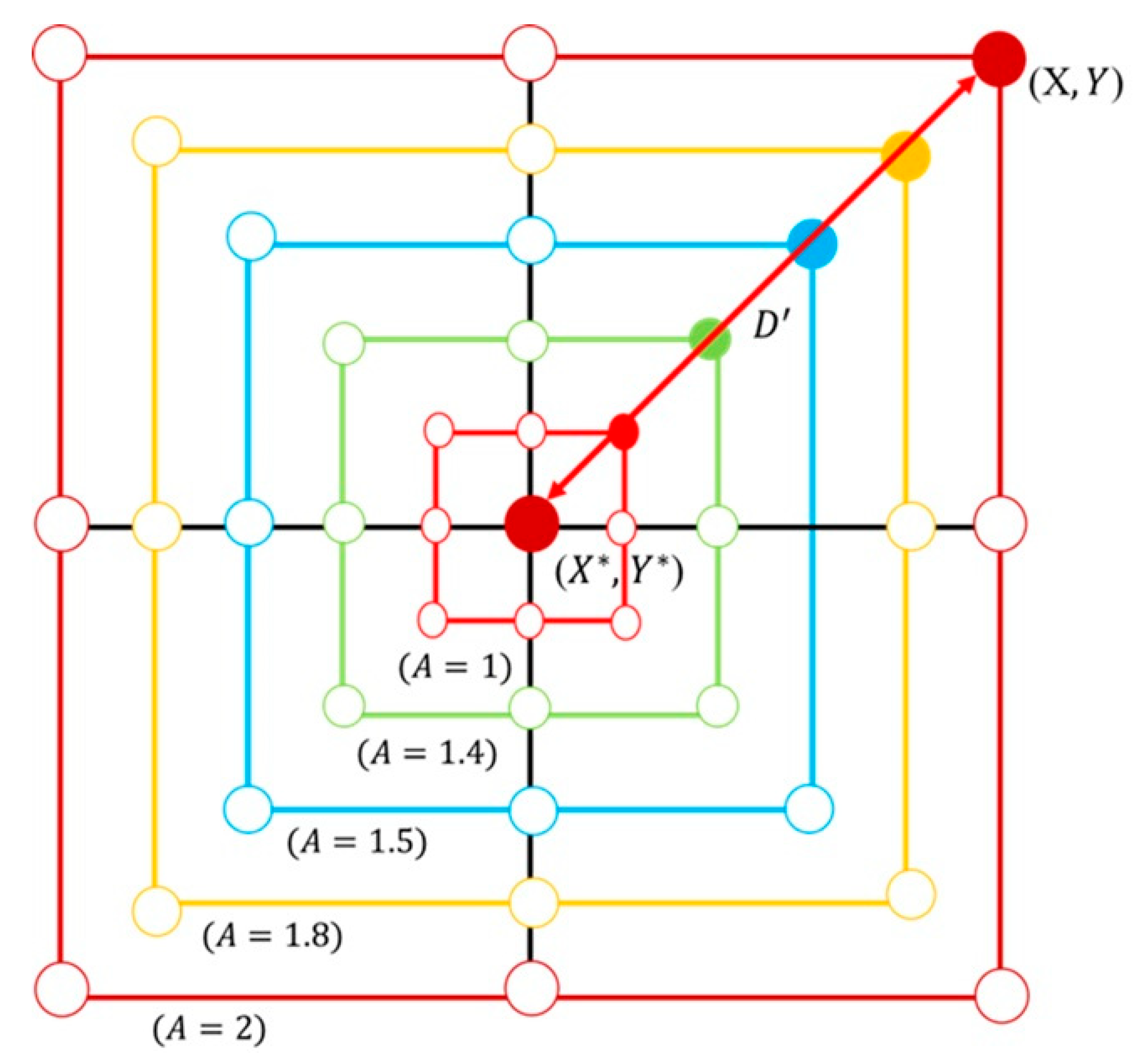
- 3. Bubble-net attacking method: There are two methods for modeling the whale's bubble-net feeding behavior: (1) the shrinking surround mechanism, and (2) the spiral position update [43]. As shown in Equation (20), this behavior is achieved by gradually decreasing the value of
. It is important to note that the range of also decreases along with a, where is a random value within the interval [−, ]. By setting as a random number between −1 and 1, the new position of a search agent can lie anywhere between its original location and the current best position. When , it illustrates all possible locations in 2D space between (X, Y) and (X* ,Y*), which essentially simulates the behavior of surround and hunting prey. Whales generate spiral-shaped bubble nets through their blowholes to trap prey, making it difficult for the prey to escape. They then move along this spiral bubble path to complete the hunt [44]. Based on the position of the best-identified prey, the whale generates a spiral bubble pattern and updates its position accordingly using Equation (22), as shown in Figure 10. The spiral position update is expressed by Equation (23):
Where is the spatial vector between the whale and the current best prey position; is a constant that defines the shape of the spiral bubble-net, and it is set to 1 in this study; is a random number between [−1, 1].
- 4. Search for prey: In addition to using the bubble-net method, whales also exhibit random prey-searching behavior during foraging, as illustrated in Figure 11. This behavior is based on a variable
vector, where whales perform random searches relative to each other’s positions. In this method, when is greater than 1 or less than -1, it drives the search to move away from the current location. Unlike the bubble-net method, this search mechanism does not rely on the best solution found so far, but rather updates positions based on randomly selected search agents [45]. This mechanism involves an vector magnitude greater than 1, as represented in Equations (24) and (25):
Where is the current random position of the whale population; is the position vector between the whale and a randomly selected prey.
- 5. Record the current highest profit until the search stopping condition is met: WOA continuously updates the optimal solution through iterative searching (i.e., minimizing the objective function defined in this study). Once the search stopping condition is met, the algorithm outputs the optimal solution; otherwise, it returns to steps (2), (3), and (4) to continue the computation until the stopping condition is satisfied or the computation is complete [46].
Figure 11.
Search diagram of the whale prey.
This study introduces two optimization methods for control strategies. Although the core computations differ in terms of the mathematical equations used during their respective search processes, both aim to optimize the same objective function, and the control variables used are identical to those in the GGS approach, as referenced in the GGS power distribution ratio formula. In the WOA, key control parameters typically include population size and the number of iterations. These parameters significantly affect the algorithm’s performance and convergence speed. In general, their values are adjusted according to the characteristics and requirements of the problem being addressed. In this study, vehicle energy efficiency simulations are conducted using MATLAB/Simulink®, with a sampling time of 0.01 s. The main focus is to compare the impact of different control strategies on vehicle energy efficiency rather than on the optimization of algorithm parameters themselves. Based on simulation results, using a larger population size yields better outcomes. The parameter settings are shown in Table 5.
In this study, the defined parameters are applied to the WOA for computation. The process begins with Step 1, which involves initializing the whale population, calculating fitness, updating whale positions, handling boundary conditions, and generating initial positions. In Step 2, the algorithm checks whether the maximum number of iterations has been reached. If not, it proceeds to Step 3, where a probability-based decision is made. Based on the value of , the algorithm selects a behavior mode: if 0.5, the spiral position update is performed; if 0.5, it proceeds to Step 4. In Step 4, the algorithm determines the step coefficient based on the relative distance between the whale and the prey using the value of . If 1, the whale performs a search for prey; if 1, the whale engages in shrinking surround behavior. Finally, the best solution is selected based on the optimal fitness value, and the process returns to Step 2 to continue the iterations until the stopping condition is met. The WOA flow is illustrated in Figure 12.
4. Simulation and Experimental Results
In this study, Matlab/Simulink® software is used to integrate the primary and secondary systems of a dual-motor electric vehicle. Both pure simulation and HIL simulation are employed to test the RBC, GGS, and WOA control methods for the entire vehicle system. The simulation results are then analyzed and discussed accordingly.
4.1. GGS Grid Point Testing
In this study, the resolution of the GGS method is constrained by grid spacing and hardware limitations. If the interval between parameter grid points is too large, the calculated conditions may not precisely align with the points on the multi-dimensional grid. In such cases, the system uses built-in interpolation methods to obtain a solution. Although this reduces computation time, the results may be suboptimal. Therefore, energy efficiency tests were conducted under the FTP-75 driving cycle using various GGS grid spacings to identify the most suitable grid design as a reference standard. As shown in Table 6, the average energy efficiency results over five FTP-75 simulations were recorded for grid spacings of 1, 0.5, 0.2, 0.1, 0.01, 0.005, and 0.001.
4.2. Parameter Adjustment Testing of Whale Optimization Algorithm
In this study, the parameters of the WOA were adjusted with respect to the count of iterations and the whale population size. Energy efficiency tests were conducted using the FTP-75 driving cycle, and the simulation results are presented in Table 7. It can be observed that the optimal (i.e., lowest) energy efficiency was achieved with 300 iterations and a whale population size of 50, as shown in Table 8. To explore the maximum simulation capacity of the hardware system, the iteration count was further increased from 300 to 400 to determine the highest number of iterations that can still be tested in real time.
4.3. Comparison of Vehicle Velocity Results
The FTP-75 driving cycle is mainly divided into two parts: the first part, from the start to the 505th second, is the cold-start phase, which primarily involves low- and medium- velocity driving patterns, including acceleration, cruising, and deceleration, with a maximum velocity of 91.25 km/h. The second part, from the 506th second to the 1370th second, is the hot-start phase, which features driving patterns similar to the cold-start phase, also including acceleration, cruising, and deceleration, with the same maximum velocity of 91.25 km/h. The energy management strategy determines the output torque of the dual power units based on the target vehicle velocity and the optimized power distribution ratio. To comprehensively verify whether the power distribution results of the energy management strategy can meet the required vehicle velocity, this study conducted both a single-cycle and five-cycle FTP-75 test. Figure 13 and Figure 14 show the vehicle velocity tracking and velocity error results for a single FTP-75 cycle. As observed from the two graphs, the dual power units provide sufficient power to reach the target velocity, with the velocity error controlled within ±1 km/h. However, according to Figure 15 and Figure 16, which present the vehicle velocity tracking and velocity error results over five FTP-75 cycles, it can be seen that under the RBC, GGS, and WOA control strategies, the dual-motor system is capable of delivering sufficient power to achieve the target velocity, with velocity errors maintained within ±2 km/h.
4.4. Torque Output Results under the Different Control Strategies
The energy management strategy proposed in this study aims to achieve higher energy efficiency and improved computational efficiency by applying three control strategies to regulate the power output of the front and rear axle motors. Figure 17 illustrates the torque outputs of the front and rear axle motors during a single execution of the FTP-75 driving cycle, whereas Figure 18 presents these results over five consecutive FTP-75 driving cycles. According to the RBC strategy shown in Figure 17 and implemented based on the control logic defined in Table 3, the power distribution during a single FTP-75 driving cycle operates as follows: during vehicle acceleration, the front and rear axis motors output torque in a 30 % to 70 % distribution ratio. When the vehicle velocity exceeds 50 km/h, the demanded torque is primarily handled by the rear axis motor. Under the GGS and WOA control strategies, the initial acceleration demanded torque is mainly provided by the front motor. However, during mid-range acceleration, the front motor ceases power output, and once the velocity exceeds 50 km/h, the rear axis motor becomes the primary source of torque.
As shown in Figure 18, the five-cycle driving behavior closely follows the same trend observed in the single-cycle scenario. All three control strategies are capable of meeting the intended control design requirements.
4.5. HIL output results under the Different Control Strategies
To validate the effectiveness of the proposed control strategies, this study employed HIL testing to verify the consistency between dual-power model outputs and WOA computer simulation results. Figure 19 presents the motor torque output results from a single execution of each strategy for the front and rear axle motors, while Figure 20 shows motor torque output results from five executions of each control strategy. As observed in Figure 19, under the RBC strategy, the torque output frequency of the front axle motor is relatively low and concentrated primarily during specific acceleration phases. In contrast, the rear axle motor consistently outputs torque throughout most of the operation, indicating that the rear motor primarily drives the vehicle. Examining the torque output results for GGS and WOA strategies, the front axle motor exhibits regular torque outputs during vehicle acceleration phases, demonstrating more synchronized output behavior between the front and rear axle motors under high torque conditions. According to Figure 20, the torque outputs from the front and rear axle motors for both computer simulations and HIL tests demonstrate a certain degree of similarity. The high frequency of front and rear axle coordination across all three control strategies ensures effective utilization. However, discrepancies are apparent in the HIL environment due to constraints such as noise and system overheating. While similarities remain evident between simulation and HIL torque outputs, noticeable oscillations exist, likely caused by signal scaling, which introduces differences between transmitted and original signals, thereby generating errors.
4.6. Torque Output Results under the Different Control Strategies
The energy efficiency of the entire vehicle, simulated under various control strategies, serves as a benchmark for comparison. The detailed results are shown in Table 8 and Table 9. These tables respectively present the energy efficiency outcomes under three different control strategies (RBC, GGS, and WOA) comparing both pure simulation and HIL scenarios. According to the data analysis from Table 9 and Table 10, it is evident that both the GGS and WOA control strategies significantly improve energy efficiency. Specifically, the GGS strategy demonstrates slightly better energy performance than the WOA strategy. However, the WOA strategy still exhibits outstanding performance, with results closely aligning with those of GGS. Compared to the RBC strategy, the GGS and WOA strategies improve energy efficiency by 9.1 % and 8.9 %, respectively. Further analysis of the HIL testing results shows that the WOA-based energy management strategy performs not only well in computer simulations but also demonstrates high feasibility in real-world hardware environments. The HIL test results indicate that, compared to the RBC strategy, the GGS and WOA strategies improve energy efficiency by 4.2 % and 3.8 %, respectively. Although the GGS strategy achieves slightly better energy efficiency, the WOA strategy proves to be a highly promising alternative for practical implementation of efficient energy distribution.
5. Conclusions
This study established a simulation platform using Matlab/Simulink® to model a real-world Tesla Model X vehicle equipped with front and rear axle motor systems. The specifications and characteristic curves of each power source system were developed, and the following conclusions were drawn:
- Ø Dual-Motor Electric Vehicle Model Development: A physics-based control model was developed using existing Tesla Model X vehicle parameters. Speed-tracking simulations were performed under various control strategies. The constructed model comprises sub-models for the driving cycle, driver behavior, electric motor dynamics, lithium battery characteristics, vehicle dynamics, and the energy management system, ensuring reliable and stable operation of the front and rear axle motor systems in practical applications.
- Ø Application of Energy Control Strategies: Based on the dual-motor system simulation platform developed in Matlab/Simulink®, the study implemented and tested three different control strategies: RBC, GGS and WOA.
- Ø Validation via Pure Simulation and HIL Simulation: A closed-loop real-time simulation platform was established using an Arduino DUE microcontroller and a TI C2000 microcontroller in series. This platform was used to verify the WOA-based energy management system. Real-time computation was carried out in a HIL environment, and the results were compared with those from the pure simulation to assess consistency.
- Ø Validation Under FTP-75 Driving Cycle:
- Ø Pure Simulation: Compared with the RBC, GGS and WOA control strategies improved energy efficiency by 9.1 % and 8.9 %, respectively.
- Ø HIL Simulation: Under HIL conditions, energy efficiency improvements of 4.2 % and 3.8 % were achieved using GGS and WOA, respectively, compared to the RBC.
Author Contributions
Conceptualization, C.-H.W. and C.-L.T.; Methodology, C.-H.W.; Software, C.-L.T. and J.-M.Y.; Validation, C.-L.T. and J.-M.Y.; Formal Analysis, C.-H.W. and C.-L.T.; Investigation, C.-H.W.; Data Curation, C.-L.T. and J.-M.Y.; Writing-Original Draft, C.-H.W.; Writing-Review & Editing, C.-H.W.; Visualization, C.-H.W.; Resources, C.-H.W.; Supervision, C.-H.W.; Project Administration, C.-H.W.; Funding Acquisition, C.-H.W.
Funding
The authors would like to thank the National Science and Technology Council of the Republic of China, Taiwan, for financial support for this research under Contract No. NSTC 111-2221-E-027-081-MY3; and thanks to the APh ePower Co., Ltd. project for advanced vehicle control.
Conflicts of Interest
The authors declare no conflict of interest.
Nomenclature
| power distribution ratio of the first gear | |
| represents the relationship between battery | |
| rolling resistance coefficient | |
| air density | |
| efficiency of the battery charge and discharge | |
| overall efficiency of the final drive | |
| efficiency of the drive motor | |
| efficiency of the front axis motor | |
| efficiency of the rear axis motor | |
| the step coefficient | |
| frontal area of the EV | |
| decreases linearly from 2 to 0 during the iteration process | |
| a constant that defines the shape of the spiral bubble-net | |
| the weighting coefficient | |
| drag coefficient | |
| the position vector between the whale and a randomly selected prey | |
| the spatial vector between the whale and the current best prey position | |
| input power of the front axis motor | |
| input power of the rear axis motor | |
| braking force | |
| gravitational acceleration | |
| charge and discharge current of the battery | |
| optimal objective function | |
| a random number between [−1, 1] | |
| integral gain of the PI controller | |
| proportional gain of the PI controller | |
| the lower bound of the control variable being searched | |
| total vehicle mass | |
| wheel speed of the drive motor | |
| maximum number of iterations | |
| the maximum number of iterations | |
| the current iteration number | |
| probability | |
| discharge power of the battery | |
| rated capacity of the lithium battery | |
| equivalent internal resistance of the lithium battery gradient resistance | |
| wheel radius | |
| the random vector within the range [0, 1] | |
| state of charge for lithium battery | |
| state of charge initial value of lithium battery | |
| total demand torque | |
| the output torque of the final drive | |
| output torque of the drive motor | |
| output torque of the front axis motor | |
| output torque of the rear axis motor | |
| time or current number of iterations | |
| the temperature of the battery | |
| the upper bound of the control variable being searched | |
| the dimensional size of the control variable | |
| voltage of the lithium battery | |
| vehicle velocity | |
| open circuit voltage of the lithium battery | |
| the error between the demand vehicle velocity and the actual vehicle velocity | |
| population size of whale | |
| the current position | |
| the position of the current best solution | |
| the current random position of the whale population | |
References
- Meng, Y.B.; Kong, H.F.; Liu, T.K. Multi-Source Information Fusion for Environmental Perception of Intelligent Vehicles Using Sage-Husa Adaptive Extended Kalman Filtering. Sensors 2025, 25, 198. [Google Scholar] [CrossRef] [PubMed]
- Qarout, Y.; Raykov, Y.P.; Little, M.A. Probabilistic Modelling for Unsupervised Analysis of Human Behaviour in Smart Cities. Sensors 2020, 20, 784. [Google Scholar] [CrossRef]
- Li, F.X.; Wang, X.L.; Bao, X.C.; Wang, Z.Y.; Li, R.X. Energy Management Strategy for Fuel Cell Vehicles Based on Online Driving Condition Recognition Using Dual-Model Predictive Control. Sensors 2024, 24, 7647. [Google Scholar] [CrossRef]
- Pang, Q.H.; Qiu, M.; Zhang, L.; Chiu, Y.H. Congestion effects of Energy and its Influencing Factors: China's Transportation Sector. Socio-Economic Planning Sciences 2024, 92, 101850. [Google Scholar] [CrossRef]
- Nunes, L.J.R. The Rising Threat of Atmospheric CO2: A Review on the Causes, Impacts, and Mitigation Strategies. Environments 2023, 10, 66. [Google Scholar] [CrossRef]
- Thomas, F.; Livio, F.A.; Ferrario, F.; Pizza, M.; Chalaturnyk, R. A Review of Subsidence Monitoring Techniques in Offshore Environments. Sensors 2024, 24, 4164. [Google Scholar] [CrossRef]
- Wang, J.W.; Topilin, I.; Feofilova, A.; Shao, M.; Wang, Y.D. Cooperative Intelligent Transport Systems: The Impact of C-V2X Communication Technologies on Road Safety and Traffic Efficiency. Sensors 2025, 25, 2132. [Google Scholar] [CrossRef]
- Elsheikh, A.; Ali, A.B.M.; Saba, A.; Faqeha, H.; Alsaati, A.A.; Maghfuri, A.M.; Abd-Elaziem, W.; Ashmawy, A.A.E.; Ma, N.S. A Review on Sustainable Machining: Technological Advancements, Health and Safety Considerations, and Related Environmental Impacts. Results in Engineering 2024, 24, 103042. [Google Scholar] [CrossRef]
- Yang, K.X.; Zhang, Q.; Liu, Q.Q.; Liu, J.F.; Jiao, J. Effect Mechanism and Efficiency Evaluation of Financial Support on Technological Innovation in the New Energy Vehicles’ Industrial Chain. Energy 2024, 293, 130761. [Google Scholar] [CrossRef]
- Wójcik, G.; Przystałka, P. Towards Safer Electric Vehicles: Autoencoder-Based Fault Detection Method for High-Voltage Lithium-Ion Battery Packs. Sensors 2025, 25, 1369. [Google Scholar] [CrossRef]
- Oubelaid, A.; Taib, N.; Rekioua, T.; Bajaj, M.; Blazek, V.; Prokop, L.; Misak, S.; Ghoneim, S.S.M. Multi Source Electric Vehicles: Smooth Transition Algorithm for Transient Ripple Minimization. Sensors 2022, 22, 6772. [Google Scholar] [CrossRef] [PubMed]
- Kwon, H.J.; Choi, Y.G.; Choi, W.S.; Lee, S.W. Multimode Dual-motor Electric Vehicle System for Eco and Dynamic Driving. Results in Engineering 2023, 19, 101298. [Google Scholar] [CrossRef]
- Rani, S.; Jayapragash, R. Review on Electric Mobility: Trends, Challenges and Opportunities. Results in Engineering 2024, 23, 102631. [Google Scholar]
- Wang, D.; Mei, L.; Xiao, F.; Song, C.X.; Qi, C.Y.; Song, S.X. Energy Management Strategy for Fuel Cell Electric Vehicles Based on Scalable Reinforcement Learning in Novel Environment. International Journal of Hydrogen Energy 2024, 59, 668–678. [Google Scholar] [CrossRef]
- Tariq, A.H.; Anwar, M.; Kazmi, S.A.A.; Hassan, M.; Bahadar, A. Techno-economic and Composite Performance Assessment of Fuel Cell-based Hybrid Energy Systems for Green Hydrogen Production and Heat Recovery. International Journal of Hydrogen Energy 2025, 104, 444–462. [Google Scholar] [CrossRef]
- Takrouri, M.A.; Idris. N.R.N.; Aziz, M.J.A.; Ayop, R.; Low, W.Y. Refined Power Follower Strategy for Enhancing the Performance of Hybrid Energy Storage Systems in Electric Vehicles. Results in Engineering 2025, 25, 103960. [Google Scholar] [CrossRef]
- Wang, Z.; Zhou, J.; Rizzoni, G. A Review of Architectures and Control Strategies of Dual-motor Coupling Powertrain Systems for Battery Electric Vehicles. Renewable and Sustainable Energy Reviews 2022, 162, 112455. [Google Scholar] [CrossRef]
- Zhai, L.; Zhang, X.Y.; Wang, Z.D.; Mok, Y.M.; Hou, R.F.; Hou, Y.H. Steering Stability Control for Four-Motor Distributed Drive High-Speed Tracked Vehicles. IEEE Access 2020, 8, 94968–94983. [Google Scholar] [CrossRef]
- Khadatkar, A.; Sujit, P.B.; Agarwal, R.; Viswanath, K.; Sawant, C.P.; Magar, A.P.; Chaudhary, V.P. WeeRo: Design, Development and Application of a Remotely Controlled Robotic Weeder for Mechanical Weeding in Row Crops for Sustainable Crop Production. Results in Engineering 2025, 26, 105202. [Google Scholar] [CrossRef]
- Tian, Y.; Wang, Z.H.; Ji, X.Y.; Ma, L.; Zhang, L.P.; Hong, X.Q.; Zhang, N. A Concept Dual-motor Powertrain for Battery Electric Vehicles: Principle, Modeling and Mode-shift. Mechanism and Machine Theory 2023, 185, 105330. [Google Scholar] [CrossRef]
- Zhang, F.Q.; Wang, L.H.; Coskun, S.; Pang, H.; Cui, Y.H.; Xi, J.Q. Energy Management Strategies for Hybrid Electric Vehicles: Review, Classification, Comparison, and Outlook. Energies 2020, 13, 3352. [Google Scholar] [CrossRef]
- Xu, Y.H.; Zhang, H.G.; Yang, Y.F.; Zhang, J.; Yang, F.B.; Yan, D.; Yang, H.L.; Wang, Y. Optimization of Energy Management Strategy for Extended Range Electric Vehicles Using Multi-island Genetic Algorithm. Journal of Energy Storage 2023, 61, 106802. [Google Scholar] [CrossRef]
- Oliveira Farias, H.E.; Sepulveda Rangel, C.A.; Weber Stringini, L.; Neves Canha, L.; Pegoraro Bertineti, D.; da Silva Brignol, W.; Iensen Nadal, Z. Combined Framework with Heuristic Programming and Rule-Based Strategies for Scheduling and Real Time Operation in Electric Vehicle Charging Stations. Energies 2021, 14, 1370. [Google Scholar] [CrossRef]
- Ullah, K.; Ishaq, M.; Tchier, F.; Ahmad, H.; Ahmad, Z. Fuzzy-based Maximum Power Point Tracking (MPPT) Control System for Photovoltaic Power Generation System. Results in Engineering 2023, 20, 101466. [Google Scholar] [CrossRef]
- Yang, C.; Du, S.Y.; Li, L.; You, S.X.; Yang, Y.Y.; Zhao, Y. Adaptive Real-time Optimal Energy Management Strategy Based on Equivalent Factors Optimization for Plug-in Hybrid Electric Vehicle. Applied Energy 2017, 203, 883–896. [Google Scholar] [CrossRef]
- Mao, T.; Zhang, X.; Zhou, B.R. Intelligent Energy Management Algorithms for EV-charging Scheduling with Consideration of Multiple EV Charging Modes. Energies 2019, 12, 265. [Google Scholar] [CrossRef]
- Korkas, C.D.; Terzopoulos, M.; Tsaknakis, C.; Kosmatopoulos, E.B. Nearly Optimal Demand Side Management for Energy, Thermal, EV and Storage Loads: An Approximate Dynamic Programming Approach for Smarter Buildings. Energy and Buildings 2022, 255, 111676. [Google Scholar] [CrossRef]
- Abdullah-Al-Nahid. S.; Khan. T.A.; Taseen. M.A.; Jamal. T.; Aziz. T. A Novel Consumer-friendly Electric Vehicle Charging Scheme with Vehicle to Grid Provision Supported by Genetic Algorithm Based Optimization. Journal of Energy Storage 2022, 50, 104655. [Google Scholar] [CrossRef]
- Cheng, J.C.; Xu, J.D.; Chen, W.T.; Song, B.B. Locating and Sizing Method of Electric Vehicle Charging Station Based on Improved Whale Optimization Algorithm. Energy Reports 2022, 8, 4386–4400. [Google Scholar] [CrossRef]
- Saha. N.; Mishra. P.C. Modified Whale Algorithm-Based Optimization for Fractional Order Concurrent Diminution of Torque Ripple in Switch Reluctance Motor for EV Applications. Processes 2023, 11, 1226. [Google Scholar] [CrossRef]
- Tesla Model X. (2025). [Online]. Available online: https://www.tesla.com/ownersmanual/modelx/en_us/ (accessed on 3 June 2025).
- ZEPT EDM-S (2025). [Online]. 3 June. Available online: https://www.zept.com.tw/edm1-s-p95 (accessed on 3 June 2025).
- Baek, S.H.; Cho, J.H.; Kim, K.J.; Ahn, S.H.; Myung, C.L.; Park, S.S. Effect of the Metal-Foam Gasoline Particulate Filter (GPF) on the Vehicle Performance in a Turbocharged Gasoline Direct Injection Vehicle over FTP-75. International Journal of Automotive Technology 2020, 21, 1139–1147. [Google Scholar] [CrossRef]
- Zheng, W.J.; Luo. Y.; Pi. Y.G.; Chen. Y.Q. Improved Frequency-domain Design Method for the Fractional Order Proportional–integral–derivative Controller Optimal Design: a Case Study of Permanent Magnet Synchronous Motor speed Control. IET Control Theory & Applications 2018, 12, 2478–2487. [Google Scholar]
- Uralde, J.; Barambones, O.; Artetxe, E.; Calvo, I.; del Rio, A. Model Predictive Control Design and Hardware in the Loop Validation for an Electric Vehicle Powertrain Based on Induction Motors. Electronics 2023, 12, 4516. [Google Scholar] [CrossRef]
- Gong, W.M.; Liu, C.; Zhao, X.B.; Xu, S.K. A Model Review for Controller-hardware-in-the-loop Simulation in EV Powertrain Application. IEEE Transactions on Transportation Electrification 2024, 10, 925–937. [Google Scholar] [CrossRef]
- Cha, M.; Enshaei, H.; Nguyen, H.; Jayasinghe, S.G. Towards a Future Electric Ferry Using Optimisation-based Power Management Strategy in Fuel Cell and Battery Vehicle Application — A Review. Renewable and Sustainable Energy Reviews 2023, 183, 113470. [Google Scholar] [CrossRef]
- Louback, E.; Biswas, A.; Machado, F.; Emadi, A. A Review of the Design Process of Energy Management Systems for Dual-motor Battery Electric Vehicles. Renewable and Sustainable Energy Reviews 2024, 193, 114293. [Google Scholar] [CrossRef]
- Sahwal, C.P.; Sengupta, S.; Dinh, T.Q. Advanced Equivalent Consumption Minimization Strategy for Fuel Cell Hybrid Electric Vehicles. Journal of Cleaner Production 2024, 437, 140366. [Google Scholar] [CrossRef]
- Mirjalili, S.; Lewis, A. The Whale Optimization Algorithm. Advances in Engineering Software 2016, 95, 51–67. [Google Scholar] [CrossRef]
- Zhang, H.; Tang, L.; Yang, C.; Lan, S.L. Locating Electric Vehicle Charging Stations with Service Capacity Using the Improved Whale Optimization Algorithm. Advanced Engineering Informatics 2019, 41, 100901. [Google Scholar] [CrossRef]
- Li, Y.; Pei, W.; Zhang, Q. Improved Whale Optimization Algorithm Based on Hybrid Strategy and Its Application in Location Selection for Electric Vehicle Charging Stations. Energies 2022, 15, 7035. [Google Scholar] [CrossRef]
- Shaheen, H.I.; Rashed, G.I.; Yang, B.; Yang, J. Optimal Electric Vehicle Charging and Discharging Scheduling Using Metaheuristic Algorithms: V2G Approach for Cost Reduction and Grid Support. Journal of Energy Storage 2024; 90, 111816. [CrossRef]
- Adil, H.M.M.; Khan, H.A. WOA-tuned Supertwisted Synergetic Control of Multipurpose On-board Charger for G2V/V2G/V2V Operational Modes of Electric Vehicles. Control Engineering Practice 2025, 154, 106136. [Google Scholar] [CrossRef]
- Siahroodi, H.J.; Mojallali, H.; Mohtavipour, S.S. A Novel Multi-objective Framework for Harmonic Power Market Including Plug-in Electric Vehicles as Harmonic Compensators Using a New Hybrid Gray Wolf-whale-differential Evolution Optimization. Journal of Energy Storage 2022, 52, 105011. [Google Scholar] [CrossRef]
- Tang, M.N.; Jiang, Y.D.; Yu, S.Y.; Qiu, J.D.; Li, H.T.; Sheng, W.X. Non-dominated Sorting WOA Electric Vehicle Charging Station Siting Study Based on Dynamic Trip Chain. Electric Power Systems Research 2025, 244, 111532. [Google Scholar] [CrossRef]
Figure 1.
System architecture of the dual-motor drive system.
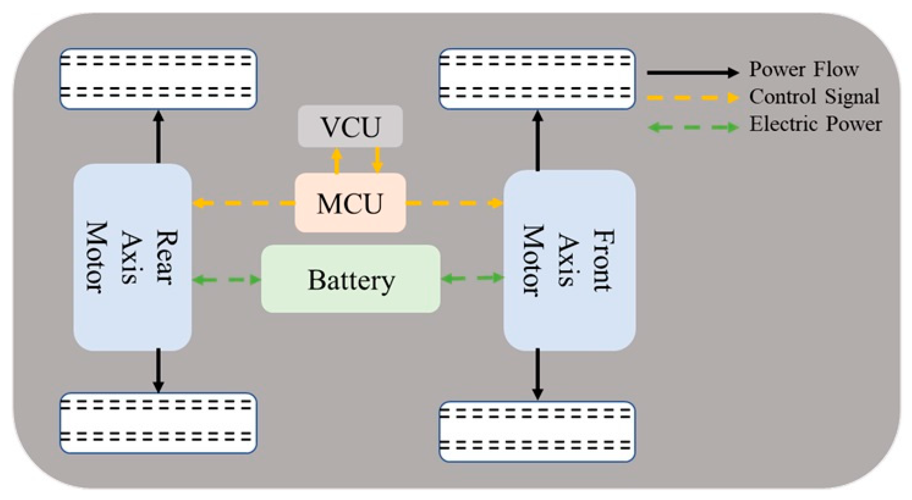
Figure 2.
Schematic diagram of the vehicle simulation platform software.
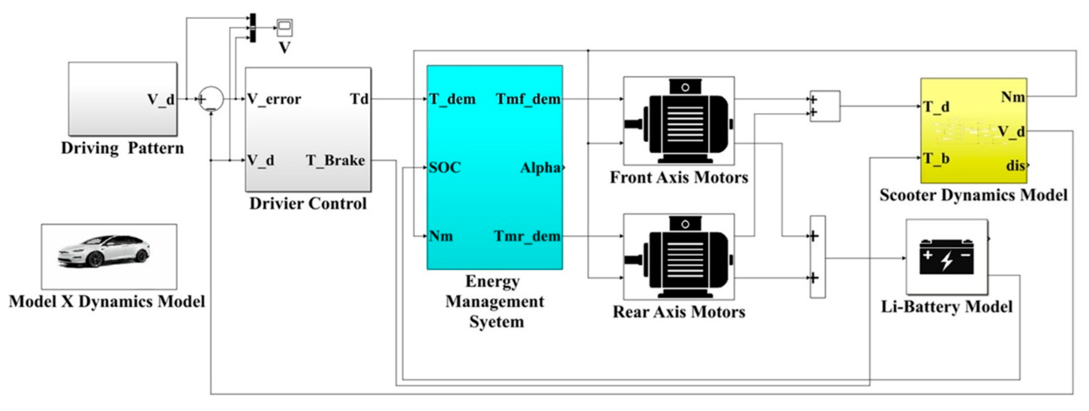
Figure 3.
FTP-75 driving cycle.
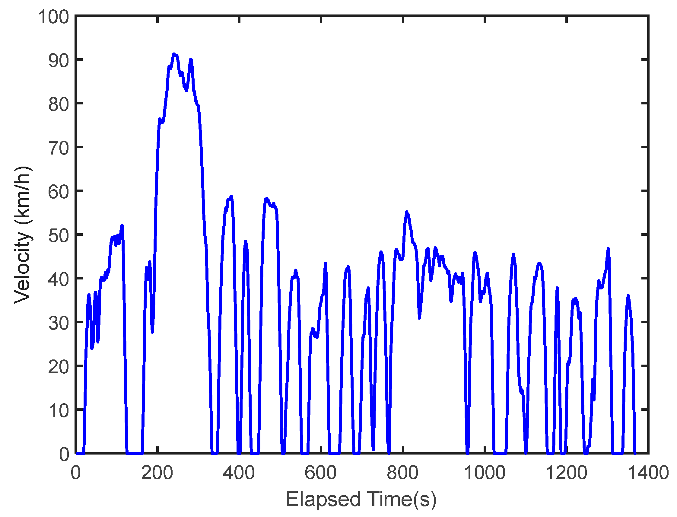
Figure 4.
Efficiency curve of the drive motor.
Figure 5.
Real-time model software of the VCU.
Figure 6.
Real-time model software of the vehicle platform.
Figure 7.
System architecture of the HIL using the Arduino DUE and Ti C2000.
Figure 8.
Control architecture of the energy management system.
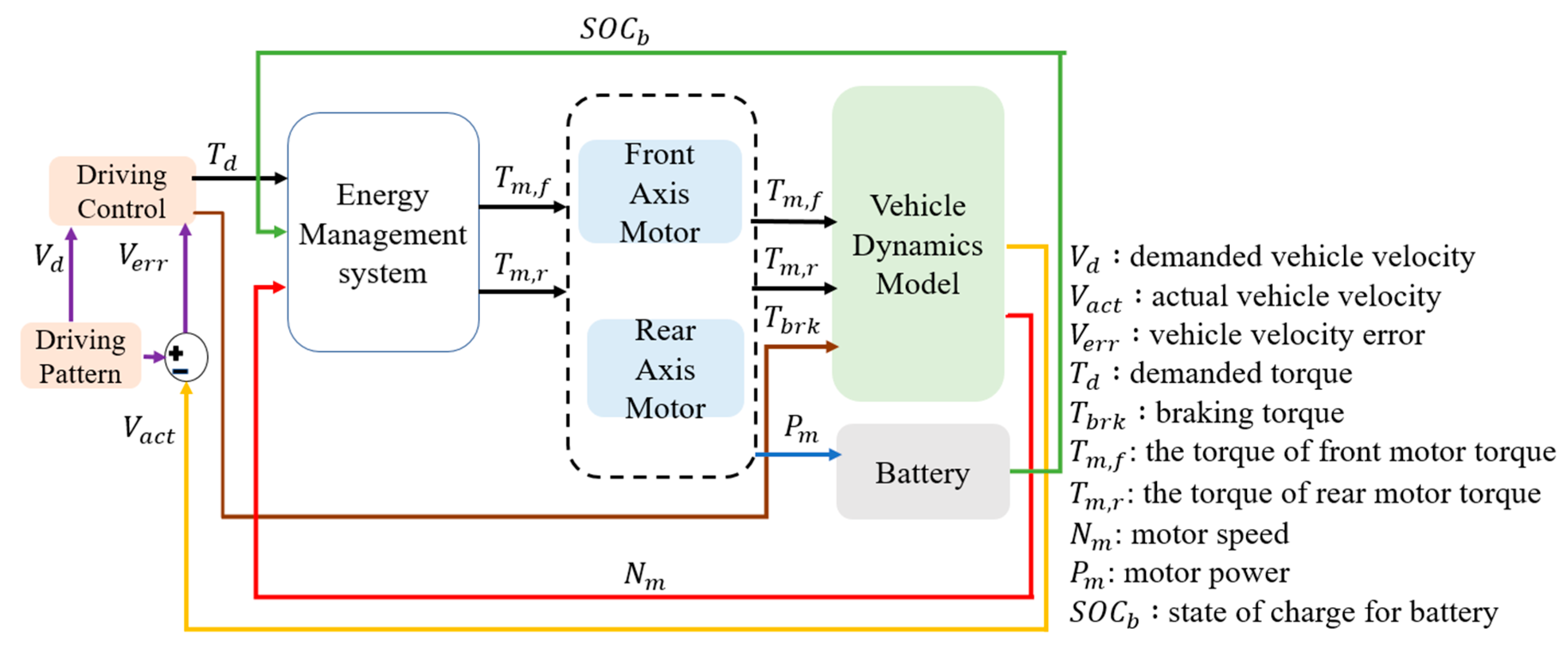
Figure 9.
Optimal power distribution loop for the front and rear axis motors.
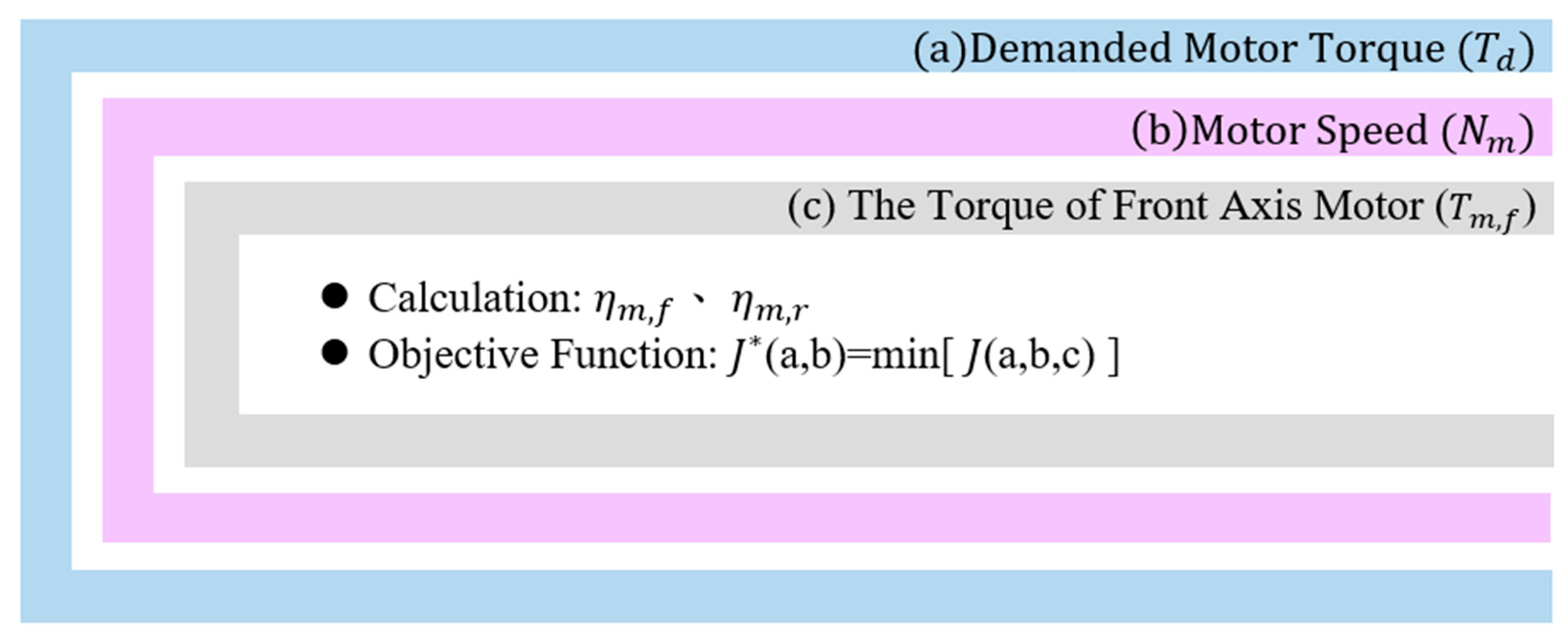
Figure 10.
Update diagram of the spiral position.
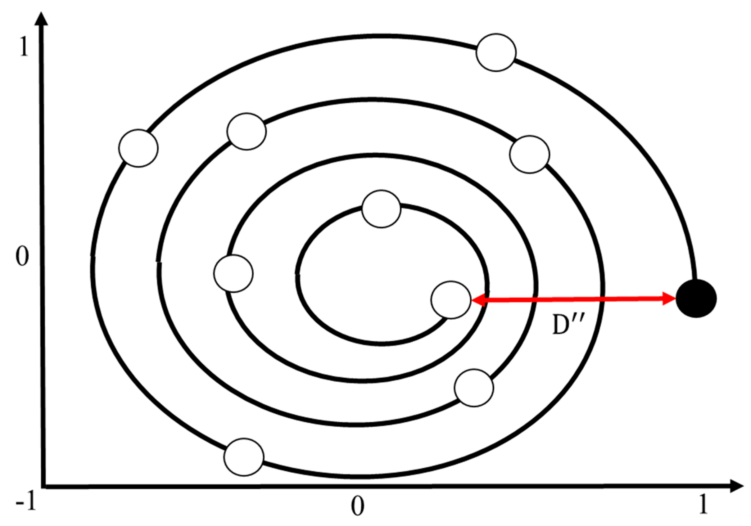
Figure 12.
Flowchart of the WOA.
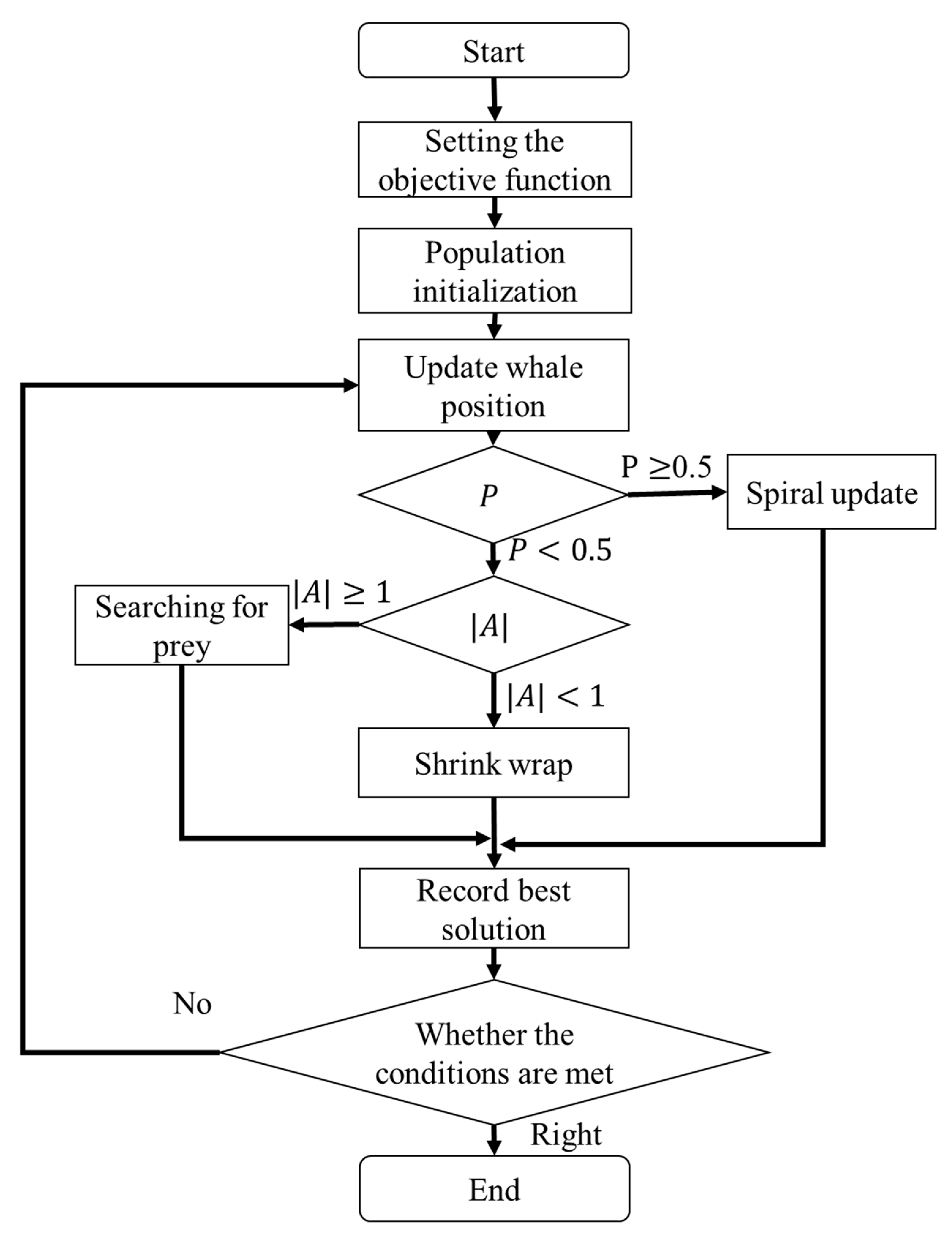
Figure 13.
Vehicle velocity for single FTP-75 driving cycle.
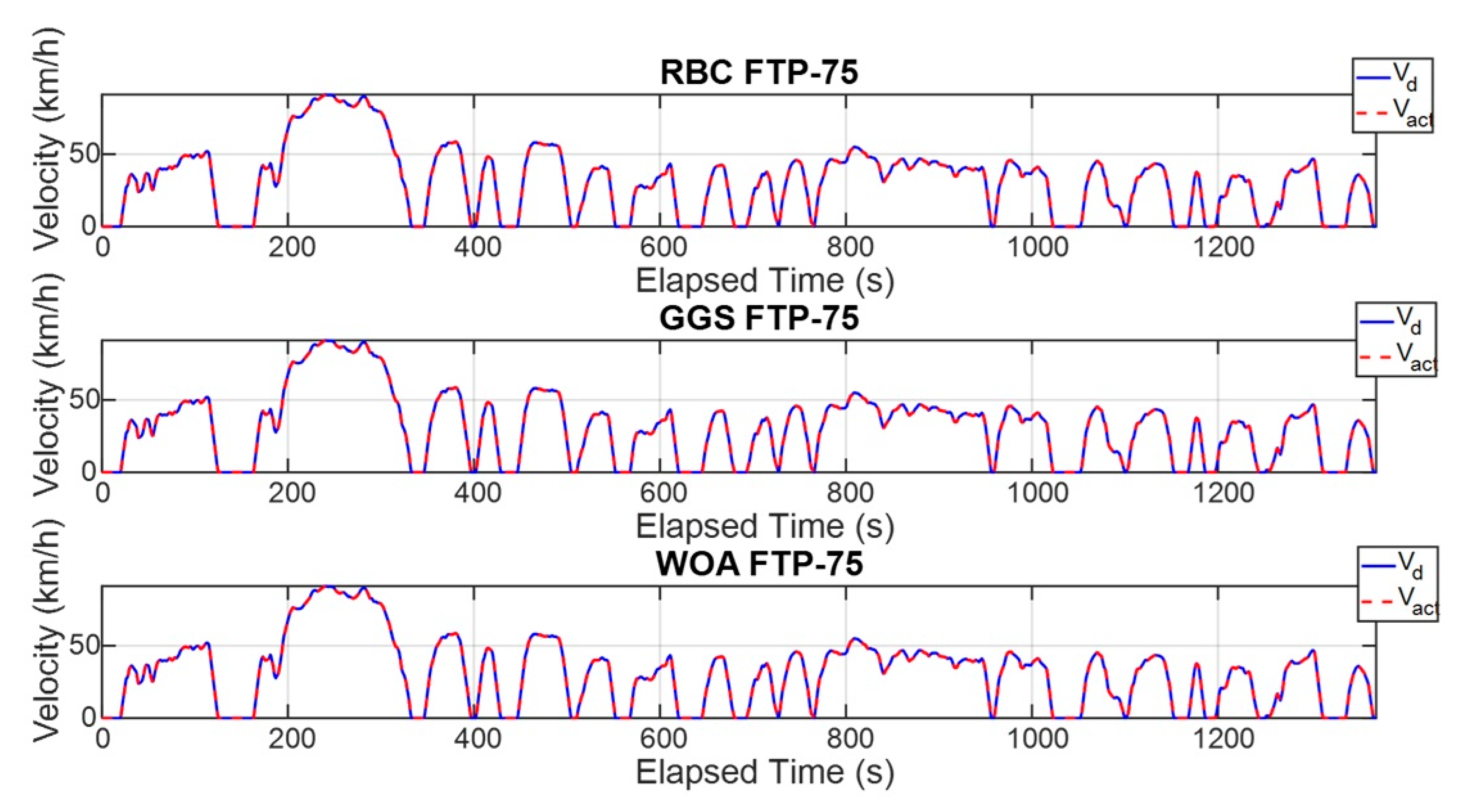
Figure 14.
Vehicle velocity error for single FTP-75 driving cycle.
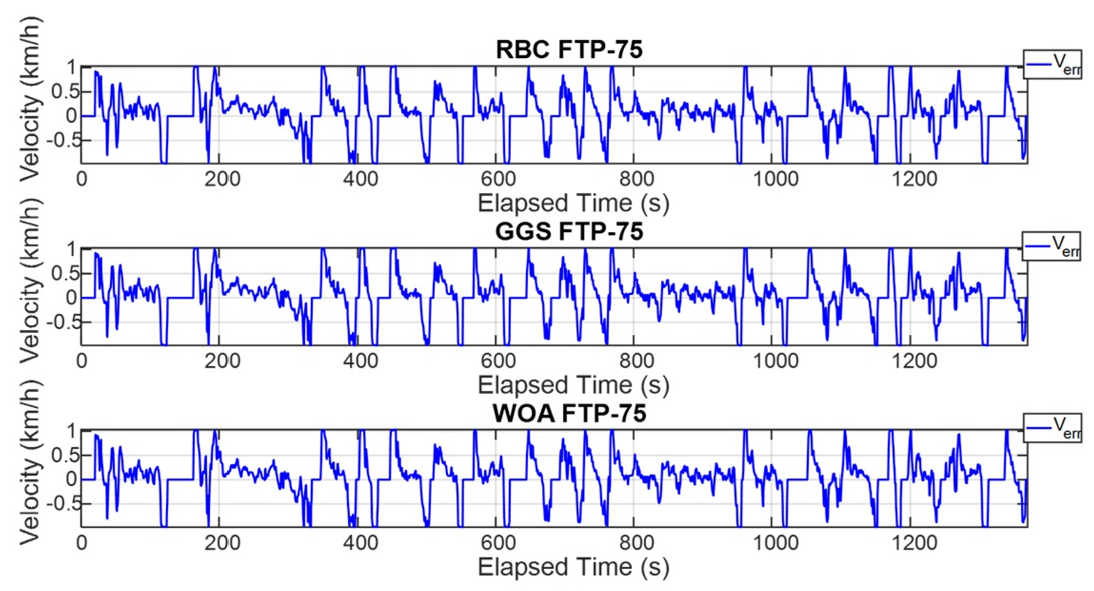
Figure 15.
Vehicle velocity for five FTP-75 driving cycle.
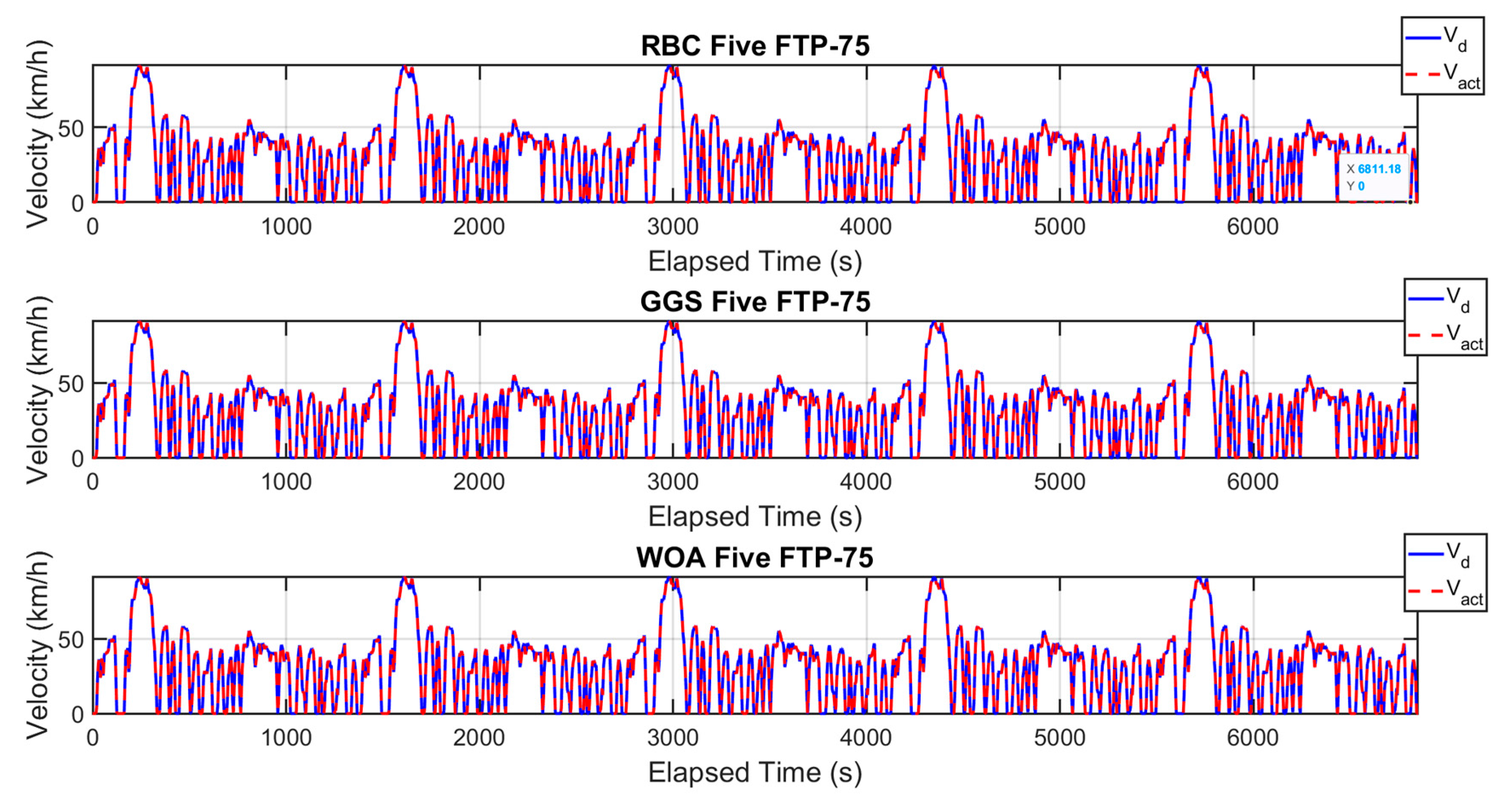
Figure 16.
Vehicle velocity error for five FTP-75 driving cycle.
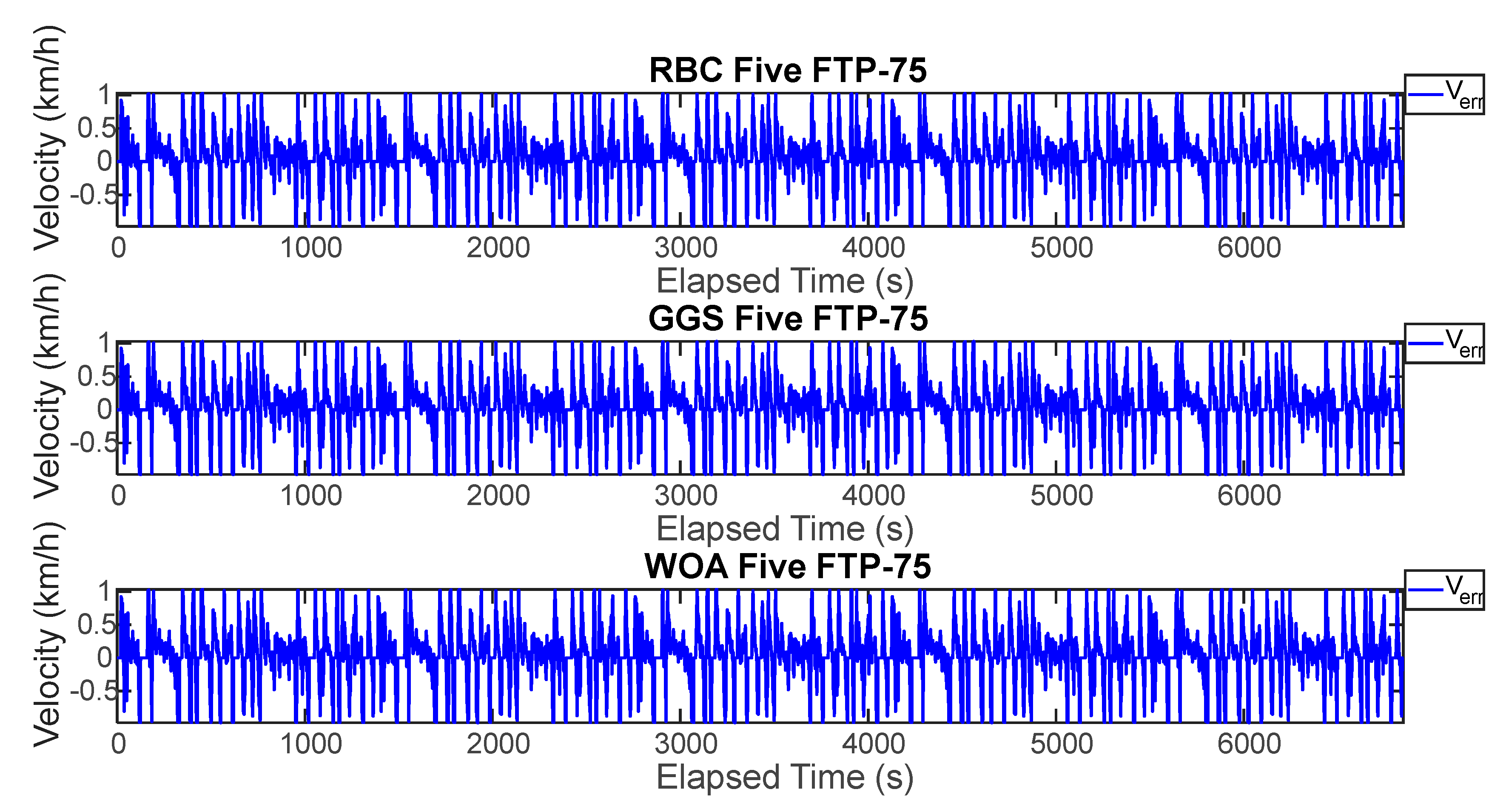
Figure 17.
Torque output of the front and rear axis motor for single FTP-75 driving cycle.
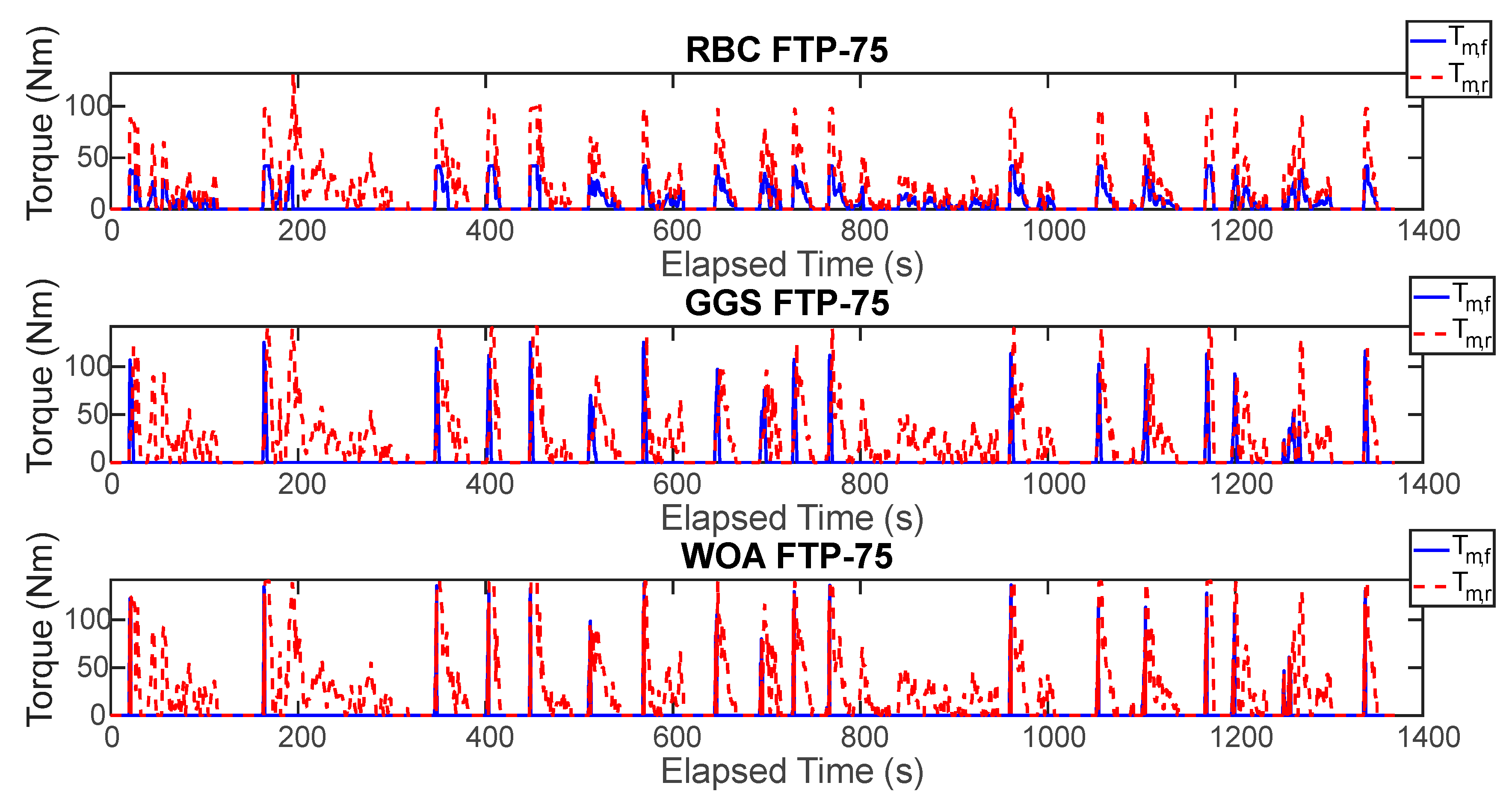
Figure 18.
Torque output of the front and rear axis motor for five FTP-75 driving cycle.
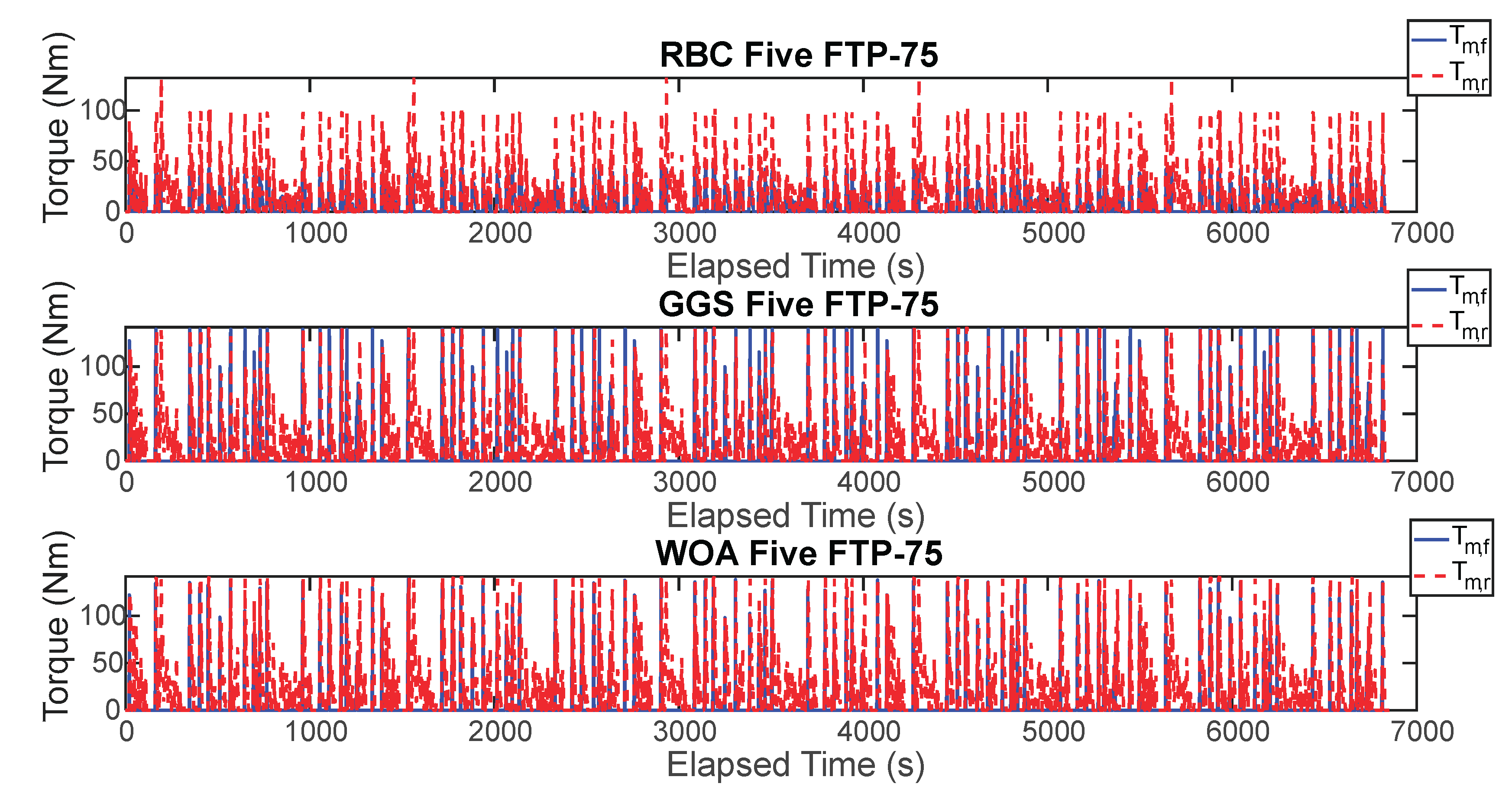
Figure 19.
HIL output results under different control strategies for single FTP-75 driving cycle.
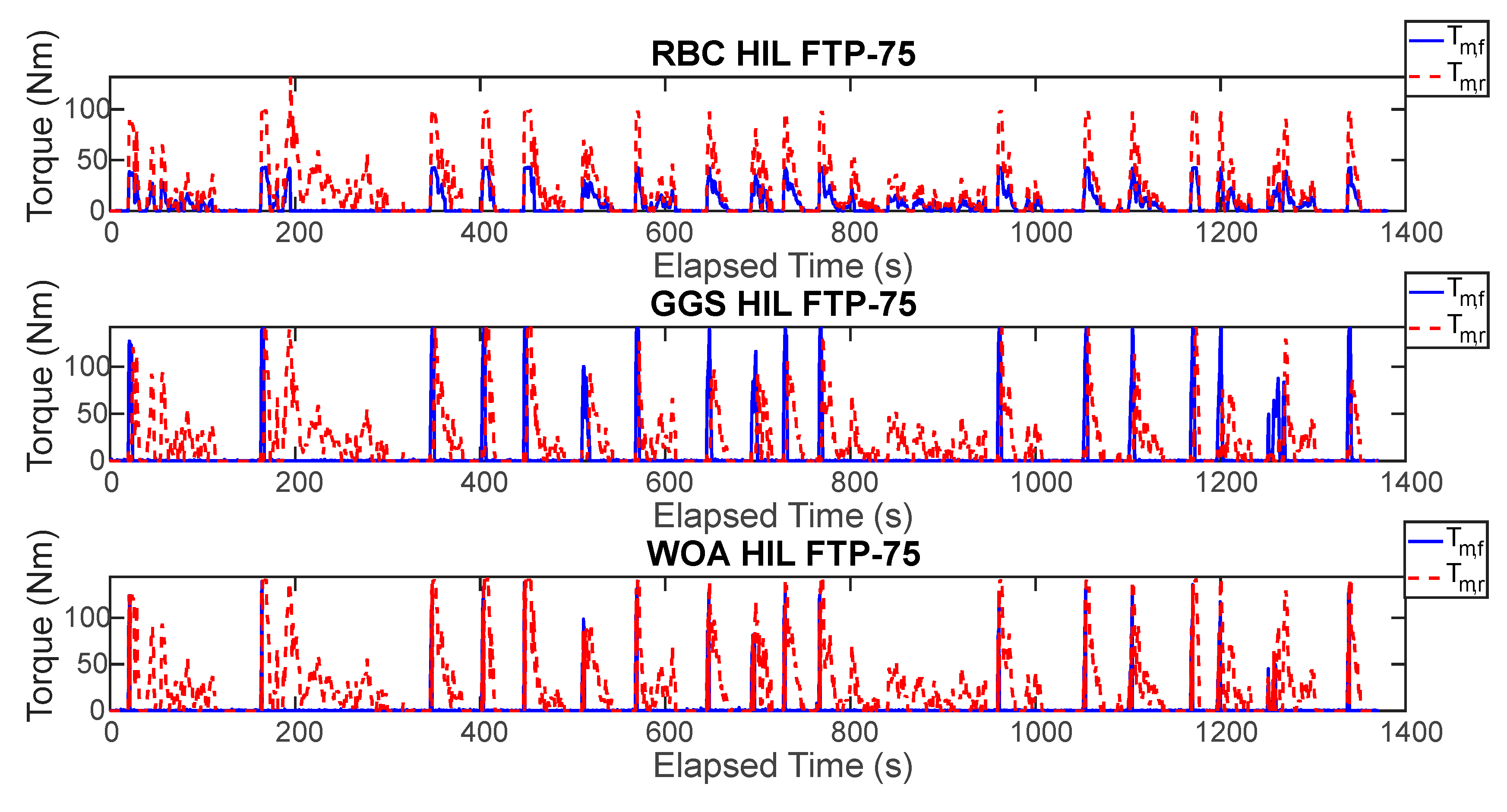
Figure 20.
HIL output results under different control strategies for five FTP-75 driving cycle.
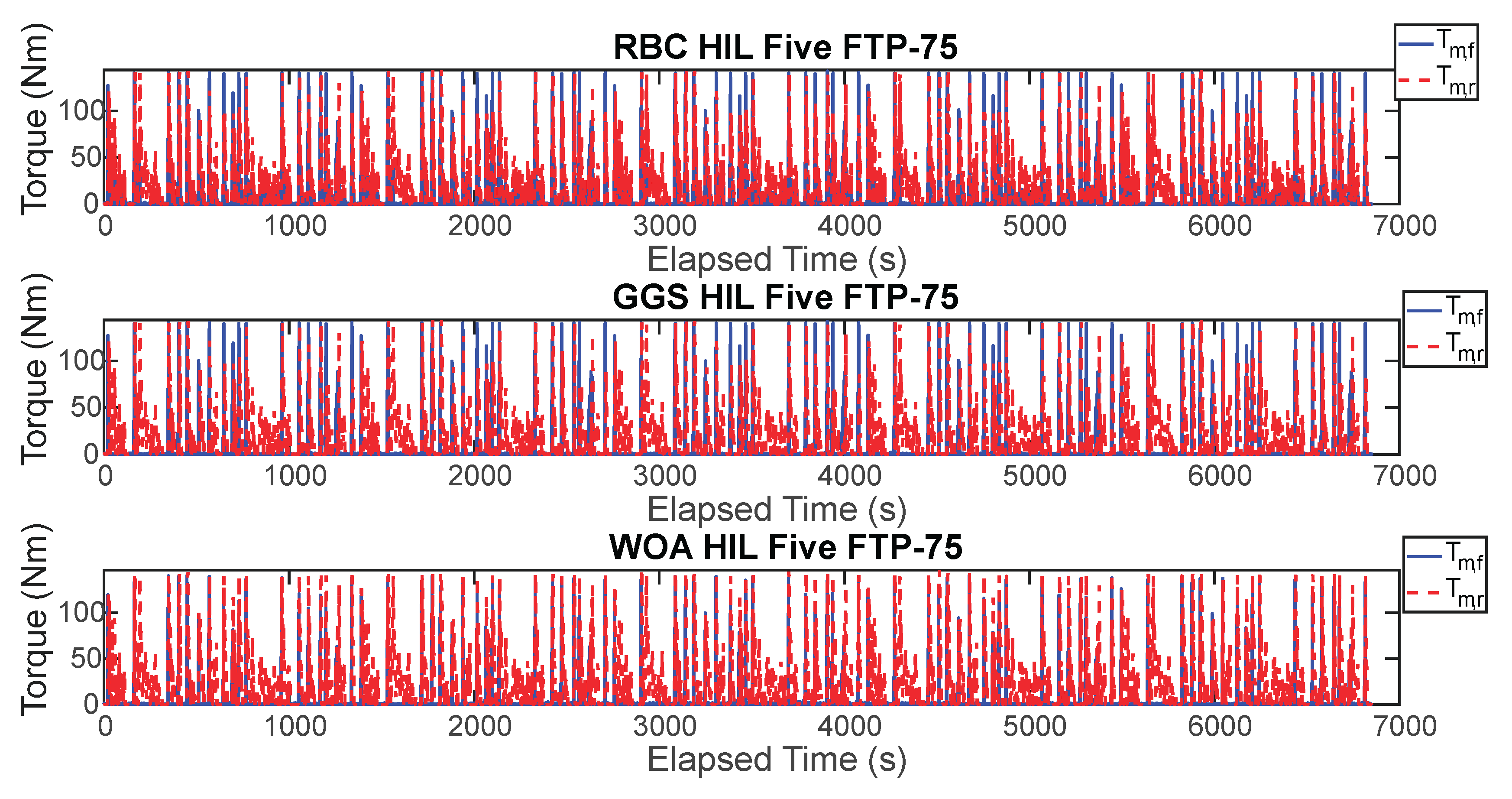

Table 1.
Specification of the electric vehicle.
| Item | Specification | |
|---|---|---|
| Drive Motor | Type | Permanent Magnet Synchronous |
| Maximum Output Power | 250 kW*2 | |
| Maximum Output Torque | 250 Nm@4,750 rpm | |
| Energy Storage Battery | Type | Lithium-ion Battery |
| Rated Voltage | 432 V | |
| Maximum Capacity | 64.58 kWh | |
| Vehicle Parameters | Vehicle Mass | 2373 kg |
| Aerodynamic Drag Coefficient | 0.24 | |
| Frontal Area | 3.5 m2 | |
| Tire Radius | 0.275 m | |
| Rolling Resistance | 0.01 | |
| Final Drive Ratio | 9.78 | |
| Road Friction Coefficient | 0.95 | |
Table 2.
Signal Conversion of the Arduino DUE and Ti C2000 microcontroller.
| Range | Arduino DUE | Conversion | Ti C2000 | ||
|---|---|---|---|---|---|
| -- | Digital | Analog | -- | Digital | Analog |
| Min. | 0 | 0.56 V | DAC | 0 | 0 V |
| Max. | 4095 | 2.76 V | 4095 | 3 V | |
| Min. | 0 | 0 V | ADC | 0 | 0 V |
| Max. | 4095 | 3.3 V | 4095 | 3 V | |
Table 3.
Power distribution mode of the RBC.
| Mode | Condition | Action |
|---|---|---|
| System Ready | Nm | Nm; Nm |
| Low Load | Nm | ; |
| High Load | 50 km/h < | Nm; |
| Safety | = 0 Nm and SOC = 0 | Nm; Nm |
Table 4.
The relevant parameters of the GGS for the front and rear axis motors.
| Parameter | Value |
|---|---|
| 0 : 50 : 250 | |
| 0 : 500 : 13000 | |
| 0 : 0.1 : 1 |
Table 5.
Parameter settings of the WOA.
| Parameter | Value |
|---|---|
| 50 | |
| 340 | |
| [0, 1] Random Value | |
| 1 | |
| [–1, 1] Random Value | |
| )] |
Table 6.
Table 6. Energy Efficiency comparison of grid sizes for GGS.
| Grid Size | Energy Efficiency (km/kWh) |
|---|---|
| 1 | 3.94008 |
| 0.5 | 3.94126 |
| 0.2 | 3.94221 |
| 0.1 | 3.94261 |
| 0.01 | 3.94361 |
| 0.005 | N/A |
| 0.001 | N/A |
Table 7.
Comparison of energy efficiency for different WOA iteration counts and whale population sizes.
Table 7.
Comparison of energy efficiency for different WOA iteration counts and whale population sizes.
| Count | 10 | 100 | 200 | 300 | 400 | |
|---|---|---|---|---|---|---|
| Size | ||||||
| 10 | 3.87261 | 3.87987 | 3.88092 | 3.88101 | N/A | |
| 25 | 3.87666 | 3.88024 | 3.88093 | 3.88101 | N/A | |
| 50 | 3.87822 | 3.88045 | 3.88097 | 3.88102 | N/A | |
| 100 | 3.87824 | 3.88045 | 3.88097 | 3.88102 | N/A | |
| 150 | 3.87824 | 3.88045 | 3.88097 | 3.88102 | N/A | |
Table 8.
Energy efficiency comparison of WOA with 300 and 400 iterations.
| Count | 300 | 320 | 340 | 360 | 380 | |
|---|---|---|---|---|---|---|
| Size | ||||||
| 10 | 3.88102 | 3.88113 | 3.88129 | N/A | N/A | |
Table 9.
Energy efficiency comparison of the pure simulation.
| Strategy | Energy Efficiency (km/kWh) | Improvement Rate (%) |
|---|---|---|
| RBC | 3.5585 | -- |
| GGS | 3.9188 | 9.1 |
| WOA | 3.9063 | 8.9 |
Table 10.
Energy efficiency comparison of the HIL simulation.
| Strategy | Energy Efficiency (km/kWh) | Improvement Rate (%) |
|---|---|---|
| RBC | 3.7510 | -- |
| GGS | 3.9137 | 4.2 |
| WOA | 3.8991 | 3.8 |
Disclaimer/Publisher’s Note: The statements, opinions and data contained in all publications are solely those of the individual author(s) and contributor(s) and not of MDPI and/or the editor(s). MDPI and/or the editor(s) disclaim responsibility for any injury to people or property resulting from any ideas, methods, instructions or products referred to in the content. |
© 2025 by the authors. Licensee MDPI, Basel, Switzerland. This article is an open access article distributed under the terms and conditions of the Creative Commons Attribution (CC BY) license (http://creativecommons.org/licenses/by/4.0/).
Copyright: This open access article is published under a Creative Commons CC BY 4.0 license, which permit the free download, distribution, and reuse, provided that the author and preprint are cited in any reuse.


