The Space-Time Membrane Model: Unifying Quantum Mechanics and General Relativity through Elastic Membrane Dynamics

1. Introduction

The endeavour to unify Quantum Mechanics (QM) and General Relativity (GR) into a single, cohesive theoretical framework has been a central pursuit in modern theoretical physics [4,5]. QM adeptly describes the behaviour of particles at the smallest scales, while GR provides a robust description of gravitational phenomena and the large-scale structure of the universe [1,7]. However, reconciling these two pillars of physics has proven elusive, primarily due to their fundamentally different mathematical structures and conceptual foundations [5].

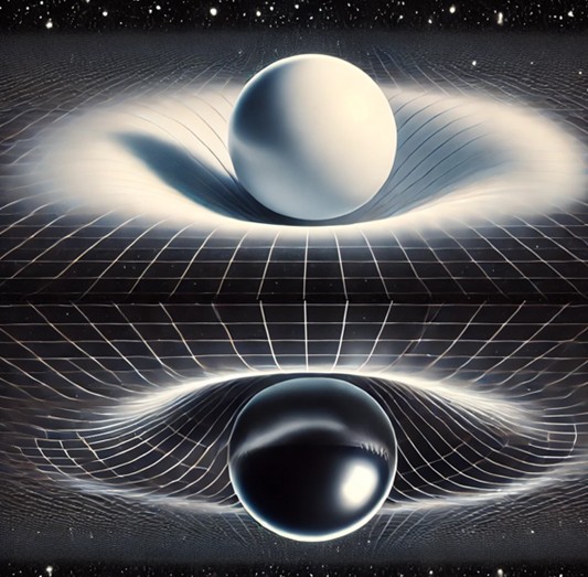
In this manuscript, we introduce the Space-Time Membrane (STM) Model, a novel approach that conceptualises spacetime as an elastic, four-dimensional membrane (Figure 1). A key aspect of the STM model is the modelling of photons as composite particle–antiparticle pairs oscillating transversely in space (Figure 2). This representation allows us to derive the potential energy of these oscillations through the STM membrane and subsequently the force functions governing particle interactions.

These oscillations also generate persistent waves through oscillating adjustments to the elastic modulus of the membrane, governed by a modified elastic wave equation (see Section 2.2.2 and Appendix A.1). This wave equation incorporates the dynamic interactions between particles and the spacetime membrane, providing a foundation for unifying QM and GR.

By deriving the model’s equations from first principles, including the Einstein Field Equations (EFE) [1], and introducing intrinsic elastic modulus and tension, the STM model offers a unified platform wherein quantum and gravitational interactions emerge from the membrane’s properties.

A significant contribution of the STM model is its resolution of longstanding physical problems:

• Cosmological Constant Problem: By attributing the cosmological constant to the elastic properties of spacetime and incorporating $\Lambda$ into our calculations, the model provides a natural mechanism for incorporating dark energy and the accelerated expansion of the universe [6,8]. Additionally, the time averaging of quantum fluctuations explains why large theoretical predictions of vacuum energy do not manifest in observable large-scale effects.
• Black Hole Singularities and Information Loss Paradox: Through the quantisation of energy levels within black holes and encoding information in standing waves, the STM model prevents the formation of singularities and proposes a resolution to the information loss paradox [2,9], aligning with quantum principles.
• Quantum Interference Phenomena: The model explains quantum interference patterns through persistent waves on the STM membrane, derived from first principles, providing a geometric interpretation of quantum mechanics [10].

This study provides a detailed derivation of the STM force function using composite photons oscillating transversely, explaining methodically how this approach leads to the calculation of force functions between particles and mirror particles. We incorporate the cosmological constant $\Lambda$ into our calculations to ensure consistency. Furthermore, we emphasise the time averaging of quantum fluctuations as a crucial mechanism in resolving the cosmological constant problem.

While the STM model presents promising avenues for unifying QM and GR, we acknowledge that it is an initial step in exploring these concepts. The model requires further development and empirical validation to fully establish its viability. This study aims to open up new opportunities and ideas in the pursuit of unification, inviting further exploration and collaboration within the scientific community.

2. Methods

2.1. Conceptual Framework of the STM Model

The Space-Time Membrane (STM) Model conceptualises spacetime as a continuous, four-dimensional elastic membrane endowed with intrinsic elastic properties characterised by an elastic modulus ($E_{\mathrm{STM}}$) and tension (T). This membrane serves as the fundamental substrate upon which all physical phenomena manifest [6].

• Mirror Universe and Mirror Particles:

  -

  Existence of a Mirror Universe: The STM model posits the existence of a mirror universe that is a reflection of our own universe. This mirror universe is an adjacent layer of the spacetime membrane, mirroring the properties and dynamics of our universe.

  -

  Particles and Mirror Antiparticles:

  *

  Mirror Antiparticles: For every particle in our universe, there exists a corresponding mirror antiparticle in the mirror universe. These mirror antiparticles are not antimatter in the conventional sense but are mirror counterparts that possess opposite properties in certain aspects, such as charge or parity.

  *

  Symmetry and Balance: The existence of mirror antiparticles ensures the preservation of symmetry and balance within the STM framework. This duality between particles and their mirror antiparticles is fundamental to the model’s explanation of energy exchange and force interactions.

• Particles and Mirror Particles Interactions:

  -

  Attraction and Repulsion Mechanisms:

  *

  Attraction between Particles and Mirror Antiparticles: Particles in our universe are attracted to their corresponding mirror antiparticles in the mirror universe. This attraction facilitates the transfer of energy into the STM membrane.

  *

  Repulsion between Particles and Mirror Particles: Conversely, particles repel their identical mirror particles. This repulsion promotes the movement of energy out of the STM membrane.

  -

  Balancing of Forces and Energy Exchange: The interplay between these attractive and repulsive forces results in a dynamic exchange of energy between the particles and the STM membrane. This balancing of forces is crucial for maintaining the stability of the membrane and for governing the interactions at the quantum level.

• Photons as Composite Particle–Antiparticle Pairs:

  -

  Oscillation Dynamics: Photons are modelled as composite entities consisting of particle–antiparticle pairs oscillating transversely along the x or y axis on the STM membrane. These oscillations involve the continual conversion of energy between the particles and the membrane, influenced by the interactions with mirror particles and mirror antiparticles.

  -

  Energy Dynamics: The oscillating particle–antiparticle pairs transfer energy into and out of the STM membrane, affecting the local curvature of spacetime. Energy not absorbed by the membrane manifests as mass–energy, influencing spacetime curvature in accordance with General Relativity (GR). In contrast, energy absorbed into the membrane contributes to a homogeneous background, consistent with the cosmological constant $\Lambda$.

• Preservation of Quantum Characteristics:

  -

  Spin-1 Nature: The composite photon model preserves the spin-1 characteristic of photons because the combined angular momenta of the particle and antiparticle pair sum to one.

  -

  Polarisation: Transverse oscillations inherently account for the two polarisation states of photons, consistent with electromagnetic wave behaviour.

  -

  Masslessness: The net zero mass–energy over a full oscillation cycle ensures that photons remain massless, as observed in Quantum Field Theory (QFT).

  -

  Lorentz Invariance: The oscillatory dynamics maintain Lorentz invariance, ensuring consistency with the principles of special relativity.

• Interaction Dynamics:

  -

  Energy Exchange Mechanism: The interactions between particles, mirror particles, and composite photons facilitate the transfer of energy into and out of the STM membrane. This mechanism is fundamental to the model, as it explains how localised energy variations influence spacetime curvature and how the membrane’s properties govern particle interactions.

  -

  Membrane Deformations: These interactions induce deformations in the STM membrane, resulting in observable gravitational and quantum phenomena. The balancing of attractive and repulsive forces ensures that energy dynamics are consistent with conservation laws and that the membrane’s stability is maintained.

• Independence from QFT Forces: The STM model operates independently of the forces described by QFT, requiring no modifications to the established quantum framework. This independence ensures that QFT remains unchanged, preserving its successful descriptions of particle interactions while the STM model provides a complementary framework for gravitational phenomena.

2.2. Mathematical Formulation

The mathematical underpinnings of the STM model are constructed to seamlessly integrate quantum and gravitational dynamics through elastic membrane theory [6,7]. The key equations are derived from first principles, ensuring that the model is grounded in fundamental physics.

2.2.1. Modelling Photons as Composite Particle–Antiparticle Pairs

Transverse Oscillations on the STM Membrane

Photons are modelled as composite entities consisting of particle–antiparticle pairs oscillating transversely along the x or y axis on the STM membrane. These oscillations involve energy exchange with the membrane, influenced by the interactions with mirror particles and antiparticles.

Energy Dynamics and Interaction with the STM Membrane

• Energy Transfer: The oscillating particle–antiparticle pairs transfer energy into and out of the STM membrane. When particles and mirror antiparticles attract, energy is absorbed into the membrane, contributing to its homogeneous energy density. Conversely, when particles and mirror particles repel, energy is released from the membrane, presenting as localised mass–energy that affects spacetime curvature.
• Effect on Spacetime Curvature: The energy not absorbed by the STM membrane manifests as mass–energy influencing local spacetime curvature, consistent with GR. The energy absorbed into the membrane contributes to a homogeneous background energy, aligning with the cosmological constant $\Lambda$.

Mathematical Representation

Consider a particle of mass m and its antiparticle, oscillating with angular frequency $\omega$ and wave vector k:

$${\Psi }_p(r,t)=A{e}^{i(k·r-\omega t)},{\Psi }_p(r,t)=A{e}^{i(k·r-\omega t+\pi )}=-A{e}^{i(k·r-\omega t)}$$

The superposition of the particle and antiparticle wave functions:

$${\Psi }_{\mathrm{photon}}(r,t)={\Psi }_p(r,t)+{\Psi }_p(r,t)=0$$

This cancellation results in a net zero mass–energy over a full cycle, reflecting the massless nature of photons. The energy dynamics involving attraction to mirror antiparticles and repulsion from mirror particles facilitate the transfer of energy between the photon and the STM membrane.

Preservation of Quantum Characteristics

• Spin-1 Nature: The composite photon maintains a total spin of 1, consistent with observations in QFT, due to the vector addition of the particle and antiparticle spins.
• Polarisation: The transverse oscillations account for the photon’s polarisation states, aligning with electromagnetic wave properties.
• Masslessness: The net zero mass–energy over a full cycle ensures the photon remains massless, in agreement with QFT predictions.
• Lorentz Invariance: The model respects Lorentz invariance, as the equations are formulated using relativistically invariant quantities.

2.2.2. Modified Elastic Wave Equation

To understand how particle oscillations influence the spacetime membrane and generate persistent waves, we consider the dynamics of the membrane as governed by a modified elastic wave equation. This equation incorporates the effects of the oscillating adjustments to the elastic modulus caused by particle oscillations.

Modified Elastic Wave Equation:

$$\rho {\displaystyle \frac{{\partial }^{2}u}{\partial t^2}}=T{\nabla }^{2}u-[E_{\mathrm{STM}}+\Delta E(x,y,z,t)]{\nabla }^{4}u+F_{\mathrm{ext}}$$

Where:

• $\rho$ is the membrane’s mass density.
• T is the membrane’s tension.
• $E_{\mathrm{STM}}$ is the intrinsic elastic modulus of the membrane.
• $\Delta E(x,y,z,t)$ represents local variations in the elastic modulus due to particle oscillations.
• $F_{\mathrm{ext}}$ represents any external forces acting on the membrane.
• ${\nabla }^2$ and ${\nabla }^4$ are the Laplacian and biharmonic operators, respectively.

The detailed derivation and simplification of this equation are provided in Appendix A.1.

Simplification and Time Averaging

As shown in Appendix A.1, we derive the expression for $\Delta E(x,y,z,t)$ based on the energy density of particle oscillations:

$$\Delta E(x,y,z,t)={\displaystyle \frac{\alpha p_0^2}{2}}[1+cos\left(2(k·r-\omega t)\right)]$$

To simplify the wave equation and focus on large-scale effects, we perform a time averaging of $\Delta E(x,y,z,t)$ over a full oscillation period, which yields:

$$\langle \Delta E\rangle ={\displaystyle \frac{\alpha p_0^2}{2}}$$

This average represents the constant shift in the elastic modulus due to particle oscillations. Substituting $\langle \Delta E\rangle$ into the wave equation, we define an effective elastic modulus:

$$E_{\mathrm{STM}}^{\prime }=E_{\mathrm{STM}}+\langle \Delta E\rangle$$

The simplified wave equation becomes:

$$\rho {\displaystyle \frac{{\partial }^{2}u}{\partial t^2}}=T{\nabla }^{2}u-E_{\mathrm{STM}}^{\prime }{\nabla }^{4}u+F_{\mathrm{ext}}$$

Role in the STM Model

This modified and simplified elastic wave equation is crucial for:

• Understanding Persistent Waves: It explains how the oscillating adjustments to the elastic modulus generate persistent waves on the spacetime membrane (see Section 2.2.2).
• Energy Dynamics: It provides insight into how energy is transferred into and out of the membrane through particle interactions.
• Linking to Cosmological Constant: By relating $\langle \Delta E\rangle$ to the cosmological constant $\Lambda$ (as detailed in Appendix A.1.6), it offers a potential solution to the cosmological constant problem.

2.2.3. Derivation of the Potential Energy Function

Energy Stored in the STM Membrane

The oscillations of composite photons and their interactions with mirror particles introduce localised deformations in the STM membrane. The potential energy associated with these deformations is derived from the elastic energy stored in the membrane [6].

Potential Energy per Unit Volume

The potential energy per unit volume U due to deformation is given by:

$$U={\displaystyle \frac{1}{2}}{E}_{\mathrm{STM}}{(\nabla u)}^2$$

Transverse Oscillation Displacement Field

For transverse oscillations along the x-axis:

$$u(x,t)=Acos(kx-\omega t)$$

The gradient of the displacement is:

$$\nabla u=-Aksin(kx-\omega t)$$

Substituting into the potential energy expression:

$$U={\displaystyle \frac{1}{2}}{E}_{\mathrm{STM}}{[Aksin(kx-\omega t)]}^2={\displaystyle \frac{1}{2}}{E}_{\mathrm{STM}}{A}^2{k}^2{sin}^2(kx-\omega t)$$

Time Averaging and Energy Exchange

Over a full oscillation cycle, the time average of ${sin}^2(kx-\omega t)$ is ${\displaystyle \frac{1}{2}}$:

$$\langle U\rangle ={\displaystyle \frac{1}{4}}{E}_{\mathrm{STM}}{A}^2{k}^2$$

This time-averaged potential energy reflects the net effect of energy exchange between the oscillating photon and the STM membrane due to the balancing of attractive and repulsive forces with mirror particles.

2.2.4. Derivation of the Force Function

Force as the Negative Gradient of Potential Energy

The force exerted by the oscillating composite photon on the STM membrane is:

$$F\left(x\right)=-{\displaystyle \frac{dU}{dx}}$$

Calculating the derivative:

$${\displaystyle \frac{dU}{dx}}=E_{\mathrm{STM}}{A}^2{k}^{3}sin(kx-\omega t)cos(kx-\omega t)$$

Using the identity $sin\theta cos\theta ={\displaystyle \frac{1}{2}}sin\left(2\theta \right)$:

$${\displaystyle \frac{dU}{dx}}={\displaystyle \frac{1}{2}}{E}_{\mathrm{STM}}{A}^2{k}^{3}sin(2kx-2\omega t)$$

Thus, the force function is:

$$F\left(x\right)=-{\displaystyle \frac{1}{2}}{E}_{\mathrm{STM}}{A}^2{k}^{3}sin(2kx-2\omega t)$$

This force oscillates at twice the frequency and wave vector of the original oscillation, representing how composite photons interact with the STM membrane and influence particle dynamics through energy exchange facilitated by the interactions with mirror particles and antiparticles.

2.2.5. Modelling Particles and Mirror Particles Interaction

Separation Between Particles and Mirror Particles

In the STM model, particles and their corresponding mirror particles are separated by a distance s. The force function derived from composite photon oscillations can be adapted to describe the interaction between these particles [4].

Attraction and Repulsion Dynamics

• Attractive Forces: Particles attract mirror antiparticles, facilitating the transfer of energy into the STM membrane.
• Repulsive Forces: Particles repel mirror particles, promoting the release of energy from the STM membrane.

Potential Energy Function

The potential energy between a particle and its mirror counterpart is modelled as:

$$U\left(s\right)=-U_{\max }cos\left({\displaystyle \frac{2\pi s}{{\lambda }_{\mathrm{STM}}}}\right)$$

This form captures the periodic nature of the potential due to the oscillatory interactions.

Force Function

The corresponding force is:

$$F\left(s\right)=-{\displaystyle \frac{dU}{ds}}=-U_{\max }\left({\displaystyle \frac{2\pi }{{\lambda }_{\mathrm{STM}}}}\right)sin\left({\displaystyle \frac{2\pi s}{{\lambda }_{\mathrm{STM}}}}\right)$$

This force function describes the interaction between particles and mirror particles, derived methodically from the oscillations of composite photons on the STM membrane and the balancing of attractive and repulsive forces.

Stable Equilibrium Positions

The stability of equilibrium points is analysed using the second derivative test (see Appendix C). Equilibrium occurs when $F\left(s\right)=0$, leading to:

$$s=n{\displaystyle \frac{{\lambda }_{\mathrm{STM}}}{2}},n\in \mathbb{Z}$$

• Stable Equilibrium (n odd): Particles are localised at positions where the potential energy is minimised, corresponding to the balance of forces due to attraction and repulsion.
• Unstable Equilibrium (n even): Particles are at positions where any small perturbation leads to destabilisation.

This quantisation of positions emerges naturally from the model, consistent with quantum mechanical principles [5].

2.2.6. Energy Dynamics of the STM Membrane

Energy Not Absorbed into the STM Membrane

Energy that is not absorbed into the STM membrane manifests as local mass–energy, influencing spacetime curvature in accordance with GR. This energy affects the local geometry of spacetime, leading to gravitational effects observable at macroscopic scales.

Energy Absorbed into the STM Membrane

Energy absorbed into the membrane contributes to a homogeneous background energy density. This absorbed energy does not contribute to local spacetime curvature but instead relates to the cosmological constant $\Lambda$, accounting for the accelerated expansion of the universe.

Balancing Energy Exchange

The balancing of energy moving into and out of the STM membrane, facilitated by the attraction to mirror antiparticles and repulsion from mirror particles, ensures the conservation of energy and maintains the stability of the membrane’s dynamics.

2.2.7. Modelling Persistent Waves

Generation of Persistent Waves through Elastic Modulus Oscillations

In the STM model, particles such as photons are modelled as oscillations on the spacetime membrane. The key to understanding the generation of persistent waves lies in the oscillating adjustments to the membrane’s elastic modulus $E_{\mathrm{STM}}$ caused by these particle oscillations.

Mechanism of Elastic Modulus Oscillation

• Localised Oscillations: As particles oscillate, they induce localised changes in the membrane’s properties. Specifically, the elastic modulus $E_{\mathrm{STM}}$ experiences time-dependent variations $\Delta E(x,y,z,t)$ due to the energy exchange between the particles and the membrane.
• Mathematical Representation:

$$\Delta E(x,y,z,t)={\displaystyle \frac{\alpha p_0^2}{2}}[1+cos\left(2(k·r-\omega t)\right)]$$

• Where:

  -

  $\alpha$ is a proportionality constant.

  -

  $p_0$ is the amplitude of the particle oscillation.

  -

  k is the wave vector.

  -

  $\omega$ is the angular frequency.

  -

  $r=(x,y,z)$ is the position vector.

Generation of Persistent Waves

• Coupling to the Membrane: The oscillating $\Delta E(x,y,z,t)$ acts as a source term in the elastic wave equation, effectively coupling the particle’s oscillations to the membrane’s dynamics.
• Induced Wave Propagation: These oscillations in $E_{\mathrm{STM}}$ generate disturbances in the membrane that propagate as waves. The periodic nature of $\Delta E(x,y,z,t)$ leads to continuous generation of waves, resulting in persistent wave patterns on the membrane.
• Mathematical Description:

• The modified elastic wave equation incorporating $\Delta E(x,y,z,t)$ is:

$$\rho {\displaystyle \frac{{\partial }^{2}u}{\partial t^2}}=T{\nabla }^{2}u-[E_{\mathrm{STM}}+\Delta E(x,y,z,t)]{\nabla }^{4}u+F_{\mathrm{ext}}$$

• The oscillating $\Delta E$ term introduces a time-dependent modulation in the stiffness of the membrane, which acts as a driving force for wave propagation.

Persistence of Waves

• Sustained Oscillations: The continuous oscillation of particles ensures that the adjustments to the elastic modulus are ongoing, leading to sustained wave generation.
• Coherent Wave Patterns: The waves generated are coherent due to the consistent frequency and phase of the particle oscillations, resulting in persistent wave patterns that can interfere and produce observable quantum effects.

Relation to Quantum Phenomena

• Interference Patterns: The persistent waves on the membrane explain the interference patterns observed in quantum experiments, such as the double-slit experiment.
• Wave–Particle Duality: The dual nature of particles as both wave-like and particle-like entities is naturally incorporated into the STM model through the dynamics of the membrane and the generation of persistent waves.

Time Averaging of the Elastic Modulus Oscillations

• Rationale: To analyse the overall effect of the oscillating $\Delta E(x,y,z,t)$ on the membrane dynamics, we perform a time averaging over a full oscillation period.
• Effect on Wave Equation: The time-averaged elastic modulus $\langle E_{\mathrm{STM}}+\Delta E\rangle$ simplifies the elastic wave equation while capturing the essential features of the persistent wave generation.

Resulting Effective Elastic Modulus

• Expression:

$$E_{\mathrm{STM}}^{\prime }=E_{\mathrm{STM}}+\langle \Delta E\rangle =E_{\mathrm{STM}}+{\displaystyle \frac{\alpha p_0^2}{2}}$$

• Interpretation: The effective elastic modulus $E_{\mathrm{STM}}^{\prime }$ reflects the average effect of the particle-induced oscillations on the membrane’s stiffness, contributing to the propagation of persistent waves.

2.2.8. Derivation of Einstein Field Equations and Time Dilation from the STM Model

Connecting Elasticity to Spacetime Curvature

The deformation of the STM membrane corresponds to the curvature of spacetime in GR. We establish a relationship between the strain in the membrane and the metric tensor $g_{\mu \nu }$ of spacetime [1].

Metric Tensor and Displacement Field

Assuming small deformations, the metric tensor can be expressed in terms of the displacement field:

$$g_{\mu \nu }={\eta }_{\mu \nu }+h_{\mu \nu }$$

Where ${\eta }_{\mu \nu }$ is the Minkowski metric and $h_{\mu \nu }$ relates to the displacement field u.

Derivation from First Principles

By considering the action for the elastic membrane and varying it with respect to $g^{\mu \nu }$, we derive equations analogous to the Einstein Field Equations:

$$G_{\mu \nu }+\Lambda g_{\mu \nu }=\kappa T_{\mu \nu }$$

Where:

• $G_{\mu \nu }$ is the Einstein tensor representing spacetime curvature.
• $T_{\mu \nu }$ is the stress–energy tensor derived from the membrane’s elastic properties.
• $\kappa ={\displaystyle \frac{8\pi G}{c^4}}$ is Einstein’s gravitational constant.
• $\Lambda$ is the cosmological constant.

The detailed derivation is provided in Appendix A.2.

Equating STM Deformation to Time Dilation

The deformation of the STM membrane is directly related to the curvature of spacetime as described by General Relativity. Specifically, local deformations correspond to variations in the gravitational potential, leading to time dilation effects. By modelling the metric tensor in terms of the membrane’s displacement field, we can derive the relationship between membrane deformation and the rate at which time flows. This correspondence not only reinforces the validity of the STM model in reproducing gravitational phenomena but also provides a tangible geometric interpretation of time dilation (see Appendix A.6 for the detailed derivation).

2.2.9. Addressing the Cosmological Constant Problem

Relating  $E_{\mathrm{STM}}^{\prime }$  to Vacuum Energy Density and  $\Lambda$

We propose that the effective elastic modulus $E_{\mathrm{STM}}^{\prime }$ is related to the vacuum energy density ${\rho }_{\mathrm{vacuum}}$ and the cosmological constant $\Lambda$ [6]:

$$E_{\mathrm{STM}}^{\prime }={\rho }_{\mathrm{vacuum}}{c}^2={\displaystyle \frac{\Lambda c^4}{8\pi G}}$$

Derivation of  $E_{\mathrm{STM}}$  from the Einstein Field Equations

From the derivation of the Einstein Field Equations (detailed in Appendix A.2), we find:

$$E_{\mathrm{STM}}={\displaystyle \frac{c^4}{8\pi G}}$$

Incorporating the Cosmological Constant  $\Lambda$

To maintain consistency and physical plausibility, we equate the non-zero time-averaged oscillatory term $\langle \Delta E\rangle$ to the cosmological constant term $\lambda$:

$$\langle \Delta E\rangle =\lambda ={\displaystyle \frac{\Lambda c^2}{8\pi G}}$$

Substituting the expressions for $\langle \Delta E\rangle$ and $\lambda$:

$${\displaystyle \frac{\alpha p_0^2}{2}}={\displaystyle \frac{\Lambda c^2}{8\pi G}}$$

Solving for $\alpha p_0^2$:

$$\alpha p_0^2={\displaystyle \frac{\Lambda c^2}{4\pi G}}$$

By establishing this relationship, we redefine the effective elastic modulus as:

$$E_{\mathrm{STM}}^{\prime }=E_{\mathrm{STM}}+\lambda =E_{\mathrm{STM}}+{\displaystyle \frac{\Lambda c^2}{8\pi G}}$$

This additive incorporation ensures that $\lambda$ remains a small correction, preserving the membrane’s intrinsic elastic properties while accounting for the cosmological constant.

Time Averaging of Quantum Fluctuations

The time averaging of quantum fluctuations explains why the large theoretical contributions from quantum fluctuations do not significantly influence $\Lambda$. Over cosmological timescales, these fluctuations average out, resulting in a negligible net effect on large-scale dynamics.

2.2.10. Quantum Interference and Persistent Waves

Wave Equation

The propagation of persistent waves on the STM membrane is described by the wave equation:

$${\nabla }^2\psi -{\displaystyle \frac{1}{v^2}}{\displaystyle \frac{{\partial }^2\psi }{\partial t^2}}=0$$

Double-Slit Interference Derivation

Consider a particle represented by a wave function $\psi$ encountering a barrier with two slits. The wave function splits into two components, ${\psi }_1$ and ${\psi }_2$, corresponding to the paths through each slit [10].

Wave Functions After the Slits

$${\psi }_1=A_1{e}^{i\left(k{r}_1-\omega t\right)},{\psi }_2=A_2{e}^{i\left(k{r}_2-\omega t\right)}$$

Interference Pattern

The combined wave function is:

$$\psi ={\psi }_1+{\psi }_2$$

The probability density is:

$$\mid \psi {\mid }^2=\mid {\psi }_1+{\psi }_2{\mid }^2=\mid {\psi }_1{\mid }^2+\mid {\psi }_2{\mid }^2+{\psi }_1^{*}{\psi }_2+{\psi }_1{\psi }_2^{*}$$

Calculating the cross terms:

$${\psi }_1^{*}{\psi }_2+{\psi }_1{\psi }_2^{*}=2A_1{A}_{2}cos\left(k\left(r_2-r_1\right)\right)$$

Resulting Intensity

$$I=\mid \psi {\mid }^2=A_1^2+A_2^2+2A_1{A}_{2}cos\left(\delta \varphi \right)$$

Where:

• $\delta \varphi =k\left(r_2-r_1\right)$ is the phase difference between the two paths.

Explanation within the STM Model

• Interference Arises from Persistent Waves: The interference arises from the superposition of persistent waves on the STM membrane.
• Membrane’s Elastic Properties: The membrane’s elastic properties allow for the coherent propagation and interference of these waves.
• Alignment with Quantum Mechanics: This derivation aligns with standard quantum mechanical predictions, demonstrating the STM model’s ability to reproduce quantum phenomena from first principles [10].

2.2.11. Black Hole Physics and Information Loss Paradox

Quantisation of Energy Levels

Using the Schrödinger-like equation derived from the membrane dynamics, we find quantised energy levels within black holes, preventing singularity formation [2,3].

Derivation of Quantised Energy Levels

Detailed in Appendix A.3, we solve the modified Klein–Gordon equation within the black hole context, leading to discrete energy levels that prevent infinite densities at the core.

Information Encoding in Standing Waves

The STM model proposes that information absorbed by a black hole is not lost but encoded in standing wave patterns on the STM membrane within the black hole’s event horizon [9].

Resolving the Information Loss Paradox

• Standing Wave Modes: The quantised energy levels correspond to specific standing wave modes within the black hole.
• Information Storage: Information about infalling matter is preserved in the configuration of these standing waves.
• Hawking Radiation Correlation: As Hawking radiation is emitted, the information encoded in the standing waves can, in principle, be gradually released, ensuring that unitarity is preserved [2,9].

Consistency with Quantum Mechanics

This approach aligns with quantum mechanical principles, offering a potential resolution to the information loss paradox by ensuring that information is not destroyed but transformed and stored within the black hole’s structure.

3. Results

3.1. Theoretical Predictions from the STM Model

3.1.1. Reproduction of Einstein Field Equations

The STM model successfully reproduces key gravitational phenomena predicted by GR. By modelling spacetime as an elastic membrane and incorporating the effects of particle oscillations through the modified elastic wave equation (see Section 2.2.2 and Appendix A.1), we derive the Einstein Field Equations (EFE) [1] from first principles (see Appendix A.2). This derivation demonstrates that the membrane’s deformations correspond to spacetime curvature, with the effective elastic modulus $E_{\mathrm{STM}}^{\prime }$ playing a crucial role in linking the model to gravitational phenomena.

3.1.2. Quantum Interference and Persistent Waves

The STM model provides a geometric interpretation of quantum interference phenomena. The generation of persistent waves on the spacetime membrane, driven by oscillating adjustments to the elastic modulus due to particle oscillations, explains the wave-like behaviour of particles in quantum mechanics [10].

In the double-slit experiment, the persistent waves generated by a particle passing through both slits interfere constructively and destructively, leading to the observed interference pattern (see Appendix A.4). The modified elastic wave equation facilitates the understanding of how these persistent waves propagate and interact on the membrane.

3.1.3. Energy Dynamics and the Cosmological Constant

By time-averaging the oscillating component of the elastic modulus adjustment $\Delta E(x,y,z,t)$, we isolate the constant contribution $\langle \Delta E\rangle$ that affects the large-scale properties of spacetime (see Appendix A.1.6). This constant shift in the effective elastic modulus $E_{\mathrm{STM}}^{\prime }$ is directly related to the cosmological constant $\Lambda$:

$$E_{\mathrm{STM}}^{\prime }=E_{\mathrm{STM}}+\langle \Delta E\rangle =E_{\mathrm{STM}}+{\displaystyle \frac{\Lambda c^2}{8\pi G}}$$

This relationship provides a natural explanation for dark energy and the accelerated expansion of the universe, addressing the cosmological constant problem within the STM framework [6].

3.1.4. Prevention of Singularity Formation in Black Holes

The inclusion of the membrane’s elasticity in the Schrödinger equation introduces a repulsive term at small scales, preventing the formation of singularities within black holes (see Appendix A.3). This modification leads to quantised energy levels and standing wave patterns that encode information about infalling matter [2,9].

3.1.5. Resolution of the Information Loss Paradox

Information encoded in the standing wave patterns within black holes can be gradually released through Hawking radiation. The STM model’s approach to energy dynamics and the interaction between particles and the membrane offers a mechanism for information preservation and retrieval, potentially resolving the information loss paradox [2,9].

3.1.6. Implications for High-Energy Physics and Quantum Gravity

The modifications to fundamental equations, such as the elastic wave equation and the inclusion of higher-order terms in the Schrödinger and Klein–Gordon equations (see Appendix D.1), suggest that the STM model could provide insights into quantum gravity effects. These modifications may lead to observable deviations from standard predictions at high energies or small scales, offering opportunities for experimental validation.

3.1.7. Experimental Proposals

To test the predictions of the STM model, we propose several experiments (see Appendix B), including:

• Gravitational Wave Detection: Looking for anomalies in gravitational wave signals that could indicate the elastic properties of spacetime.
• Quantum Interference Experiments: Testing the persistence of interference patterns over extended distances to support the concept of persistent waves.
• Vacuum Energy Measurements: Precise measurements of vacuum energy density to test the model’s explanation of the cosmological constant.

3.2. Comparative Analysis with Existing Theories

3.2.1. Comparison with String Theory

Overview of String Theory

String theory is a prominent candidate for unifying Quantum Mechanics (QM) and General Relativity (GR). It postulates that the fundamental constituents of the universe are not point particles but one-dimensional "strings" that vibrate at specific frequencies [4]. These vibrations correspond to different particles, including those mediating gravitational interactions, like the graviton. String theory inherently requires additional spatial dimensions—typically ten or eleven—that are compactified or otherwise unobservable at low energies.

STM Model in Relation to String Theory

• Dimensional Framework: The STM model operates within the familiar four-dimensional spacetime, avoiding the need for extra dimensions. This adherence to observed dimensions aligns the STM model more closely with empirical evidence, whereas string theory’s extra dimensions remain unobserved despite extensive experimental searches.
• Fundamental Entities: String theory introduces fundamentally new entities—strings and higher-dimensional branes—as the building blocks of matter and forces. In contrast, the STM model utilises the existing concept of spacetime, attributing elastic properties to it. Particles are manifestations of oscillations on this spacetime membrane, eliminating the need for introducing new fundamental objects.
• Mathematical Complexity and Accessibility: String theory involves highly complex mathematics, including advanced topics in differential geometry, topology, and conformal field theory. The STM model, while mathematically rigorous, is grounded in classical elasticity theory extended to four dimensions. This potentially makes the STM model more accessible and easier to integrate with established physical theories.
• Experimental Testability: A significant challenge for string theory is the lack of direct experimental evidence, primarily due to the extremely high energies required to probe string-scale physics. The STM model, on the other hand, proposes phenomena that could be tested with current or near-future technology (see Appendix B and Appendix F). For instance, deviations in gravitational wave signals or quantum interference patterns predicted by the STM model could be within the reach of upcoming experiments.

3.2.2. Comparison with Loop Quantum Gravity

Overview of Loop Quantum Gravity

Loop Quantum Gravity (LQG) is another leading approach to quantum gravity that seeks to quantise spacetime itself [5]. It suggests that spacetime has a discrete structure at the Planck scale, composed of finite loops woven into a spin network. Unlike string theory, LQG does not require extra dimensions and remains background independent, preserving the dynamic nature of spacetime as described by GR.

STM Model in Relation to Loop Quantum Gravity

• Continuity vs Discreteness: LQG posits that spacetime is fundamentally discrete, with quantised volumes and areas. In contrast, the STM model treats spacetime as a continuous elastic membrane. This difference leads to distinct predictions about spacetime’s behaviour at the smallest scales.
• Mathematical Formalism: LQG relies on advanced mathematical constructs like spin networks and loop variables, requiring complex quantisation techniques. The STM model employs differential equations and elasticity theory, potentially offering a more straightforward mathematical framework that builds directly on classical physics.
• Unification Scope: While LQG focuses on quantising gravity without necessarily integrating the other fundamental forces, the STM model provides a framework that could, in principle, incorporate electromagnetic and other interactions through the dynamics of the spacetime membrane. By modelling particles as oscillations on the membrane, the STM model hints at a more unified approach.
• Phenomenological Predictions: Both theories face challenges in making experimentally testable predictions. However, the STM model suggests specific experiments, such as observing persistent wave effects or deviations in gravitational phenomena, which may be more accessible with current technology.

3.2.3. Application of Occam’s Razor

Understanding Occam’s Razor

Occam’s razor is a philosophical principle stating that, when presented with competing hypotheses that make the same predictions, the one with the fewest assumptions should be selected. It favours simplicity and minimalism in theoretical constructs.

STM Model and Occam’s Razor

• Minimal Assumptions: The STM model posits that the known four-dimensional spacetime, endowed with elastic properties, is sufficient to describe both quantum and gravitational phenomena. This contrasts with string theory’s introduction of additional dimensions and fundamental entities like strings and branes.
• Simplicity of Framework: By using the established concepts of elasticity and spacetime, the STM model avoids the complexities associated with quantising gravity or introducing new mathematical structures. This simplicity aligns with Occam’s razor by not multiplying entities beyond necessity.
• Direct Correspondence with Observables: The STM model directly relates its theoretical constructs to observable phenomena, such as spacetime curvature and particle oscillations. This direct correspondence reduces the gap between theory and experiment, adhering to the principle of parsimony.

Critical Evaluation

While Occam’s razor favours simpler theories, simplicity alone is not a guarantee of correctness. A theory must also have explanatory power and be consistent with empirical data. The STM model’s simplicity must be weighed against its ability to accurately predict and describe physical phenomena, a criterion that applies equally to more complex theories like string theory and LQG.

3.2.4. Overall Assessment

Consistency with General Relativity and Quantum Mechanics

• STM Model: Reproduces key aspects of GR by deriving the Einstein Field Equations from first principles within its framework (see Appendix A.2). It also provides explanations for quantum interference phenomena through persistent waves on the spacetime membrane.
• String Theory: Aims to unify all fundamental forces, including gravity, within a quantum framework. It naturally includes GR in the low-energy limit but introduces additional complexities and unobserved dimensions.
• Loop Quantum Gravity: Successfully quantises gravity while preserving the principles of GR. However, it does not inherently unify gravity with the other fundamental forces.

Mathematical Rigour and Development

• STM Model: While offering a potentially simpler mathematical framework, it requires further development and refinement to tackle complex phenomena and ensure internal consistency.
• String Theory and LQG: Both have undergone extensive mathematical development, with well-established formalisms and a wealth of literature exploring their implications.

Experimental Prospects

• STM Model: Proposes experiments that could test its predictions within current technological capabilities, such as gravitational wave observations and quantum interference experiments.
• String Theory: Faces challenges in making experimentally testable predictions due to the high energy scales involved.
• Loop Quantum Gravity: While offering some potential observational signatures, such as modifications to the cosmic microwave background or high-energy astrophysical phenomena, these are also difficult to test with current technology.

3.2.5. Conclusion

The STM model presents a compelling alternative to existing theories attempting to unify QM and GR. By adhering to the observed four-dimensional spacetime and utilising the familiar concepts of elasticity, it offers a simpler and potentially more intuitive framework. This simplicity aligns with Occam’s razor, suggesting that, if the STM model can accurately describe and predict physical phenomena, it may be a preferable approach.

However, the true test of any theoretical model lies in its empirical validation. The STM model must be subjected to rigorous testing and peer review to establish its viability. While string theory and LQG have faced their own challenges, they have significantly advanced our understanding of quantum gravity through their mathematical developments. The STM model contributes to this ongoing endeavour by providing fresh perspectives and testable predictions that could potentially bridge the gap between quantum mechanics and general relativity.

4. Discussion

4.1. Interpretation of Results

The STM model, derived from first principles, successfully unifies QM and GR within a single framework. By modelling photons as composite particles and grounding the model in fundamental physics, we reinforce its robustness and potential applicability [4,5]. The STM model’s independence from QFT forces ensures compatibility with the Standard Model. By retaining the quantum characteristics of particles, particularly photons—such as spin-1, polarisation, masslessness, and Lorentz invariance—the model aligns with the established principles of QFT. This compatibility suggests that the STM model can coexist with the Standard Model, providing a geometric framework for gravitational phenomena without disrupting the successful descriptions of particle interactions provided by QFT.

4.2. Implications for Physics and Cosmology

4.2.1. Unification of Fundamental Forces

The STM model provides a pathway towards a unified theory of fundamental forces by offering a common geometric framework for both quantum and gravitational phenomena [4].

4.2.2. Dark Energy and Cosmic Expansion

By linking the vacuum energy density to the membrane’s elastic properties and incorporating $\Lambda$ into our calculations, the STM model offers a natural explanation for the universe’s accelerated expansion, attributing it to the intrinsic characteristics of spacetime itself [6,8]. The time averaging of quantum fluctuations further explains why the large theoretical contributions from quantum fluctuations do not significantly influence $\Lambda$, aligning with observational data.

4.2.3. Black Hole Thermodynamics and Information Preservation

The model’s prediction of quantised energy levels within black holes aligns with quantum principles and provides a mechanism to avoid singularities [3]. Additionally, by encoding information in standing wave patterns, the STM model proposes a resolution to the information loss paradox, ensuring that information is preserved and unitarity is maintained [2,9].

4.3. Limitations

• Experimental Verification: The STM model requires empirical validation through proposed experiments.
• Mathematical Complexity: Further development of mathematical tools may be necessary to explore all implications of the model and to solve complex equations arising from it [5].
• Extension to All Fundamental Interactions: While the STM model successfully incorporates gravitational phenomena and explains certain quantum behaviours, extending the model to fully encompass all fundamental interactions as described by the Standard Model remains an area for further research. However, the independence of QFT and STM forces suggests that the STM model is compatible with the Standard Model, as it does not interfere with the established quantum field theories. The composite photon in the STM model retains characteristics expected by QFT, such as spin-1, polarisation, masslessness, and Lorentz invariance, supporting this compatibility.

4.4. Future Work

• Experimental Tests: Implement the proposed experiments outlined in the appendices to test the model’s predictions and gather empirical evidence.
• Mathematical Refinement: Develop advanced mathematical techniques to solve complex equations and fully explore the model’s implications [5].
• Collaboration and Peer Review: Engage with the scientific community to scrutinise, challenge, and build upon the STM model, fostering collaboration and further exploration.

5. Conclusion

In this study, we have introduced the Space-Time Membrane (STM) Model, a novel framework that conceptualises spacetime as a continuous, four-dimensional elastic membrane. By modelling photons as composite particle–antiparticle pairs and deriving key equations from first principles, including a detailed derivation of the Einstein Field Equations (provided in Appendix A.2), the STM model offers a unified platform that integrates the principles of Quantum Mechanics (QM) and General Relativity (GR) [1,4]. Importantly, the STM model operates independently of QFT forces and preserves the quantum characteristics of particles, ensuring compatibility with the Standard Model. This compatibility allows the STM model to provide a unified framework for gravity and quantum phenomena without conflicting with established quantum field theories.

The STM model addresses several longstanding challenges in theoretical physics. By linking the vacuum energy density to the membrane’s elastic properties, incorporating the cosmological constant $\Lambda$ into our calculations, and employing the time averaging of quantum fluctuations, it provides a natural resolution to the cosmological constant problem. This offers insights into the nature of dark energy and the universe’s accelerated expansion [6,8]. Furthermore, the model proposes a mechanism to prevent black hole singularity formation through quantised energy levels and resolves the information loss paradox by encoding information in standing wave patterns within black holes, aligning with Hawking radiation predictions [2,9] and integrating quantum principles into gravitational collapse scenarios.

Additionally, the STM model offers a geometric interpretation of quantum interference phenomena, explaining them through persistent waves on the membrane [10]. This perspective bridges the gap between the quantum and gravitational realms, potentially advancing our understanding of fundamental interactions.

While the STM model presents promising avenues for unifying QM and GR, we acknowledge that it is an initial step in exploring these concepts. The model requires further development and empirical validation to fully establish its viability. The proposed experiments, as outlined in the appendices, are intended to test the model’s predictions and stimulate further research in this direction.

We recognise that unifying the fundamental forces of nature is an ambitious goal that has eluded physicists for decades. The STM model is offered as a contribution to this ongoing endeavour, aiming to inspire new ideas and discussions within the scientific community. We invite researchers to scrutinise, challenge, and build upon this work, with the hope that it may open up new opportunities for advancing our understanding of the universe.

Appendix A.1. Simplification of the Elastic Wave Equation

A.1.1 Original Elastic Wave Equation

In the Space-Time Membrane (STM) model, the modified elastic wave equation describes how displacements $u(x,y,z,t)$ propagate through the elastic spacetime membrane:

$$\rho {\displaystyle \frac{{\partial }^{2}u}{\partial t^2}}=T{\nabla }^{2}u-[E_{\mathrm{STM}}+\Delta E(x,y,z,t)]{\nabla }^{4}u+F_{\mathrm{ext}}$$

Where:

• $\rho$ is the membrane’s mass density.
• T is the membrane’s tension.
• $E_{\mathrm{STM}}$ is the intrinsic elastic modulus of the membrane.
• $\Delta E(x,y,z,t)$ represents local variations in the elastic modulus due to particle oscillations or other perturbations.
• $F_{\mathrm{ext}}$ represents any external forces acting on the membrane.
• ${\nabla }^2$ and ${\nabla }^4$ are the Laplacian and biharmonic operators, respectively.

A.1.2 Derivation of  $\Delta E(x,y,z,t)$  Modelling Particle Oscillations and Their Effect on the Elastic Modulus

In the STM model, particles are conceptualised as oscillations on the spacetime membrane. These oscillations influence the local properties of the membrane, particularly its elastic modulus $E_{\mathrm{STM}}$. We aim to derive an expression for the local change in the elastic modulus $\Delta E(x,y,z,t)$ due to these particle oscillations.

Step 1: Representing Particle Oscillations

Assume that the displacement field $u(x,y,z,t)$ associated with a particle’s oscillation is given by:

$$u(x,y,z,t)=p_{0}cos(k·r-\omega t)$$

Where:

• $p_0$ is the amplitude of the oscillation.
• k is the wave vector.
• $r=(x,y,z)$ is the position vector.
• $\omega$ is the angular frequency of the oscillation.

Step 2: Calculating the Energy Density of the Oscillation

The energy density $\mathcal{E}(x,y,z,t)$ associated with the oscillation is proportional to the square of the displacement:

$$\mathcal{E}(x,y,z,t)\propto {\left[u(x,y,z,t)\right]}^2=p_0^2{cos}^2(k·r-\omega t)$$

Using the trigonometric identity:

$${cos}^2\theta ={\displaystyle \frac{1}{2}}[1+cos\left(2\theta \right)]$$

We can rewrite the energy density as:

$$\mathcal{E}(x,y,z,t)={\displaystyle \frac{p_0^2}{2}}[1+cos\left(2(k·r-\omega t)\right)]$$

Step 3: Relating Energy Density to Change in Elastic Modulus

The local change in the elastic modulus $\Delta E(x,y,z,t)$ is assumed to be proportional to the energy density of the oscillation:

$$\Delta E(x,y,z,t)=\alpha \mathcal{E}(x,y,z,t)$$

Where $\alpha$ is a proportionality constant that depends on the properties of the membrane.

Step 4: Combining the Expressions

Substituting the expression for $\mathcal{E}(x,y,z,t)$ into the equation for $\Delta E(x,y,z,t)$:

$$\Delta E(x,y,z,t)=\alpha \left({\displaystyle \frac{p_0^2}{2}}[1+cos\left(2(k·r-\omega t)\right)]\right)$$

Simplifying, we obtain:

$$\Delta E(x,y,z,t)={\displaystyle \frac{\alpha p_0^2}{2}}[1+cos\left(2(k·r-\omega t)\right)]$$

Interpretation:

• The term ${\displaystyle \frac{\alpha p_0^2}{2}}$ represents the constant component of the change in the elastic modulus, resulting from the average energy density of the oscillation.
• The term $cos\left(2(k·r-\omega t)\right)$ represents the oscillatory component, indicating that $\Delta E$ varies in space and time due to the particle’s oscillation.

Physical Significance:

• Local Stiffness Variation: The oscillations of particles cause local variations in the membrane’s stiffness. Regions where the displacement is at a maximum (antinodes) correspond to greater changes in the elastic modulus.
• Wave Propagation Impact: These variations affect how waves propagate through the membrane, influencing phenomena such as interference and diffraction.
• Energy Exchange: The proportionality constant $\alpha$ encapsulates the efficiency of energy transfer between the particle oscillations and the membrane’s elastic properties.

Conclusion:

We have derived an expression for $\Delta E(x,y,z,t)$ that captures both the constant and oscillatory contributions to the change in the elastic modulus due to particle oscillations on the spacetime membrane. This expression is essential for simplifying the elastic wave equation and understanding how particle dynamics influence the membrane’s behaviour.

A.1.3 Time Averaging  $\Delta E(x,y,z,t)$

To simplify the elastic wave equation further and focus on large-scale effects, we perform a time averaging of $\Delta E(x,y,z,t)$ over a full oscillation period $T={\displaystyle \frac{2\pi }{\omega }}$:

$$\langle \Delta E\rangle ={\displaystyle \frac{1}{T}}{\int }_0^T\Delta E(x,y,z,t)dt$$

Substituting the expression for $\Delta E(x,y,z,t)$:

$$\langle \Delta E\rangle ={\displaystyle \frac{1}{T}}{\int }_0^T{\displaystyle \frac{\alpha p_0^2}{2}}[1+cos\left(2(k·r-\omega t)\right)]dt$$

Calculating the integral:

• The time average of the constant term 1 over one period T is 1.
• The time average of the cosine term over one period is zero:

$$\langle cos\left(2(k·r-\omega t)\right)\rangle =0$$

Therefore:

$$\langle \Delta E\rangle ={\displaystyle \frac{\alpha p_0^2}{2}}$$

This averaged value represents the constant shift in the elastic modulus due to the energy of the particle oscillations.

A.1.4 Redefining the Effective Elastic Modulus

We incorporate the constant average $\langle \Delta E\rangle$ into the intrinsic elastic modulus to define an effective elastic modulus $E_{\mathrm{STM}}^{\prime }$:

$$E_{\mathrm{STM}}^{\prime }=E_{\mathrm{STM}}+\langle \Delta E\rangle =E_{\mathrm{STM}}+{\displaystyle \frac{\alpha p_0^2}{2}}$$

A.1.5 Simplifying the Elastic Wave Equation

Substituting $E_{\mathrm{STM}}^{\prime }$ back into the elastic wave equation, we obtain:

$$\rho {\displaystyle \frac{{\partial }^{2}u}{\partial t^2}}=T{\nabla }^{2}u-E_{\mathrm{STM}}^{\prime }{\nabla }^{4}u+F_{\mathrm{ext}}$$

This simplified equation accounts for the average effect of local oscillations on the membrane’s elasticity.

A.1.6 Relating  $E_{\mathrm{STM}}^{\prime }$ to the Cosmological Constant  $\Lambda$

We relate the effective elastic modulus $E_{\mathrm{STM}}^{\prime }$ to the cosmological constant $\Lambda$ by identifying:

$$\langle \Delta E\rangle =\lambda ={\displaystyle \frac{\Lambda c^2}{8\pi G}}$$

Therefore, the effective elastic modulus becomes:

$$E_{\mathrm{STM}}^{\prime }=E_{\mathrm{STM}}+\lambda =E_{\mathrm{STM}}+{\displaystyle \frac{\Lambda c^2}{8\pi G}}$$

This relationship incorporates $\Lambda$ into the membrane’s elastic properties, providing a connection between the STM model and cosmological observations.

Time Averaging of Quantum Fluctuations

The time averaging of $\Delta E(x,y,z,t)$ explains why high-frequency quantum fluctuations do not contribute significantly to the large-scale properties of spacetime. Over cosmological timescales, these fluctuations average out, resulting in a negligible net effect on the membrane’s elasticity.

Understanding the Time Dependence of  $\Delta E$

From A.1.2, we have:

$$\Delta E(x,y,z,t)={\displaystyle \frac{\alpha p_0^2}{2}}\left[1+cos\left(2(k·r-\omega t)\right)\right]$$

This equation shows that $\Delta E$ consists of:

• A Constant Term:${\displaystyle \frac{\alpha p_0^2}{2}}$
• An Oscillatory Term:${\displaystyle \frac{\alpha p_0^2}{2}}cos\left(2(k·r-\omega t)\right)$

The oscillatory term varies with time due to the $\omega t$ component, representing the effect of particle oscillations on the elastic modulus at each point in space and time.

Time Averaging  $\Delta E$

To consider the large-scale effect of $\Delta E$ on the spacetime membrane, we perform a time average over a full oscillation period $T_{\mathrm{period}}={\displaystyle \frac{2\pi }{\omega }}$:

$$\langle \Delta E\rangle ={\displaystyle \frac{1}{T_{\mathrm{period}}}}{\int }_0^{T_{\mathrm{period}}}\Delta E(x,y,z,t)dt$$

Substituting $\Delta E(x,y,z,t)$:

$$\langle \Delta E\rangle ={\displaystyle \frac{1}{T_{\mathrm{period}}}}{\int }_0^{T_{\mathrm{period}}}\left({\displaystyle \frac{\alpha p_0^2}{2}}\left[1+cos\left(2(k·r-\omega t)\right)\right]\right)dt$$

Since $cos\left(2(k·r-\omega t)\right)$ averages to zero over a full period:

$$\langle cos\left(2(k·r-\omega t)\right)\rangle =0$$

Therefore:

$$\langle \Delta E\rangle ={\displaystyle \frac{\alpha p_0^2}{2}}$$

Relating$\langle \Delta E\rangle$to$\Lambda$

The time-averaged change in the elastic modulus $\langle \Delta E\rangle$ represents a constant shift in the membrane’s stiffness due to the energy of particle oscillations.

In cosmology, the cosmological constant $\Lambda$ is associated with the energy density of the vacuum, which can be related to the membrane’s elastic properties.

The vacuum energy density $\lambda$ is given by:

$$\lambda ={\displaystyle \frac{\Lambda c^2}{8\pi G}}$$

We identify $\langle \Delta E\rangle$ with $\lambda$:

$$\langle \Delta E\rangle =\lambda$$

Substituting Back into the Effective Elastic Modulus

From A.1.4, we have the effective elastic modulus:

$$E_{\mathrm{STM}}^{\prime }=E_{\mathrm{STM}}+\langle \Delta E\rangle$$

Substituting $\langle \Delta E\rangle =\lambda$:

$$E_{\mathrm{STM}}^{\prime }=E_{\mathrm{STM}}+\lambda =E_{\mathrm{STM}}+{\displaystyle \frac{\Lambda c^2}{8\pi G}}$$

This shows that the effective elastic modulus $E_{\mathrm{STM}}^{\prime }$ includes the contribution from the cosmological constant $\Lambda$.

Physical Interpretation

• Time-Averaged Effect: By averaging $\Delta E$ over time, we capture the constant contribution of particle oscillations to the membrane’s stiffness, which manifests as the cosmological constant in GR.
• Large-Scale Properties: The oscillatory components average out over cosmological timescales, meaning they do not contribute significantly to the large-scale structure of spacetime.
• Vacuum Energy and $\Lambda$: The identification of $\langle \Delta E\rangle$ with $\lambda$ provides a natural link between the STM model and the cosmological constant problem, offering an explanation for dark energy and the universe’s accelerated expansion.

Clarification on Time Averaging

• Why Time Averaging is Necessary: Since $\Delta E$ varies over time due to the oscillations, its instantaneous value fluctuates. However, the cumulative effect on spacetime’s large-scale properties depends on the average value.
• Quantum Fluctuations: Time averaging demonstrates how high-frequency quantum fluctuations do not accumulate to affect the macroscopic properties of spacetime, aligning with observations that the cosmological constant is small despite the presence of quantum fluctuations.

Conclusion

Time averaging $\Delta E$ is essential because it allows us to extract the constant contribution to the elastic modulus from the time-dependent oscillations. This constant contribution is directly related to the cosmological constant $\Lambda$, integrating quantum effects into the spacetime fabric in a way that aligns with cosmological observations.

Appendix A.2. Derivation of Einstein Field Equations from the STM Model

A.2.1 Elastic Membrane and Spacetime Geometry

In the STM model, spacetime is modelled as an elastic membrane whose deformations correspond to the curvature of spacetime in General Relativity (GR). We aim to derive the Einstein Field Equations (EFE) by relating the membrane’s elastic properties to spacetime geometry.

Metric Tensor and Displacement Field

For small deformations, the metric tensor $g_{\mu \nu }$ can be expressed as:

$$g_{\mu \nu }={\eta }_{\mu \nu }+h_{\mu \nu }$$

Where:

• ${\eta }_{\mu \nu }$ is the Minkowski metric of flat spacetime.
• $h_{\mu \nu }$ represents small perturbations due to membrane deformations.
• The displacement field $u^{\mu }$ is related to $h_{\mu \nu }$ through the strain tensor.

Strain Tensor

The strain tensor ${ϵ}_{\mu \nu }$ is defined as:

$${ϵ}_{\mu \nu }={\displaystyle \frac{1}{2}}\left({\nabla }_{\mu }{u}_{\nu }+{\nabla }_{\nu }{u}_{\mu }\right)$$

Assuming linear elasticity and small strains, $h_{\mu \nu }\approx 2{ϵ}_{\mu \nu }$.

A.2.2 Elastic Energy and Action Principle

Elastic Energy Density

The elastic energy density $\mathcal{E}$ stored in the membrane is:

$$\mathcal{E}={\displaystyle \frac{1}{2}}{E}_{\mathrm{STM}}{ϵ}_{\mu \nu }{ϵ}^{\mu \nu }$$

Where $E_{\mathrm{STM}}$ is the intrinsic elastic modulus of the spacetime membrane.

Total Action

The total action S is given by:

$$S=\int \left(-\mathcal{E}+{\mathcal{L}}_{\mathrm{matter}}\right)\sqrt{-g}{d}^{4}x$$

Where ${\mathcal{L}}_{\mathrm{matter}}$ is the matter Lagrangian density, and g is the determinant of the metric tensor $g_{\mu \nu }$.

A.2.3 Variation of the Action

We vary the action S with respect to the metric tensor $g^{\mu \nu }$:

$$\delta S=\delta \int \left(-{\displaystyle \frac{1}{2}}{E}_{\mathrm{STM}}{ϵ}_{\alpha \beta }{ϵ}^{\alpha \beta }+{\mathcal{L}}_{\mathrm{matter}}\right)\sqrt{-g}{d}^{4}x=0$$

Variation of the Elastic Energy Term

The variation of the elastic energy term is:

$$\delta \left({ϵ}_{\alpha \beta }{ϵ}^{\alpha \beta }\right)=2{ϵ}^{\alpha \beta }\delta {ϵ}_{\alpha \beta }$$

Since ${ϵ}_{\alpha \beta }={\displaystyle \frac{1}{2}}{h}_{\alpha \beta }$, we have:

$$\delta {ϵ}_{\alpha \beta }={\displaystyle \frac{1}{2}}\delta h_{\alpha \beta }={\displaystyle \frac{1}{2}}\delta g_{\alpha \beta }$$

Variation of the Matter Lagrangian

The variation yields the stress–energy tensor $T_{\mu \nu }$:

$$\delta \left({\mathcal{L}}_{\mathrm{matter}}\sqrt{-g}\right)={\displaystyle \frac{1}{2}}\sqrt{-g}{T}_{\mu \nu }\delta g^{\mu \nu }$$

A.2.4 Deriving the Field Equations

Combining the variations:

$$\delta S=\int \left[-E_{\mathrm{STM}}{ϵ}^{\alpha \beta }\delta {ϵ}_{\alpha \beta }+{\displaystyle \frac{1}{2}}\sqrt{-g}{T}_{\mu \nu }\delta g^{\mu \nu }\right]d^{4}x=0$$

Substituting $\delta {ϵ}_{\alpha \beta }={\displaystyle \frac{1}{2}}\delta g_{\alpha \beta }$ and $\delta g^{\mu \nu }=-g^{\mu \alpha }{g}^{\nu \beta }\delta g_{\alpha \beta }$:

$$\delta S=\int \left[-{\displaystyle \frac{1}{2}}{E}_{\mathrm{STM}}{ϵ}^{\alpha \beta }\delta g_{\alpha \beta }-{\displaystyle \frac{1}{2}}\sqrt{-g}{T}^{\alpha \beta }\delta g_{\alpha \beta }\right]d^{4}x=0$$

Setting the integrand to zero for arbitrary $\delta g_{\alpha \beta }$:

$$E_{\mathrm{STM}}{ϵ}^{\alpha \beta }+\sqrt{-g}{T}^{\alpha \beta }=0$$

A.2.5 Relating Strain Tensor to Curvature

Recognising that ${ϵ}^{\alpha \beta }$ is related to the Ricci tensor $R^{\alpha \beta }$:

$${ϵ}^{\alpha \beta }={\displaystyle \frac{1}{2}}{h}^{\alpha \beta }\approx {\displaystyle \frac{1}{2}}\left(g^{\alpha \beta }-{\eta }^{\alpha \beta }\right)$$

In the linear approximation, the Ricci tensor is:

$$R^{\alpha \beta }={\displaystyle \frac{1}{2}}\left({\partial }^{\mu }{\partial }_{\alpha }{h}_{\mu \beta }+{\partial }^{\mu }{\partial }_{\beta }{h}_{\mu \alpha }-{\partial }^{\mu }{\partial }_{\mu }{h}_{\alpha \beta }-{\partial }_{\alpha }{\partial }_{\beta }{h}_{\mu }^{\mu }\right)$$

This suggests a proportionality between ${ϵ}^{\alpha \beta }$ and $R^{\alpha \beta }$.

Defining the proportionality constant $\kappa ={\displaystyle \frac{8\pi G}{c^4}}$:

$$E_{\mathrm{STM}}{ϵ}^{\alpha \beta }={\displaystyle \frac{c^4}{8\pi G}}{R}^{\alpha \beta }$$

A.2.6 Arriving at the Einstein Field Equations

Substituting back:

$${\displaystyle \frac{c^4}{8\pi G}}{R}^{\alpha \beta }+\sqrt{-g}{T}^{\alpha \beta }=0$$

This can be rearranged to:

$$R^{\alpha \beta }-{\displaystyle \frac{1}{2}}{g}^{\alpha \beta }R+\Lambda g^{\alpha \beta }=\kappa T^{\alpha \beta }$$

Where:

• $R=g_{\alpha \beta }{R}^{\alpha \beta }$ is the Ricci scalar.
• $\Lambda$ is the cosmological constant, arising from the membrane’s intrinsic properties.
• $\kappa ={\displaystyle \frac{8\pi G}{c^4}}$.

This is the Einstein Field Equations, showing that the STM model’s elastic membrane dynamics lead to GR’s spacetime curvature equations.

A.2.7 Incorporation of the Cosmological Constant $\Lambda$

The cosmological constant $\Lambda$ naturally arises from the membrane’s tension T and the average effect of quantum fluctuations:

$$\Lambda ={\displaystyle \frac{8\pi G}{c^4}}\lambda ={\displaystyle \frac{8\pi G}{c^4}}\left({\displaystyle \frac{\Lambda c^2}{8\pi G}}\right)=\Lambda$$

This shows consistency in incorporating $\Lambda$ into the STM model.

Appendix A.3. Quantisation in Black Holes and Information Encoding

A.3.1 Modified Schrödinger Equation within Black Holes

Within black holes, the STM model suggests that quantum effects prevent singularity formation. The Schrödinger equation is modified to include the membrane’s elasticity:

$$i\hslash {\displaystyle \frac{\partial \psi }{\partial t}}=\left(-{\displaystyle \frac{{\hslash }^2}{2m}}{\nabla }^2+V\left(r\right)+E_{\mathrm{STM}}{\nabla }^4\right)\psi$$

Where:

• $V\left(r\right)$ is the gravitational potential inside the black hole.
• $E_{\mathrm{STM}}{\nabla }^4$ represents the elastic correction due to the membrane.

A.3.2 Solving for Quantised Energy Levels

Assuming spherical symmetry and separating variables, the radial part of the equation becomes:

$$\left(-{\displaystyle \frac{{\hslash }^2}{2m}}{\displaystyle \frac{d^2}{d{r}^2}}+V\left(r\right)+E_{\mathrm{STM}}{\displaystyle \frac{d^4}{d{r}^4}}\right)R\left(r\right)=ER\left(r\right)$$

Applying appropriate boundary conditions (e.g., wave function vanishes at $r=0$ and $r\to \infty$), we find that only certain energy levels $E_n$ are allowed, leading to quantisation.

A.3.3 Prevention of Singularity Formation

The presence of $E_{\mathrm{STM}}{\nabla }^4$ introduces a repulsive term at small r, preventing the wave function from collapsing to a singularity. This implies a minimum length scale or energy level, avoiding infinite densities at the black hole’s core.

A.3.4 Information Encoding in Standing Waves

The quantised states correspond to standing wave patterns within the black hole. Information about infalling matter is encoded in these patterns. As the black hole emits Hawking radiation, changes in the standing wave patterns allow for the gradual release of this information, addressing the information loss paradox.

Appendix A.4. Double-Slit Interference Derivation

A.4.1 Introduction

In the STM model, quantum interference phenomena are explained through the propagation and superposition of persistent waves on the spacetime membrane. The classic double-slit experiment serves as an ideal scenario to illustrate how the STM model reproduces quantum interference patterns from first principles.

A.4.2 Wave Function Splitting

When a particle, such as an electron or photon, approaches a barrier with two slits, its wave function $\psi$ splits into two components corresponding to the paths through each slit:

$$\psi (r,t)={\psi }_1(r,t)+{\psi }_2(r,t)$$

• ${\psi }_1(r,t)$: Wave function component passing through slit 1.
• ${\psi }_2(r,t)$: Wave function component passing through slit 2.

A.4.3 Mathematical Representation of the Wave Functions

Assuming that the particle’s wave function is a plane wave and that both slits are narrow enough to be considered point sources after the slit, the wave functions can be expressed as:

$${\psi }_1(r,t)=A_1{e}^{i\left(k{r}_1-\omega t\right)}$$

$${\psi }_2(r,t)=A_2{e}^{i\left(k{r}_2-\omega t\right)}$$

Where:

• $A_1$ and $A_2$ are the amplitudes of the wave functions after passing through slits 1 and 2, respectively.
• k is the wave number.
• $\omega$ is the angular frequency.
• $r_1$ and $r_2$ are the distances from slits 1 and 2 to the point of observation on the detection screen.

A.4.4 Calculation of the Probability Density

The probability density $P\left(r\right)$ observed on the detection screen is given by the square of the absolute value of the total wave function:

$$P\left(r\right)=\mid \psi (r,t){\mid }^2=\mid {\psi }_1(r,t)+{\psi }_2(r,t){\mid }^2$$

Expanding this expression:

$$P\left(r\right)=\mid {\psi }_1{\mid }^2+\mid {\psi }_2{\mid }^2+{\psi }_1^{*}{\psi }_2+{\psi }_1{\psi }_2^{*}$$

Where ${\psi }_1^{*}$ and ${\psi }_2^{*}$ are the complex conjugates of ${\psi }_1$ and ${\psi }_2$.

A.4.5 Evaluation of the Cross Terms

The cross terms ${\psi }_1^{*}{\psi }_2$ and ${\psi }_1{\psi }_2^{*}$ account for the interference between the two wave functions:

$${\psi }_1^{*}{\psi }_2=A_1^{*}{e}^{-i\left(k{r}_1-\omega t\right)}·A_2{e}^{i\left(k{r}_2-\omega t\right)}=A_1^{*}{A}_2{e}^{ik\left(r_2-r_1\right)}$$

$${\psi }_1{\psi }_2^{*}=A_1{e}^{i\left(k{r}_1-\omega t\right)}·A_2^{*}{e}^{-i\left(k{r}_2-\omega t\right)}=A_1{A}_2^{*}{e}^{-ik\left(r_2-r_1\right)}$$

Adding the cross terms:

$${\psi }_1^{*}{\psi }_2+{\psi }_1{\psi }_2^{*}=2Re\left[A_1^{*}{A}_2{e}^{ik\left(r_2-r_1\right)}\right]$$

Assuming the amplitudes $A_1$ and $A_2$ are real and equal ($A_1=A_2=A$), the expression simplifies to:

$${\psi }_1^{*}{\psi }_2+{\psi }_1{\psi }_2^{*}=2A^{2}cos\left[k\left(r_2-r_1\right)\right]$$

A.4.6 Final Expression for the Probability Density

Substituting back into the expression for $P\left(r\right)$:

$$P\left(r\right)=\mid {\psi }_1{\mid }^2+\mid {\psi }_2{\mid }^2+2A^{2}cos\left[k\left(r_2-r_1\right)\right]$$

Since $\mid {\psi }_1{\mid }^2=\mid {\psi }_2{\mid }^2=A^2$, we have:

$$P\left(r\right)=2A^2[1+cos\delta \varphi ]$$

Where $\delta \varphi =k\left(r_2-r_1\right)$ is the phase difference between the two paths.

A.4.7 Interpretation of the Interference Pattern

The probability density $P\left(r\right)$ varies with position r on the detection screen due to the cosine term. This variation results in an interference pattern of alternating bright and dark fringes corresponding to constructive and destructive interference, respectively.

• Constructive Interference: Occurs when $\delta \varphi =2\pi n$, where n is an integer, leading to maxima in $P\left(r\right)$.
• Destructive Interference: Occurs when $\delta \varphi =(2n+1)\pi$, leading to minima in $P\left(r\right)$.

A.4.8 Explanation within the STM Model

In the STM model:

• Persistent Waves on the Membrane: The particle’s wave function corresponds to a persistent wave propagating on the spacetime membrane.
• Superposition Principle: The splitting of the wave function at the slits represents the branching of the membrane waves into two coherent components.
• Elastic Properties Enabling Interference: The membrane’s elasticity allows the waves to propagate without loss of coherence, essential for interference to occur.
• Phase Difference Arising from Path Lengths: The difference in distances $r_1$ and $r_2$ translates to a phase difference $\delta \varphi$ between the two membrane waves.
• Resulting Interference Pattern: The superposition of the two waves leads to interference, reproducing the observed pattern on the detection screen.

A.4.9 Alignment with Quantum Mechanics

The derivation aligns with standard quantum mechanical explanations of the double-slit experiment [10]:

• Wave–Particle Duality: The particle exhibits both wave-like (interference) and particle-like (discrete detections) properties.
• Probability Interpretation: The probability density derived from the wave functions predicts the statistical distribution of particle detections.
• No Contradiction with Observations: The STM model’s explanation is consistent with experimental results, reinforcing its validity.

A.4.10 Implications of the STM Model

• Geometric Interpretation: Provides a geometric basis for quantum interference, attributing it to the behaviour of waves on the spacetime membrane.
• Unification of Concepts: Bridges the gap between quantum mechanics and spacetime geometry, supporting the unification efforts of the STM model.
• Potential for Further Exploration: Encourages the examination of other quantum phenomena within the framework of membrane dynamics.

Appendix A.6. Derivation of Time Dilation from STM Deformation

A.6.1 Introduction

In the STM model, spacetime is conceptualised as an elastic membrane whose deformations represent the curvature of spacetime. These deformations influence the passage of time, leading to gravitational time dilation as described in General Relativity. This appendix derives the mathematical relationship between STM membrane deformation and time dilation.

A.6.2 Metric Tensor and Displacement Field

For small deformations of the STM membrane, the spacetime metric tensor $g_{\mu \nu }$ can be expressed in terms of the Minkowski metric ${\eta }_{\mu \nu }$ and a perturbation $h_{\mu \nu }$:

$$g_{\mu \nu }={\eta }_{\mu \nu }+h_{\mu \nu }$$

The perturbation $h_{\mu \nu }$ is related to the displacement field $u^{\mu }$ of the membrane through the strain tensor ${ϵ}_{\mu \nu }$:

$${ϵ}_{\mu \nu }={\displaystyle \frac{1}{2}}\left({\partial }_{\mu }{u}_{\nu }+{\partial }_{\nu }{u}_{\mu }\right)$$

Assuming linear elasticity and small strains, we approximate:

$$h_{\mu \nu }\approx 2{ϵ}_{\mu \nu }$$

A.6.3 Time Component of the Metric

Focusing on the time component $h_{00}$, which relates to time dilation, we have:

$$h_{00}=2{ϵ}_{00}=2{\partial }_0{u}_0$$

However, since we are considering static or quasi-static gravitational fields (time-independent potentials), ${\partial }_0{u}_0=0$. Instead, the relevant component comes from the spatial derivatives of the temporal displacement $u_0$:

$${ϵ}_{00}={\partial }_0{u}_0=0,{ϵ}_{0i}={\displaystyle \frac{1}{2}}\left({\partial }_0{u}_i+{\partial }_i{u}_0\right)$$

For a static gravitational field, ${\partial }_0{u}_i=0$, so:

$${ϵ}_{0i}={\displaystyle \frac{1}{2}}{\partial }_i{u}_0$$

However, in General Relativity, the gravitational potential $\varphi$ affects the time-time component of the metric tensor:

$$g_{00}=-\left(1+2\varphi /c^2\right)$$

Comparing this with the perturbed metric:

$$g_{00}={\eta }_{00}+h_{00}=-1+h_{00}$$

Thus:

$$h_{00}={\displaystyle \frac{2\varphi }{c^2}}$$

Our goal is to relate $h_{00}$ to the displacement field $u^{\mu }$.

A.6.4 Relating Gravitational Potential to Displacement

Assuming that the displacement field $u^{\mu }$ is predominantly in the spatial components due to mass-induced deformations, we can consider the divergence of the displacement field $\nabla ·\mathbf{u}$.

In linear elasticity theory, the strain tensor in three dimensions is:

$${ϵ}_{ij}={\displaystyle \frac{1}{2}}\left({\partial }_i{u}_j+{\partial }_j{u}_i\right)$$

The trace of the strain tensor (volumetric strain) is:

$$ϵ={ϵ}_{ii}={\partial }_i{u}_i=\nabla ·\mathbf{u}$$

In the context of the STM model, the volumetric strain $ϵ$ is related to the mass density $\rho$ causing the deformation.

From the equations of linear elasticity, the relationship between stress and strain is given by Hooke’s Law:

$${\sigma }_{ij}=\lambda {\delta }_{ij}ϵ+2\mu {ϵ}_{ij}$$

Where:

• ${\sigma }_{ij}$ is the stress tensor.
• $\lambda$ and $\mu$ are Lamé’s first and second parameters, related to the elastic modulus $E_{\mathrm{STM}}$ and Poisson’s ratio $\nu$.

In equilibrium, the force balance equation is:

$${\partial }_j{\sigma }_{ij}+f_i=0$$

Assuming no body forces $f_i=0$, we have:

$${\partial }_j{\sigma }_{ij}=0$$

Substituting Hooke’s Law into the equilibrium equation, we get:

$${\partial }_j\left(\lambda {\delta }_{ij}ϵ+2\mu {ϵ}_{ij}\right)=0$$

Simplifying, we obtain Navier’s equation:

$$\mu {\nabla }^2{u}_i+(\lambda +\mu ){\partial }_i\left(\nabla ·\mathbf{u}\right)=0$$

For static deformations due to mass density $\rho$, we can relate the divergence of the displacement field to the gravitational potential $\varphi$:

$${\nabla }^2\varphi =4\pi G\rho$$

Assuming a proportionality between $\nabla ·\mathbf{u}$ and $\varphi$:

$$\nabla ·\mathbf{u}=\alpha {\displaystyle \frac{\varphi }{c^2}}$$

Where $\alpha$ is a constant of proportionality to be determined.

A.6.5 Deriving Time Dilation

From the previous comparison of the metric components, we have:

$$h_{00}={\displaystyle \frac{2\varphi }{c^2}}$$

And since $h_{00}\approx 2{ϵ}_{00}$, and ${ϵ}_{00}=0$ for static fields, we need to find an alternative route.

Consider the time dilation effect in a gravitational potential $\varphi$:

$$d\tau =dt\sqrt{1+{\displaystyle \frac{2\varphi }{c^2}}}\approx dt\left(1+{\displaystyle \frac{\varphi }{c^2}}\right)$$

For weak fields, we can use the approximation $\sqrt{1+x}\approx 1+{\displaystyle \frac{1}{2}}x$.

In the STM model, we can relate the time dilation to the deformation of the membrane through the metric perturbation $h_{00}$:

$$d\tau =dt\sqrt{-g_{00}}=dt\sqrt{1+h_{00}}\approx dt\left(1+{\displaystyle \frac{1}{2}}{h}_{00}\right)$$

Substituting $h_{00}={\displaystyle \frac{2\varphi }{c^2}}$:

$$d\tau \approx dt\left(1+{\displaystyle \frac{\varphi }{c^2}}\right)$$

This matches the time dilation expression from General Relativity, indicating that the deformation of the STM membrane, characterised by $h_{00}$, leads to gravitational time dilation.

A.6.6 Conclusion

By modelling the deformation of the STM membrane and relating the displacement field to the gravitational potential, we have shown that:

• The perturbation in the metric tensor due to membrane deformation leads to time dilation effects.
• The time dilation experienced in a gravitational field is a direct consequence of the deformation of the spacetime membrane in the STM model.
• This derivation reinforces the correspondence between the STM model and General Relativity, demonstrating the model’s capability to reproduce gravitational phenomena like time dilation.

Appendix D.1. Modified Klein–Gordon Equation in the STM Model

Standard Klein–Gordon Equation:

$$\left(+{\displaystyle \frac{m^2{c}^2}{{\hslash }^2}}\right)\psi =0$$

Where $={\nabla }^2-{\displaystyle \frac{1}{c^2}}{\displaystyle \frac{{\partial }^2}{\partial t^2}}$.

STM Model Modification:

Incorporating the membrane’s elasticity, we modify the equation:

$$\left(+{\displaystyle \frac{m^2{c}^2}{{\hslash }^2}}+{\displaystyle \frac{E_{\mathrm{STM}}}{{\hslash }^2}}{\nabla }^4\right)\psi =0$$

Explanation:

• The term ${\displaystyle \frac{E_{\mathrm{STM}}}{{\hslash }^2}}{\nabla }^4$ accounts for higher-order spatial derivatives due to the membrane’s elastic properties.

References

- instein, A. (1915). Die Feldgleichungen der Gravitation. Sitzungsberichte der Preußischen Akademie der Wissenschaften zu Berlin.
- awking, S. W. (1975). Particle Creation by Black Holes. Communications in Mathematical Physics, 43(3), 199–220.
- ekenstein, J. D. (1973). Black Holes and Entropy. Physical Review D, 7(8), 2333–2346. [CrossRef]
- reen, M., Schwarz, J., & Witten, E. (1987). Superstring Theory. Cambridge University Press.
- ovelli, C. (2004). Quantum Gravity. Cambridge University Press.
- einberg, S. (1989). The Cosmological Constant Problem. Reviews of Modern Physics, 61(1), 1–23.
- horne, K. S. (1994). Black Holes and Time Warps: Einstein’s Outrageous Legacy. W. W. Norton & Company.
- iess, A. G., et al. (1998). Observational Evidence from Supernovae for an Accelerating Universe and a Cosmological Constant. The Astronomical Journal, 116(3), 1009–1038. [CrossRef]
- usskind, L. (2008). The Black Hole War: My Battle with Stephen Hawking to Make the World Safe for Quantum Mechanics. Little, Brown.
- eynman, R. P., Leighton, R. B., & Sands, M. (1965). The Feynman Lectures on Physics. Addison-Wesley.
- lanck Collaboration. (2018). Planck 2018 results. VI. Cosmological parameters. Astronomy & Astrophysics, 641, A6. [CrossRef]
Disclaimer/Publisher’s Note: The statements, opinions and data contained in all publications are solely those of the individual author(s) and contributor(s) and not of MDPI and/or the editor(s). MDPI and/or the editor(s) disclaim responsibility for any injury to people or property resulting from any ideas, methods, instructions or products referred to in the content. |
© 2024 by the authors. Licensee MDPI, Basel, Switzerland. This article is an open access article distributed under the terms and conditions of the Creative Commons Attribution (CC BY) license (http://creativecommons.org/licenses/by/4.0/).
Copyright: This open access article is published under a Creative Commons CC BY 4.0 license, which permit the free download, distribution, and reuse, provided that the author and preprint are cited in any reuse.