
Submitted:
09 November 2024
Posted:
11 November 2024
You are already at the latest version
Abstract
This paper presents datasets and analysis of 3D LiDAR scans capturing the rutting behavior of a rover wheel in a single-wheel terramechanics testbed. The data were acquired using a LiDAR sensor to record the terrain deformation caused by the wheel’s passage through a Toyoura sandbed, which mimics lunar regolith. Vertical loads of 25N, 40N, and 65N were applied to study how rutting patterns change, focusing on rut amplitude, height, and inclination. The study emphasizes the extraction and processing of terrain profiles from noisy point cloud data, using methods like curve fitting and moving averages to capture the ruts’ geometric characteristics. A sine wave model, adjusted for translation, scaling, and inclination, was fitted to describe the wheel-induced wave-like patterns. It was found that the mean height of the terrain increases after the grouser wheel passes, forming ruts that slope downward, likely due to the transition from static to dynamic sinkage. Both rut depth at the end of the wheel travel and incline increased with larger loads. The findings contribute to understanding wheel-terrain interactions and provide a reference for validating and calibrating models and simulations. The dataset from this study is made available to the scientific community.
Keywords:
rutting
; grouser-wheel
; terramechanics
; single wheel test
; planetary rover
1. Introduction
A single-wheel testbed (SWT), also referred to as a single-wheel testrig or soil bin [1], is a critical device in terramechanics research, designed to study the interaction between wheels and deformable terrains. This setup consists of a soil bin to hold terrain material and a drive unit to move a wheel along a controlled path, enabling precise measurements of wheel-soil interaction under varied conditions. Accurate analysis of terrain deformation is essential in such studies, particularly when evaluating the effect of different wheel types, surface conditions, and loading scenarios. To capture this terrain deformation with precision, researchers often turn to advanced sensing techniques, such as LiDAR.
LiDAR (Light Detection and Ranging) technology, introduced in the early 1960s by Malcolm Stitch and his team at Hughes Aircraft [2], has revolutionized the way we measure and analyze terrain. Originally designed as "Colidar", this early system combined coherent light with advanced data acquisition, providing unprecedented precision in ranging and imaging. Early applications of Colidar were in military systems and meteorology, showcasing its capability to measure distances with remarkable accuracy. By 1971, during the Apollo 15 mission, astronauts used a laser altimeter based on this technology to map the Moon’s surface, marking one of the earliest extraterrestrial uses of LiDAR.
In recent years, 3D LiDAR technology has become an indispensable tool for capturing high-resolution, three-dimensional data of terrain across various environments. LiDAR works by emitting laser pulses and measuring the time it takes for these pulses to return after reflecting off surfaces, creating detailed point clouds—a set of discrete points in 3D space. This allows highly accurate digital reconstructions of terrain profiles, crucial for analyzing surface deformations like the ruts created by rover wheels on soft soil. As an active remote sensing technology, LiDAR operates independently of lighting conditions, making it effective for indoor testbeds, outdoor test fields, and extraterrestrial environments like the Moon or Mars. Its application has expanded significantly from land surveying and geospatial mapping to robotics, planetary exploration, and autonomous navigation, solidifying LiDAR’s role in precision terrain assessment.
During traversal of uneven terrains such as the lunar and martian surfaces, wheel slippage can occur, potentially resulting in the rover becoming stuck. The study of terramechanics is important to optimize the design of wheels and traction control system, which allows for minimization of slippage thus reducing the risk of entrapment and the locomotion energy consumption. Terramechanics is the field of study that addresses the interaction between soil and machines, focusing primarily on the characteristics traversing over unpaved, deformable soil. Research in this field has been progressing since the 1950s when Bekker developed fundamental models of wheel mechanics [3]. Subsequently, traction models were developed and refined by Wong et al. [4,5].
The objective of this work is the execution SWT for creating of ruts, LiDAR recording of deformed terrain geometry and analysis of data with curve fittings to extract relevant measures.
1.1. Relevance
The ruts left by grouser wheels (see Figure 1) serve as a vital indicator of the rover’s driving conditions and offer invaluable insights for a range of applications. These traces are directly linked to the rover’s interaction with the terrain, providing crucial data that can be used to estimate driving states, particularly the slip condition. Slip estimation is essential for rover control and navigation, as it can prevent excessive slippage and the risk of entrapment. For instance, the spacing and pattern of these traces reflect real-time slip conditions. Saku and Ishigami [6] have demonstrated the use of machine learning to estimate slip based on single-wheel tests, while Reina et al. [7] have developed a vision-based method to estimate side-slip angles through the analysis of wheel traces. These insights are directly applicable to rover localization and control systems, enabling more efficient movement across uneven terrains.
Experimental data on grouser wheel rutting is highly desirable for the development and validation of terramechanics models, as well as for the calibration of simulations like those using the Discrete Element Method (DEM). These models are fundamental in accurately simulating soil-wheel interactions and predicting vehicle behavior in off-road conditions. Additionally, this data is useful for the design and testing of traction control systems, which aim to minimize energy consumption while maximizing traction efficiency, particularly in extraterrestrial environments. The relevance of ruts is underscored by its inclusion in lunar and Martian simulators, as referenced in works such as [8,9,10,11,12,13].
Moreover, the publication of wheel rutting data offers valuable resources to developers and researchers working on simulation environments. By integrating plugins that replicate the terrain deformations caused by grouser wheels, they can enrich their rover simulation frameworks, providing a more realistic platform for developing computer vision systems. These systems can recognize ruts as landmarks for SLAM (Simultaneous Localization and Mapping), improving rover navigation and localization in feature-sparse terrains. In addition, accurate representation of rutting enables better design of rover wheels that reduce slippage, prevent entrapment, and optimize energy consumption. This data also supports the development of traction control systems that adjust in real-time based on terrain feedback, further enhancing the rover’s operational reliability and efficiency.
In summary, the analysis and publication of grouser wheel rutting data serve multiple purposes, from advancing terramechanics research and simulation calibration to aiding in the development of intelligent traction systems and robust rover design. These applications are critical for ensuring that future rovers can navigate challenging terrains with greater autonomy and reduced risk of operational failure.
2. Materials and Methods
The single-wheel testbed employed in the experiments was developed by our research group [14], it has 2.5 in length, 0.3 m in wifth and 1.5 m in height, it is shown in Figure 2. It is composed of (1) wheel drive unit equiped with Force/Torque (F/T) sensor, (2) passive vertical moving unit that supports the wheel drive unit, (3) translational drive unit which runs in the guide rail and (4) sandbox.
The soil called Toyoura sand [16] is used for its availability and for being known to have a low cohesion value and narrow size distribution with a similar average particle size to lunar regolith. Mechanical properties of the soil are presented in Table 1
We use the wheel of the Rashid rover [17], designed for the Emirates lunar mission to explore the Atlas crater. The wheel has a diameter of 200 mm, a width of 80 mm, 14 grousers of 20 mm in length and weights 1.18 kg. It can be seen in Figure 3. In the wheel-soil interaction, before the wheel starts to drive it already sinks some amount due to the vertical load applied. This sinking distance is referred to as static sinkage. When driving commences from this state, the wheel’s rotation scrapes away the sand, causing the wheel to sink even deeper, that is know as dynamic sinkage.
The LiDAR sensor is mounted on the wheel unit that is subject to vertical displacement due to wheel sinkage during track creation. As a result, simultaneous LiDAR measurements during the initial track creation run are not feasible, as the changing height of the LiDAR sensor introduces errors. To address this, the wheel is driven across the sandbed twice. Measurements are taken during the second pass, where the wheel is not in contact with the sand, thereby avoiding vertical displacement of the LiDAR and ensuring accurate data acquisition.
The experimental procedure for acquiring LiDAR data of wheel tracks on a sandbed is as follows:
- Terrain Preparation: The sandbed is plowed to establish a loose state and is then leveled to ensure a consistent starting surface for the experiment.
- Initial Setup: The wheel unit is positioned at the starting point, and the wheel is lowered until it contacts the sand surface.
- Track Creation: The running parameters (rotational and horizontal velocities) are set, and the wheel is driven forward for the first time, across the sandbed to create tracks.
- Locking the wheel up: With the help of a clamp the wheel unit is locked in the up position so it does not disturb the created tracks.
- Cart returning: After completing the first run, the wheel unit is returned to the starting point.
- LiDAR Data Acquisition: In a second forward movement, the LiDAR is activated, the horizontal velocity is set, and the cart performs the movement recording LiDAR data.
- Repetition: The sandbed is reset to the initial condition, and the experiment is repeated as required.
3. Data Analysis Methods
The LiDAR measures do not provide absolute values. While the amplitude of the traces are less than 10 mm, the direct measurements of the heights at any given point hover around negative 300 mm. So, it is necessary to firstly obtain the height of the sandbed in order to serve as a reference to secondly measure the heights of the wavy pattern. Fortunately, when the wheel is lowered to the sand in the leftmost position of the cart, there is a region of sand that remains untouched by the wheel and is recorded by the LiDAR. The untouched region is approximately from 0 to 175 mm in x.
As the LiDAR data is noisy, a straight line (affine function) was fitted to the data-points,
but this proved to be inadequate, as the incline of that function, for most of the datasets, was far from negligible. Since we are talking about a part of the sandbed that is untouched and was previously leveled with a tool, the expected incline should be close to zero, but that does not happen because of the noise on the data.
For that reason, a new function which is just a constant horizontal line was brought to figure,
The fitting of a horizontal line is equivalent to simply calculating the arithmetic average of the data-points. So, both Eqs. 1 and 2 were fitted together to the same data points in a given interval of x values. Then the left and right limits of that interval was varied to find a region where the incline of the affine function was close to zero. When such a region was found, that was considered the representative region of undisturbed sandbed to be adopted as reference for other measures. Table 2 presents the intervals obtained from the described process.
To fit the wavy part of the data, we started with a simple function of a sine wave,
parameters are added to allow the translation and scaling of the function,
In Eq. 4, parameters , A, , and T allow for vertical translation (offset), vertical scaling (amplitude), horizontal translation (phase shift), and horizontal scaling (spatial period), respectively. Amplitude, phase and period are defined as in standard signal analysis, and the height parameters are illustrated in Figure 4.
During the curve-fitting process, it was found that the wave of the wheel ruts is not vertically stationary; it actually descends as x increases. Thus, a modified sine wave is needed to capture that behavior,
Here, parameter is included to allow the inclination.
Process of Curve Fitting and Extraction of Coefficients
For fitting the proposed functions (curves) to the dataset, the Python function curve_fit was used, from the scipy.optimize library. As this is an optimization problem, it is subjected to falling into local minima, to prevent that it is necessary to set appropriate bounds, minimum and maximum values in which the algorithm is allowed to search for the values of , , A, and T. In particular the amplitude and period are highly sensitive to bounds, if those are left too relaxed, the algorithm will tend to amplitude of zero and a frequency that is an harmonic multiplier or unrelated to the actual frequency, that leads to fitting the data virtually to a line and not to a sine.

Table 4.
Lower and upper bounds of parameters for sine fit.
| Intercept | Incline | Amplitude A | Phase | Period T | |
|---|---|---|---|---|---|
| Lower bound | -380 | -0.01220 | 5.1 | -1.5 | 34.86 |
| Upper bound | -355 | -0.00093 | 6.5 | 34 | 35.18 |
4. Datasets
In the Single Wheel Testbed (SWT) with the mounted LiDAR it was possible to collect height data of the terrain after the wheel generated a trace. However, the data from LiDAR presents considerable noise, which makes it difficult to perceive the characteristic wave-pattern of a wheel-trace. In order to filter out the noise, a moving average was applied. The number of data-points to be averaged is a parameter of the moving average that needs to be tweaked to be able to filter out only the noise and not the wheel-trace itself. An appropriate value of 15 was found manually, that can be seen in Figure 5, which shows 3 to be too low and 50 to be too high.
Height data data was collect for three values of vertical load: 25, 40 and 65 Newtons. For each load, the experiment was run three times, generating a total of 9 data recordings. The plots corresponding to the recordings is presented in Figure 6 showing both the original data and processed by moving average of 15 data-points. That dataset is publicly available and can be downloaded at https://github.com/Space-Robotics-Laboratory/wheelruts-lidar.
5. Data Analysis and Results
Figure 7, Figure 8, Figure 9, Figure 10, Figure 11, Figure 12, Figure 13, Figure 14 and Figure 15 present the constant line and the inclined sine fitted to the datasets. The constant line detects the height of the untouched surface of the sandbed while the inclined sine is the actual rutting from the grouser-wheel.
The proposed inclined sine is able to capture mainly the amplitude and height of the wheel traces, while the length is considered a geometric correlated to the slip-ratio previously set, and the phase being a function of which angular position the wheel was in the moment of insertion in the sand. The main limitation of a sine wave is not being able to capture the waveform. For example, if the ruts had a characteristic similar to a triangular or sawtooth waveform, the sine will not capture those sharpness. Given the level of noise in the data, the details of waveform was decided to be left out of the scope of the current work and could be addressed in future work.
Given that the fitting of Eq. (5) to the datasets was successful as shown by Figure 7, Figure 8, Figure 9, Figure 10, Figure 11, Figure 12, Figure 13, Figure 14 and Figure 15, five parameters could be extracted for each case, resulting in a total of 45 parameters which are presented in Table 5. For all the 9 test cases, the interval in x was from 290 mm to 770 mm. The presence of an incline, a descending tendency in the ruts, is believed to come from the transition from static sinkage to dynamic sinkage as the wheel travels.
Also, for each inclined-sine curve fit, error metrics where calculated including mean square error, mean error and maximum error. The individual errors per data-point correspond to the vertical distance of each data-point to the curve obtained. The overall mean error was between 1.04 mm and 1.53 mm, and the detailed measures are presented in Table 6
With the bed heights from Table 2, it is possible to transform Table 5 into Table 7. That is, the absolute measure with help of inclination allows for the calculation of height at the beginning of the wave (x=) and at the end of the wave (x=770mm).
5.1. Considerations About Each Dataset
With 25 N, the first curve fitting, 25N1 (Figure 7), showed , and inclination close to zero. The second fitting, 25N2, showed and intermediary value of inclination, =-5.51mm/m and elevated values of heights, =4.24mm and =1.66mm. 25N3 had a slightly increased inclination =-6.36mm/m, an intermediate height =2.46mm, and close to zero.
For the 40 N load cases, 40N1 had almost no inclination and the heights were small values starting with =1.56mm and finishing in =1.12mm. The distinctive characteristic of 40N2 was being the smallest amplitude observed A=5.17mm. It also had a big inclination of =-8.24mm/m making the height descend from an intermediate value of =1.53mm to reach the biggest depth of all datasets =-2.34mm. 40N3 had an intermediate inclination of =-5.13mm/m making the height go from the small value of =1.34mm to a small negative value of =-1.07mm.
In the 65 N load cases, the 65N1 had a big inclination of =-7.20mm/m and a small initial height =1.62mm, that made the final position to be deep =-1.77mm, the second deepest of all datasets. 65N2 curve also had a considerably large inclination of =-6.07mm/m, the initial height was intermediate at =2.77mm and the final height was close to zero. Finally, 65N3 case had a huge inclination of =-12.10mm/m, the largest observed. The initial height =4.73mm was also the largest observed, and due to the inclination, the trace ended in a averagely deep position at =-0.96mm.
5.2. Discussion About Each Parameter
Regarding the trace length (spatial period T), it virtually did not change among the 9 datasets. having an average value of =35.04mm. The greatest deviation was of 0.49% in dataset 65N1.
The phase is a parameter that was important for the correct curve fitting but not for the analysis because it relates to the initial angle in which the wheel was inserted in the sand, and that was not controlled during the experiments. Given the period is around 34mm, the phase could assume values from 0mm to 34mm, or equivalently, -17mm to +17mm.
Amplitude A had an average value of =6.09mm across all datasets, and the greatest deviation occurred in loadcase 40N2, being 15.2% smaller than the average. Averages specific to load cases were =6.242mm, =5.766mm and =6.271mm. We see that is smaller than amplitudes for the other two loads. Even if we consider an outlier and remove it, the average of 40N would be =6.064mm, still smaller than the other two loads. Overall the values of amplitude did not have much variation from the mean and they seem to be unrelated to the amount of vertical load applied. For visual understanding see Figure 16.
Regarding the height at the start z(290)=, it had a mean value of =2.30mm across all datasets. Separating values for each load case, the mean height for 25N was 2.39mm, and the individual values of varied on average 1.28mm from that mean. For 40N the mean of was 1.48mm and each instance varied only 0.09mm from that value on average. In the 65N cases the mean of was 3.04mm and individual values varied on average 1.13mm from that mean. Except for 40N cases, the variation on values is considered large, and thus it is difficult to draw conclusion whether it is correlated or not to vertical load.
For the heights at the end z(770)=, the mean across all datasets was -0.48mm. Looking at each load case, for 25N the mean of height was 0.27mm and it varied on average 0.93mm from that mean. The mean of for 40N cases was -0.76mm and it varied 1.26 mm on average. For 65N the mean of was -0.94mm and it varied on average 0.57mm from the mean. Overall the variations of are large, but considering the mean values per load decreased consistently (0.27mm ; -0.76mm ; -0.94mm) for 25N, 40N and 65N respectively, then is arguably correlated to values of loads, going deeper as the load increases, as it can be seen in Figure 16.
One possible derived value from heights at the start and final , is the height at the intermediate position . Looking at the average value of for each loading we have 1.33mm, 0.36mm and 1.05mm respectively for loads of 25N, 40N and 65N. We do not see a correlation between and load. The average values of where positive for the 3 loadings, and the overall average across all datasets is 0.91mm. This indicates that even with downwards force acting on the wheel, the height of the traces remain on average above the original height of the undisturbed sand. That is attributed to the fact that each grouser collects some amount of sand and brings it up to be later dropped behind forming the peaks of the wheel trace while keeping the sand in a loose state.
Another value derived from heights is . This delta height grouped per load cases yields -2.12mm, -2.24mm and -3.98mm respectively for loads of 25N, 40N and 65N. The continuous increase of the absolute value of suggests that it grows as the load increases, see Figure 16. That is the same as saying that increases with the load, because is derived and proportional to .
6. Conclusions
This paper reported on the topography of wheel ruts caused by a rover grouser-wheel, recorded by LiDAR in a SWT apparatus. Three values of vertical force was used, 25, 40 and 65 Newtons, and for each load the experiment was run 3 times, resulting in 9 datasets. The datasets were made available to the scientific community by a URL link.
The level of noise in the LiDAR data was considerable, even so, by using moving average it was possible to reduce the noise and extract meaningful data by means of curve fitting. It was used a constant horizontal line for retrieving the height of the undisturbed sand, and an inclined sine for fitting the ruts caused by the grouser-wheel.
A descending tendency of the ruts as x increases was present in all the 9 datasets and that is believed to come from the transition from static sinkage to dynamic sinkage. The level of inclination showed to increase as the vertical load increased. The trace length did not change across experiments as it is linked to the slip ratio, which was fixed on 20% on all test runs. The amplitude did not show to vary with the load applied as it remained approximately constant across test runs with an average value of 6.09mm.
The average heights of the traces varied significantly across test runs, it had an average value of 0.91mm, which being positive shows that the mean height of the ruts are above the original height of the sandbed. It was not possible to find a correlation between heights and . The heights of the ruts at the end of the ride, , had negative values for 7 out of the 9 test runs, with an average value of -0.48mm, and it did show to be deeper as the load increased.
Possible applications of this study are for calibrating numerical terramechanics simulations like the Discrete Element Model, for representing rutting behaviour inside rover simulators such as OmniLRS and for developing vision-based slip detection/compensation systems. Opportunities for future works includes the shape of wheel-traces in inclined terrains, with free slip-ratio, and in steering maneuver to measure side-slip.
Author Contributions
Conceptualization, Takehana, K. and Ares, V.E.; methodology, Takehana., K. and Ares, V.E.; software, Takehana, K. and Ares, V.E.; validation, Ares, V.E.; formal analysis, Ares, V. and Takehana, K.; investigation, Takehana, K.; resources, Takehana, K. and Yoshida, K.; data curation, Takehana, K.; writing—original draft preparation, Ares, V.E.; writing—review and editing, Takehana, K., Rohmer, E., Uno, K., and Santra, S.; visualization, Ares, V.E., Takehana., K. and Rohmer, E.; supervision, Takehana, K., Santra, S., Uno, K. and Rohmer, E.; project administration, Takehana, K., Uno, K. and Yoshida, K.; funding acquisition, Rohmer, E., Takehana, K. and Yoshida, K. All authors have read and agreed to the published version of the manuscript.
Funding
This research received no external funding.
Data Availability Statement
All data generated or analyzed during this study are included in this published article.
Acknowledgments
The authors would like to thank doctoral student César Bastos da Silva for helping with some data analysis algorithms. This study was financed in part by the Coordenação de Aperfeiçoamento de Pessoal de Nível Superior (CAPES) - Brazil (Finance Code 001), of which author V.E. Ares is a beneficiary.
Conflicts of Interest
The authors declare no conflicts of interest.
References
- Chen, L.; Zou, M.; Chen, Z.; Liu, Y.; Xie, H.; Qi, Y.; He, L. The applications of soil bin test facilities to terramechanics: a review. Rendiconti Lincei. Scienze Fisiche e Naturali 2024, 35, 683–703. [CrossRef]
- Stitch, M.L.; Woodbury, E.J.; Morse, J.H. Optical Ranging System Uses Laser Transmitter. Electronics 1961, 34, 51–53.
- Bekker, M.G. Theory of Land Locomotion; University of Michigan Press, 1956.
- Wong, J.Y.; Reece, A.R. Prediction of rigid wheel performance based on the analysis of soil-wheel stresses part I. Performance of driven rigid wheels. Journal of Terramechanics 1967, 4, 81–98. [CrossRef]
- Wong, J.Y. Theory of Ground Vehicles; John Wiley & Sons, Ltd, 2008.
- Saku, Y.; Ishigami, G. Slip Estimation Using Machine Learning of Wheel Trace Patterns for Mobile Robot on Loose Soil. 15th European-African Regional Conference of the International Society of Terrain Vehicle Systems (ISTVS); , 2019.
- Reina, G.; Ojeda, L.; Borenstein, J. Vision-based estimation of slip angle for mobile robots and planetary rovers. Proceedings of the IEEE International Conference on Robotics and Automation; , 2008; pp. 486–491. [CrossRef]
- Allan, M.; Wong, U.Y.; Furlong, P.M.; Rogg, A.; McMichael, S.T.; Welsh, T.M.; Chen, I.; Peters, S.C.; Gerkey, B.P.; Quigley, M.; Shirley, M.H.; Deans, M.C.; Cannon, H.N.; Fong, T. Planetary Rover Simulation for Lunar Exploration Missions. 2019, pp. 1–19.
- Bingham, L.; Kincaid, J.; Weno, B.; Davis, N.; Paddock, E.; Foreman, C. Digital Lunar Exploration Sites Unreal Simulation Tool (DUST). 2023, pp. 1–12. [CrossRef]
- Crues, E.Z.; Lawrence, S.J.; Bielski, P.; Jacobs, A.B.; Schlueter, J.; Jagge, A.; Foreman, C.; Raymond, C.; Davis, N. Digital Lunar Exploration Sites (DLES). 2022 IEEE Aerospace Conference (AERO). IEEE, 2022, pp. 1–13.
- Kamohara, J.; Ares, V.E.; Hurrell, J.; Takehana, K.; Richard, A.; Santra, S.; Uno, K.; Rohmer, E.; Yoshida, K. Modelling of Terrain Deformation by a Grouser Wheel for Lunar Rover Simulation. Proceedings of the 21st International and 12th Asia-Pacific Regional Conference of the ISTVS; , 2024.
- Pieczyński, D.; Ptak, B.; Kraft, M.; Drapikowski, P. LunarSim: Lunar Rover Simulator Focused on High Visual Fidelity and ROS 2 Integration for Advanced Computer Vision Algorithm Development. Applied Sciences 2023, 13, 12401. [CrossRef]
- Tasora, A.; Serban, R.; Mazhar, H.; Pazouki, A.; Melanz, D.; Fleischmann, J.; Taylor, M.; Sugiyama, H.; Negrut, D. Chrono: An open source multi-physics dynamics engine. High Performance Computing in Science and Engineering: Second International Conference, HPCSE 2015, Soláň, Czech Republic, May 25-28, 2015, Revised Selected Papers 2. Springer, 2016, pp. 19–49. [CrossRef]
- Higa, S.; Nagaoka, K.; Yoshida, K. Reaction force/torque sensing wheel system for in-situ monitoring on loose soil. 19th International and 14th European-African Regional Conference of the International Society for Terrain-Vehicle Systems (ISTVS), 2017.
- Takehana, K.; Kizaki, S.; Uno, K.; Tanaka, T.; Suda, G.; Yoshida, K. Evaluation and Comparison of Driving Performance of Lunar Exploration Rover Wheel in Different Soils. Proceedings of the 16th European-African Regional Conference of the ISTVS; , 2023.
- Ozaki, S.; Ishigami, G.; Otsuki, M.; Miyamoto, H.; Wada, K.; Watanabe, Y.; Nishino, T.; Kojima, H.; Soda, K.; Nakao, Y.; others. Granular flow experiment using artificial gravity generator at International Space Station. npj Microgravity 2023, 9, 61. [CrossRef]
- Almaeeni, S.; Els, S.; Almarzooqi, H. To a dusty Moon: Rashid’s mission to observe lunar surface processes close-up. 52nd Lunar and Planetary Science Conference, 2021, number 2548 in LPI Contrib. No. 2548, p. 1906. Available online, https://www.hou.usra.edu/meetings/lpsc2021/pdf/1906.pdf.
- Feskova, L. Why the UAE Rashid Rover Moon Landing Failed. https://www.esquireme.com/brief/why-the-uae-rashid-rover-moon-landing-may-fail, 2023. Accessed: 2024-09-19.
Figure 1.
SWT with Rashid Rover wheel installed and resulting ruts.
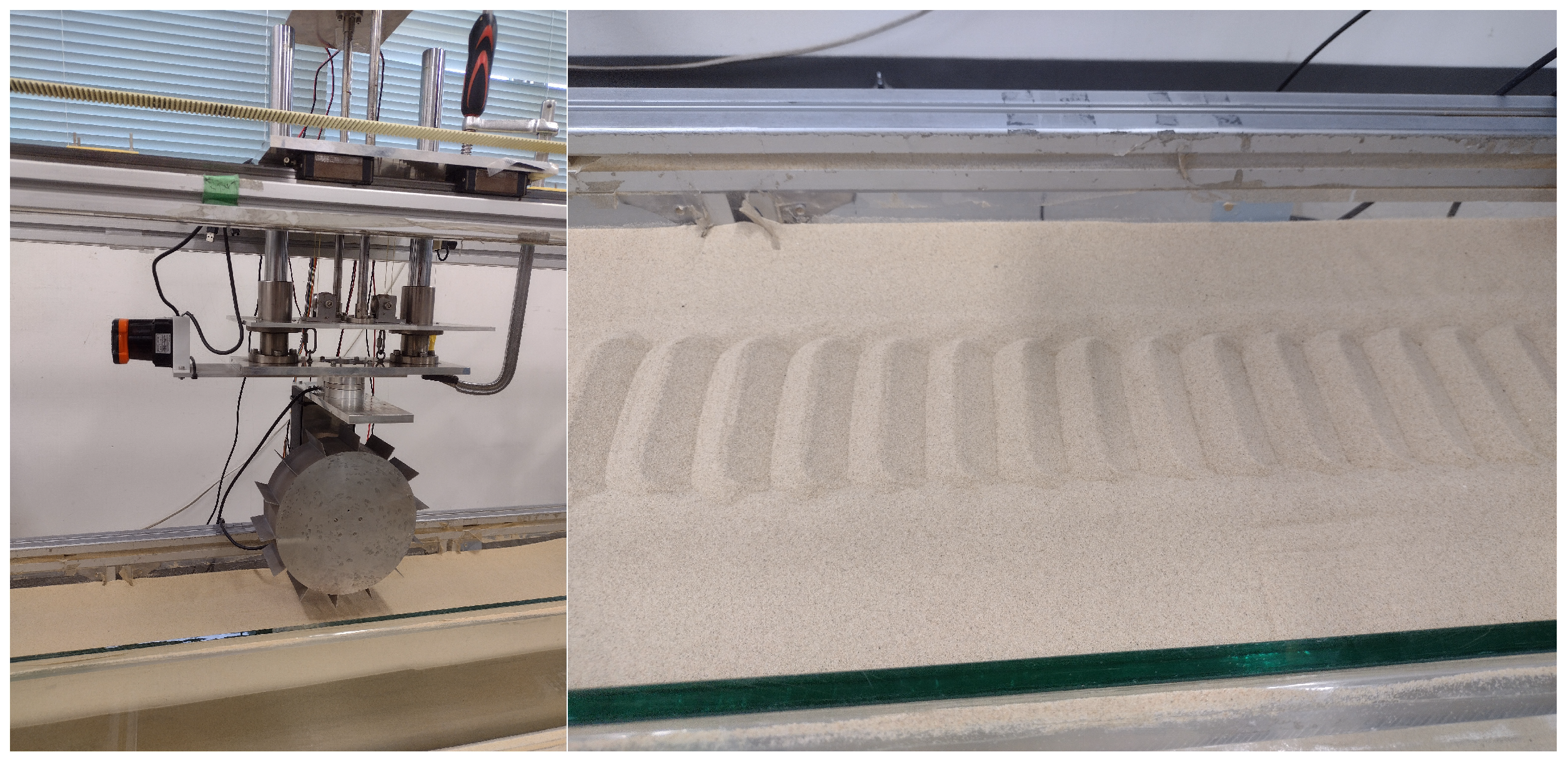
Figure 2.
Single-wheel testbed of Space Robotics Lab, Tohoku University [15].
Figure 2.
Single-wheel testbed of Space Robotics Lab, Tohoku University [15].
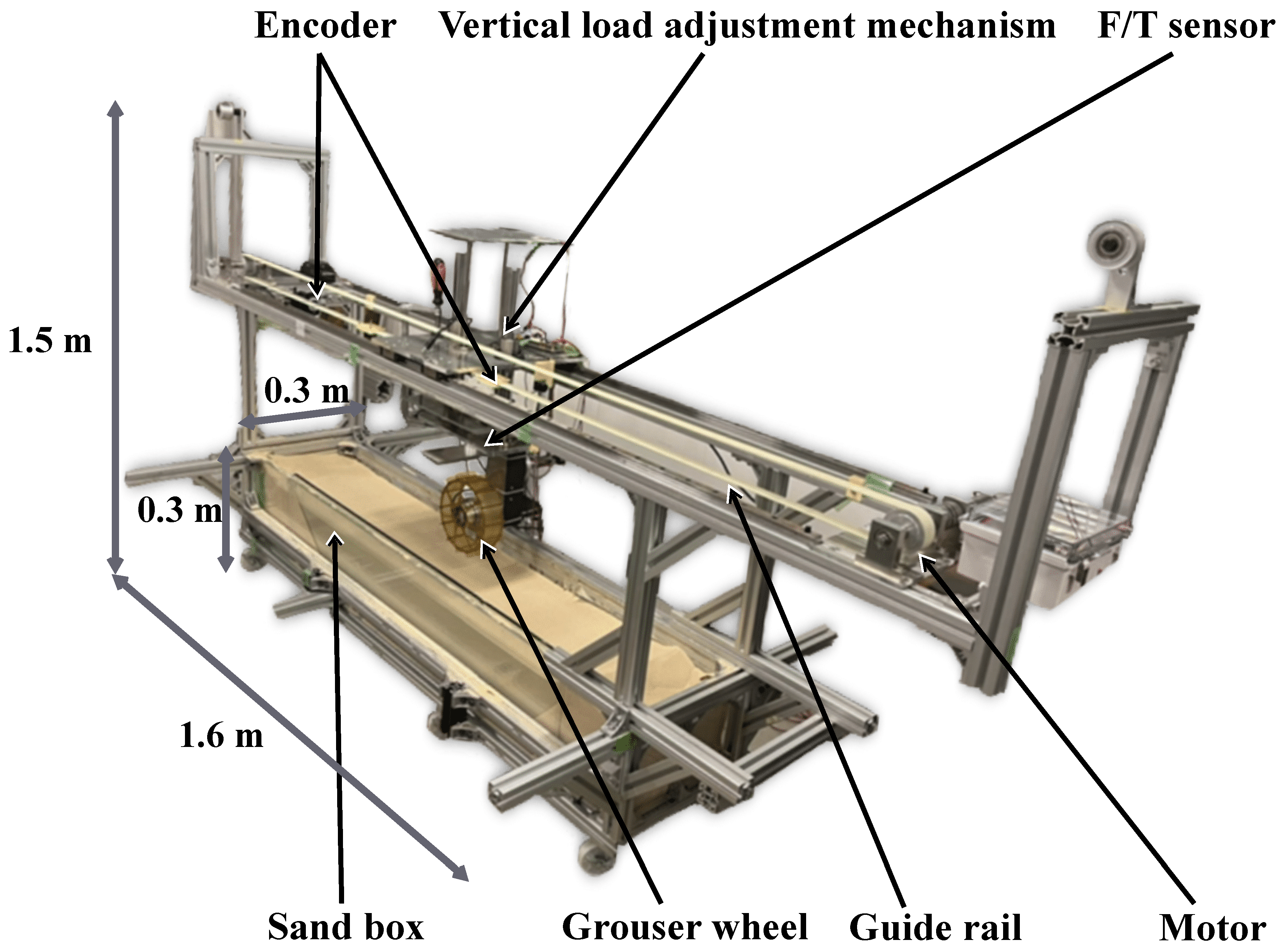
Figure 3.
Rashid rover and model of wheel, from UAE and Japan joint mission, used to create the ruts [15,18].
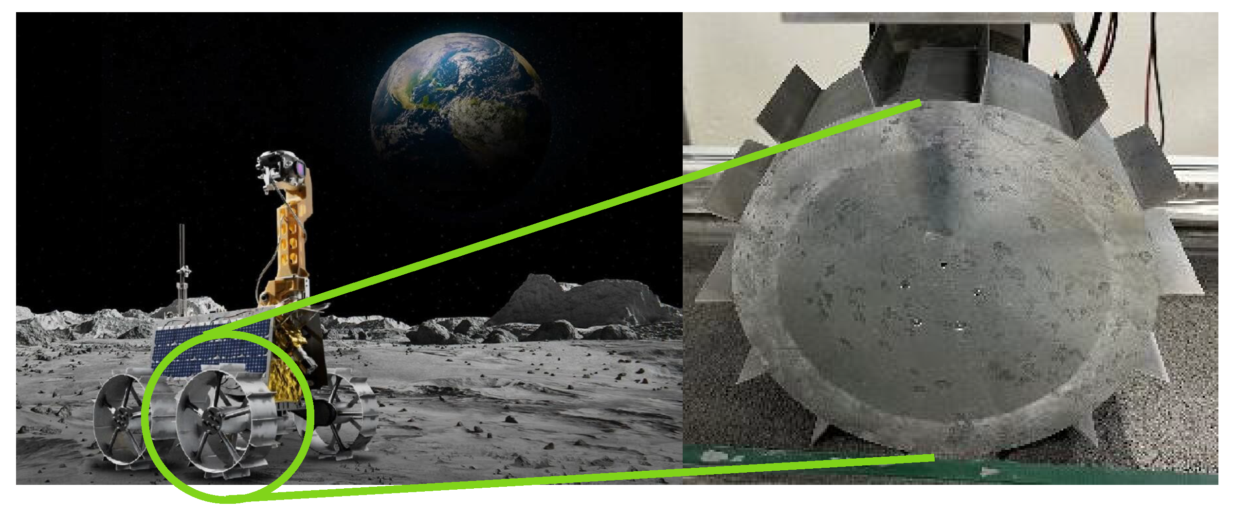
Figure 4.
Definition of heights and incline used in this paper.
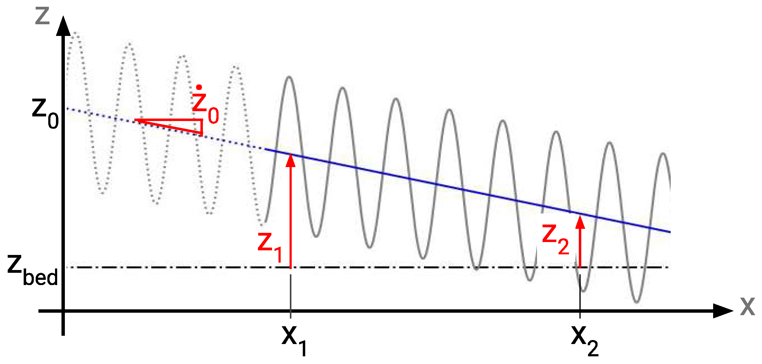
Figure 5.
Different values of moving average applied to LiDAR data.
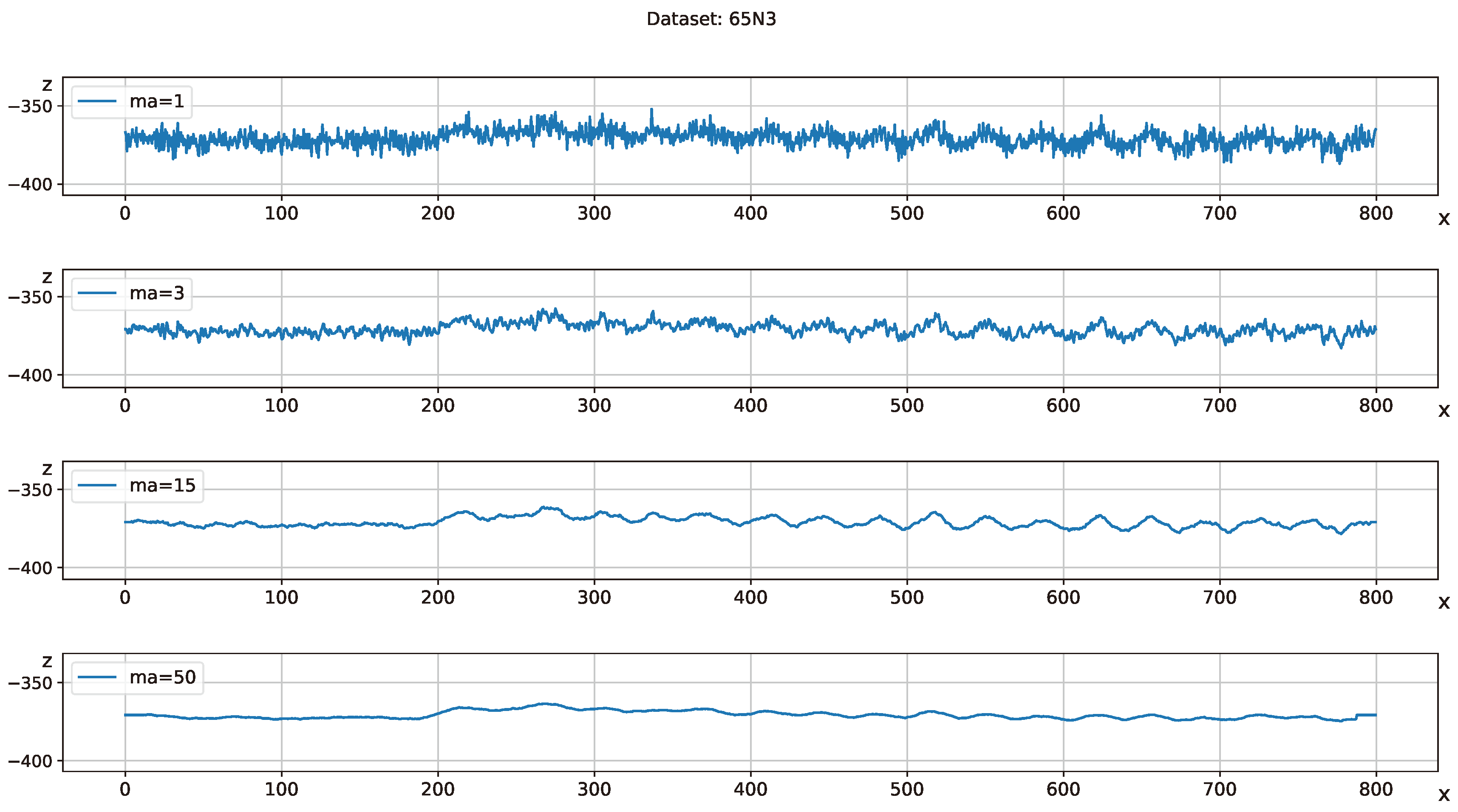
Figure 6.
Applying moving average (z_ma) with 15 data-points to 9 datasets.
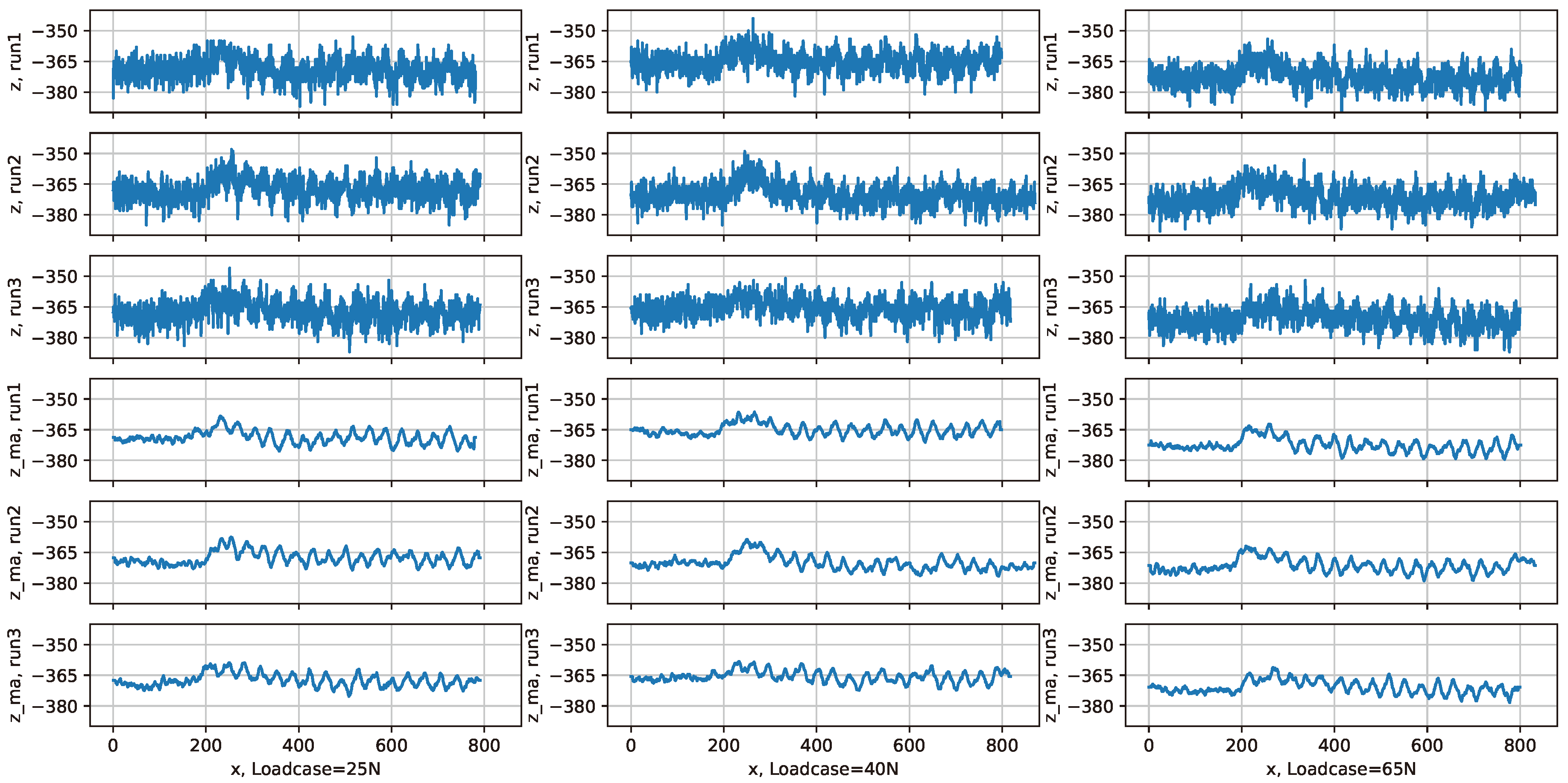
Figure 7.
Average of bed height in black and curve fit of sine wave in red. Dataset 25N1.
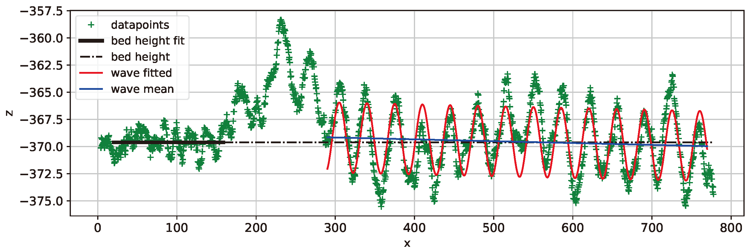
Figure 8.
Average of bed height in black and curve fit of sine wave in red. Dataset 25N2.
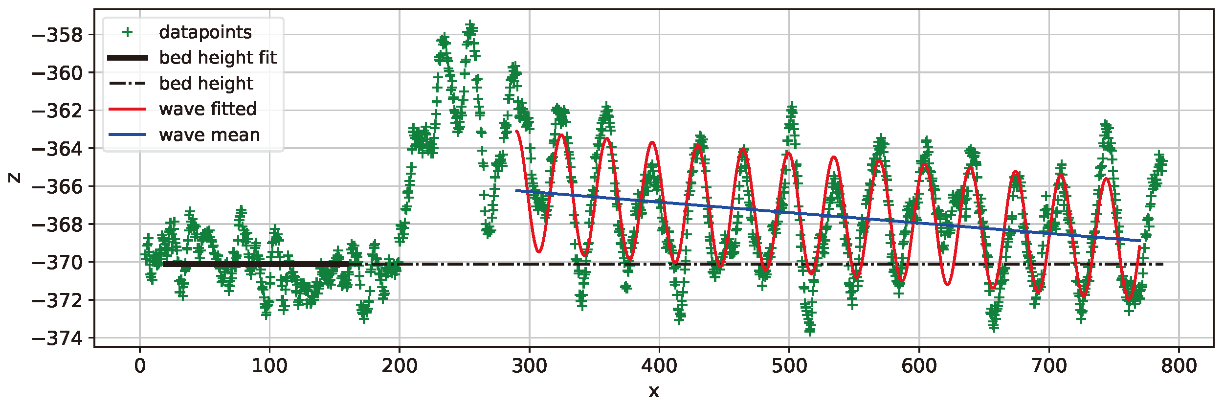
Figure 9.
Average of bed height in black and curve fit of sine wave in red. Dataset 25N3.
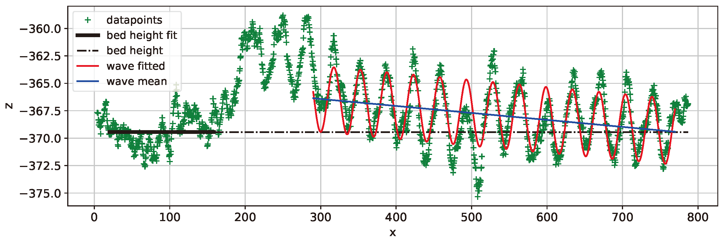
Figure 10.
Average of bed height in black and curve fit of sine wave in red. Dataset 40N1.
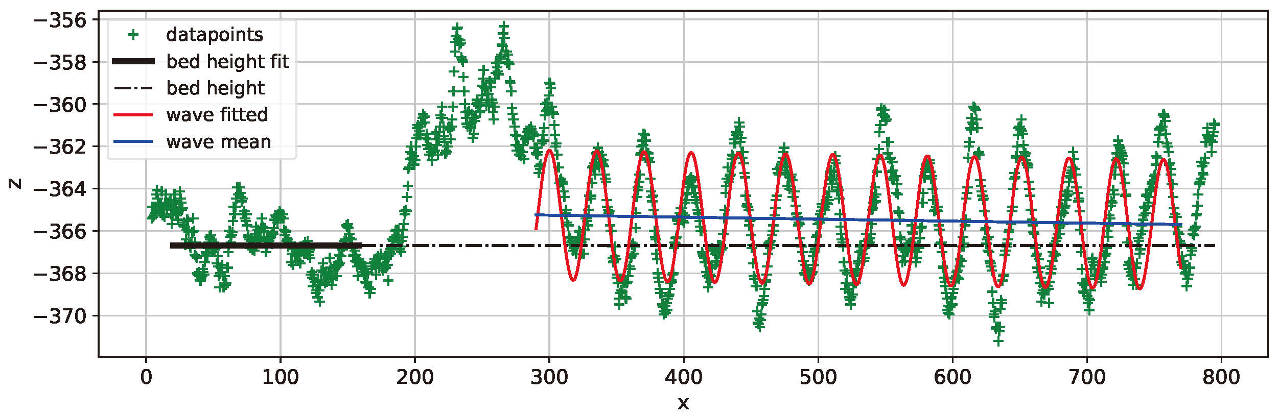
Figure 11.
Average of bed height in black and curve fit of sine wave in red. Dataset 40N2.
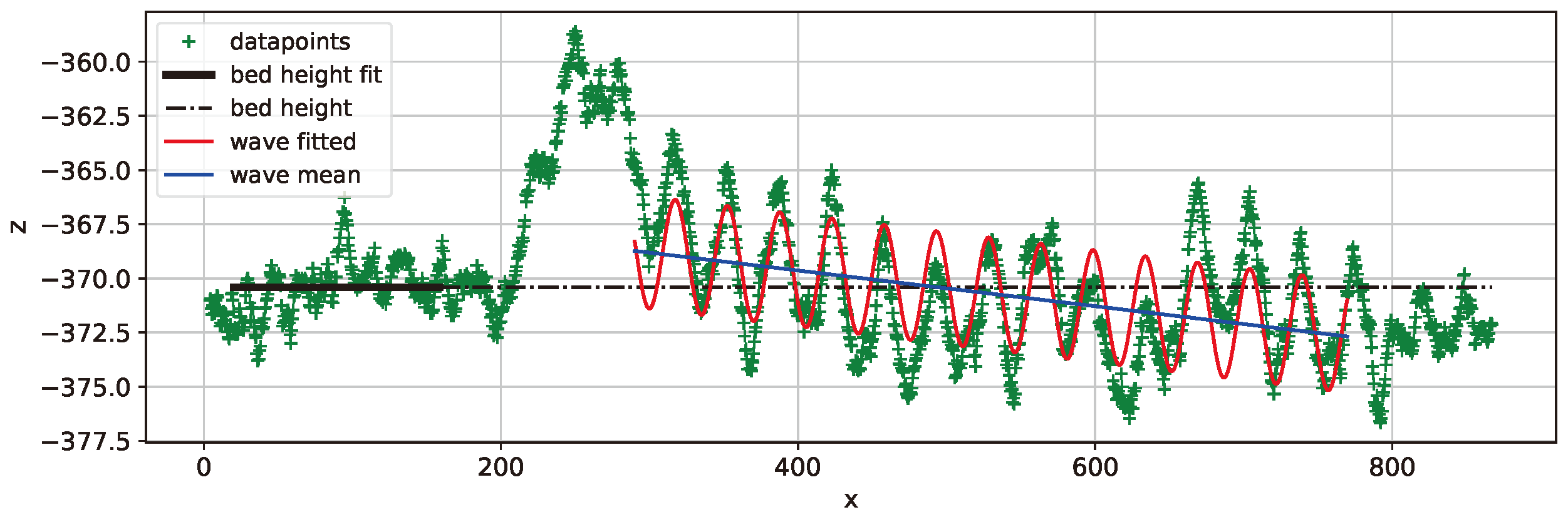
Figure 12.
Average of bed height in black and curve fit of sine wave in red. Dataset 40N3.
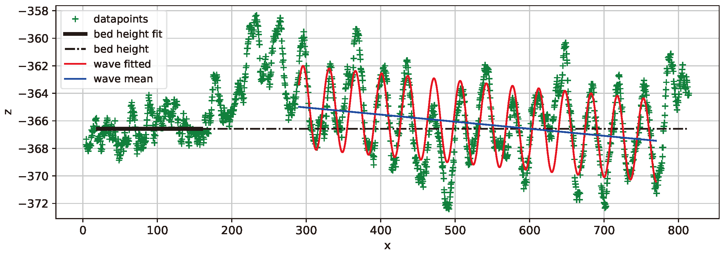
Figure 13.
Average of bed height in black and curve fit of sine wave in red. Dataset 65N1.
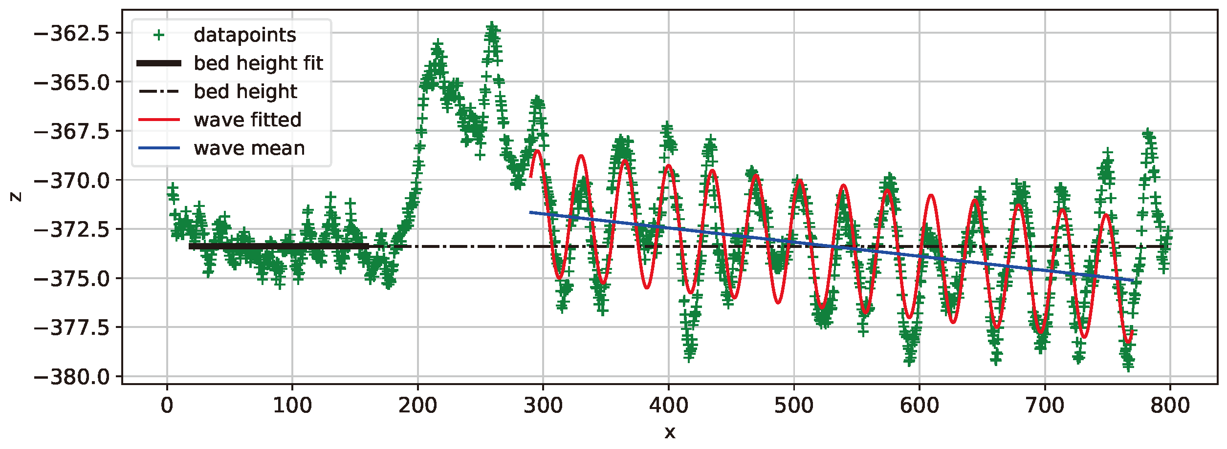
Figure 14.
Average of bed height in black and curve fit of sine wave in red. Dataset 65N2.
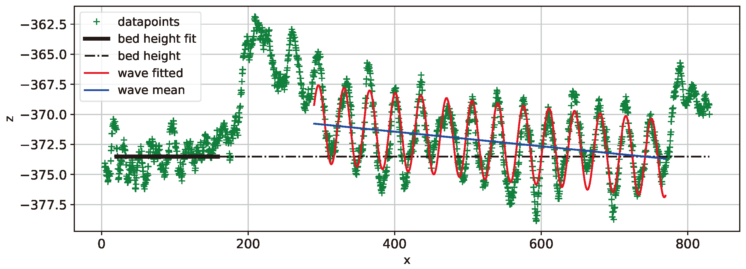
Figure 15.
Average of bed height in black and curve fit of sine wave in red. Dataset 65N3.
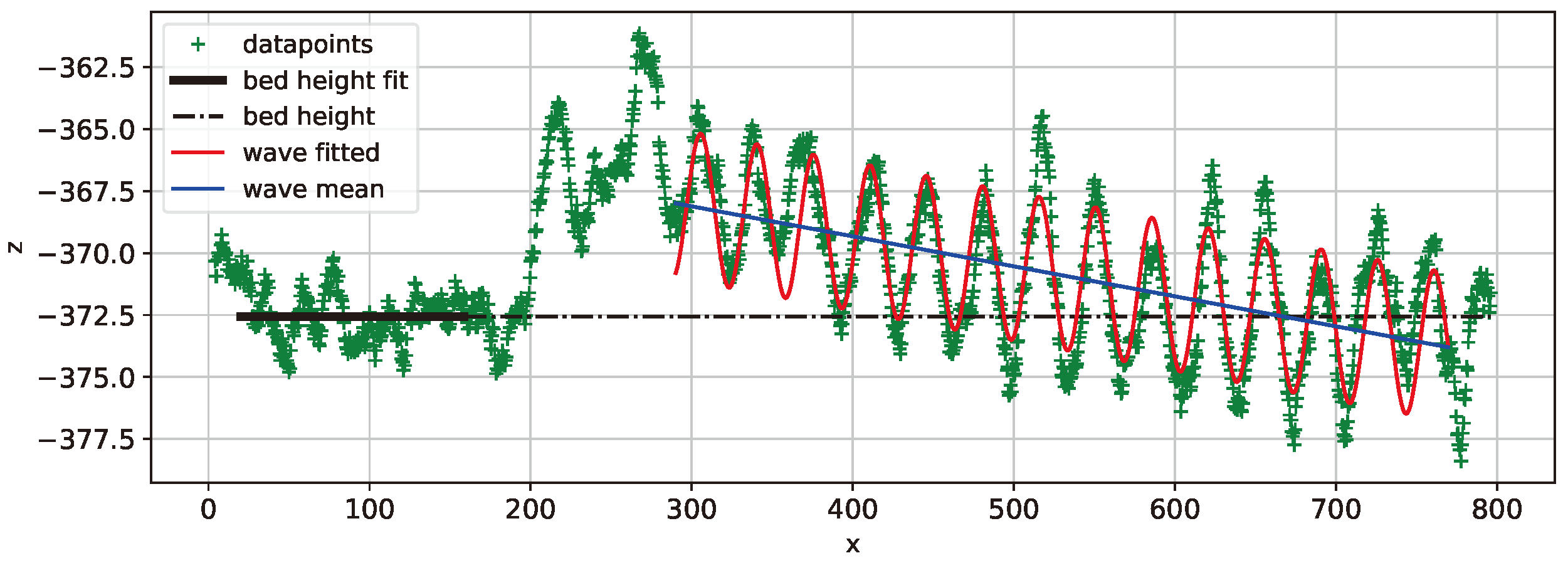
Figure 16.
Relevant parameters extracted: amplitude A, z_1, z_2, z_m, z_dif (). The points represent the average value per loadcase, and the error bars are used to show the lowest and highest values found in each testrun.
Figure 16.
Relevant parameters extracted: amplitude A, z_1, z_2, z_m, z_dif (). The points represent the average value per loadcase, and the error bars are used to show the lowest and highest values found in each testrun.
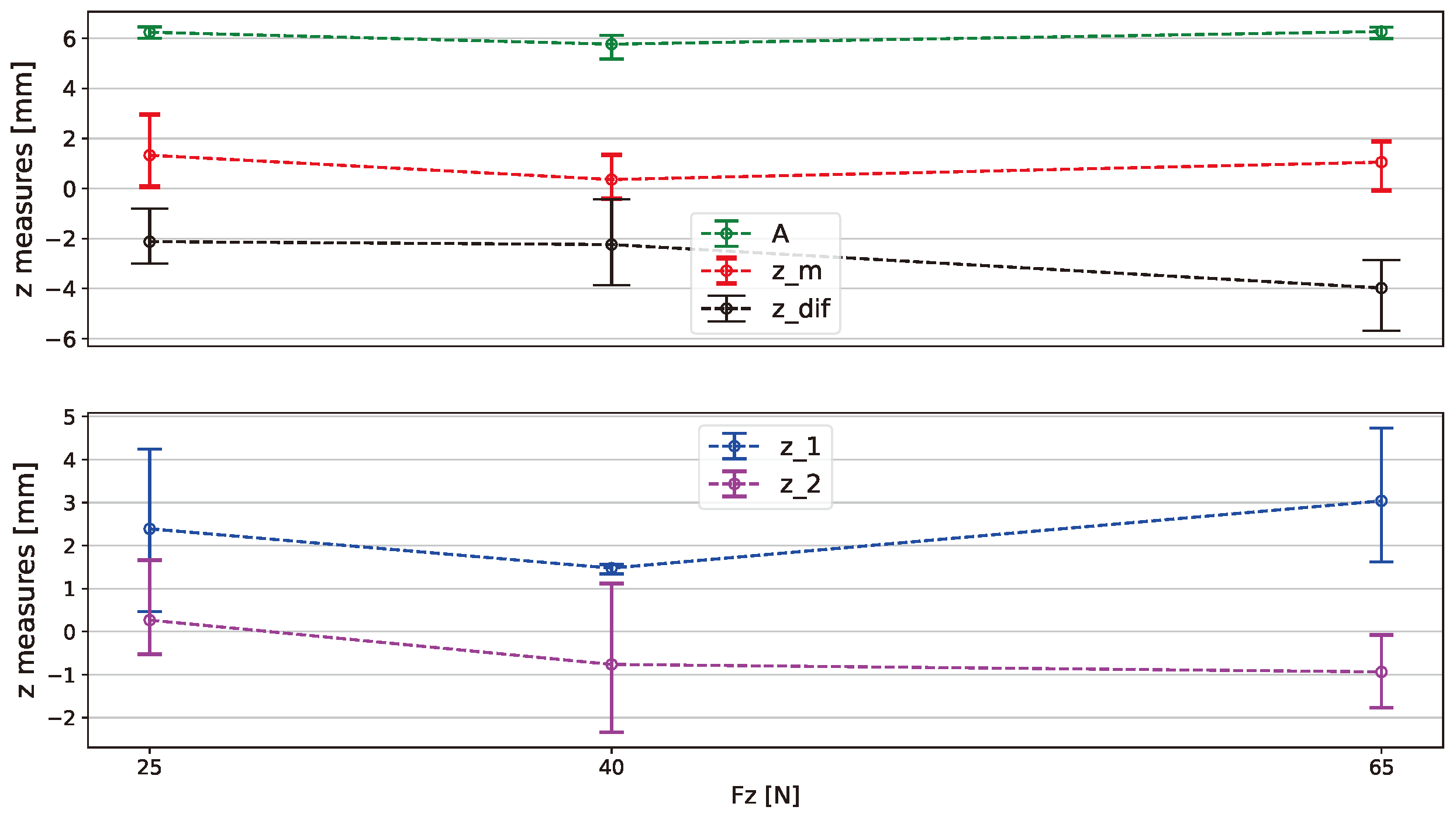
Table 1.
Mechanical properties of Toyoura Sand.
| Quantity | Value |
|---|---|
| Particle size () | 106-300 |
| Specific gravity () | 2.63 |
| Angle of repose (deg) | 36.0 |
| Friction angle (deg) | 38.0 |
| Cohesion (kPa) | 0.0 |
Table 2.
Bed Height selected intervals.
| Sample | Left limit | Right limit | Interval size | Bed Height |
|---|---|---|---|---|
| (mm) | (mm) | (mm) | (mm) | |
| 25N 1 | 20 | 159 | 140 | -369.62 |
| 25N 2 | 60 | 204 | 145 | -370.49 |
| 25N 3 | 0 | 175 | 176 | -369.15 |
| 40N 1 | 34 | 198 | 165 | -366.81 |
| 40N 2 | 38 | 198 | 161 | -370.26 |
| 40N 3 | 58 | 174 | 117 | -366.32 |
| 65N 1 | 0 | 199 | 200 | -373.28 |
| 65N 2 | 14 | 137 | 124 | -373.54 |
| 65N 3 | 35 | 198 | 164 | -372.73 |
Table 3.
Bed Height line fit error metrics.
| Sample | Mean Square | Mean | Maximum |
|---|---|---|---|
| Error (mm) | Error (mm) | Error (mm) | |
| 25N 1 | 0.91 | 0.79 | 2.44 |
| 25N 2 | 1.33 | 0.91 | 3.22 |
| 25N 3 | 2.23 | 1.19 | 4.02 |
| 40N 1 | 1.51 | 0.95 | 4.80 |
| 40N 2 | 1.12 | 0.78 | 3.99 |
| 40N 3 | 0.94 | 0.83 | 2.19 |
| 65N 1 | 0.97 | 0.80 | 3.15 |
| 65N 2 | 1.63 | 1.02 | 3.14 |
| 65N 3 | 0.87 | 0.76 | 2.53 |
Table 5.
Sine Fit Extracted Parameters. (: intercept, : incline, A: amplitude, : phase, T: period).
| Sample | (mm) | (mm/mm) | A (mm) | (mm) | T (mm) |
|---|---|---|---|---|---|
| 25N 1 | -368.67 | -0.00169 | 6.457 | 21.36 | 35.02 |
| 25N 2 | -364.64 | -0.00551 | 6.272 | -1.47 | 34.94 |
| 25N 3 | -364.52 | -0.00636 | 5.998 | 8.20 | 35.12 |
| 40N 1 | -364.97 | -0.00094 | 6.123 | 28.00 | 35.13 |
| 40N 2 | -366.34 | -0.00824 | 5.170 | 8.78 | 35.15 |
| 40N 3 | -363.49 | -0.00513 | 6.004 | 33.36 | 35.17 |
| 65N 1 | -369.57 | -0.00720 | 6.371 | 30.84 | 34.87 |
| 65N 2 | -369.01 | -0.00607 | 6.452 | 30.86 | 34.95 |
| 65N 3 | -364.49 | -0.01210 | 5.990 | 20.70 | 35.02 |
Table 6.
Sine fit error metrics.
| Sample | Mean Square | Mean | Maximum |
|---|---|---|---|
| Error (mm) | Error (mm) | Error (mm) | |
| 25N 1 | 2.86 | 1.40 | 4.16 |
| 25N 2 | 2.20 | 1.20 | 4.38 |
| 25N 3 | 2.14 | 1.16 | 4.91 |
| 40N 1 | 1.64 | 1.04 | 3.63 |
| 40N 2 | 3.32 | 1.53 | 5.02 |
| 40N 3 | 2.65 | 1.30 | 4.72 |
| 65N 1 | 1.81 | 1.12 | 3.41 |
| 65N 2 | 1.60 | 1.04 | 3.61 |
| 65N 3 | 1.90 | 1.09 | 4.67 |
Table 7.
Sine fit with relative height. A: amplitude, : phase, T: period, : z at beginning of wave, : z at end of wave.
Table 7.
Sine fit with relative height. A: amplitude, : phase, T: period, : z at beginning of wave, : z at end of wave.
| Sample | A (mm) | (mm) | T (mm) | (mm) | (mm) |
|---|---|---|---|---|---|
| 25N 1 | 6.457 | 21.36 | 35.02 | 0.47 | -0.33 |
| 25N 2 | 6.272 | -1.47 | 34.94 | 4.24 | 1.66 |
| 25N 3 | 5.998 | 8.20 | 35.12 | 2.46 | -0.53 |
| 40N 1 | 6.123 | 28.00 | 35.13 | 1.56 | 1.12 |
| 40N 2 | 5.170 | 8.78 | 35.15 | 1.53 | -2.34 |
| 40N 3 | 6.004 | 33.36 | 35.17 | 1.34 | -1.07 |
| 65N 1 | 6.371 | 30.84 | 34.87 | 1.62 | -1.77 |
| 65N 2 | 6.452 | 30.86 | 34.95 | 2.77 | -0.08 |
| 65N 3 | 5.990 | 20.70 | 35.02 | 4.73 | -0.96 |
Disclaimer/Publisher’s Note: The statements, opinions and data contained in all publications are solely those of the individual author(s) and contributor(s) and not of MDPI and/or the editor(s). MDPI and/or the editor(s) disclaim responsibility for any injury to people or property resulting from any ideas, methods, instructions or products referred to in the content. |
© 2024 by the authors. Licensee MDPI, Basel, Switzerland. This article is an open access article distributed under the terms and conditions of the Creative Commons Attribution (CC BY) license (http://creativecommons.org/licenses/by/4.0/).
Copyright: This open access article is published under a Creative Commons CC BY 4.0 license, which permit the free download, distribution, and reuse, provided that the author and preprint are cited in any reuse.


