
Submitted:
03 June 2023
Posted:
05 June 2023
You are already at the latest version
Abstract
In this study, UAV (Unmanned Aerial Vehicle) photogrammetry was used to monitor the ground displacement on the slope below a coal waste-rock stockyard, and to investigate the role of rainfall on this displacement. The study area is a mountainous region in Korea, where coal mining continues, and coal waste-rock is stored on the slopes of the mountain. In this area, ma-terial removal work was undertaken to reduce the steepness of the slope and driving forces in order to prevent disasters, but the strategy requires continuous monitoring to confirm the stabilization of the slope. For slope monitoring, a total of six UAV photogrammetry campaigns were conducted between April 2019 and August 2020. As a result of data processing, an orthoimage and DSM (Digital Surface Model) were generated. The ground displacement was estimated through four ways: slope extraction, displacement area evaluation, horizontal displacement, and vertical displacement analysis. During the study period, the maximum vertical displacement was 3.3 m and the maxi-mum horizontal displacement was 3.5 m. The horizontal displacement was effectively evaluated through the measurement of the movement of the drainage system using orthoimages that captured with a periodic survey. The effects of rainfall on ground displacement were also investigated. A very clear linear relationship between rainfall intensity higher than 20mm/d and ground displacement was identified. Accumulated amount of rainfall also showed good correlation with slope movement, but the frequency of rainfall intensity below 20 mm/d showed relatively low correlation with ground dis-placements.
Keywords:
Slope displacement
; UAV
; DSM
; Rainfall intensity
1. Introduction
Steep hills constitute about 64% of the total area of South Korea. These hills have a high distribution ratio of weathered granite masses with low cohesive strength, increasing the risk of disasters such as landslides and debris flows. Large-scale mountain soil and sediment erosion occurred during Typhoon Rusa in 2002 and Typhoon Maemi in 2003, resulting in landslides and debris flows [1,2]. The Erosion Control Work Act of South Korea has been in charge of the designation of areas prone to landslides and debris flow since 2011 and established a control system to prevent them. However, measures for soil creep are still not in place due to underreported cases and a lack of studies and techniques to manage them [3,4,5]. Soil creep has been found in about 35 locations in Korea and this is expected to increase as more are being identified [6]. However, due to the presence of large clods of soil covering these areas and the very slow nature of soil creep, accurately monitoring and predicting hazardous conditions are challenging [7,8].
There are numerous different methods and approaches to identify ground de-formation by analyzing the characteristics of areas prone to soil creep. Remote sensing methods have been used for the monitoring of ground deformation or landslides. Optical remote sensing images offer detection of horizontal displacement in wide areas [9,10]. Many applications concerning landslide monitoring have been conducted by remote sening techniques such as InSAR (Interferometric Synthetic Aperture Radar) [11,12,13,14,15,16,17]. Global Navigation Satellite System (GNSS) enables low-cost and efficient landslide monitoring [18,19,20,21]. Terrestrial laser scanning (TLS) provides 3-D information with high density point cloud data and can generate DSM (Digital Surface Model) having very high resolution [22,23,24,25]. Some commonly used research methods include the assessment of risks by recording the locations where a mass movement occurred and building a database of activity [26,27], numerical modelling for the prediction of the range and impulse of the landslide and debris flow by using a dynamic model [28,29,30], and experiments reproducing the actual phenomena [31]; all these which can be enhanced by information gathered through remote sensing techniques.
High-resolution topographic data obtained by a UAV (Unmanned Aerial Vehicle) photogrammetry is verified by using various methods such as a comparison with satellite images, confirmation through the generation of digital topographic maps and inspection (e.g. ground control points). UAV can further be deployed using a low-cost camera to capture the area of interest, and comparing the accuracies obtained from fixed-wing and rotary-wing UAVs with given minimum requirements for the geohazard being analyzed, therefore decreasing monitoring costs [32]. Recent technological advances allowed researchers to obtain data from hard-to-reach areas, resulting in utilizing UAV in mountainous regions and regions with mass movements in a safe manner and with enhanced detail [33]. Importantly, topographical changes in landslides can detect complex displacement patterns using subsequent DTMs (Digital Terrain Model) [34]. Other researchers have used the technique to calculate surface displacements caused by mining activities and earthquakes, which can be effectively monitored using UAVs [35,36]. Even when the ground collapses, this technique has been used to monitor ongoing, post-collapse surface displacements [37].
Time series of DTMs, and particularly point clouds derived from LiDAR or photogrammetry can be used for Change Detection. This technique compares the distance between point clouds in the normal direction to the surfaces in a statistical manner [38]. This technique provides useful information, how-ever slope displacements can be far from perpendicular to the slope surface, and other complementary techniques could aid in interpreting the true slope dis-placement vectors.
This research describes the possibilities for using UAV photogrammetry and techniques that could be used as complementary to Change Detection, to monitor slope deformations. The approaches are illustrated for a slope with coal waste-rock stockyard. The slope of the study area is adjacent to a residential area, and landslides are occurring continuously with a possibility of damage to the public from large-scale landslides. To prevent large-scale damage, investigations using sensors have been conducted previously, but UAV is considered a very appropriate alternative as a cost-effective monitoring method. One methodology proposed here determines vertical and horizontal terrain displacements without any additional sensors.
It has been well documented that rainfall can trigger shear deformation of slopes mainly through infiltration [39,40]. Some investigations in the subsidence area indicate that rainfall is a determinant of severe subsidence [41,42,43]. The time variation of shear deformation is essential for risk assessments, and slope deformation needs to be monitored appropriately. In previous studies, ground displacements due to rainfall was monitored using sensors, but the survey through the sensor only proved ground deformation at a discrete location. In this study, the effect of rainfall characteristics such as intensity and cumulative rain-fall on ground displacement is quantitatively investigated. If the effect of rainfall on landslides is clearly investigated, it can be used as an important factor for early warning of landslides, and is a consideration in the installation of structures in preparation for landslides.
2. Materials and Methods
Figure 1 shows the flow chart for this research. An essential part of this study is the estimation of ground displacements and the investigation of the effect of rain-fall on ground deformation. UAV photogrammetry and geographic information system (GIS) were effectively used to estimate the ground displacements. The UAV used was a DJI's Phantom 4 pro, and the aerial surveyed source data were post-processed through the Pix-4D program. The data acquisition step also establishes a UAV flight plan for obtaining point cloud data, a set of data points in space that produces a digital elevation model (DEM) or a digital surface model (DSM). As GPS sensors become increasingly unreliable due to UAV instability, UAV speed, and wind; the site was surveyed to compensate for errors in the sur-vey data and ground control points (GCP) were surveyed, that included the entire study location. The photogrammetry data were obtained from April 3, 2019, to August 14, 2020, using the UAV to analyze the topographic changes at the re-search location. Comparisons between the 3D topographic data sets during 16 months, including the rainy season obtained by the UAV, were possible with these datasets.
Data collection would be more effective if the research location is within range of the GCPs. 6-9 GCPs were installed in the study area (Table 2). After obtaining the GCP data, preparations for aerial photogrammetry were made, including flight altitude, flight time, range, camera resolution, and image overlay. Orthoimages and DSM are generated as the result of post-processing, and the ground displacement was estimated using these data. Displacement analysis consists of four types: slope extraction, displacement area evaluation, horizontal displacement, and vertical displacement analysis. Orthoimages were used for horizontal displacement analysis, and the drainage system installed on the slope for surface water outflow was used as a reference for horizontal displacement analysis. The drainage system on the slope is easy to identify by UAV photogrammetry, and since it is installed at a regular distance, the displacement of the entire area of the slope can be measured. This method provides high accuracy of horizontal displacement. DSM is used to analyze the amount of vertical dis-placements. Based on the DSM generated for each period, the amount of vertical displacement is determined by analyzing the surface elevation change to the pre-set baseline surface. Several baselines were used to show the most representative cross-section in the study area. The effects of rainfall on ground displacement were investigated using daily rainfall intensity and cumulative rainfall. The daily rainfall intensity was evaluated by dividing it into rainfall higher than 20mm/d and rainfall lower than 20mm/d. The effect of rainfall on ground deformation was then quantitatively evaluated.
3. Study Area and Field Surveys
The research area is located in Samcheok city, Kangwon Province, Korea. The geographical coordinates are 129°2'40'' east longitude and 37°13'20'' north latitude (Figure 2). The surface geology of the slope, in which the research area is located, corresponds to the Early Triassic Pyeongan Supergroup, and the main layer has a thickness of about 150 to 250 m, where milky white coarse-grained sand-stone and coarse sandstone dominate, and dark gray sandstone and shale are included.
Because of possible slope hazards, researchers conducted safety investigations and location reviews in the past. These show that the area's altitude has increased from 20 m to 49 m due to placement of the coal waste dump [44]. Slope stabilization was attempted after the collapse of a small portion of the slope in the past. Blocking and cascade drains were installed, however, ground deformation at this location was still prevalent, causing tension cracks, loss of topsoil, and dislocation of drainpipes, leading to a massive collapse of the slope. The Coal waste storage is located 150m above the research site. The load imposed by this stock pile was expected to be the cause of the ground displacement. The ground is compressed by the load and pushes the slope as it moves downwards. The angle of the coal waste deposit is 34°, the distance between the bottom of the deposit and the top is approximately 70 m, and the horizontal ex-tent is approximately 120 m. A cut slope below the coal waste deposit had a width of 100 m, an angle of 26°, and a surface area of 7,000 m2. A sudden mass movement can cause massive damage to residential areas below the study site if the slope collapse.
Two types of equipment were used to survey the research area. Figure 3A shows a set of equipment used to measure the GCPs composed of an RTK receiver and a controller pole. It received approximately 30 satellite signals, using 25 for RTK positioning. The accuracy of the RTK is 8 mm horizontally and 15 mm vertically, with the maximum root mean square deviation (RMSE) of 15 mm. Figure 3B shows the remote-controlled UAV with a camera used for topographic surveys. The data obtained from photographic images were used for spatial analysis. The UAV weighs 1.4 kg, has a maximum flight altitude of 6,000 m, a maximum speed of 72 km/h, a maximum range of 7 km from the controller, and a maximum flight time of 30 minutes.
Between April 3, 2019, and August 14, 2020, a total of 6 UAV photogrammetric surveys were conducted on the study area (Figure 4). The red dot represents the points where photos were taken during the flight path. Atmospheric conditions for each flight were different, and flight conditions were set differently accordingly. Moreover, if necessary, the survey area was set differently (Table 1).
Surveying the GCPs was necessary to generate coordinates for the photographic data obtained by the UAV. The GCPs are the reference points surveyed directly from the research location, and they serve as the reference for the horizontal location (X, Y) and height (Z) of the cut slope. The GCPs were selected based on the road around the cut slope and the corner of the drainage (Figure 5) to accurately identify the location of the reference points. The number and location of GCPs in each period were adjusted according to the conditions of the investigation.
The conditions and Root-Mean Square Error (RMSE) of each GCP obtained at each period are summarized and shown in Table 2. If the survey area is large, more GCPs are required, and we tried to use the same GCP location as much as possible.
The RMSE values of April 3, 2019, were 0.034 m, 0.015 m, and 0.044 m in the X, Y, and Z directions, respectively, and the average RMSE is 0.031. In comparison, the RMSE values of October 13, 2019, were 0.032 m, 0.027 m, and 0.032 m in the X, Y, and Z directions, respectively, and the average RMSE is 0.030. At each ground point of the survey, the RMSE of the GCP was considered to satisfy the accuracy.
Through UAV photogrammetry and 3D data construction, orthoimages and DSMs of each period were generated (Figure 6). In the figure, the colour of the line is displayed differently depending on the time of the survey. The resolutions of the generated othoimages were less than 2 cm. The total number of surveys was six times, including two rainy seasons, and it was considered sufficient to investigate ground displacement. In some cases, a tarp was temporarily installed in the study area, but it did not interfere with the study's progress.

Table 2.
RMSE of GCPs.
| April 3, 2019 | October 13, 2019 | December 22, 2019 | April 10, 2020 | July 16, 2020 | August 14, 2020 | |
| N. of GCP | 9 | 8 | 7 | 9 | 9 | 6 |
| N. of Photos | 305 | 104 | 213 | 395 | 477 | 278 |
| Overlap rate (%) | 90 | 80 | 87 | 87 | 90 | 90 |
| X-RMSE (m) | 0.034 | 0.032 | 0.034 | 0.040 | 0.020 | 0.019 |
| Y-RMSE (m) | 0.015 | 0.027 | 0.014 | 0.035 | 0.029 | 0.035 |
| Z-RMSE (m) | 0.044 | 0.032 | 0.008 | 0.029 | 0.035 | 0.038 |
| Mean Error (m) | 0.031 | 0.025 | 0.011 | 0.034 | 0.028 | 0.028 |
4. Results and Discussions
Terrain changes for 16 months from April 2019 to August 2020 were analyzed using orthoimages and DSM, which were generated by UAV photogrammetry. Only the cut slopes were extracted from the images and used for the time-series analysis of ground displacement, and the extracted DSM shows the change of the fully exposed surface well. The surface of the slope and the drainage system were revealed in the orthoimage, and the drainage system on the slope has been used as the baseline for the ground displacement analysis.
The first step in the ground displacement study would be to confirm the hazardous area that may cause the displacement. The area of ground displacement may change with time, and in particular, may change depending on the frequency and intensity of rainfall. The area of the ground displacement and the intensity of the deformation becomes essential data for the decision of the countermeasures for managing the risks associated with this slope.
Figure 7 shows the map of vertical displacement, or topographical change, from April 2019 to August 2020. The difference was calculated by subtracting the DSM of each period as of April 2019. The results of the analyses were shown in blue-red gradation; blue and red indicate the rise and subsidence of the ground, respectively. As the time series analysis results, it can be seen that the ground displacement area does not change significantly over time and remains constant. These results indicate two points about the ground displacement of the slope of the study area: One is that the cause of the ground displacement appears to be due to the rise of groundwater due to rainfall, not a load of the waste coal on the upper slope (see Figure 2). If it is due to the load on the top of the slope, the displacement range is expected to occur over the entire slope, particularly close to the location of the coal stockpile. Another is that the constant pattern of the ground displacement implies that the horizontal mass movement is the dominant status on the slope.
Following the area analysis, ground displacement over six months were analysed using the orthoimage and DSM. For the analysis, it was necessary to set the baseline, and Figure 8 shows the seven baseline positions for the analysis. In Figure 8, the highest position of the slope is in the vicinity of ① and ③, and the surface flow is in the direction of ① and ②. A drainage system is installed for surface drainage, and its location is consistent with No. ③, ④, ⑤, ⑥, and there is ⑦ on a retaining wall at the lower part of the slope. Figure 8B shows the distribution of uplift and subsidence as a result of displacement. For clear visualization, vertical displacement less than 0.1 m is not shown.
Figure 9 shows the profile of elevation change over 16 months from April 2019 to August 2020 at baseline ①. The small figure in Figure 9 shows the change more clearly over the 10-40 m distance. Baseline ① shows the longitudinal change of the slope, and it can be seen that the change is continuously progressing within the investigation period. In particular, it shows that the ground dis-placement is predominantly horizontal.
Figure 10 shows the change in elevation by subtracting the surface elevation at each period from the surface elevation in April 2019 at the baseline ①. In the figure, the red line corresponding to the 0 value on the y-axis represents the ground elevation in April 2019, which means the ground elevation before the occurrence of ground displacement. Moreover, based on this ground elevation, the change of ground displacement for each period is shown. A value of 0 on the x-axis indicating the distance indicates the lower part of the slope, and the distance increases as it goes to the upper part of the slope. The elevation change is not constant and is thought to be due to the influence of the drainage system on the slope. As the horizontal drainage system moves laterally, the net change in-creases significantly or results in close to zero.
In Figure 10, the ground displacement is shown to increase, and if such continuous ground displacement is accumulated, it is expected that a large-scale land-slide collapse could occur in the future. Ground displacement occurring at the landslide site is mainly caused by collapse, erosion, and deposition. However, the ground subsidence at the top of the slope is relatively small, results would apparently show that the slope experienced an uplift process. It can be seen that this apparent uplift is zero at the x-axis distance of 25m and 53m. As shown in Figure 9, there is a horizontal (flat) area with drainage channels in these locations. These results show that the ground displacement is caused by horizontal movement rather than vertical change, with the horizontal displacement leading to that apparent but misleading uplift. In addition, it can be seen that the displacement is more significant in the region where the distance is close to 0, and this is expected to be the result of accumulated displacement at the lower part of the slope. It was found that the change was larger at the lower part of the slope, and that soil arches also occurred. In addition, it can be seen that the change in each period is very different. The ground displacement is expected to be related to rainfall, and further investigation is needed.
Figure 11 shows the elevation change during the period as shown in Figure 9 at the baseline ②, and the change is more clearly expressed in the distance of 45-60 m. Baseline ② is also constantly changing, but it can be seen that the change is small compared to baseline ①. In particular, the change in topography from April 2019 to August 2020 shows that the ground subsided. Unlike the horizontal dis-placement shown in Baseline ① in Figure 9, the displacement in Baseline ② appears to be due to ground subsidence. These results show that the displacement of the slope can be caused by a combination of horizontal displacement and subsidence for certain locations.
This trend is well shown in Figure 12 and shows that ground subsidence occurs at the slope's upper side. In Figure 10, the elevation change represents a waveform assuming a typical shape of elevation change caused by horizontal displacement. The elevation change pattern in baseline ② has a different shape from baseline ①. The subsidence of the upper slope and the rising of the upper slope are typical features of ground movement that has a rotational component in its kinematics. In particular, the section where the ground subsidence is a section where groundwater infiltration is active, and a countermeasure method to remove groundwater or prevent surface water infiltration could be effective.
From these results, it was considered that the landslide was progressing while the ground displacement showed the characteristics of soil creep. Considering that rainfall was an important cause of such ground displacement, an analysis was conducted on the progress of ground displacement caused by rainfall. The baselines ③, ④, ⑤, and ⑥ in Figure 12 are for horizontal displacement analysis different from the baselines ① and ②. The horizontal displacement analysis process is shown in Figure 13. For the analysis, the moving direction and the moving distance were measured based on the drainage channel locations by overlapping the orthoimages of each period.
Figure 14 shows the analysis results of horizontal displacement. Distance 0 means the starting point of each baseline indicated by a circle in Figure 13. Figure 14A–D represent the baselines ③, ④, ⑤, and ⑥. In (D), the drainage system was demolished during the investigation period, making continuous analysis impossible. For the other baselines, five ground displacements were measured using orthoimages. It can be seen that the displacement at each baseline is different, and the displacement is larger as it goes to the lower part of the slope. Excluding the baseline ⑥, the displacement was the largest at the baseline ⑤, and the dis-placement was 3.5m for 16 months.
Figure 15 shows the deformation of the retaining wall installed at the lower section of the slope. Figure 15A shows that the retaining wall is installed in a straight line without any deformation, but Figure 15B shows that the retaining wall is significantly deformed after six months. Figure 15C is an overlapped orthoimage showing how far the retaining wall has been moved. The dotted line in Figure 15C was where the retaining wall was in April 2019, and the solid line was where the retaining wall was located in October 2019. The 27.5 m earth retaining wall was moved 3.0 m southwest from the 8 m section on the left. The baseline ⑤ and ⑥ showed the drainpipe’s horizontal (southwest) movement, confirming the occurrence of mass movement on the slope over six months. The drainpipe and the earth retaining wall of the cut slope indicate a slope failure, and the movement observed can be understood as soil creep.
The primary purpose of this study is to analyze the ground movement and the effect of rainfall on slope movement. Figure 16 shows the daily rainfall data collected during the study period from the weather station closest to the study area. Rainfall occurs intermittently during the study period, and it can be seen that rainfall of more than 20mm/d frequently occurs between July and October, which is the summer period. It can also be seen that strong rainfall of more than 150mm/d occurred during the study period. For analysis, rainfall over 20 mm/d was marked with a red circle. Ground collapse due to strong rainfall of more than 100mm/d is well known, but the effect of medium-intensity rainfall of about 50mm/d on the ground displacement needs additional investigation. Therefore, in this study, rather than an analysis based on cumulative rainfall, daily rainfall was used to examine the effect of rainfall intensity on ground displacement. ①-⑤ in the upper part of Figure 16 indicates the discontinuous UAV photogrammetry periods for the ground deformation monitoring. The 6 UAV photogrammetric surveys were divided into five representative time windows. Each of the five windows is shown by a bar of a different colour. A red circle indicates rainfall intensity exceeding 20mm/d, and rainfall not exceeding 20mm/d is indicated by a white circle.
Regression analysis results are shown in Figure 17 using rainfall data and the ground displacement data. In Figure 17A, the x-axis represents the number of times a rainfall intensity during the rainfall that occurred during the analysis of the topography change of the five sections (above or below the 20 mm/d thresh-old). The y-axis represents the amount of ground displacement using the result of (C) among the ground displacements shown in Figure 14. The result of (C) was used because it was considered that the baseline ⑤ was located at the lower section of the slope and could adequately represent the ground displacement. For better understanding, different colour of each symbol is arranged corresponding to the colour of each period in Figure 16. The circle in Figure 17A represents the displacement caused by the rainfall intensity exceeding 20mm/d, and the square represents the displacement caused by the rainfall intensity less than 20mm/d. If the rainfall intensity is expressed separately, the influence of high or low rainfall intensity on the ground displacement can be investigated. The rainfall intensity and the ground displacement showed a linear relationship. Although the number of times of each rainfall intensity and displacement showed a linear relationship, the R-squared value showed a higher correlation with high rainfall intensity. In Figure 17B, the effect of accumulated amount of rainfall on ground displacement was also investigated and showed a clear linear relationship to the ground dis-placement. These results show that the influence of rainfall is remarkable among the causes of displacement. It was thought that an appropriate drainage system for runoff of rainfall is essential for the stable management of slopes, and facilities for the exclusion of groundwater are also required. Furthermore, forecasting cumulative precipitation would allow forecasting landslide displacement with a significant accuracy, which can provide enhanced information for early warning systems.
5. Conclusions
In this study, UAV photogrammetry was adopted to monitor the ground dis-placement occurring on the slope below the coal waste-rock stockyard. The re-search area has applied slope stabilization and drainage system for surface water outflow after the collapse of the slope in the past. However, even the slope stabilization, the ground deformation of the cut part was still prevalent, resulting in a large-scale collapse of the slope, such as tensile cracks, loss of topsoil, and drainage pipes. In past studies, monitoring surveys using sensors have been con-ducted in this area, but more intensive investigations are needed. Six UAV photogrammetry was conducted between April 2019 and August 2020, and the ground displacement on the slope below the coal waste-rock stockyard was con-firmed. Orthoimages and DSM generated through post-processing provide a quantitative assessment of horizontal and vertical displacement on slope. Based on the DSM for each period, vertical displacement was evaluated through the surface elevation change in the preset baseline, and the maximum vertical dis-placement was 3.3 m during the study period. The horizontal displacement was evaluated through the measurement of the movement of the drainage system using orthoimages captured with a periodic survey, and the maximum horizontal displacement was 3.5 m during the study period. The effects of rainfall on ground displacement were also investigated with daily rainfall intensity, dividing it into higher than 20mm/d and lower than 20mm/d and accumulated amount of rainfall. Higher rainfall intensity over 20mm/d and accumulated rainfall showed a clear linear relationship with horizontal displacement. This study confirmed the effect of rainfall on the ground displacement. These results imply that proper drainage of the surface runoff water and groundwater discharging is important in deter-mining a slope stabilization method. The UAV photogrammetry was very effective for monitoring ground displacement because it could extract moving area and assess the vertical and horizontal displacement with high precision. Further-more, this study presented displacement measurement approaches for estimating horizontal and vertical deformation using point clouds and DSMs that would complement deformation information as obtained from Change Detection methods, as well as illustrates a method to evaluate the impact of rainfall intensity and cumulative rainfall on landslide displacement. This last one can be used to fore-cast landslide displacements based on weather forecasts.
Author Contributions
Conceptualization, B.J. and N.K.; methodology, N.K.; software, B.J.; validation, B.J., R.M. and N.K.; formal analysis, N.K.; investigation, B.J.; resources, B.J.; data curation, B.J.; writing—original draft preparation, B.J.; writing—review and editing, R.M.; visualization, N.K.; supervision, B.J.; project administration, B.J.; funding acquisition, B.J. All authors have read and agreed to the published version of the manuscript.
Funding
This research was supported by a grant(2022-MOIS61-001) of Development Risk Prediction Technology of Storm and Flood for Climate Change based on Artificial Intelligence funded by Ministry of Interior and Safety (MOIS, Korea) and grant of Kangwon National University in 2022.
Conflicts of Interest
The authors declare that there are no conflicts of interest regarding the publi-cation of this paper.
References
- Moon, Y.H.; Lee, S.E.; Kim, M.S.; Baek, J.R. Analyzing Types of Urban Areas at High Risk to Landslide Hazard Based on the GIS Approach. J. Korean Soc. Hazard. Mitig. 2016, 16, 47–53. [Google Scholar] [CrossRef]
- Lee, J.S.; Kim, Y.T. Development of Optimum Rainfall Threshold to Predict of Rainfall-induced Landslides Occurrence. J. Korean Soc. Hazard. Mitig. 2017, 17, 333–340. [Google Scholar] [CrossRef]
- Park, J.H. Analysis on the Characteristics of the Landslide with a Special Reference on Geo-topographical Characteristics. J. Korean For. Soc. 2015, 104, 588–597. [Google Scholar] [CrossRef]
- Kim, H.G. Slope Stability and Characteristics of Shallow Landslide Occurred in Granite Hillslopes. Master’s Thesis, KyungHee University, Seoul, 2004. [Google Scholar]
- Park, J.H.; Park, S.G. The Geology and Variations of Soil Properties on the Slow-moving Landslide in Yangbuk-myun, Gyungju-si, Gyeongsangbuk-do. J. Korean Soc. For. Sci. 2019, 108, 216–223. [Google Scholar]
- Park, J.H.; Seo, J.I.; Lee, C.W. The Topography Characteristics on the Land Creep in Korea. J. Korean Soc. For. Sci. 2019, 108, 50–58. [Google Scholar]
- Loew, S.; Gschwind, S.; Gischig, V.; Keller-Signer, A.; Valenti, G. Monitoring and Early Warning of the 2012 Preonzo Catastrophic Rockslope Failure. Landslides 2017, 14, 141–154. [Google Scholar] [CrossRef]
- Crosetto, M.; Copons, R.; Cuevas-González, M.; Devanthéry, N.; Monserrat, O. Monitoring Soil Creep Landsliding in an Urban Area using Persistent Scatterer Interferometry (El Papiol, Catalonia, Spain). Landslides 2018, 15, 1317–1329. [Google Scholar] [CrossRef]
- Stumpf, A.; Malet, J.P.; Delacourt, C. Correlation of Satellite Image Time-series for the Detection and Monitoring of Slow-moving Landslides. Remote Sens. Environ. 2017, 189, 40–55. [Google Scholar] [CrossRef]
- Mazzanti, P.; Caporossi, P.; Muzi, R. Sliding Time Master Digital Image Correlation Analyses of CubeSat Images for Landslide Monitoring: The Rattlesnake Hills Landslide (USA). Remote Sens. 2020, 12, 592–607. [Google Scholar] [CrossRef]
- Bayer, B.; Simoni, A.; Schmidt, D.; Bertello, L. Using Advanced InSAR Techniques to Monitor Landslide Deformations Induced by Tunneling in the Northern Apennines, Italy. Eng. Geol. 2017, 226, 20–32. [Google Scholar] [CrossRef]
- Dong, J.; Zhang, L.; Liao, M.; Gong, J. Improved Correction of Seasonal Tropospheric Delay in InSAR Observations for Landslide Deformation Monitoring. Remote Sens. Environ. 2019, 233, 1–18. [Google Scholar] [CrossRef]
- Soltanieh, A.; Macciotta, R. Updated Understanding of the Thompson River Valley Landslides Kinematics Using Satellite InSAR. Geosciences 2022, 12, 298–322. [Google Scholar] [CrossRef]
- Macciotta, R.; Hendry, M. Remote Sensing Applications for Landslide Monitoring and Investigation in Western Canada. Remote Sens. 2021, 13, 366–389. [Google Scholar] [CrossRef]
- Woods, A.; Hendry, M.; Macciotta, R.; Stewart, T.; Marsh, J. GB-InSAR Monitoring of Vegetated and Snow-covered Slopes in Remote Mountainous Environments. Landslides 2020, 17, 1713–1726. [Google Scholar] [CrossRef]
- Woods, A.; Macciotta, R.; Hendry, M.; Stewart, T.; Marsh, J. Updated Understanding of the Deformation Characteristics of the Checkerboard Creek Rock Slope through GB-InSAR Monitoring. Eng. Geol. 2020, 281, 105974. [Google Scholar] [CrossRef]
- Journault, J.; Macciotta, R.; Hendry, M.; Charbonneau, F.; Huntley, D.; Bobrowsky, P. Measuring Displacements of the Thompson River Valley Landslides, South of Ashcroft, BC, Canada, using Satellite InSAR. Landslides 2018, 15, 621–636. [Google Scholar] [CrossRef]
- Hastaoglu, K.O.; Poyraz, F.; Turk, T.; Kocbulut, F.; Demirel, M.; Sanli, U.; Duman, H.; Sanli, F.B. Investigation of the Success of Monitoring Slow Motion Landslides using Persistent Scatterer Interferometry and GNSS Methods. Surv. Rev. 2018, 50, 475–486. [Google Scholar] [CrossRef]
- Notti, D.; Cina, A.; Manzino, A.; Colombo, A.; Bendea, I.H.; Mollo, P.; Giordan, D. Low-Cost GNSS Solution for Continuous Monitoring of Slope Instabilities Applied to Madonna Del Sasso Sanctuary (NW Italy). Sens. 2020, 20, 289–312. [Google Scholar] [CrossRef] [PubMed]
- Macciotta, R.; Gräpel, C.; Skirrow, R. Fragmented Rockfall Volume Distribution from Photogrammetry-based Structural Mapping and Discrete Fracture Networks. Appl. Sci. 2020, 10, 6977–6995. [Google Scholar] [CrossRef]
- Rodriguez, J.; Deane, E.; Hendry, M.; Macciotta, R.; Evans, T.; Gräpel, C.; Skirrow, R. Practical Evaluation of Single-frequency dGNSS for Monitoring Slow-moving Landslides. Landslides 2021, 18, 3671–3684. [Google Scholar]
- Barbarella, M.; Fiani, M.; Lugli, A. (2015) Landslide Monitoring using Multitem-poral Terrestrial Laser Scanning for Ground Displacement Analysis. Geomatics, Nat. Hazards Risk 2015, 6, 398–418. [Google Scholar] [CrossRef]
- Jun, B.H. Numerical Simulation of the Topographical Change in Korea Mountain Area by Intense Rainfall and Consequential Debris Flow. Adv. Meteorol. 2016, 9363675. [Google Scholar] [CrossRef]
- Carla, T.; Tofani, V.; Lombardi, L.; Raspini, F.; Bianchini, S.; Bertolo, D.; Thuegaz, P.; Casagli, N. Combination of GNSS, Satellite InSAR, and GBInSAR Remote Sensing Monitoring to Improve the Understanding of a Large Landslide in High Alpine Environment. Geomorphology 2019, 335, 62–75. [Google Scholar] [CrossRef]
- Macciotta, R.; Hendry, M. Remote Sensing Applications for Landslide Monitoring and Investigation in Western Canada. Remote Sens. 2021, 13, 366–389. [Google Scholar] [CrossRef]
- Vařilová, Z.; Kropáček, J.; Zvelebil, J.; Šťastný, M.; Vilímek, V. Reactivation of Mass Movements in Dessie Graben, the Example of an Active Landslide Area in the Ethiopian Highlands. Landslides 2015, 12, 985–996. [Google Scholar] [CrossRef]
- Pertuz-Paz, A.; Monsalve, G.; Loaiza-Úsuga, J.C.; Caballero-Acosta, J.H.; Agude-lo-Vélez, L.I.; Sidle, R.C. Linking Soil Hydrology and Creep: A Northern Andes Case. Geosci. 2020, 10, 472–492. [Google Scholar] [CrossRef]
- Mast, C.M.; Arduino, P.; Miller, G.R.; Mackenzie, H.P. Avalanche and Landslide Simulation using the Material Point Method: Flow Dynamics and Force Interaction with Structures. Comput. Geosci. 2014, 18, 817–830. [Google Scholar] [CrossRef]
- Rickenmann, D.; Laigle, D.; McArdell, B.W.; Hubl, J. Comparison of 2D Debris-flow Simulation Models with Field Events. Comput. Geosci. 2006, 10, 241–264. [Google Scholar] [CrossRef]
- Nikooei, M.; Manzari, M.T. Studying Effect of Entrainment on Dynamics of Debris Flows using Numerical Simulation. Comput. Geosci. 2020, 134, 1–13. [Google Scholar] [CrossRef]
- Iverson, R.M. Scaling and Design of Landslide and Debris-flow Experiments. Geomorphology 2015, 244, 9–20. [Google Scholar] [CrossRef]
- Balek, J.; Blahut, J. A Critical Evaluation of the Use of an Inexpensive Camera Mounted on a Recreational Unmanned Aerial Vehicle as a Tool for Landslide Research. Landslides 2017, 14, 1217–1224. [Google Scholar] [CrossRef]
- Clapuyt, F.; Vanacker, V.; Schlunegger, F.; Oost, K.V. Unravelling Earth Flow Dynamics with 3-D Time Series Derived from UAV-SfM Models. Earth Surf. Dyn. 2017, 5, 791–806. [Google Scholar] [CrossRef]
- Conforti, M.; Mercuri, M.; Borrelli, L. Morphological Changes Detection of a Large Earthflow using Archived Images, Lidar-derived DTM, and UAV-based Remote Sensing. Remote Sens. 2021, 13, 120–145. [Google Scholar] [CrossRef]
- Deffontaines, B.; Chang, K.; Champenois, J. Active Interseismic Shallow Deformation of the Pingting Terraces (Longitudinal Valley - Eastern Taiwan) from UAV High-resolution Topographic Data Combined with InSAR Time Series. Geomatics, Nat. Hazards Risk 2017, 8, 120–136. [Google Scholar] [CrossRef]
- Cwiakała, P.; Gruszczynski, P.W.; Stoch, T. UAV Applications for Determination of Land Deformations Caused by Underground Mining. Remote Sens. 2020, 12, 1733–1758. [Google Scholar] [CrossRef]
- Confuorto, P.; Martire, D.; Centolanza, G. Post-failure Evolution Analysis of a Rainfall-triggered Landslide by Multi-temporal Interferometry SAR Approaches Integrated with Geotechnical Analysis. Remote Sens. Environ. 2017, 188, 51–72. [Google Scholar] [CrossRef]
- Lague, D.; Nicolas, B.; Jérôme, L. Accurate 3D Comparison of Complex Topography with Terrestrial Laser Scanner: Application to the Rangitikei Canyon (N-Z). ISPRS J. Photogramm. Remote Sens. 2013, 82, 10–26. [Google Scholar] [CrossRef]
- Sasahara, K. Prediction of the Shear Deformation of a Sandy Model Slope Generated by Rainfall based on the Monitoring of the Shear Strain and the Pore Pressure in the Slope. Eng. Geol. 2017, 224, 75–86. [Google Scholar] [CrossRef]
- Martins, B.H.; Suzuki, M.; Yastika, P.E.; Shimizu, N. Ground Surface Deformation Detection in Complex Landslide Area-bobonaro, Timor-leste-using SBAS DInSAR, UAV Photogrammetry, and Field Observations. Geosciences 2020, 10, 245–271. [Google Scholar] [CrossRef]
- Bru, G.; González, P.J.; Mateos, R.M.; Roldán, F.J.; Herrera, G.; Béjar-Pizarro, M.; Fernández, J. A-DInSAR Monitoring of Landslide and Subsidence Activity: A Case of Urban Damage in Arcos de la Frontera, Spain. Remote Sens. 2017, 9, 787–804. [Google Scholar] [CrossRef]
- Yang, Y.J.; Hwang, C.; Hung, W.C.; Fuhrmann, T.; Chen, Y.A.; Wei, S.H. Surface Deformation from Sentinel-1A InSAR: Relation to Seasonal Groundwater Extraction and Rainfall in Central Taiwan. Remote Sens. 2019, 11, 2817–2840. [Google Scholar] [CrossRef]
- Tafreshi, G.M.; Nakhaei, M.; Lak, R. A GIS-based Comparative Study of Hybrid Fuzzy-gene Expression Programming and Hybrid Fuzzy-artificial Neural Network for Land Subsidence Susceptibility Modeling. Stoch. Environ. Res. Risk Assess. 2020, 34, 1059–1087. [Google Scholar] [CrossRef]
- Cho, Y.C.; Song, Y.S.; Kim, K.U. Investigation and Analysis of Ground Deformation at a Coal Waste Depot in Dokye. J. Eng. Geol. 2011, 21, 199–212. [Google Scholar] [CrossRef]
Figure 1.
Flowchart of the study.
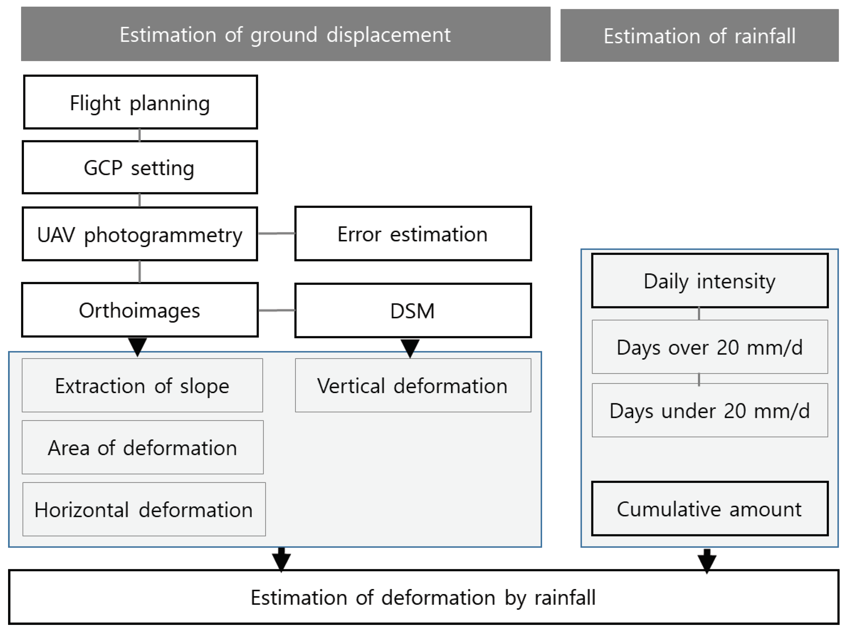
Figure 2.
Location of research area.
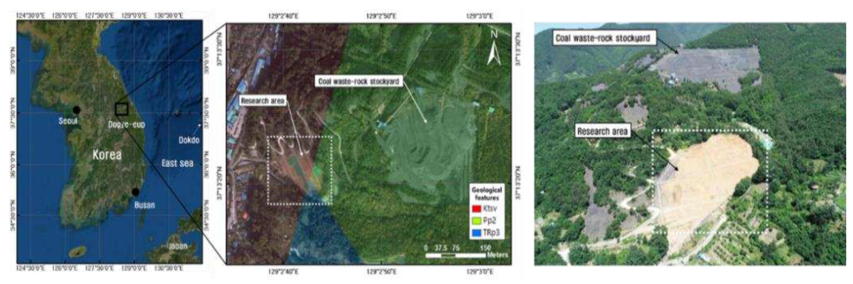
Figure 3.
Field survey measurements, (A) GCPs measuring equipment, (B) Remote-controlled UAV with camera set.
Figure 3.
Field survey measurements, (A) GCPs measuring equipment, (B) Remote-controlled UAV with camera set.
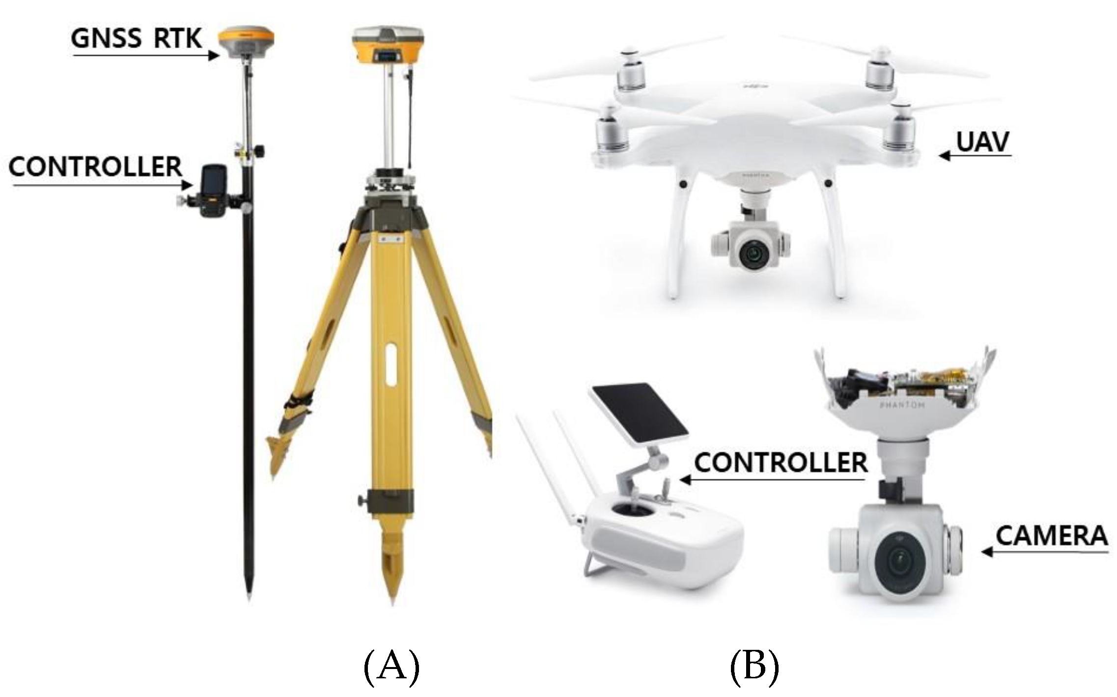
Figure 4.
UAV photogrammetry and flight path. (A) April 3, 2019. (B) October 13, 2019, (C) December 22, 2019. (D) April 10, 2020. (E) July 16, 2020. (F) August 14, 2020.
Figure 4.
UAV photogrammetry and flight path. (A) April 3, 2019. (B) October 13, 2019, (C) December 22, 2019. (D) April 10, 2020. (E) July 16, 2020. (F) August 14, 2020.
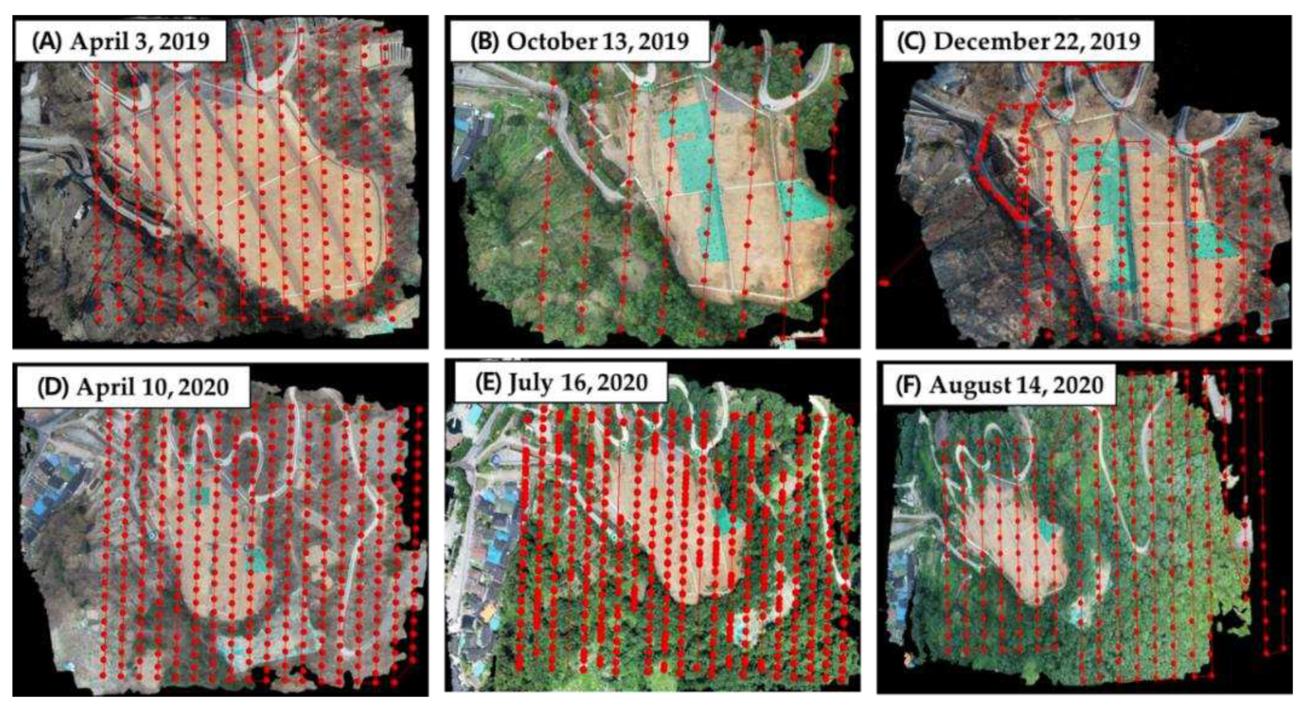
Figure 5.
Location of GCPs (A) April 3, 2019. (B) October 13, 2019, (C) December 22, 2019. (D) April 10, 2020. (E) July 16, 2020. (F) August 14, 2020.
Figure 5.
Location of GCPs (A) April 3, 2019. (B) October 13, 2019, (C) December 22, 2019. (D) April 10, 2020. (E) July 16, 2020. (F) August 14, 2020.
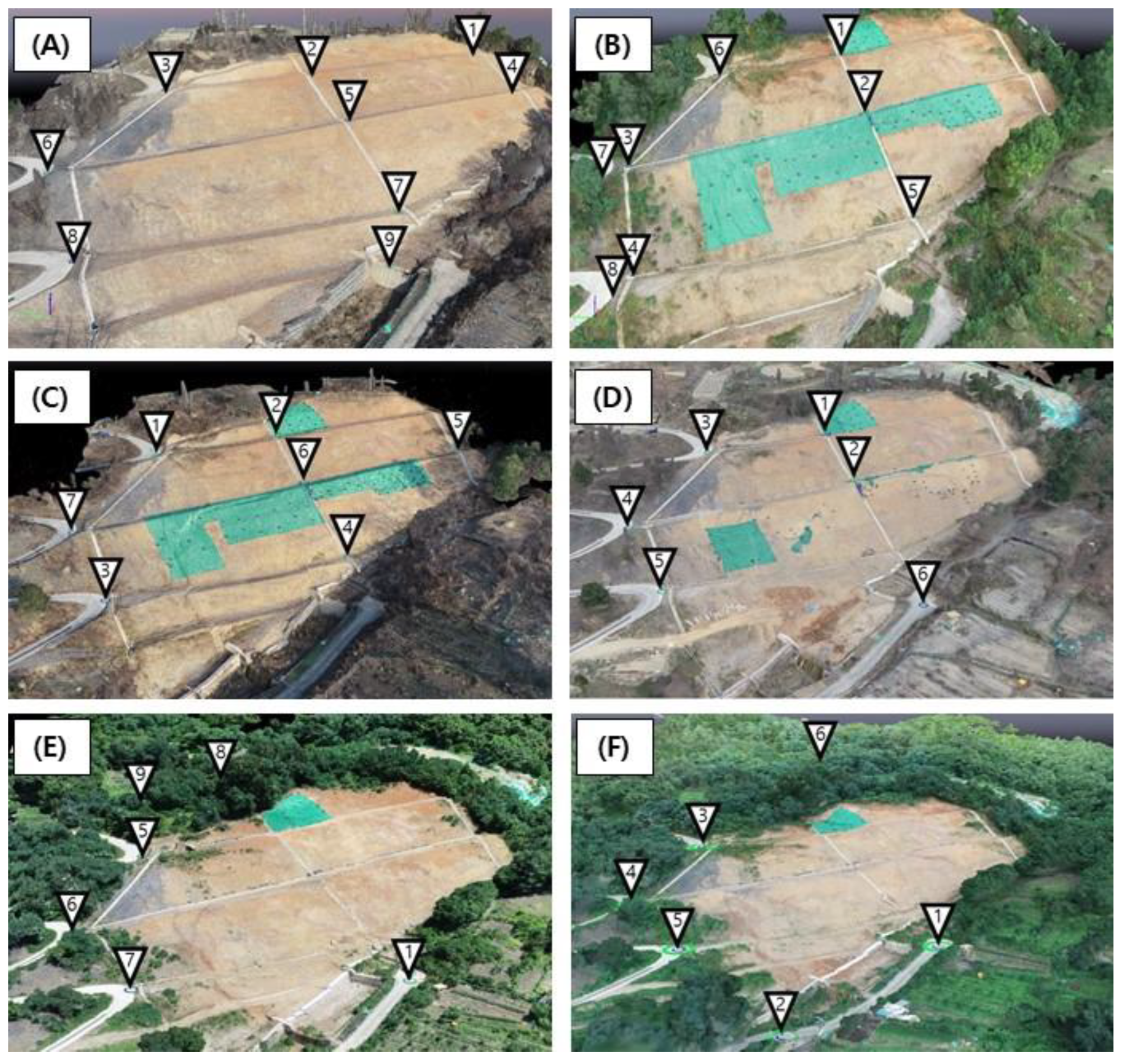
Figure 6.
Orthoimages at each period.
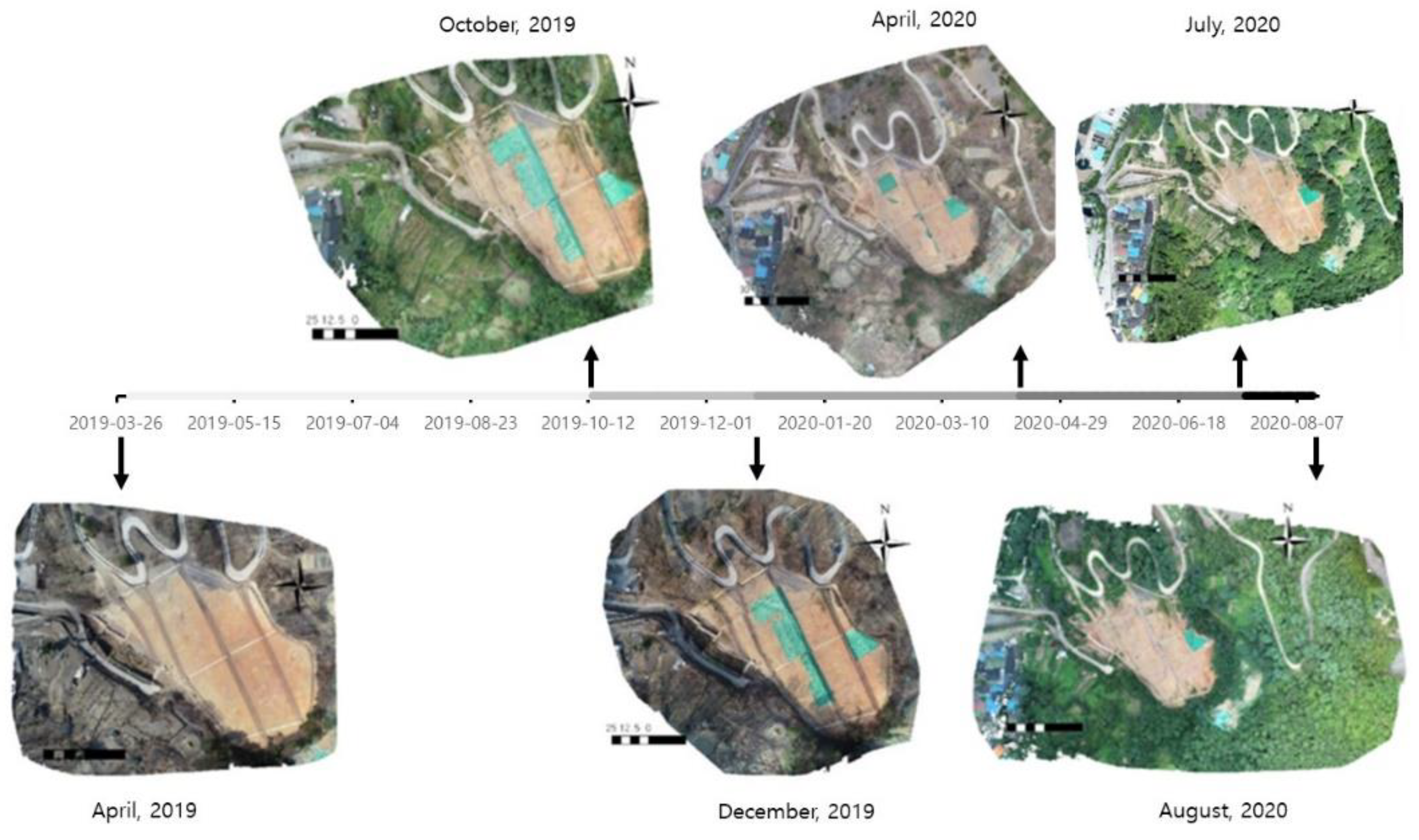
Figure 7.
Displacement area determined using DSM.
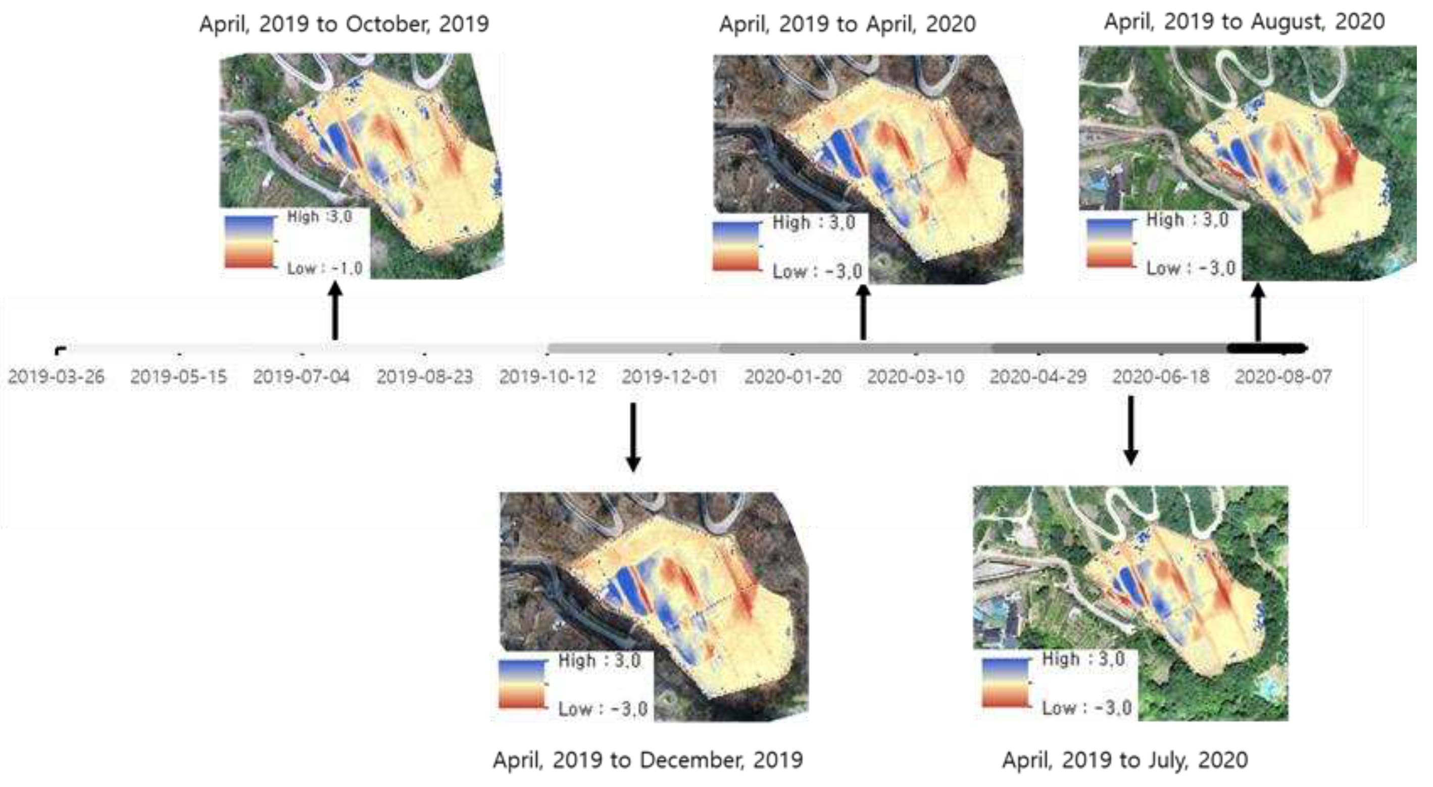
Figure 8.
Sketch of the photogrammetric area (A), baselines based on UAV derived orthoimage (B), and DEM map (C).
Figure 8.
Sketch of the photogrammetric area (A), baselines based on UAV derived orthoimage (B), and DEM map (C).
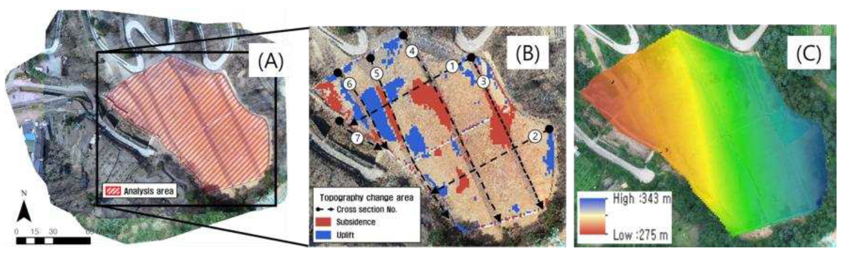
Figure 9.
The vertical deformation on baseline ①.
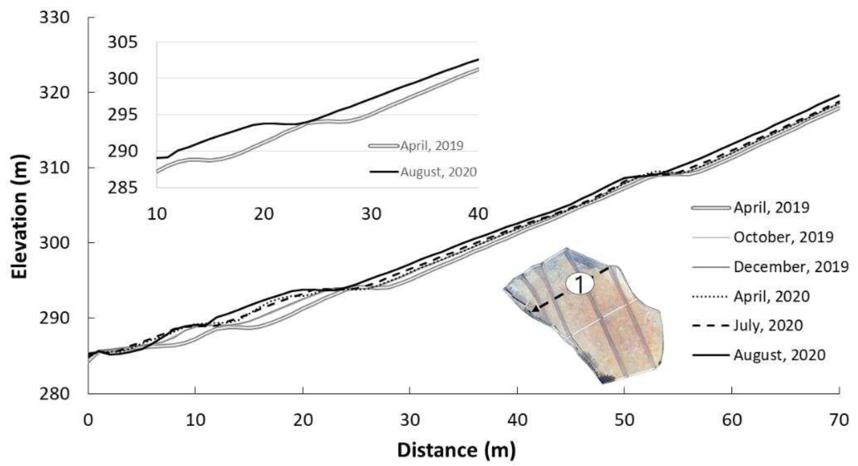
Figure 10.
Time series of elevation change on baseline ①.
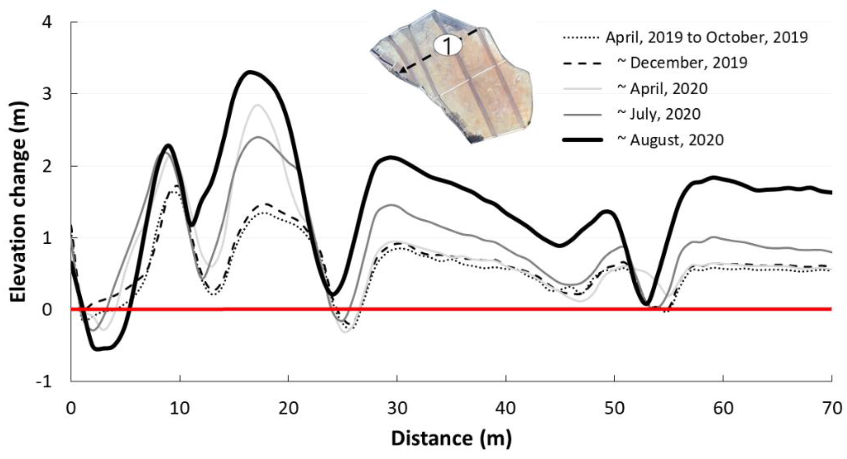
Figure 11.
The vertical deformation on baseline ② and detailed figure.
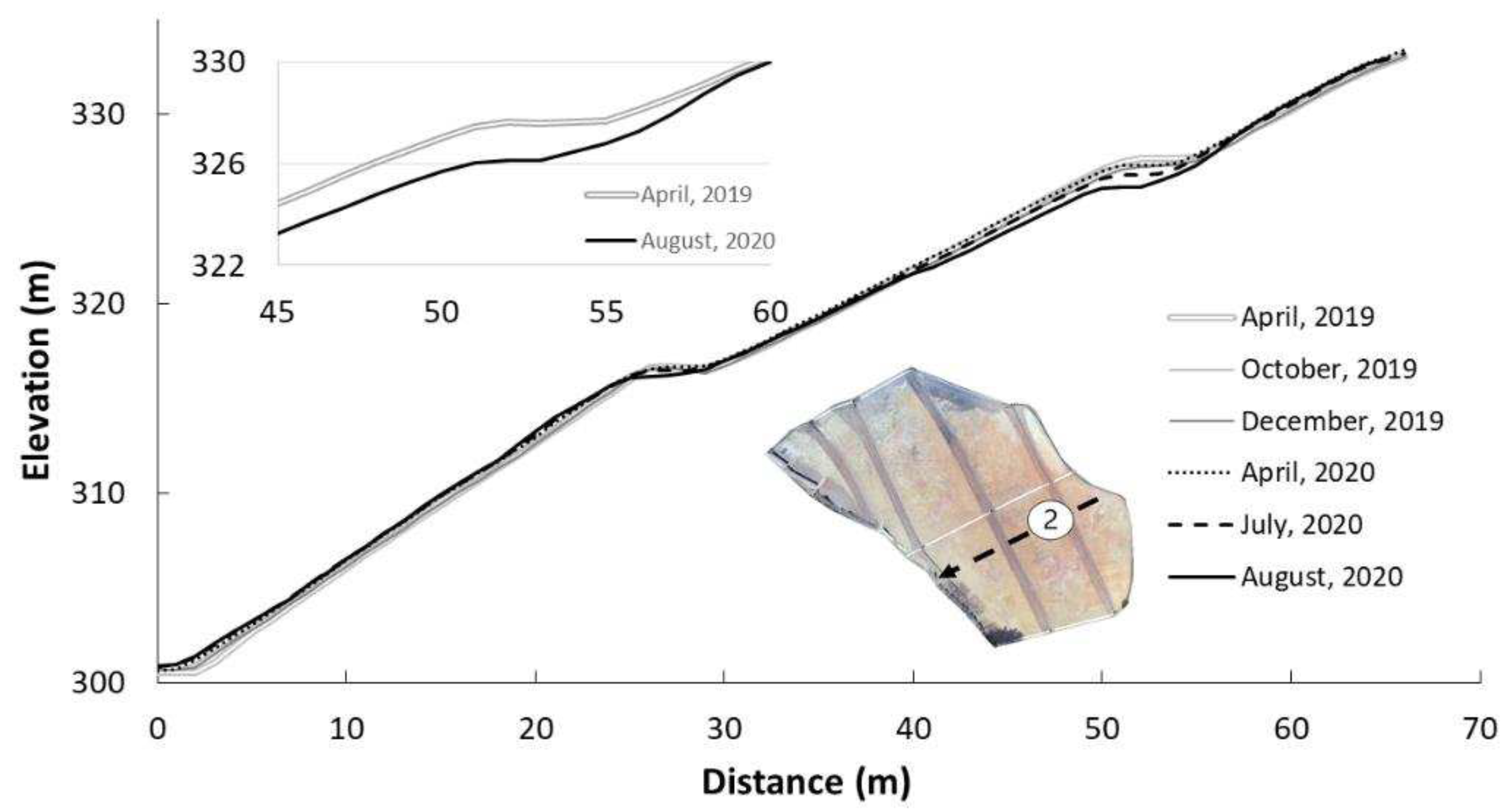
Figure 12.
Time series of elevation change on baseline ②.
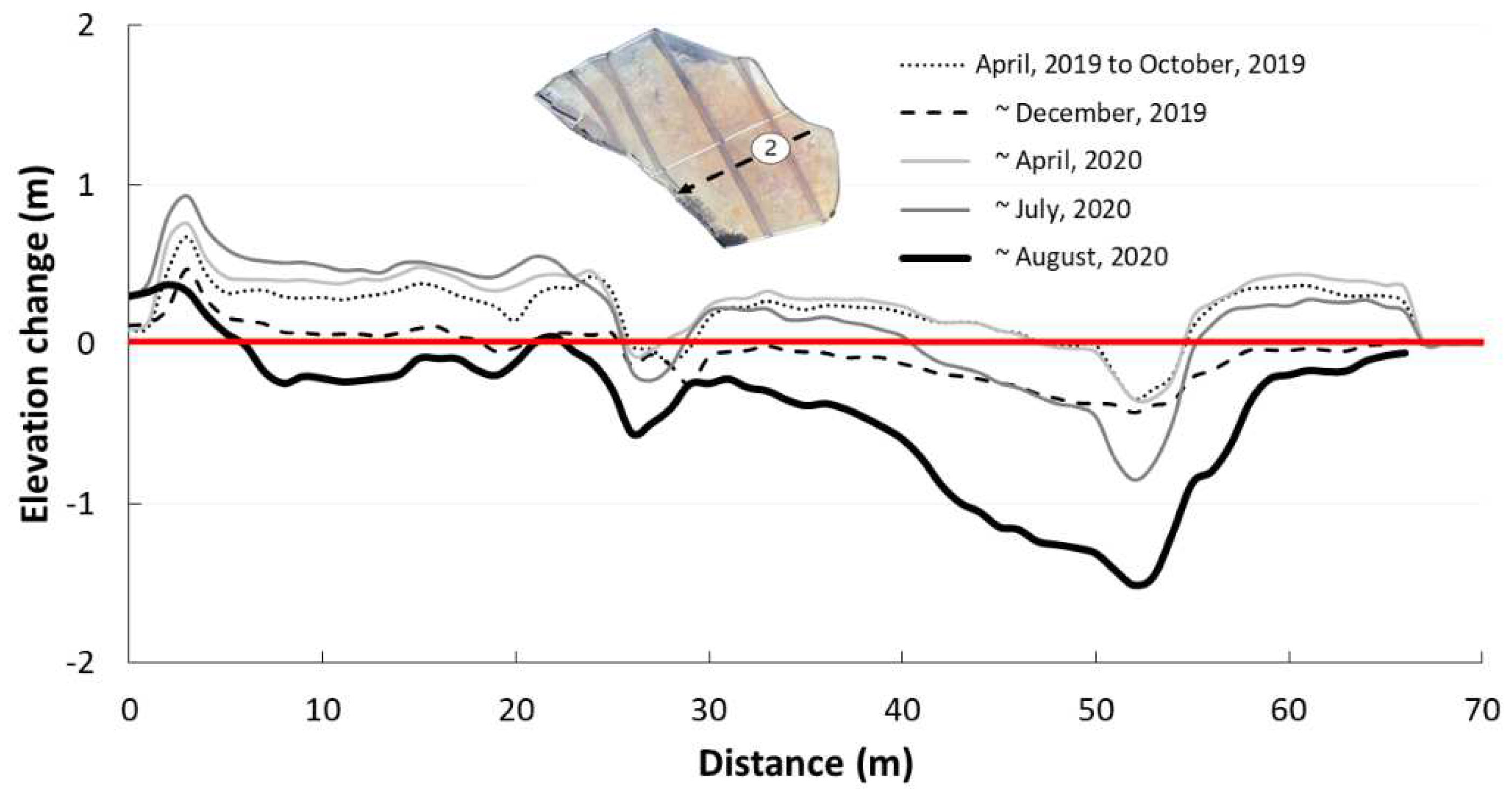
Figure 13.
Displacements determined using UAV photogrammetry. (A) Location of baselines. (B) Deformation drainage system. (C) Horizontal displacement between April and October 2019.
Figure 13.
Displacements determined using UAV photogrammetry. (A) Location of baselines. (B) Deformation drainage system. (C) Horizontal displacement between April and October 2019.

Figure 14.
Horizontal displacements on each baseline. (A) Baseline ③. (B) Baseline ④. (C) Baseline ⑤. (D) Baseline ⑥.
Figure 14.
Horizontal displacements on each baseline. (A) Baseline ③. (B) Baseline ④. (C) Baseline ⑤. (D) Baseline ⑥.
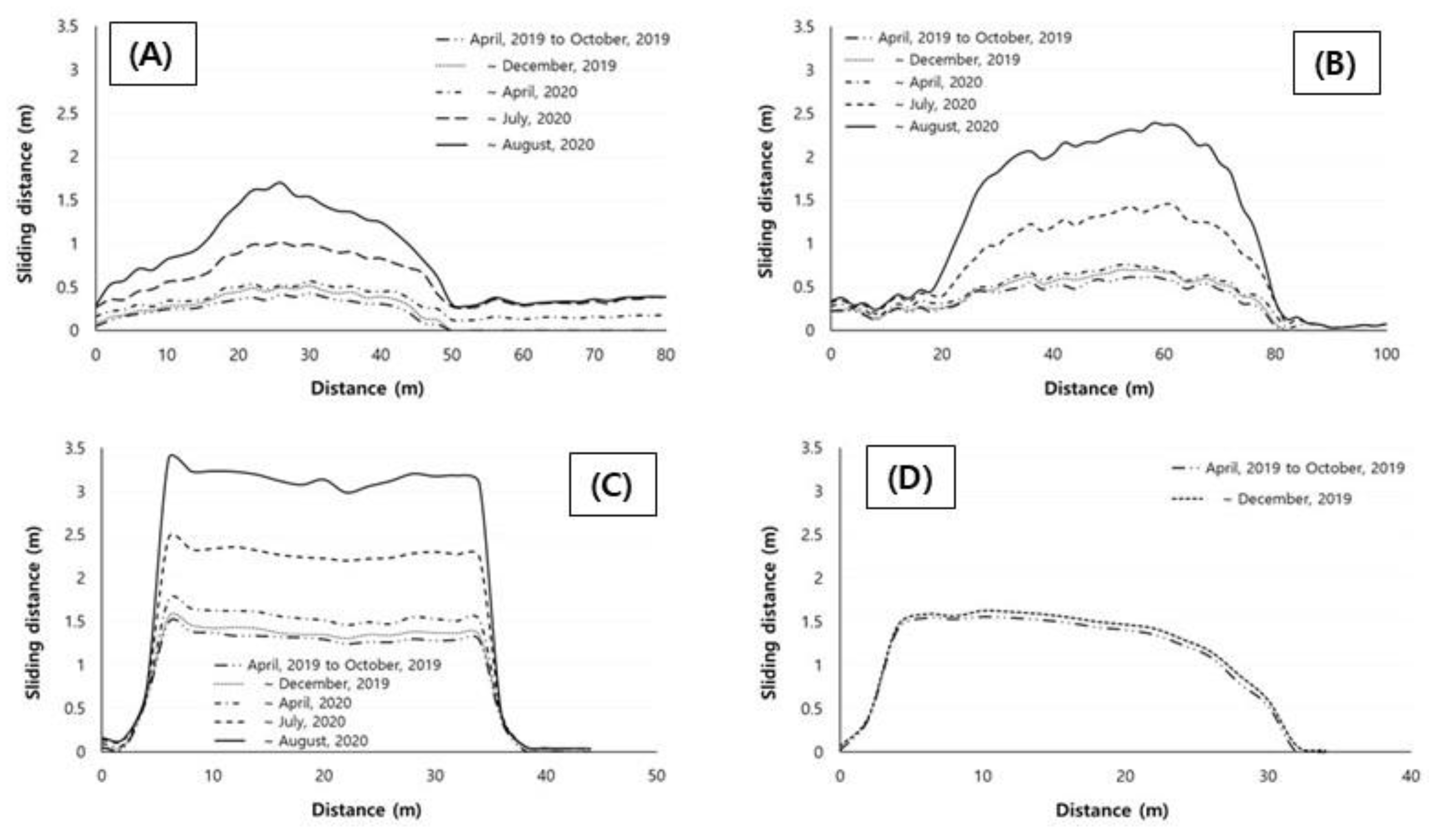
Figure 15.
Deformation of retaining wall due to ground movement. (A) Orthoimage on April 2019. (B) Orthoimage on October 2019. (C) Overlapped orthoimage.
Figure 15.
Deformation of retaining wall due to ground movement. (A) Orthoimage on April 2019. (B) Orthoimage on October 2019. (C) Overlapped orthoimage.
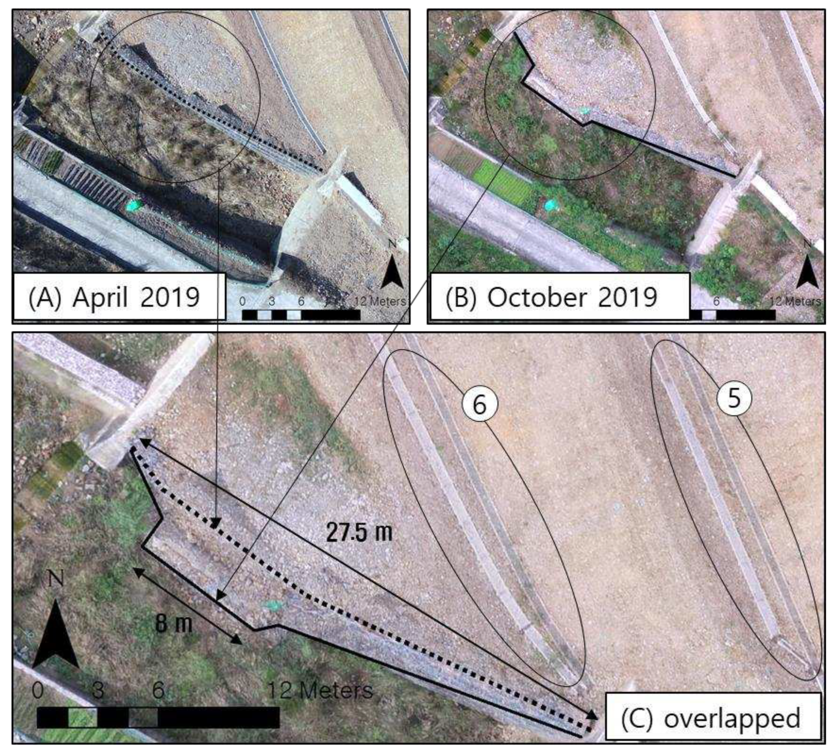
Figure 16.
Rainfall intensity between April 2019 and August 2020.
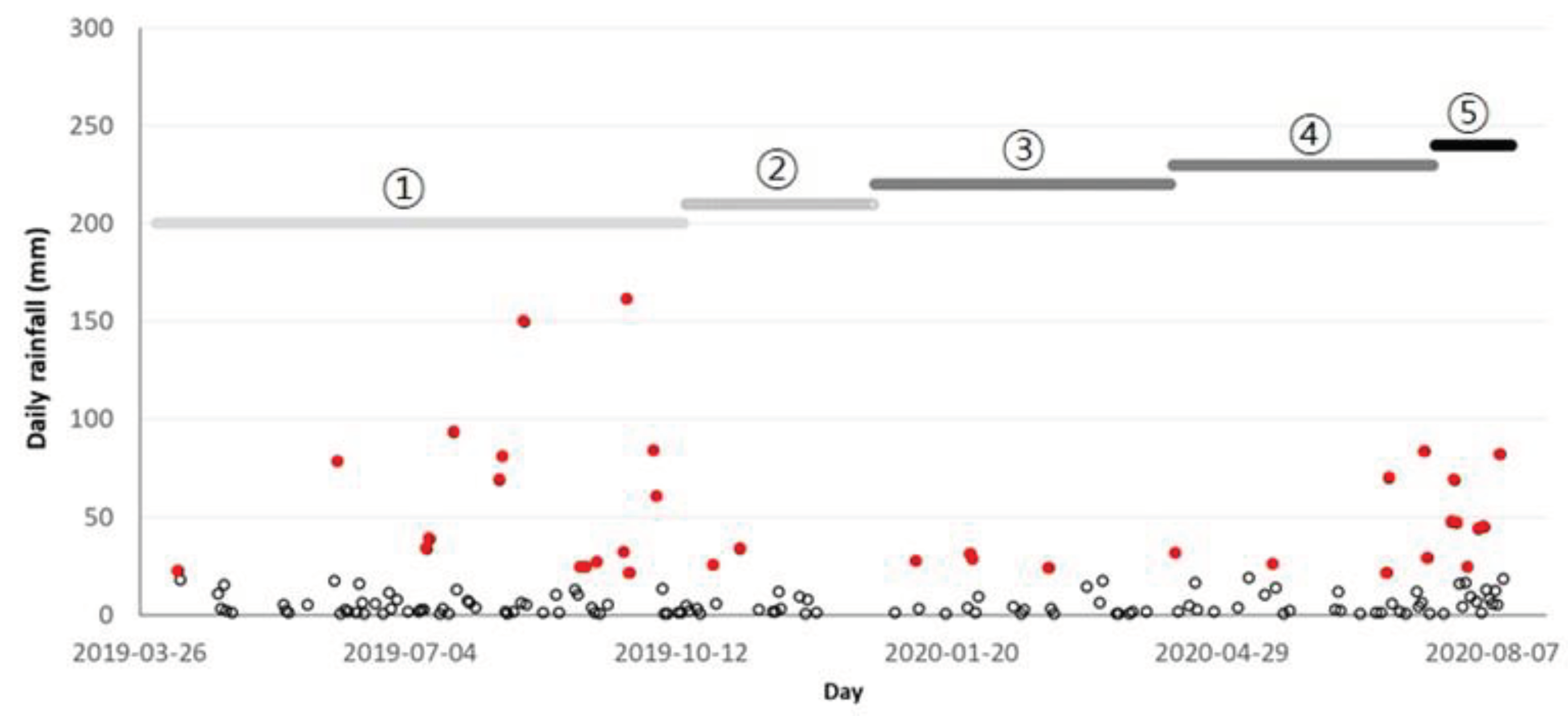
Figure 17.
Relationship between rainfall intensity and ground displacement.
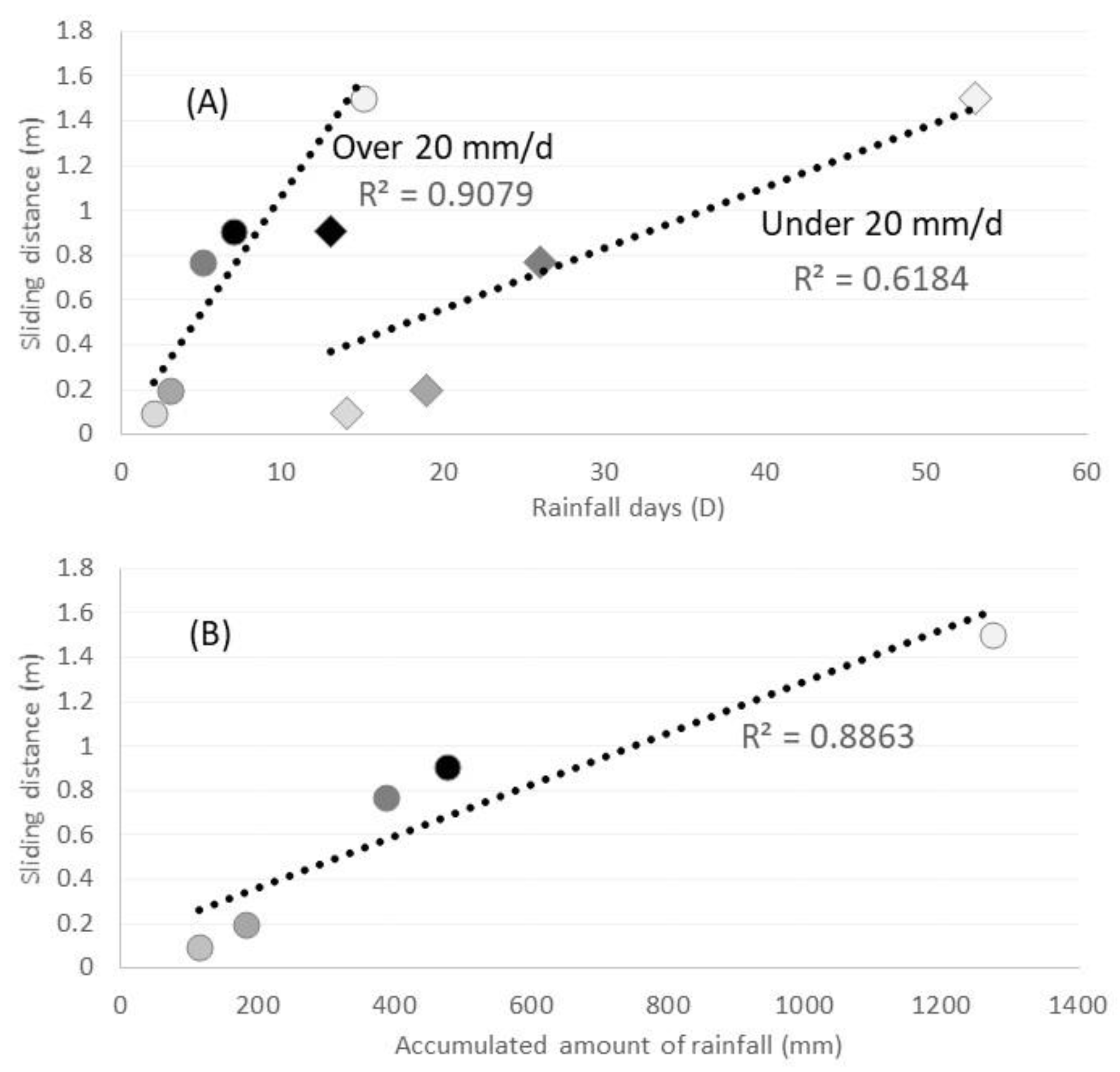
Table 1.
Summary of the UAV photogrammetric flight.
| April 3, 2019 | October 13, 2019 | December 22, 2019 | April 10, 2020 | July 16, 2020 | August 14, 2020 | |
| Temperature (℃) | 4.1 | 10.4 | 2.7 | 6 | 22.7 | 25.8 |
| Wind speed (m/sec) | 3.7 | 1.1 | 3.1 | 2.8 | 3.9 | 2 |
| Flight height (m) | 50 | 60 | 60 | 65 | 70 | 90 |
| Flight speed (m/sec) | 1.9 | 3.2 | 1.4 | 2.8 | 3.9 | 3.4 |
| Photogrammetry area (km2) | 0.042 | 0.029 | 0.032 | 0.075 | 0.072 | 0.080 |
| Overlap rate (%) | 90 | 80 | 87 | 87 | 90 | 90 |
| Number of images | 305 | 104 | 213 | 395 | 477 | 278 |
| Ground Sampling Distance (cm) | 2.12 | 1.96 | 1.64 | 1.76 | 2.13 | 2.09 |
Disclaimer/Publisher’s Note: The statements, opinions and data contained in all publications are solely those of the individual author(s) and contributor(s) and not of MDPI and/or the editor(s). MDPI and/or the editor(s) disclaim responsibility for any injury to people or property resulting from any ideas, methods, instructions or products referred to in the content. |
© 2023 by the authors. Licensee MDPI, Basel, Switzerland. This article is an open access article distributed under the terms and conditions of the Creative Commons Attribution (CC BY) license (http://creativecommons.org/licenses/by/4.0/).
Copyright: This open access article is published under a Creative Commons CC BY 4.0 license, which permit the free download, distribution, and reuse, provided that the author and preprint are cited in any reuse.


