
Submitted:
07 November 2024
Posted:
11 November 2024
You are already at the latest version
Abstract
One of the keys towards sustainable policies and advanced air quality monitoring is the detailed assessment of all factors that affect the surface concentrations of greenhouse gases and aerosols. While the development of new atmospheric tracers can pinpoint emission sources, the atmosphere itself plays a relevant role even at local scales: its dynamics can increase, or reduce, surface concentrations of pollutants harmful for human health and the environment. Peplosphere, or PBL (Planetary Boundary Layer), variability is known to affect such concentrations. In this study, an unprecedented characterization of PBL cycles and patterns is performed at the WMO/GAW regional coastal site of Lamezia Terme in Calabria, Southern Italy, in conjunction with the analysis of key greenhouse gases and aerosols. The analysis, accounting for five months of 2024 data, indicates that PBL variability and wind regimes do influence the concentrations of key GHGs and aerosols. In particular, eastern synoptic flows at the site are linked with high yields, and PBLH patterns can further influence the surface concentrations of carbon monoxide (CO), black carbon (BC), and particulate matter (PM). This research demonstrates that PBL monitoring needs to be considered when ensuring optimal air quality in urban and rural areas.
Keywords:
Lamezia Terme
; GAW
; sustainability
; Peplosphere
; Planetary Boundary Layer
; Atmospheric Boundary Layer
; Mediterranean basin
; greenhouse gas
; aerosol
; synoptic flow
1. Introduction
The Peplosphere, also referred to in literature as Planetary Boundary Layer (PBL) or Atmospheric Boundary Layer (ABL), is the lowest part of the atmosphere. The PBL is heavily influenced in its dynamics by constant contact with Earth’s surface [1,2,3,4,5,6]; it is also characterized by turbulences, vertical currents, distinct temperature profiles, and air flows which are not parallel to either the surface or isobars [7,8,9,10]. Only in the free atmosphere above the PBL air flows are mostly geostrophic [11,12].
The PBL has a well-defined diurnal-nocturnal cycle [13,14,15,16,17,18,19], which also results in peculiar dynamics directly affected by this cycle [20,21,22,23,24]. PBLH (Planetary Boundary Layer Height) is among the key parameters used in research to characterize peplospheric variability over time [25,26,27]. The PBLH is normally described as the height of the inversion level separation between the free troposphere above from the boundary layer [14]. In addition to the physical boundary of the PBL, it is worth mentioning that it possesses peculiar characteristics in terms of microbial ecology [28,29].
Research demonstrated correlations between PBLH and the concentration of several greenhouse gases and aerosols: therefore, PBL control over the surface concentration of these compounds is among the factors that can help predicting their variability and diffusion [30,31,32,33,34,35,36,37]. This also has a number of implications in terms of human health and environmental protection, as higher concentrations can lead to hazards [38,39,40]. For example, in the case of black carbon (BC) an inverse correlation with PBL height was demonstrated in areas affected by anthropogenic pollution [41]. In a world that is constantly dealing with climate change, air quality issues and the need for sustainable policies and regulations [42], additional knowledge on the PBL may be required.
In research, two main methods for PBLH measurement are used: the Gradient Method, and the Threshold Method. The former estimates PBLH by pinpointing the height of the minimum backscatter gradient [43,44,45,46,47], while the latter estimates PBLH as the threshold at which the backscatter signal is below a certain value [45,48].
In addition to the complexities of surface-PBL-free atmosphere interactions that normally occur on Earth, a significant role in PBL dynamics is played by the presence of sea/ocean masses, continents, and coastal boundaries below [8,49,50,51,52,53,54,55,56]. These extra complexities require ad hoc methodologies to assess PBL variability in these environments [57,58,59].
A better understanding of peplospheric influences over the concentration of GHGs and aerosols is necessary for provide regulators and policymakers with additional tools to better manage air quality issues in urban and rural areas. Various parameters affect air quality and local air pollution; this research paper will focus on three gases and two aerosol types.
Carbon dioxide (CO2) is the main driver of present-day anthropogenic climate change [60,61,62] and is therefore subject to monitoring on local to global scales [63,64]. Although CO2 does not pose the same health hazards as other atmospheric pollutants, it can impact the environment [65,66] and trigger long-term effects on human health [67,68,69]. Fossil fuel burning is the main source of anthropogenic CO2 in the atmosphere [70].
Carbon monoxide (CO) is an effective tracer of combustion and can be both natural and anthropogenic in origin. Wildfires are a prominent source of CO in the atmosphere [71] and the multi-year variability of this gas has shown a generally downward trend [72] that followed years of constant increases [73]. The decrease rate of CO has reduced in the past few years, indicating changes in the total global budget [74]. Although carbon monoxide is short-lived, it is known to play a role in the increase of methane [75] and surface ozone (O3) [76].
Methane (CH4) is heterogeneous in origin, with anthropogenic [77,78] and natural [79] sources contributing to its global budget. It is also a byproduct of fuel combustion [80,81]. Due to its high GWP (global warming potential) compared to CO2, CH4 emission reductions are one of the main challenges of present-day climate change mitigation [82].
Black carbon (BC) is a notable byproduct of combustion processes [71] and acts as both a driver of climate change [83,84,85] and a factor of health hazard [86]. Its effects are partially counterbalanced by a short persistence rate in the atmosphere, as BC has been observed to last for days [87,88].
Particulate matter (PM) is a common byproduct of vehicular emissions in urban areas [89,90] but can also be originated by several natural processes [91,92,93]. PM constitutes a significant health hazard due to its small size and the consequent capacity to affect lungs directly [94,95]; for this reason, it is subject to constant monitoring at various levels [96]. Several research studies have reported significant correlations between PBL and particulate patterns, thus showing that research on PBL variability also has implications for air quality and the sustainable development of urban and rural areas [97,98,99,100,101].
Previous research aimed at the WMO/GAW (World Meteorological Organization – Global Atmosphere Watch) observation site of Lamezia Terme (code: LMT) in the southern Italian region of Calabria was limited to data gathered during a summer 2009 campaign (specifically, from July 12th to August 6th) [102]. The campaign allowed the characterization of the main features of peplospheric variability at LMT, however, at the time there were no measurements of greenhouse gases and aerosols available. A further characterization of PBL influences over the concentration of pollutants was focused on the 2015 solar eclipse [103], but the study could not provide additional details on variability over time.
This study is therefore aimed at an unprecedented analysis of PBL variability at LMT, as well as its correlations with the patterns of key greenhouse gases and aerosols. This research is divided as follows: section 2 describes the LMT site, its instruments and datasets; section 3 will show the results of this campaign; sections 4 and 5 cover the discussion and results, respectively.
2. The Station, Methods, Instruments, and Datasets
2.1. The Observation Site and Its Characteristics
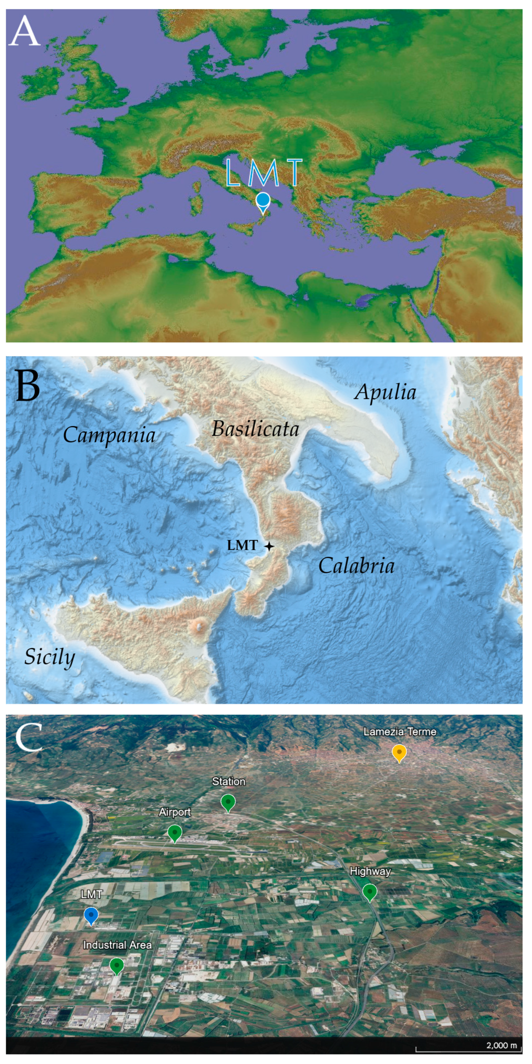
Fully operated by the National Research Council of Italy – Institute of Atmospheric Sciences and Climate (CNR-ISAC), the observation site (code: LMT; Lat: 38.88 N°; Lon: 16.23 E°; Elev: 6 m.a.s.l.) is located in the southern Italian region of Calabria, in the municipality of Lamezia Terme (Figure 1). The station is located 600 meters from the Tyrrhenian coast of the region (Figure 1), in an area known to be the narrowest point in the entire Italian peninsula, as the distance between the Tyrrhenian and Ionian coasts is ≈30 kilometers. This area, known as the Catanzaro isthmus, effectively separates the coastal chain (Catena Costiera) and Sila Massif in the north, from the Serre Massif in the south. The presence of two seas, with the Calabria region in between, results in increased meteorological instability, and oftentimes results in the occurrence of floods in the area [104,105,106].
Local wind circulation patterns in the western part of the isthmus were characterized in two 2010 studies by Federico and collaborators, which demonstrated the presence of a well-defined west-east local circulation [107,108]. In fact, the Lamezia Terme International Airport (IATA: SUF; ICAO: LICA), located 2 kilometers north of the LMT observatory, has a 10/28 (100/200 °N) runway orientation and local air traffic is subject to the same wind regime. Vertical wind profiles were characterized in a consequent study [109], which integrated previously gathered data on preliminary PBL characterization at the site [102]. A cross-study on multiple southern Italian stations also performed a PBL characterization via WRF modeling and related methodologies, however, the study was limited to one month of data from the 2009 summer season and did not evaluate GHGs or aerosols [110].
Measurements of greenhouse gases and other key parameters at the site started in 2015. The first study evaluating the results, Cristofanelli et al. (2017) [111], provided new insights on the characterization of LMT as what we would be later defined as a “multisource” site. The study also indicated that local wind circulation patterns, characterized in earlier studies [107,108], have a direct influence on LMT observations: western-seaside winds generally yield low concentrations, while northeastern-continental winds are linked with higher mole fractions of GHGs. With respect to aerosols, a more detailed description was performed in Donateo et al. (2018) [112].
Seven years (2016-2022) of methane data at LMT have been evaluated in D’Amico et al. (2024a) [113] and confirmed the influence of wind regimes on CH4 mole fractions with additional detail and also provided new insights on seasonal cycles: the highest mole fractions The study also found evidence of a HBP (Hyperbola Branch Pattern), with the highest mole fractions linked to low wind speeds and, vice versa, the lowest fractions linked to high speeds. The study D’Amico et al. (2024d) [114] on nine years (2015-2023) of surface ozone (O3) data however demonstrated that these patterns do not apply to all parameters, as ozone maxima are linked to spring/summer diurnal winds from the western sector. These opposite patterns observed at LMT underlined the complexity of parameters and how they combine with local wind circulation.
Figure 1.
A: Modified Copernicus Digital Elevation Model [115]. B: Modified EMODnet [116] highlighting LMT’s location in Southern Italy. C: Google Earth map, tilted by 70°, showing the observation site and key infrastructural/emission hotspots in the area. The “Highway” label indicates a point where the distance between LMT and the highway is ≈4.2 kilometers. The “Lamezia Terme” label points to the town center. The “Station” label points to the busiest train station in the municipality of Lamezia Terme, the central one (Lamezia Terme Centrale).
Research studies on LMT data also focused on weekly trends under the assumption that they can only be anthropic in nature, unlike natural trends such as the daily, seasonal, and yearly cycles. In D’Amico et al. (2024c) [117], the first COVID-19 lockdown period of 2020 was used to further assess local sources in a context of exceptionally limited anthropic activities. In fact, the restrictions introduced by the Italian government at the time [118] preceded similar measures issued by other European countries by days or even weeks, thus allowing changes in LMT data to be linked to local changes in emission sources. A cross study on aerosol data from multiple southern Italian stations, LMT included, was performed by Donateo et al. (2020) [119] and provided new insights on local vehicular traffic influences on aerosol diffusion. A more detailed local characterization of weekly patterns was performed in D’Amico et al. (2024b) [120] and demonstrated different behaviors of GHGs and aerosols, possibly linked to changes in anthropogenic activities throughout the week.
2.2. Instruments, Methodologies, and Datasets
To retrieve the aerosol backscatter profiles at the monitoring site, a Lufft CHM 15k Nimbus ceilometer (Fellbach, Germany) operating within ALICEnet (Italian Automated LIdar–CEilometer network) was used. The network is coordinated by CNR-ISAC in partnership with other Italian research institutions and environmental agencies. ALICEnet measurements are currently usefully employed to detect the altitude and temporal evolution of cloud layers and track the transport of polluted or mineral dust aerosol plumes at different sites along the Italian peninsula. This ceilometer is a ground-based, monostatic, active remote sensing instrument based on the LiDAR (Light Detection and Ranging) technique and principle [123].
The Nimbus ceilometer observes backscattered profiles with a vertical resolution of 15 meters over 24 continuous hours per day. Data are averaged every 15 seconds. The operating range is between the surface (~15 meters) to 15000 meters. Technical details of the instrument are shown in Table 1.
Specifically, the LiDAR technique is used by the Nimbus to emit short light pulses facing directly upward. Cloud layers, precipitations, and aerosols present in the column scatter back the pulses. By analyzing flight time, the intensity of backscattering, and counted pulses, the main features of the vertical column can be determined. The output is used to evaluate PBLH influences on tropospheric greenhouse gas and aerosol transport and dispersion [124]. In particular, the topmost aerosol layer detected by ceilometer pulses and consequent backscatter is used to represent the PBLH itself [125]. The expression used to receive the normalized backscattered signal power is given below (Eq. 1) and is provided by the manufacturer [126]:
where Pc(r) is normalized backscattered signal power, Praw is raw backscattered profile (photon counts), b is the baseline, Cs is calibration constant, O(r) is the overlap function, and Pcalc is average test pulse intensity. The output is calibrated in order to attenuate backscattered pulse results. In this research study, negative attenuated signals have been filtered out.
P c( r) = (Praw -b)/(Cs*O(r)*Pcalc)
During diurnal time ranges, dense (and/or multiple) cloud or aerosol layers may alter the backscattering signal and generate noise due to attenuation. In order to optimize the accuracy of results, backscattering profiles data are 5 minutes averaged to improve the signal-to-noise ratio.
In addition to ceilometer outputs, additional data have been gathered and processed to assess correlations between PBLH, greenhouse gases, pollutants, and key meteorological parameters. All data have been aggregated on an hourly and daily basis to allow direct comparison between different parameters.
Particulate matter (PM) data in micrograms per cubic meter (μg/m3 or μg PCM) have been gathered by a Palas Fidas 200 S (Karlsruhe, Germany). The instruments provides both Cn (particle numbers) and PM concentrations, however in this study only the latter have been used. A Sigma-2 sampling head draws in ambient air with a flow rate of approximately 0.3 m3/h. Aerosol gathered from ambient air passes through the sampling tube, equipped with a drying section meant to prevent measurement distortion attributable to moisture particle, and is ultimately drawn by the aerosol sensor. Via a Lorenz-Mie light analysis, particle size is determined by the instrument. Particles move through an optically differentiated volume that is illuminated by a polychromatic LED source. In response, each particle emits an impulse of scattered light that is detected by the instrument at angles of 85 to 95 degrees. Measurements are performed every ≈5 seconds and the results have been aggregated on hourly and daily bases, differentiated by particle size.
Data on downward solar radiation in watts per square meter (W/m2) have been gathered by a Kipp & Zonen radiometer, model CNR4. The radiometer used at LMT relies on two pyrgeometers and two pyranometers to measure upward (LW, 4.5–42 μm) and downward (SW, 0.31–2.8 μm) irradiance. Uncertainty in these measurements, traced to the BSRN (Baseline Surface Radiation Network) standard, is approximately 1% [127]. Additional details are available in Lo Feudo et al. (2015) [128] and Romano et al. (2017) [103].
Carbon monoxide (CO), carbon dioxide (CO2), and methane (CH4) mole fractions in ppm (parts per million) have been gathered by a Picarro G2401 (Santa Clara, California, USA) CRDS (Cavity Ring-Down Spectrometry) analyzer [129]. Via the principle of CRDS, these carbon compounds in the atmosphere are measured with high degrees of precision. At LMT, the G2401 gathers continuous data and is subject to WMO-compliant calibration cycles. Additional details on G2401 data gathering, calibration procedures and quality assurance are available in Cristofanelli et al. (2017) [111], D’Amico et al. (2024a) [113], D’Amico et al. (2024b) [120], and D’Amico et al. (2024c) [117].
Key meteorological surface data have been gathered by a Vaisala WXT520 (Vantaa, Finland). The instrument relies on ultrasounds to monitor wind direction and speeds, and a transducer to gather temperature data. Additional details on WXT520 measurements at Lamezia Terme are available in D’Amico et al. (2024a) [113]
Equivalent black carbon (eBC) micrograms per cubic meter (μg/m3 or μg PCM) have been measured by a Thermo Scientific 5012 (Franklin, Massachusetts, USA). The instrument operates as a MAAP (Multi-Angle Absorption Photometer), measuring the short-wave absorption parameters of aerosol [130,131,132]. Specifically, the aerosol absorption coefficient (sa), and equivalent black carbon are measured at 637 nm. Additional details are available in Calidonna et al. (2020) [121], D’Amico et al. (2024b) [120], and D’Amico et al. (2024c) [117].
Particle scattering and hemispheric backscattering coefficients at 450, 525, and 635 nanometers (nm) were measured by a LED-based integrating nephelometer (model Aurora 3000, ECOTECH, Knoxfield, Australia) at a temporal resolution of one minute. Air sampling was obtained from the top of a stainless steel tube having a 15 mm internal diameter and a length of ≈1.5m. The inlet was fitted with a funnel covered by a screen to prevent rain drops and arthropods from reaching the sample line. No aerosol size cut-off was applied to the sampled air, and a relative humidity threshold of 60% was set by a processor controlled automatic heater inside the nephelometer to prevent the hygroscopic effects that enhance particle scattering.
Each instrument and its respective dataset has been processed and quality-checked. Data coverage rates (%) compared to the actual number of days (153) and hours (3672) elapsed between May 1st 2024 and September 30th 2024 are shown in Table 2.
Using meteorological data, days have been divided into four categories (plus a fifth “NA” category not matching any of the requirements, which is hereby excluded). The “Breeze” regime has been defined as alternating wind directions (WD) between 270 and 70 degrees N, and wind speeds (WS) in the 2-6 m/s interval. The “Eastern Synoptic” regime is defined with a constant WD of 70°, and WS ≥6 m/s. The “Western Synoptic” has the same WS threshold as its eastern counterpart, but the WD is 270°. The “Not Complete” breeze regime is applied to days with a growing breeze regime which was later overcome by a regime leaning to western synoptic characteristics. In this case, the WS threshold is within 4-8 m/s. All reported WD have an applicability range of ±15°. Table 3 shows how days whose wind regime falls in one of the above-mentioned categories are distributed over the observation period.
3. Results
3.1. Daily Variability During the Observation Period
The campaign evaluated in this study accounts for five months of data gathering at LMT, from May 1st to September 30th 2024. As described in section 2.1, the Lamezia Terme regional WMO/GAW station is affected by cyclic wind patterns. Figure 2 shows a wind rose based on hourly-aggregated wind speeds and directions.
Data on CO, CO2, CH4, eBC, and PM have been gathered on a daily basis to highlight possible trends during the campaign. As reported in Table 2, the coverage rates of these findings vary depending on instrument maintenance and quality assurance. Figure 3 shows hourly aggregated data of all five parameters, with PM data being further divided into multiple sub-categories.
The same analysis has been applied to meteorological and environmental data. Figure 4 shows the daily averages of primary data gathered at LMT during the campaign.
In addition to daily averages, hourly aggregations have also been computed to show variations between May and September 2024 with enhanced details. Figure 5 and Figure 6 show these aggregates for GHG/aerosol and environmental parameters, respectively. Y axes scales have been adjusted to account for observed peaks.
3.2. Daily Cycles
Research studies on LMT data highlighted the existence of daily cycles [111,113,114], which are affected by local wind circulation patterns. Up until the campaign presented in this research, these cycles were not shown considering the influence of wind regimes. Figure 7 therefore shows an enhanced evaluation of the LMT daily cycle of greenhouse gases and aerosol accounting for the four categories described in section 2.2. Figure 8 shows the daily cycle of key environmental and meteorological parameters.
3.3. Percentile Roses
In D’Amico et al. (2024d) [114], percentile roses have been used to correlate surface ozone concentrations at LMT with specific wind directions. The same method has been used in this research for CO, CO2, CH4, eBC, and PM, with the results being reported in Figure 9. PM2.5 and PM10 have been plotted separately.
3.4. PBL Variability and Cycles
Following the evaluation seen in the previous sections with respect to GHGs, aerosols, meteorological, and environmental parameters, the PBLH at Lamezia Terme has been also characterized using daily and hourly averages. The results are shown in Figure 10.
Vertical profiles of select days deemed representative of all wind regimes have also been plotted using Nimbus data. The results are shown in Figure 11.
3.5. Correlations Between PBLH, Gases and Aerosols
Scatter and quantile–quantile plot (qplots) of observed parameters (x axis) have been correlated with PBLH (y axis) in Figure 12, Figure 13, Figure 14, Figure 15, Figure 16 and Figure 17. Colored squares indicate the amount of data in each 0.1x0.1 bin. Green lines represent the quantile–quantile plots, and red lines the least-square best fits. For each parameter, the top plots show breeze and not complete breeze regimes, while the bottom ones show western and eastern synoptic flow data, respectively.
4. Discussion
A campaign focused on Planetary Boundary Layer (PBL) characterization has been performed at the Lamezia Terme regional WMO/GAW observation site in Calabria, Southern Italy. The campaign relied on a new ceilometer (Table 1), a longer observation span compared to previous comparable research, and the integration of additional data (specifically, greenhouse gases and aerosols, see Table 2) meant to test correlations that were not applicable during the summer 2009 campaign described in Lo Feudo et al. (2020) [102].
The preliminary evaluation of environmental parameters allowed to define the fundamentals upon which the findings of this campaign would be based on. Local wind circulation patterns are oriented on a W/NE axis [107,108], as shown in Figure 2. Greenhouse gas and aerosol data coverage, in addition to meteorological parameters, show both daily (Figure 3 and Figure 4) and hourly (Figure 5 and Figure 6) variability during the observation period.
Following the analyses seen in other research papers focused on LMT data [111,113,114,117], daily cycles of greenhouse gases, aerosols, and meteorological parameters have been assessed. LMT has been proven in multiple studies to have a peculiar daily cycle and this research effectively integrates a new variable, peplosphere height variability, into these cycles.
In the case of GHGs and aerosols, the analysis has considered four distinct wind regimes, each defined by specific direction (WD) and speed (WS) thresholds: breeze, not complete (NC) breeze, eastern synoptic, and western synoptic (Table 3). In the case of CO2 (Figure 7B) and CH4 (Figure 7C), although the breeze and NC breeze yield higher values during night-time hours, diurnal concentrations are lower and do not show differences in terms of wind regime. However, CO (Figure 7A), eBC (Figure 7D) and PM (Figure 7E, 7F, 7G) show a greater variability in morning and evening hours that is compatible with inversions in wind patterns from the northeastern-continental to the western-seaside corridors, and vice versa. PM (Figure 7F, 7G) is particularly susceptible to night-time fluctuations. The susceptibility of pollutant concentrations to inversions in wind patterns was first reported in Cristofanelli et al. (2017) [111] and further supported in D’Amico et al. (2024c) [117], which analyzed the first 2020 COVID-19 lockdown in Italy to highlight the nature of pollutant peaks linked to wind circulation in lockdown versus ante/post lockdown periods.
Key meteorological and environmental parameters show well-defined daily cycles (Figure 8). In particular, SCA values (Figure 8D) show a peak linked to increased pollutant inversions that occur during inversions.
The percentile roses in Figure 9 differentiate between gases and aerosols in terms of spatial distribution. Two types of behavior are reported: minor spatial variations, as seen in the case of CO2 (Figure 9B) and CH4 (Figure 9C); intermediate variations, as in the case of CO (Figure 9A), eBC (Figure 9D), and PM2.5 (Figure 9F); substantial variations, seen specifically in PM10 (Figure 9G). These differences reflect not only the susceptibility of each parameter to wind regimes, but also indicate distinct emission sources. CO and eBC, which are both effective tracers of combustion processes, were linked to local wildfires in a previous research study by Malacaria et al. (2024) [122]. CH4 is characterized by both natural and anthropogenic sources, and local peaks are linked to northeastern-continental winds [113]. In Cristofanelli et al. (2017) [111], methane peaks at LMT were specifically attributed to sources located nearby.
Particulate matter and reported differences based on particle size are indicators of distinct emission sources. In fact, as described in section 1, PM is heterogeneous in nature. Anthropogenic PM2.5 emissions are generally linked, for example, to fossil fuel burning and domestic heating, while PM10 is linked to natural sources such as sea spray, biomass burning attributable to agriculture, Saharan dust events [121], and wildfires [122]. Among the anthropogenic sources of PM10, incomplete fossil fuel burning processes are common. The findings of this research study allow to narrow down the nature of observed PM depending on the four wind regimes that affect LMT observations: the breeze is linked to diurnal sea spray from the west and nocturnal smog from the northeast; the not complete (NC) breeze results into a southern corridor and PM peaks that are hereby interpreted as biomass burning linked to agricultural activities; the western synoptic combines sea spray outputs, combined with continental-anthropogenic PM; the eastern synoptic is linked to all PM categories.
In Figure 10, PBLH data have been plotted to show the overall variability during the observation period, as well as the daily cycle (Figure 10C). This cycle in particular shows daily PBLH variations dependent on the four distinct categories of wind regimes, which in turn have an impact on gas and aerosol concentrations observed at LMT. Examples of the four categories are shown in Figure 11.
Qplots testing the correlation of PBLH, gases and aerosols have been plotted in Figure 12 through 17 under all four wind regimes. An apparent inverse relationship or anticorrelation between PBLH and CO2 and CH4 concentrations can be seen in Figure 13 and Figure 14. This suggests that as the PBLH increases, CO2 and CH4 concentrations tend to decrease, indicating that lower peplosphere heights correspond to limited vertical mixing and the accumulation of these gases near the surface.
When synoptic conditions are favorable to sea breeze development, colder air masses from the sea with low marine aerosol content are advected over land in the early morning and interact with the nighttime boundary layer. After the onset of the sea breeze, an internal boundary layer develops from the coastal discontinuity and the height of the maximum backscatter threshold from the Nimbus decreases, likely due to the advection of the marine aerosols above the PBL, thus creating a discontinuity in aerosol concentration and size distribution. Later in the morning, when the breeze is well developed, the convection takes over and mixes marine and continental aerosols, creating a homogeneous content of aerosols filling the convective layer.
During stationary synoptic flow with wind speed typically >5 m/s, marine aerosols are mixed with their continental counterparts and the height of the boundary layer detected by LMT’s ceilometer remains constant. During sea breeze days, at the onset of the breeze, the findings of this research and past studies indicate that the sea breeze advection of marine aerosols causes a nonhomogeneous columnar distribution, inducing a low LiDAR signal-to-noise ratio above the internal boundary layer [102].
Figure 12, Figure 13, Figure 14, Figure 15, Figure 16 and Figure 17 show that the advection of cleaner air with marine aerosols from the sea with respect to the land aerosols, flowing above the internal boundary layer, after the breeze onset, causes a vertical discontinuity of aerosol concentration and thus a reduction of the LiDAR vertical range. In case of breeze, the resulting values of PBL vary as expected following the daily cycle over land, i.e., low during the stable night and high during the unstable days: during synoptic flow, the PBL is constantly higher compared to unstable conditions. It is therefore reported that during the night, synoptic PBLH is larger than during the day. A reason can be that during summer the breeze always develops, adding and modulating the synoptic flow (Figure 11). A well-developed breeze, adding speed, would produce a large quantity of marine aerosols advected on land flowing over the land; aerosol layer would contribute to the detection of a lower PBLH.
Therefore, the findings of this research provide evidence of direct peplospheric influences over the surface concentrations of greenhouse gases and aerosols.
5. Conclusions
This research work relied on an enhanced characterization of peplospheric variability at the Lamezia Terme (code: LMT) regional coastal WMO/GAW observation site in Calabria, Southern Italy. The study is based on five continuous months (May-September 2024) of PBL data obtained by a Nimbus ceilometer, plus greenhouse gas, aerosol, meteorological, and environmental data gathered by other instruments. The integration of multiple datasets has ensured a more detailed understanding of PBL variability at the site, as the previous campaign on PBL data was focused entirely on one month of observations performed during the 2009 summer season, and no correlations with the surface concentrations of key pollutants were possible at the time.
This study has introduced four distinct categories of wind regimes (breeze, not complete breeze, eastern synoptic, western synoptic) and tested the correlation of PBLH variability with the concentrations of carbon monoxide (CO), carbon dioxide (CO2), methane (CH4), equivalent black carbon (eBC), and particulate matter (PM) under each regime.
Overall, these findings demonstrate the need to effectively integrate PBLH data and wind regimes in urban air quality assessments due to the influence of PBLH patterns on the surface concentration of key pollutants. Such a study demonstrates the importance of correlating circulation, complex orography and boundary conditions at the interface between land and sea when dealing with the assessment of natural and anthropogenic pollutants. The availability of physical/chemical and aerosol data allows to test the correlation between PBLH variability and a number of factors.
The LMT observation site is therefore a challenging natural laboratory for capturing different circulation patterns in which natural and anthropic-induced pollutant concentrations show different behaviors. Future research integrating the findings shown in this study with additional parameters will further demonstrate the importance of considering all these factors in sustainable policies/regulations and air quality monitoring.
Author Contributions
Conceptualization, F.D. and T.L.F.; methodology, F.D. and T.L.F.; software, F.D., D.G., S.S., G.D.B. and T.L.F.; validation, C.R.C., I.A., D.G., S.S., G.D.B. and T.L.F.; formal analysis, F.D., D.G., G.D.B and T.L.F.; investigation, F.D., D.G., G.D.B and T.L.F.; data curation, F.D., I.A., D.G., L.M., S.S., G.D.B. and T.L.F.; writing—original draft preparation, F.D., C.R.C., T.L.F.; writing—review and editing, F.D., CR.C., I.A., D.G., L.M., S.S., G.D.B. and T.L.F.; visualization, F.D., C.R.C., D.G., L.M., S.S., G.D.B. and T.L.F.; supervision, C.R.C. and T.L.F.; funding acquisition, C.R.C. All authors have read and agreed to the published version of the manuscript.
Funding
This research was funded by AIR0000032 – ITINERIS, the Italian Integrated Environmental Research Infrastructures System (D.D. n. 130/2022 - CUP B53C22002150006) under the EU - Next Generation EU PNRR - Mission 4 “Education and Research” - Component 2: “From research to business” - Investment 3.1: “Fund for the realization of an integrated system of research and innovation infrastructures”.
Data Availability Statement
The datasets presented in this article are not readily available because they are part of other ongoing studies. ALICEnet data are available through the dedicated online platform.
Acknowledgments
To be filled in later (anonymous reviewers, editors).
Conflicts of Interest
The authors declare no conflicts of interest.
References
- Buajitti, K.; Blackadar, A.K. Theoretical studies of diurnal wind-structure variations in the planetary boundary layer. Boundary-Layer Meteorol. 1957, 83(358), 486-500. [CrossRef]
- Barry, P.J.; Munn, R.E. Use of radioactive tracers in studying mass transfer in the atmospheric boundary layer. Phys. Fluids 1967, 10(9), S263–S266. [Google Scholar] [CrossRef]
- Estoque, M.A.; Bhumralkar, C.M. A method for solving the planetary boundary-layer equations. Boundary-Layer Meteorol. 1970, 1, 169–194. [CrossRef]
- Godev, N. On the cyclogenetic nature of the Earth's orographic form. Arch. Met. Geoph. Biokl. A. 1970, 19, 299–310. [Google Scholar] [CrossRef]
- Clarke, R.H. Observational studies in the atmospheric boundary layer. Q. J. R. Meteorol. Soc. 1970, 96(407), 91–114. [Google Scholar] [CrossRef]
- Telford, J.W. The surface roughness and planetary boundary layer. PAGEOPH 1980, 119(2), 278–293. [Google Scholar] [CrossRef]
- Stewart, R.W.; Wilson, J.R.; Burling, R.W. Some statistical properties of small scale turbulence in an atmospheric boundary layer. J. Fluid Mech. 1970, 41, 141–152. [Google Scholar] [CrossRef]
- Van Atta, C.W.; Chen, W.Y. Structure functions of turbulence in the atmospheric boundary layer over the ocean. J. Fluid Mech. 1970, 44, 145–159. [Google Scholar] [CrossRef]
- Garratt, J.R.; Francey, R.J. Bulk characteristics of heat transfer in the unstable, baroclinic atmospheric boundary layer. Boundary-Layer Meteorol. 1978, 15(4), 399-421. [CrossRef]
- Schönwald, B. Determination of vertical temperature profiles for the atmospheric boundary layer by ground-based microwave radiometry. Boundary-Layer Meteorol. 1978, 15(4), 453-464. [CrossRef]
- Arya, S.P.S. Comparative effects of stability, baroclinity and the scale-height ratio on drag laws for the atmospheric boundary layer. J. Atmos. Sci. 1978, 35, 40–46. [Google Scholar] [CrossRef]
- Zhao, M. A numerical experiment of the PBL with geostrophic momentum approximation. Adv. Atmos. Sci. 1988, 5, 47–56. [Google Scholar] [CrossRef]
- Angell, J.K. Correlations in the vertical component of the wind at heights of 600, 1,600 and 2,600 ft at Cardington. Q. J. R. Meteorol. Soc. 1964, 90(385), 307–312. [Google Scholar] [CrossRef]
- Stull, R.B. An Introduction to Boundary Layer Meteorology; Kluwer Acad.: Dordrecht, The Netherlands, 1988; p. 666. [Google Scholar] [CrossRef]
- Stensrud, D.J. Parameterization Schemes: Keys to Understanding Numerical Weather Prediction Models; Cambridge University Press, UK, 2007; p. 459. [CrossRef]
- Liu, S.; Liang, X.Z. Observed diurnal cycle climatology of planetary boundary layer height. J. Clim. 2010, 23(21), 5790–5809. [Google Scholar] [CrossRef]
- Wang, W.; Gong, W.; Mao, F.; Pan, Z. An Improved Iterative Fitting Method to Estimate Nocturnal Residual Layer Height. Atmosphere 2016, 7(8), 106. [Google Scholar] [CrossRef]
- Bakas, N.A.; Fotiadi, A.; Kariofillidi, S. Climatology of the Boundary Layer Height and of the Wind Field over Greece. Atmosphere 2020, 11(9), 910. [Google Scholar] [CrossRef]
- Gu, J.; Zhang, Y.H.; Yang, N.; Wang, R. Diurnal variability of the planetary boundary layer height estimated from radiosonde data. Earth Planet. Phys. 2020, 4(5), 479–492. [Google Scholar] [CrossRef]
- Rao, K.S.; Snodgrass, H.F. Some parameterizations of the nocturnal boundary layer. Boundary-Layer Meteorol. 1979, 17, 15-28. [CrossRef]
- Mahrt, L.; Heald, R.C.; Lenschow, D.H.; Stankov, B.B.; Troen, I.B. An observational study of the structure of the nocturnal boundary layer. Boundary-Layer Meteorol. 1979, 17(2), 247-264. [CrossRef]
- Hsu, S.A. Mesoscale nocturnal jetlike winds within the planetary boundary layer over a flat, open coast. Boundary-Layer Meteorol. 1979, 17(4), 485-494. [CrossRef]
- Sawyer, V.; Li, Z. Detection, variation and intercomparison of the planetary boundary layer depth from radiosonde, lidar and infrared spectrometer. Atmos. Environ. 2013, 79, 518–528. [Google Scholar] [CrossRef]
- Coen, M.C.; Praz, C.; Haefele, A.; Ruffieux, D.; Kaufmann, P.; Calpini, B. Determination and climatology of the planetary boundary layer height above the Swiss plateau by in situ and remote sensing measurements as well as by the COSMO-2 model. Atmos. Chem. Phys. 2014, 14(23), 13205–13221. [Google Scholar] [CrossRef]
- Hanna, S.R. The thickness of the planetary boundary layer. Atmos. Environ. 1969, 3(5), 519–536. [Google Scholar] [CrossRef]
- Smeda, M.S. A bulk model for the atmospheric planetary boundary layer. Boundary-Layer Meteorol. 1979, 17(4), 411-427. [CrossRef]
- Odintsov, S.; Miller, E.; Kamardin, A.; Nevzorova, I.; Troitsky, A.; Schröder, M. Investigation of the Mixing Height in the Planetary Boundary Layer by Using Sodar and Microwave Radiometer Data. Environments 2021, 8(11), 115. [Google Scholar] [CrossRef]
- Els, N.; Baumann-Stanzer, K.; Larose, C.; Vogel, T.M.; Sattler, B. Beyond the planetary boundary layer: Bacterial and fungal vertical biogeography at Mount Sonnblick, Austria. Geo Geogr. Environ. 2019, 6, e00069. [Google Scholar] [CrossRef]
- Tignat-Perrier, R.; Dommergue, A.; Vogel, T.M.; Larose, C. Microbial Ecology of the Planetary Boundary Layer. Atmosphere 2020, 11(12), 1296. [Google Scholar] [CrossRef]
- Anthes, R.A. The height of the planetary boundary layer and the production of circulation in a sea breeze model. J. Atmos. Sci. 1978, 35(7), 1231–1239. [Google Scholar] [CrossRef]
- Kao, S.K.; Yeh, E.N. A model of the effects of stack and inversion heights on the transport and diffusion of pollutants in the planetary boundary layer. Atmos. Environ. 1979, 13(6), 873–878. [Google Scholar] [CrossRef]
- Dunst, M. Ergebnisse von Modellrechnungen zur Ausbreitung von Stoffbeimengungen in der planetarischen Grenzschicht. Z. Meteorol. 1980, 30, 47–59. [Google Scholar]
- Jordanov, D.L.; Dzolov, G.D.; Sirakov, D.E. Effect of planetary boundary layer on long-range transport and diffusion of pollutants. Comptes Rendus de l'Academie Bulgare des Sciences 1979, 32(12), 1635-1637.
- McNider, R.T.; Moran, M.D.; Pielke, R.A. Influence of diurnal and inertial boundary-layer oscillations on long-range dispersion. Atmos. Environ. 1988, 22(11), 2445–2462. [Google Scholar] [CrossRef]
- Farah, A.; Freney, E.; Chauvigné, A.; Baray, J.-L.; Rose, C.; Picard, D.; Colomb, A.; Hadad, D.; Abboud, M.; Farah, W.; et al. Seasonal Variation of Aerosol Size Distribution Data at the Puy de Dôme Station with Emphasis on the Boundary Layer/Free Troposphere Segregation. Atmosphere 2018, 9(7), 244. [Google Scholar] [CrossRef]
- Raptis, I.-P.; Kazadzis, S.; Amiridis, V.; Gkikas, A.; Gerasopoulos, E.; Mihalopoulos, N. A Decade of Aerosol Optical Properties Measurements over Athens, Greece. Atmosphere 2020, 11(2), 154. [Google Scholar] [CrossRef]
- Butler, M.P.; Lauvaux, T.; Feng, S.; Liu, J.; Bowman, K.W.; Davis, K.J. Atmospheric Simulations of Total Column CO2 Mole Fractions from Global to Mesoscale within the Carbon Monitoring System Flux Inversion Framework. Atmosphere 2020, 11(8), 787. [Google Scholar] [CrossRef]
- Lee, P.; Ngan, F. Coupling of Important Physical Processes in the Planetary Boundary Layer between Meteorological and Chemistry Models for Regional to Continental Scale Air Quality Forecasting: An Overview. Atmosphere 2011, 2(3), 464–483. [Google Scholar] [CrossRef]
- Zhao, D.; Tie, X.; Gao, Y.; Zhang, Q.; Tian, H.; Bi, K.; Jin, Y.; Chen, P. In-Situ Aircraft Measurements of the Vertical Distribution of Black Carbon in the Lower Troposphere of Beijing, China, in the Spring and Summer Time. Atmosphere 2015, 6(5), 713–731. [Google Scholar] [CrossRef]
- Zhou, Q.; Cheng, L.; Zhang, Y.; Wang, Z.; Yang, S. Relationships between Springtime PM2.5, PM10, and O3 Pollution and the Boundary Layer Structure in Beijing, China. Sustainability 2022, 14(15), 9041. [CrossRef]
- Zhang, X.; Li, Z.; Ming, J.; Wang, F. One-Year Measurements of Equivalent Black Carbon, Optical Properties, and Sources in the Urumqi River Valley, Tien Shan, China. Atmosphere 2020, 11(5), 478. [Google Scholar] [CrossRef]
- Abbass, K.; Qasim, M.Z.; Song, H.; Murshed, M.; Mahmood, H.; Younis, I. A review of the global climate change impacts, adaptation, and sustainable mitigation measures. Environ. Sci. Pollut. Res. 2022, 29, 42539–42559. [Google Scholar] [CrossRef]
- Endlich, R.M.; Ludwig, F.L.; Uthe, E.E. An automatic method for determining the mixing depth from lidar observations. Atmos. Environ. 1979, 13(7), 1051–1056. [Google Scholar] [CrossRef]
- Sicard, M.; Pérez, C.; Comerón, A.; Baldasano, J.M.; Rocadenbosch, F. Determination of the mixing layer height from regular lidar measurements in the Barcelona Area. Proceedings of SPIE – The International Society for Optical Engineering 2004, 5235, 505-516. [CrossRef]
- Münkel, C.; Räsänen, J. New optical concept for commercial lidar ceilometers scanning the boundary layer. Proceedings of SPIE – The International Society for Optical Engineering 2004, 5571. [CrossRef]
- Emeis, S.; Schäfer, K. Remote Sensing Methods to Investigate Boundary-layer Structures relevant to Air Pollution in Cities. Boundary-Layer Meteorol. 2006, 121, 377–385. [CrossRef]
- Emeis, S.; Schäfer, K.; Münkel, C. Surface-based remote sensing of the mixing-layer height: a review. Meteorol. Z. 2008, 17(5), 621–630. [Google Scholar] [CrossRef] [PubMed]
- Melfi, S.H.; Spinhirne, J.D.; Chou, S.-H.; Palm, S.P. Lidar observations of vertically organized convection in the planetary boundary layer over the ocean. J. Clim. Appl. Meteorol. 1985, 24(8), 806–821. [Google Scholar] [CrossRef]
- Pierson, W.J. Importance of the atmospheric boundary layer over the oceans in synoptic scale meteorology. Phys. Fluids 1967, 10(9), S203–S205. [Google Scholar] [CrossRef]
- Raynor, G.S.; Sethuraman, S.; Brown, R.M. Formation and characteristics of coastal internal boundary layers during onshore flows. Boundary-Layer Meteorol. 1979, 16(4), 487-514. [CrossRef]
- Burk, S.D.; Haack, T.; Samelson, R.M. Mesoscale simulation of supercritical, subcritical, and transcritical flow along coastal topography. J. Atmos. Sci. 1999, 56(16), 2780–2795. [Google Scholar] [CrossRef]
- Edwards, K.A.; Rogerson, A.M.; Winant, C.D.; Rogers, D.P. Adjustment of the marine atmospheric boundary layer to a coastal cape. J. Atmos. Sci. 2001, 58(12), 1511–1528. [Google Scholar] [CrossRef]
- Helmis, C.G. An experimental case study of the mean and turbulent characteristics of the vertical structure of the atmospheric boundary layer over the sea. Meteorol. Z. 2007, 16, 375–381. [Google Scholar] [CrossRef]
- Mastrantonio, G.; Petenko, I.; Viola, A.; Argentini, S.; Coniglio, L.; Monti, P.; Leuzzi, G. Influence of the synoptic circulation on the local wind field in a coastal area of the Tyrrhenian Sea. Earth Environ. Sci. 2008, 1, 1–9. [Google Scholar] [CrossRef]
- Peña, A.; Gryning, S.-E.; Hahmann, A.N. Observations of the atmospheric boundary layer height under marine upstream flow conditions at a coastal site. J. Geophys. Res. Atmos. 2013, 118, 1924–1940. [Google Scholar] [CrossRef]
- Caicedo, V.; Rappenglueck, B.; Cuchiara, G.; Flynn, J.; Ferrare, R.; Scarino, A.J.; Berkoff, T.; Senff, C.; Langford, A.; Lefer, B. Bay breeze and sea breeze circulation impacts on the planetary boundary layer and air quality from an observed and modeled DISCOVER-AQ Texas case study. J. Geophys. Res. Atmos. 2019, 124(13), 7359–7378. [Google Scholar] [CrossRef]
- Barantiev, D.; Batchvarova, E.; Novitsky, M. Breeze circulation classification in the coastal zone of the town of Ahtopol based on data from ground based acoustic sounding and ultrasonic anemometer. Bulg. J. Meteorol. Hydrol. 2017, 22, 2–25. [Google Scholar]
- Lyulyukin, V.; Kallistratova, M.; Zaitseva, D.; Kuznetsov, D.; Artamonov, A.; Repina, I.; Petenko, I.V.; Kouznetsov, R.; Pashkin, A. Sodar Observation of the ABL Structure and Waves over the Black Sea Offshore Site. Atmosphere 2019, 10(12), 811. [Google Scholar] [CrossRef]
- Dang, R.; Yang, Y.; Hu, X.-M.; Wang, Z.; Zhang, S. A Review of Techniques for Diagnosing the Atmospheric Boundary Layer Height (ABLH) Using Aerosol Lidar Data. Remote. Sens. 2019, 11(13), 1590. [Google Scholar] [CrossRef]
- Wilson, D. Quantifying and comparing fuel-cycle greenhouse-gas emissions: Coal, oil and natural gas consumption. Energy Policy 1990, 18, 550–562. [Google Scholar] [CrossRef]
- Scheraga, J.D.; Leary, N.A. Improving the efficiency of policies to reduce CO2 emissions. Energy Policy 1992, 20, 394–404. [Google Scholar] [CrossRef]
- Smith, I.M. CO2 and climatic change: An overview of the science. Energy Convers. Manag. 1993, 34, 729–735. [Google Scholar] [CrossRef]
- Zhao, F.; Zeng, N. Continued increase in atmospheric CO2 seasonal amplitude in the 21st century projected by the CMIP5 Earth system models. Earth Syst. Dynam. 2014, 5, 423–439. [Google Scholar] [CrossRef]
- Keeling, C.D.; Whorf, T.P.; Wahlen, M.; van der Plichtt, J. Interannual extremes in the rate of rise of atmospheric carbon dioxide since 1980. Nature 1995, 375, 666–670. [Google Scholar] [CrossRef]
- Mabbutt, J.A. Impacts of carbon dioxide warming on climate and man in the semi-arid tropics. Climatic Change 1989, 15(1-2), 191-221. [CrossRef]
- Jain, P.C. Greenhouse effect and climate change: scientific basis and overview. Renew. Energy 1993, 3(4-5), 403-420. [CrossRef]
- Allen, J.G.; MacNaughton, P.; Satish, U.; Santanam, S.; Vallarino, J.; Spengler, J.D. Associations of cognitive function scores with carbon dioxide, ventilation, and volatile organic compound exposures in office workers: A controlled exposure study of green and conventional office environments. Environ. Health Perspect. 2016, 124(6), 805–812. [Google Scholar] [CrossRef]
- Smith, M.R.; Golden, C.D.; Myers, S.S. Potential rise in iron deficiency due to future anthropogenic carbon dioxide emissions. GeoHealth 2017, 1(6), 248–257. [Google Scholar] [CrossRef]
- Perera, F.; Ashrafi, A.; Kinney, P.; Mills, D. Towards a fuller assessment of benefits to children’s health of reducing air pollution and mitigating climate change due to fossil fuel combustion. Environ. Res. 2019, 172, 55–72. [Google Scholar] [CrossRef] [PubMed]
- Bolin, B.; Eriksson, E. Changes in the carbon dioxide content of the atmosphere and sea due to fossil fuel combustion. Rossby Meml. Vol. 1959, 130–142. In The Atmosphere and the Sea in Motion: Scientific Contributions to the Rossby Memorial Volume. Bert Bolin, ed. New York.
- Edwards, D.P.; Emmons, L.K.; Hauglustaine, D.A.; Chu, D.A.; Gille, J.C.; Kaufman, Y.J.; Pétron, G.; Yurganov, L.N.; Giglio, L.; Deeter, M.N.; et al. Observations of carbon monoxide and aerosols from the Terra satellite: Northern Hemisphere variability. J. Geophys. Res. Atmos. 2004, 109, 17. [Google Scholar] [CrossRef]
- Zheng, B.; Chevallier, F.; Ciais, P.; Yin, Y.; Deeter, M.N.; Worden, H.M.; Wang, Y.; Zhang, Q.; He, K. Rapid decline in carbon monoxide emissions and export from East Asia between years 2005 and 2016. Environ. Res. Lett. 2018, 13, 044007. [Google Scholar] [CrossRef]
- Khalil, M.A.K.; Rasmussen, R.A. Carbon Monoxide in the Earth's Atmosphere: Increasing Trend. Science 1984, 223(4644), 54-56. https://www.science.org/doi/10.1126/science.224.4644.54.
- Buchholz, R.R.; Worden, H.M.; Park, M.; Francis, G.; Deeter, M.N.; Edwards, D.P.; Emmons, L.K.; Gaubert, B.; Gille, J.; Martínez-Alonso, S.; et al. Air pollution trends measured from Terra: CO and AOD over industrial, fire-prone, and background regions. Remote Sens. Environ. 2021, 256, 112275. [Google Scholar] [CrossRef]
- Prather, M.J. Lifetimes and time scales in atmospheric chemistry. Philos. Trans. R. Soc. A. 2007, 365, 1705–1726. [Google Scholar] [CrossRef]
- Marenco, A. Variations of CO and O3 in the troposphere: Evidence of O3 photochemistry. Atmos. Environ. 1986, 20, 911–918. [Google Scholar] [CrossRef]
- Szopa, S.; Naik, V.; Adhikary, B.; Artaxo, P.; Berntsen, T.; Collins, W.D.; Fuzzi, S.; Gallardo, L.; Kiendler-Scharr, A.; Klimont, Z.; et al. Short-Lived Climate Forcers. In Climate Change 2021: The Physical Science Basis. Contribution of Working Group I to the Sixth Assessment Report of the Intergovernmental Panel on Climate Change; Masson-Delmotte, V., Zhai, P., Pirani, A., Connors, S.L., Péan, C., Berger, S., Caud, N., Chen, Y., Goldfarb, L., Gomis, M.I., et al., Eds.; Cambridge University Press: Cambridge, UK; New York, NY, USA, 2021; pp. 817–922. [Google Scholar]
- Skeie, R.B.; Hodnebrog, Ø.; Myhre, G. Trends in atmospheric methane concentrations since 1990 were driven and modified by anthropogenic emissions. Commun. Earth Environ. 2023, 4, 317. [Google Scholar] [CrossRef]
- Saunois, M.; Stavert, A.R.; Poulter, B.; Bousquet, P.; Canadell, J.G.; Jackson, R.B.; Raymond, P.A.; Dlugokencky, E.J.; Houweling, S.; Patra, P.K.; et al. The Global Methane Budget 2000–2017. Earth Syst. Sci. Data 2020, 12, 1561–1623. [Google Scholar] [CrossRef]
- Lee, D.S.; Fahey, D.; Forster, P.M.; Newton, P.J.; Wit, R.C.N.; Lim, L.L.; Owen, B.; Sausen, R. Aviation and global climate change in the 21st century. Atmos. Environ. 2009, 43, 3520–3537. [Google Scholar] [CrossRef]
- Lee, D.S.; Fahey, D.W.; Skowron, A.; Allen, M.R.; Burkhardt, U.; Chen, Q.; Doherty, S.J.; Freeman, S.; Forster, P.M.; Fuglestvedt, J.; et al. The contribution of global aviation to anthropogenic climate forcing for 2000 to 2018. Atmos. Environ. 2021, 244, 117834. [Google Scholar] [CrossRef]
- Nisbet, E.G.; Fisher, R.E.; Lowry, D.; France, J.L.; Allen, G.; Bakkaloglu, S.; Broderick, T.J.; Cain, M.; Coleman, M.; Fernandez, J.; Forster, G.; Griffiths, P.T.; Iverach, C.P.; Kelly, B.F.J.; Manning, M.R.; Nisbet-Jones, P.B.R.; Pyle, J.A.; Townsend-Small, A.; al-Shalaan, A.; Warwick, N.; Zazzeri, G. Methane Mitigation: Methods to Reduce Emissions, on the Path to the Paris Agreement. Rev. Geophys. 2020, 58(1), e2019RG000675. [Google Scholar] [CrossRef]
- Horvath, H. Atmospheric light absorption: A review. Atmos. Environ. Part A 1993, 27, 293–317. [Google Scholar] [CrossRef]
- Chameides, W.L.; Bergin, M. Soot takes center stage. Science 2002, 297, 2214–2215. [Google Scholar] [CrossRef] [PubMed]
- Bond, T.C.; Doherty, S.J.; Fahey, D.W.; Forster, P.M.; Berntsen, T.; DeAngelo, B.J.; Flanner, M.G.; Ghan, S.; Kärcher, B.; Koch, D.; et al. Bounding the role of black carbon in the climate system: A scientific assessment. J. Geophys. Res. Atmos. 2013, 118, 5380–5552. [Google Scholar] [CrossRef]
- Lighty, J.S.; Veranth, J.M.; Sarofim, A.F. Combustion aerosols: Factors governing their size and composition and implications to human health. J. Air Waste Manag. Assoc. 2000, 50, 1565–1618. [Google Scholar] [CrossRef]
- Jacobson, M.Z. Strong radiative heating due to the mixing state of black carbon in atmospheric aerosols. Nature 2001, 409, 695–697. [Google Scholar] [CrossRef]
- Ramanathan, V.; Carmichael, G. Global and regional climate changes due to black carbon. Nat. Geosci. 2008, 1, 221–227. [Google Scholar] [CrossRef]
- Artíñano, B.; Salvador, P.; Alonso, D.G.; Querol, X.; Alastuey, A. Influence of traffic on the PM10 and PM2.5 urban aerosol fractions in Madrid (Spain). Sci. Total Environ. 2004, 334-335, 111-123. [CrossRef]
- Clarke, A.G.; Robertson, L.A.; Hamilton, R.S.; Gorbunov, B. A Lagrangian model of the evolution of the particulate size distribution of vehicular emissions. Sci. Total Environ. 2004, 334-335, 197-206. [CrossRef]
- Claiborn, C.S.; Finn, D.; Larson, T.V.; Koenig, J.Q. Windblown dust contributes to high PM2.5 concentrations. J. Air Waste Manag. Assoc. 2000, 50(8), 1440–1445. [Google Scholar] [CrossRef]
- Querol, X.; Alastuey, A.; Rodriguez, S.; Plana, F.; Ruiz, C.; Cots, N.; Massagué, G.; Puig, O. PM10 and PM2.5 source apportionment in the Barcelona Metropolitan area, Catalonia, Spain. Atmos. Environ. 2001, 35(36), 6407-6419. [CrossRef]
- Viana, M.; Querol, X.; Alastuey, A.; Gangoiti, G.; Menéndez, M. PM levels in the Basque County (Northern Spain): Analysis of a 5-year data record and interpretation of seasonal variations. Atmos. Environ. 2003, 37(21), 2879–2891. [Google Scholar] [CrossRef]
- Penttinen, P.; Timonen, K.L.; Tiittanen, P.; Mirme, A.; Ruuskanen, J.; Pekkanen, J. Ultrafine particles in urban air and respiratory health among adult asthmatics. Eur. Respir. J. 2001, 17(3), 428–435. [Google Scholar] [CrossRef]
- Mar, T.F.; Larson, T.V.; Stier, R.A.; Claiborn, C.; Koenig, J.Q. An analysis of the association between respiratory symptoms in subjects with asthma and daily air pollution in Spokane, Washington. Inhal. Toxicol. 2004, 16(13), 809–815. [Google Scholar] [CrossRef] [PubMed]
- Siciliano, T.; De Donno, A.; Serio, F.; Genga, A. Source Apportionment of PM10 as a Tool for Environmental Sustainability in Three School Districts of Lecce (Apulia). Sustainability 2024, 16(5), 1978. [Google Scholar] [CrossRef]
- Du, C.; Liu, S.; Yu, X.; Li, X.; Chen, C.; Peng, Y.; Dong, Y.; Dong, Z.; Wang, F. Urban boundary layer height characteristics and relationship with particulate matter mass concentrations in Xi'an, central China. Aerosol Air Qual. Res. 2013, 13(5), 1598–1607. [Google Scholar] [CrossRef]
- Zhao, H.; Che, H.; Wang, Y.; Dong, Y.; Ma, Y.; Li, X.; Hong, Y.; Yang, H.; Liu, Y.; Wang, Y.; Gui, K.; Sun, T. Aerosol vertical distribution and typical air pollution episodes over northeastern China during 2016 analyzed by ground-based lidar. Aerosol Air Qual. Res. 2018, 18(4), 918–937. [Google Scholar] [CrossRef]
- Li, X.; Ma, Y.; Wang, Y.; Wei, W.; Zhang, Y.; Liu, N.; Hong, Y. Vertical distribution of particulate matter and its relationship with planetary boundary layer structure in Shenyang, northeast China. Aerosol Air Qual. Res. 2019, 19(11), 2464–2476. [Google Scholar] [CrossRef]
- Li, S.; Di, H.; Li, Y.; Yuan, Y.; Hua, D.; Wang, L.; Chen, D. Detection of aerosol mass concentration profiles using single-wavelength Raman Lidar within the planetary boundary layer. Journal of Quantitative Spectroscopy and Radiative Transfer 2021, 272, 107833. [Google Scholar] [CrossRef]
- Chazeau, B.; Temime-Roussel, B.; Grégory, G.; Mesbah, B.; D’Anna, B.; Wortham, H.; Marchand, N. Measurement report: Fourteen months of real-time characterization of the submicronic aerosol and its atmospheric dynamics at the Marseille-Longchamp supersite. Atmos. Chem. Phys. 2021, 21(9), 7293–7319. [Google Scholar] [CrossRef]
- Lo Feudo, T.; Calidonna, C.R.; Avolio, E.; Sempreviva, A.M. Study of the Vertical Structure of the Coastal Boundary Layer Integrating Surface Measurements and Ground-Based Remote Sensing. Sensors 2020, 20(22), 6516. [Google Scholar] [CrossRef]
- Romano, S.; Lo Feudo, T.; Calidonna, C.R.; Burlizzi, P.; Perrone, M.R. Solar eclipse of 20 March 2015 and impacts on irradiance, meteorological parameters, and aerosol properties over southern Italy. Atmos. Res. 2017, 198, 11–21. [Google Scholar] [CrossRef]
- Federico, S.; Bellecci, C.; Colacino, M. Quantitative precipitation forecast of the Soverato flood: The role of orography and surface fluxes. Nuovo Cimento Soc. Ital. Fis. C. 2003, 26(1), 7–22. [Google Scholar]
- Federico, S.; Bellecci, C.; Colacino, M. Numerical simulation of Crotone flood: Storm evolution. Nuovo Cimento Soc. Ital. Fis. C. 2003, 26(4), 357–371. [Google Scholar]
- Federico, S.; Avolio, E.; Bellecci, C.; Lavagnini, A.; Colacino, M.; Walko, R.L. Numerical analysis of an intense rainstorm occurred in southern Italy. Nat. Hazards Earth Syst. Sci. 2008, 8, 19–35. [Google Scholar] [CrossRef]
- Federico, S.; Pasqualoni, L.; De Leo, L.; Bellecci, C. A study of the breeze circulation during summer and fall 2008 in Calabria, Italy. Atmos. Res. 2010, 97(1-2), pgs. 1-13. [CrossRef]
- Federico, S.; Pasqualoni, L.; Sempreviva, A.M.; De Leo, L.; Avolio, E.; Calidonna, C.R.; Bellecci, C. The seasonal characteristics of the breeze circulation at a coastal Mediterranean site in South Italy. Adv. Sci. Res. 2010, 4, pgs. 47–56. [Google Scholar] [CrossRef]
- Gullì, D.; Avolio, E.; Calidonna, C.R.; Lo Feudo, T.; Torcasio, R.C.; Sempreviva, A.M. Two years of wind-lidar measurements at an Italian Mediterranean Coastal Site. In European Geosciences Union General Assembly 2017, EGU – Division Energy, Resources & Environment, ERE. Energy Procedia 2017, 125, pgs. 214–220. [Google Scholar] [CrossRef]
- Avolio, E.; Federico, S.; Miglietta, M.M.; Lo Feudo, T.; Calidonna, C.R.; Sempreviva, A.M. Sensitivity analysis of WRF model PBL schemes in simulating boundary-layer variables in southern Italy: An experimental campaign. Atmos. Res. 2017, 192, 58–71. [Google Scholar] [CrossRef]
- Cristofanelli, P.; Busetto, M.; Calzolari, F.; Ammoscato, I.; Gullì, D.; Dinoi, A.; Calidonna, C.R.; Contini, D.; Sferlazzo, D.; Di Iorio, T.; Piacentino, S.; Marinoni, A.; Maione, M.; Bonasoni, P. Investigation of reactive gases and methane variability in the coastal boundary layer of the central Mediterranean basin. Elem. Sci. Anth. 2017, 5, 12. [Google Scholar] [CrossRef]
- Donateo, A.; Lo Feudo, T.; Marinoni, A.; Dinoi, A.; Avolio, E.; Merico, E.; Calidonna, C.R.; Contini, D.; Bonasoni, P. Characterization of In Situ Aerosol Optical Properties at Three Observatories in the Central Mediterranean. Atmosphere 2018, 9(10), 369. [Google Scholar] [CrossRef]
- D’Amico, F.; Ammoscato, I.; Gullì, D.; Avolio, E.; Lo Feudo, T.; De Pino, M.; Cristofanelli, P.; Malacaria, L.; Parise, D.; Sinopoli, S.; De Benedetto, G.; Calidonna, C.R. Integrated analysis of methane cycles and trends at the WMO/GAW station of Lamezia Terme (Calabria, Southern Italy). Atmosphere 2024, 15(8), 946. [Google Scholar] [CrossRef]
- D’Amico, F.; Gullì, D.; Lo Feudo, T.; Ammoscato, I.; Avolio, E.; De Pino, M.; Cristofanelli, P.; Busetto, M.; Malacaria, L.; Parise, D.; Sinopoli, S.; De Benedetto, G.; Calidonna, C.R. Cyclic and multi-year characterization of surface ozone at the WMO/GAW coastal station of Lamezia Terme (Calabria, Southern Italy): implications for the local environment, cultural heritage, and human health. Accepted on MDPI Environments. Preprint:. [CrossRef]
- Copernicus. Digital Elevation Model (DEM) for Europe at 30 arc seconds (ca. 1000 meter) resolution derived from Copernicus Global 30 meter DEM dataset, 2022. https://data.opendatascience.eu/geonetwork/srv/api/records/948c3313-9957-4581-a238-812439d44397. (accessed on 11 October 2024).
- EMODnet Bathymetry Consortium. EMODnet Digital Bathymetry (DTM 2016). EMODnet Bathymetry Consortium, 2016, 2016). EMODnet Bathymetry Consortium. [CrossRef]
- D’Amico, F.; Ammoscato, I.; Gullì, D.; Avolio, E.; Lo Feudo, T.; De Pino, M.; Cristofanelli, P.; Malacaria, L.; Parise, D.; Sinopoli, S.; De Benedetto, G.; Calidonna, C.R. Trends in CO, CO2, CH4, BC, and NOx during the first 2020 COVID-19 lockdown: source insights from the WMO/GAW station of Lamezia Terme (Calabria, Southern Italy). Sustainability 2024, 16(18), 8229. [Google Scholar] [CrossRef]
- Italian Republic. Decree of the President of the Council of Ministers, 9 March 2020. GU Serie Generale n. 62. Available online: https://www.gazzettaufficiale.it/eli/id/2020/03/09/20A01558/sg (accessed on 9 October 2024).
- Donateo, A.; Lo Feudo, T.; Marinoni, A.; Calidonna, C.R.; Contini, D.; Bonasoni, P. Long-term observations of aerosol optical properties at three GAW regional sites in the Central Mediterranean. Atmos. Res. 2020, 241, 104976. [Google Scholar] [CrossRef]
- D’Amico, F.; Ammoscato, I.; Gullì, D.; Avolio, E.; Lo Feudo, T.; De Pino, M.; Cristofanelli, P.; Malacaria, L.; Parise, D.; Sinopoli, S.; De Benedetto, G.; Calidonna, C.R. Anthropic-induced variability of greenhouse gases and aerosols at the WMO/GAW coastal site of Lamezia Terme (Calabria, Southern Italy): towards a new method to assess the weekly distribution of gathered data. Sustainability 2024, 16(18), 8175. [Google Scholar] [CrossRef]
- Calidonna, C.R.; Avolio, E.; Gullì, D.; Ammoscato, I.; De Pino, M.; Donateo, A.; Lo Feudo, T. Five Years of Dust Episodes at the Southern Italy GAW Regional Coastal Mediterranean Observatory: Multisensors and Modeling Analysis. Atmosphere 2020, 11(5), 456. [Google Scholar] [CrossRef]
- Malacaria, L.; Parise, D.; Lo Feudo, T.; Avolio, E.; Ammoscato, I.; Gullì, D.; Sinopoli, S.; Cristofanelli, P.; De Pino, M.; D’Amico, F.; Calidonna, C.R. Multiparameter detection of summer open fire emissions: the case study of GAW regional observatory of Lamezia Terme (Southern Italy). Fire 2024, 7(6), 198. [Google Scholar] [CrossRef]
- Jin, Y.; Sugimoto, N.; Shimizu, A.; Nishizawa, T.; Kai, K.; Kawai, K.; Yamazaki, A.; Sakurai, M.; Wille, H. Evaluation of ceilometer attenuated backscattering coefficients for aerosol profile measurement. J. Appl. Remote Sens. 2018, 12(4), 042604. [Google Scholar] [CrossRef]
- Tyagi, S.; Tiwari, S.; Mishra, A.; Singh, S.; Hopke, P.K.; Singh, S.; Attri, S.D. Characteristics of absorbing aerosols during winter foggy period over the National Capital Region of Delhi: Impact of planetary boundary layer dynamics and solar radiation flux. Atmos. Res. 2017, 188, 1–10. [Google Scholar] [CrossRef]
- Seibert, P.; Beyrich, F.; Gryning, S.-E.; Joffre, S.; Rasmussen, A.; Tercier, P. : Review and intercomparison of operational methods for the determination of the mixing height. Atmos. Environ. 2000, 34, 1001–1027. [Google Scholar] [CrossRef]
- Lufft G. Manual Ceilometer CHM 15k “NIMBUS”. Campbell Scientific, Canada, 2016 (accessed on 9 October 2024).
- Philipona, R.; Kräuchi, A.; Brocard, E. Solar and thermal radiation profiles and radiative forcing measured through the atmosphere. Geophys. Res. Lett. 2012, 39, L13806. [Google Scholar] [CrossRef]
- Lo Feudo, T.; Avolio, E.; Gullì, D.; Federico, S.; Calidonna, C.R.; Sempreviva, A. Comparison of Hourly Solar Radiation from a Ground-Based Station, Remote Sensing and Weather Forecast Models at a Coastal Site of South Italy (Lamezia Terme). Energy Procedia 2015, 76, 148–155. [Google Scholar] [CrossRef]
- Chu, P.M.; Hodges, J.T.; Rhoderick, G.C.; Lisak, D.; Travis, J.C. Methane-in-air standards measured using a 1.65 μm frequency-stabilized cavity ring-down spectrometer. Proc. SPIE 6378, Chemical and Biological Sensors for Industrial and Environmental Monitoring II 2006, 63780G. [CrossRef]
- Petzold, A.; Kramer, H.; Schönlinner, M. Continuous Measurement of Atmospheric Black Carbon Using a Multi-angle Absorption Photometer. Environ. Sci. Pollut. Res. 2002, 4, 78–82. [Google Scholar]
- Petzold, A.; Schönlinner, M. Multi-angle absorption photometry—a new method for the measurement of aerosol light absorption and atmospheric black carbon. J. Aerosol Sci. 2004, 35(4), 421–441. [Google Scholar] [CrossRef]
- Petzold, A.; Schloesser, H.; Sheridan, P.J.; Arnott, P.; Ogren, J.A.; Virkkula, A. Evaluation of multiangle absorption photometry for measuring aerosol light absorption. Aerosol Sci. Technol. 2005, 39, 40–51. [Google Scholar] [CrossRef]
- Carslaw, D.C.; K. Ropkins. openair — an R package for air quality data analysis. Environ. Model. Softw. 2012, 27-28, 52–61. [CrossRef]
- Carslaw, D.C. The openair manual — open-source tools for analysing air pollution data. Manual for version 2.6-6, 2019, University of York.
Figure 2.
Wind rose based on hourly data gathered during the observation period (May 1st – September 30th 2024).
Figure 2.
Wind rose based on hourly data gathered during the observation period (May 1st – September 30th 2024).
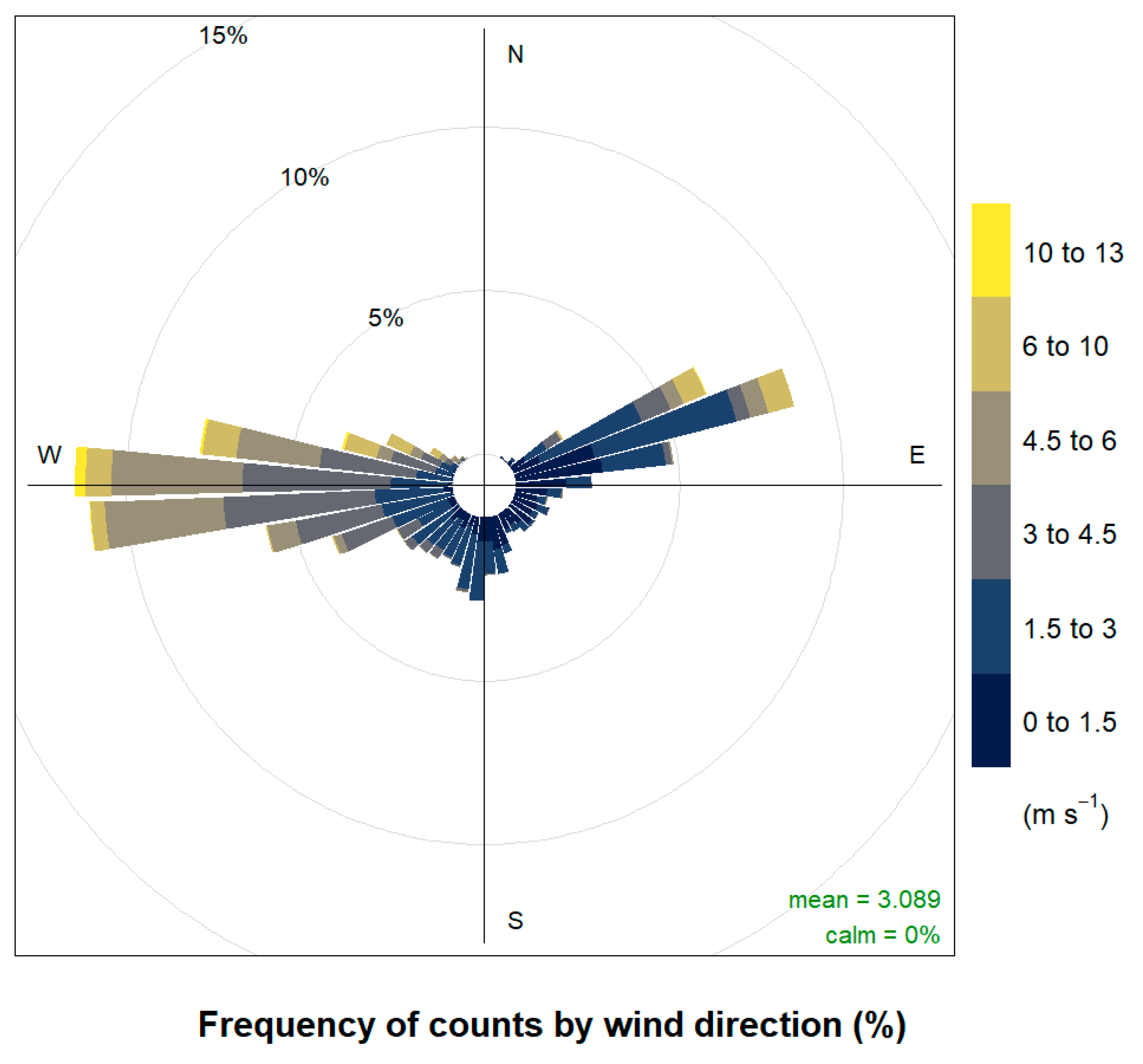
Figure 3.
Daily averages of greenhouse gas and aerosol parameters evaluated in this research study. A: Carbon monoxide (CO), in ppm (parts per million). B: Carbon dioxide (CO2), in ppm. C: Methane (CH4), in ppm. D: Equivalent black carbon (eBC), in μg/m3. E: Particulate matter (PM) in μg/m3, divided into the size ranges PM1, PM2.5, PM4, and PM10.
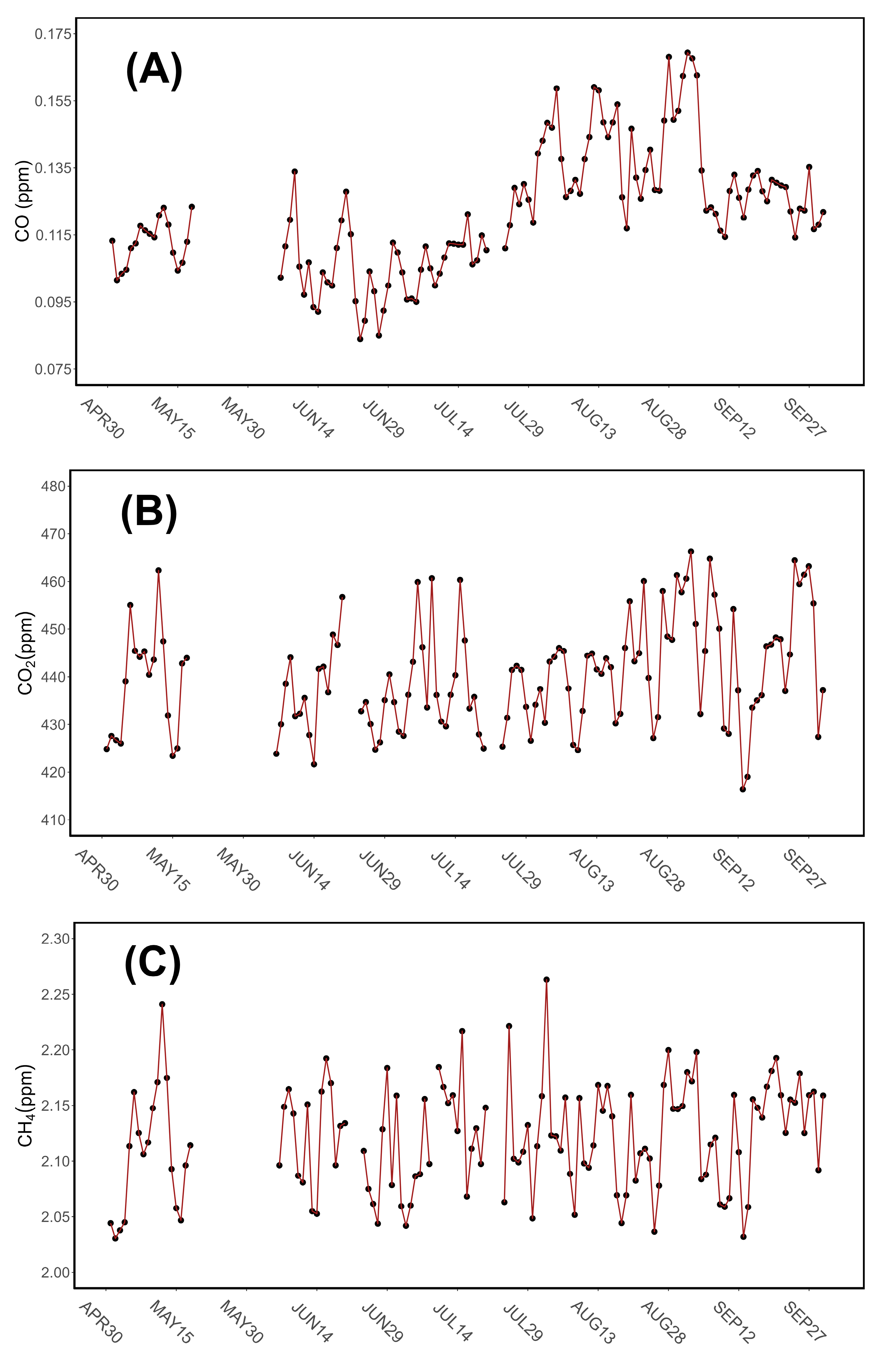
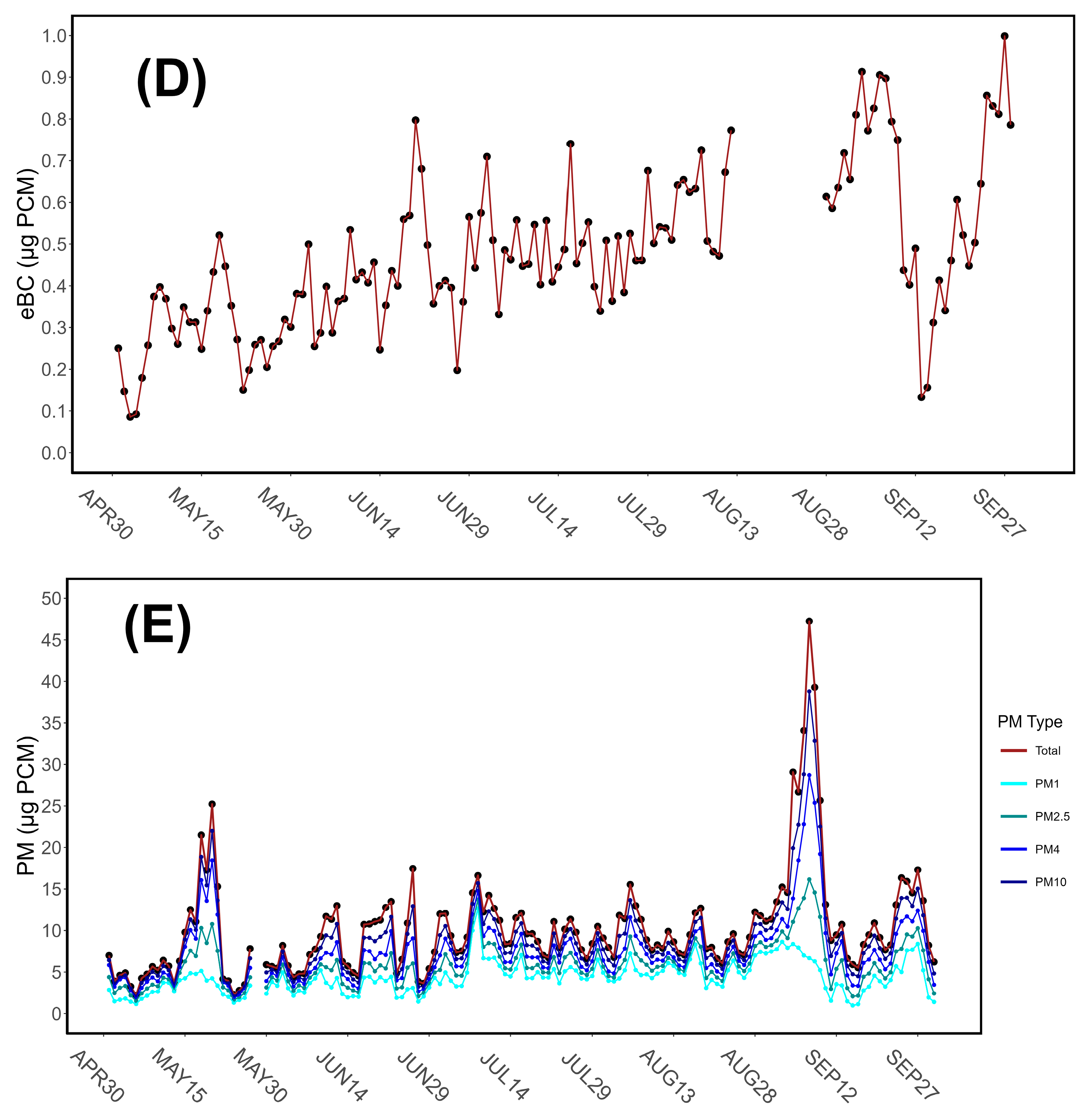
Figure 4.
Daily averages of environmental and meteorological data. A: Solar radiation in W/m2. B: Temperature, in Celsius degrees °C. C: Relative humidity, as percentage (%). D: SCA, as M/m.
Figure 4.
Daily averages of environmental and meteorological data. A: Solar radiation in W/m2. B: Temperature, in Celsius degrees °C. C: Relative humidity, as percentage (%). D: SCA, as M/m.
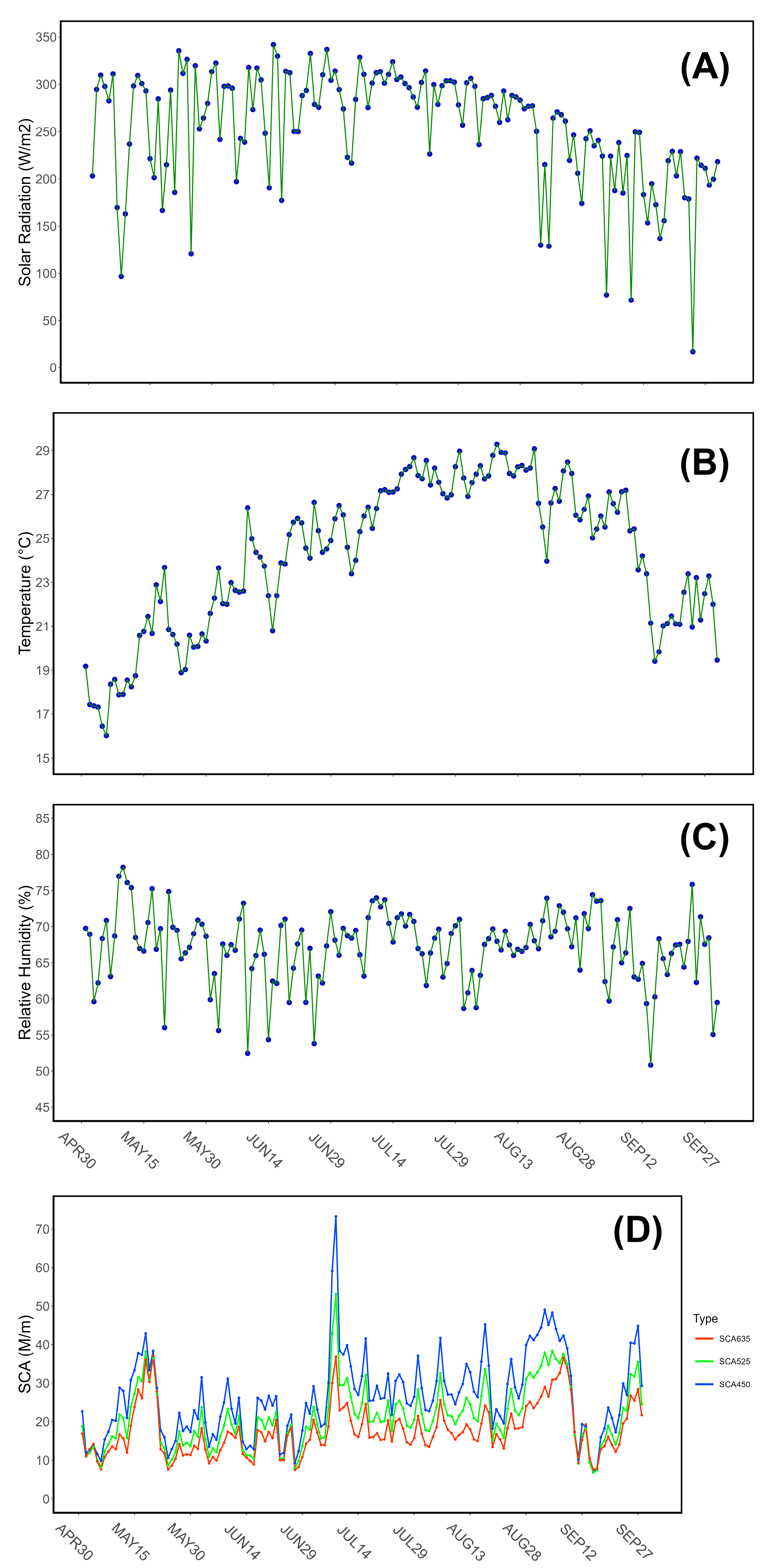
Figure 5.
Hourly averages of greenhouse gas and aerosol parameters evaluated in this research study. A: Carbon monoxide (CO), in ppm (parts per million). B: Carbon dioxide (CO2), in ppm. C: Methane (CH4), in ppm. D: Equivalent black carbon (eBC), in μg/m3. E: Particulate matter (PM) in μg/m3, divided into the size ranges PM1, PM2.5, PM4, and PM10.
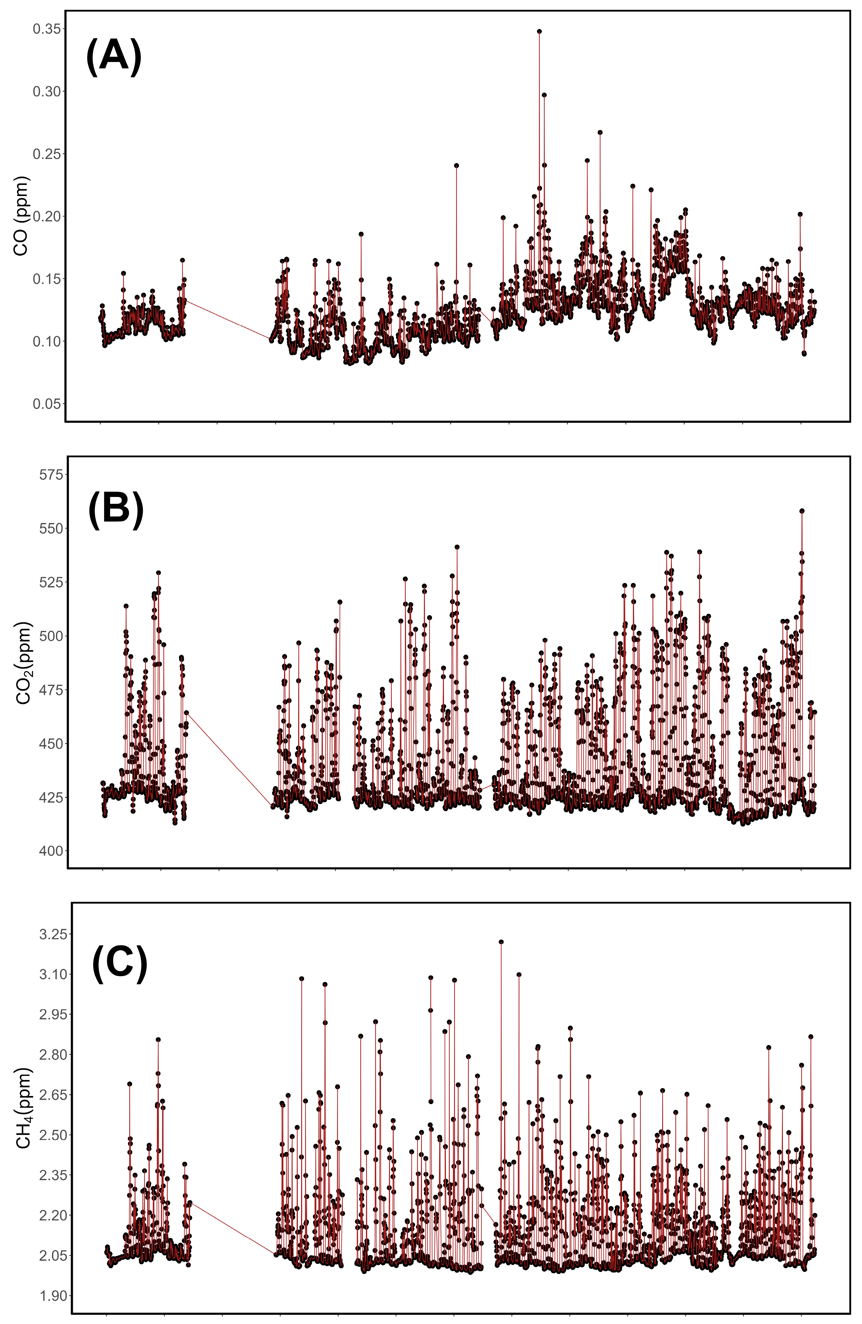
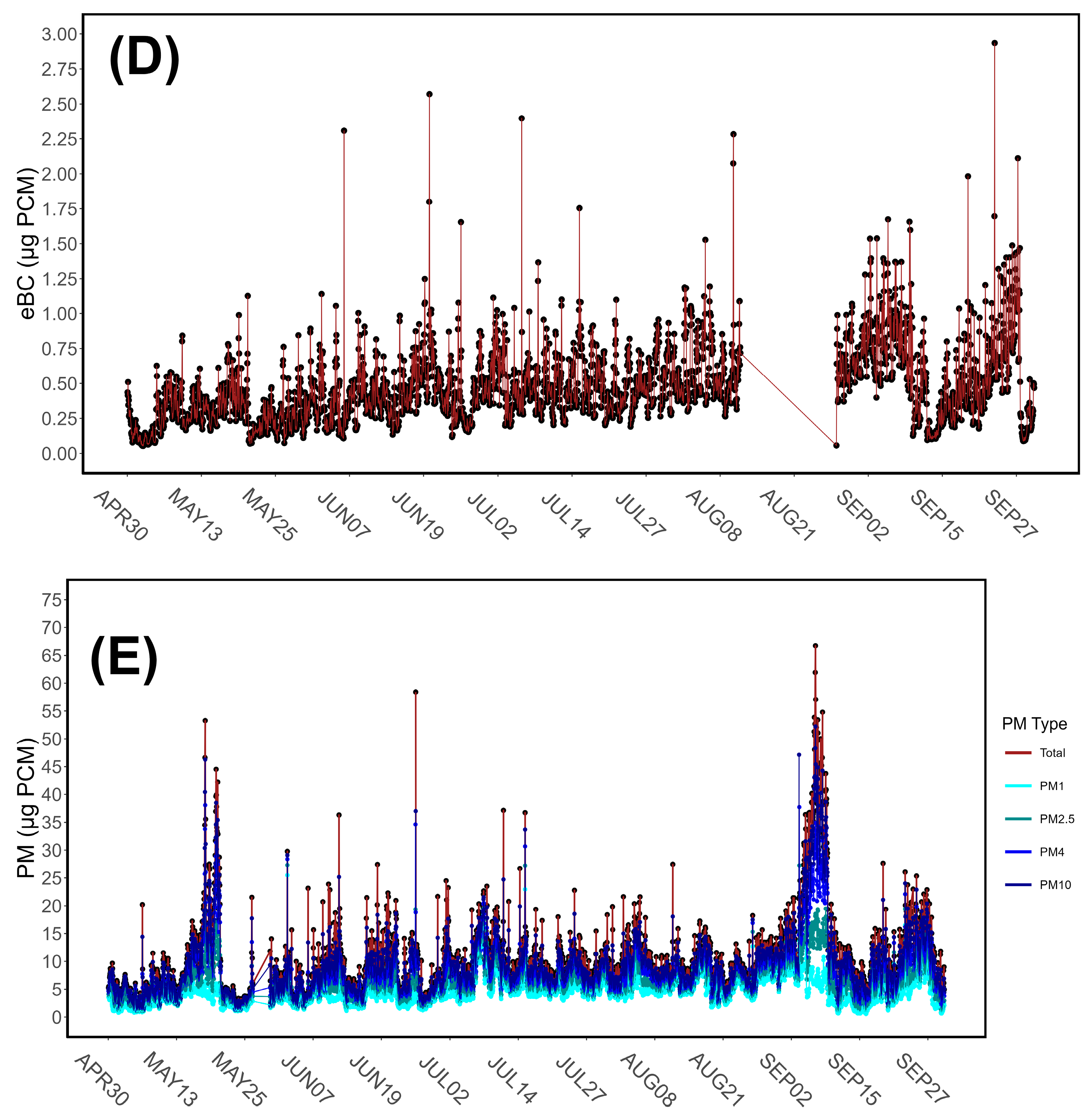
Figure 6.
Daily averages of environmental and meteorological data. A: Temperature, in Celsius degrees °C. B: Relative humidity, as percentage (%). C: SCA, as M/m.
Figure 6.
Daily averages of environmental and meteorological data. A: Temperature, in Celsius degrees °C. B: Relative humidity, as percentage (%). C: SCA, as M/m.
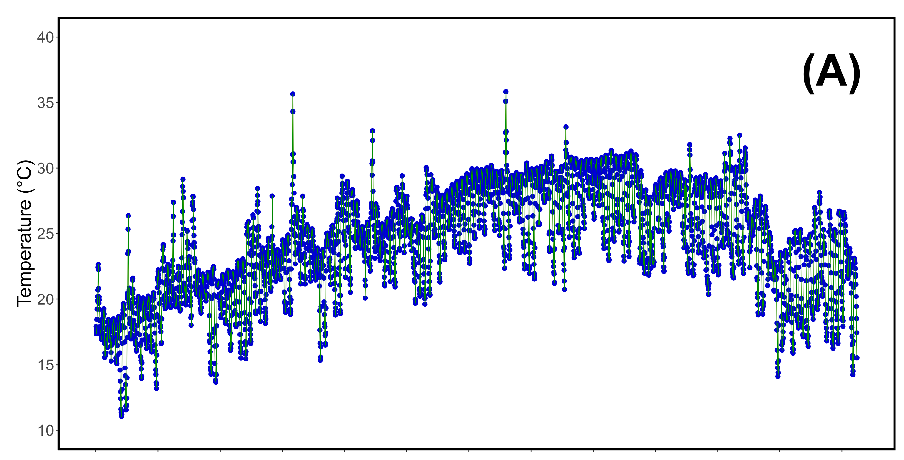
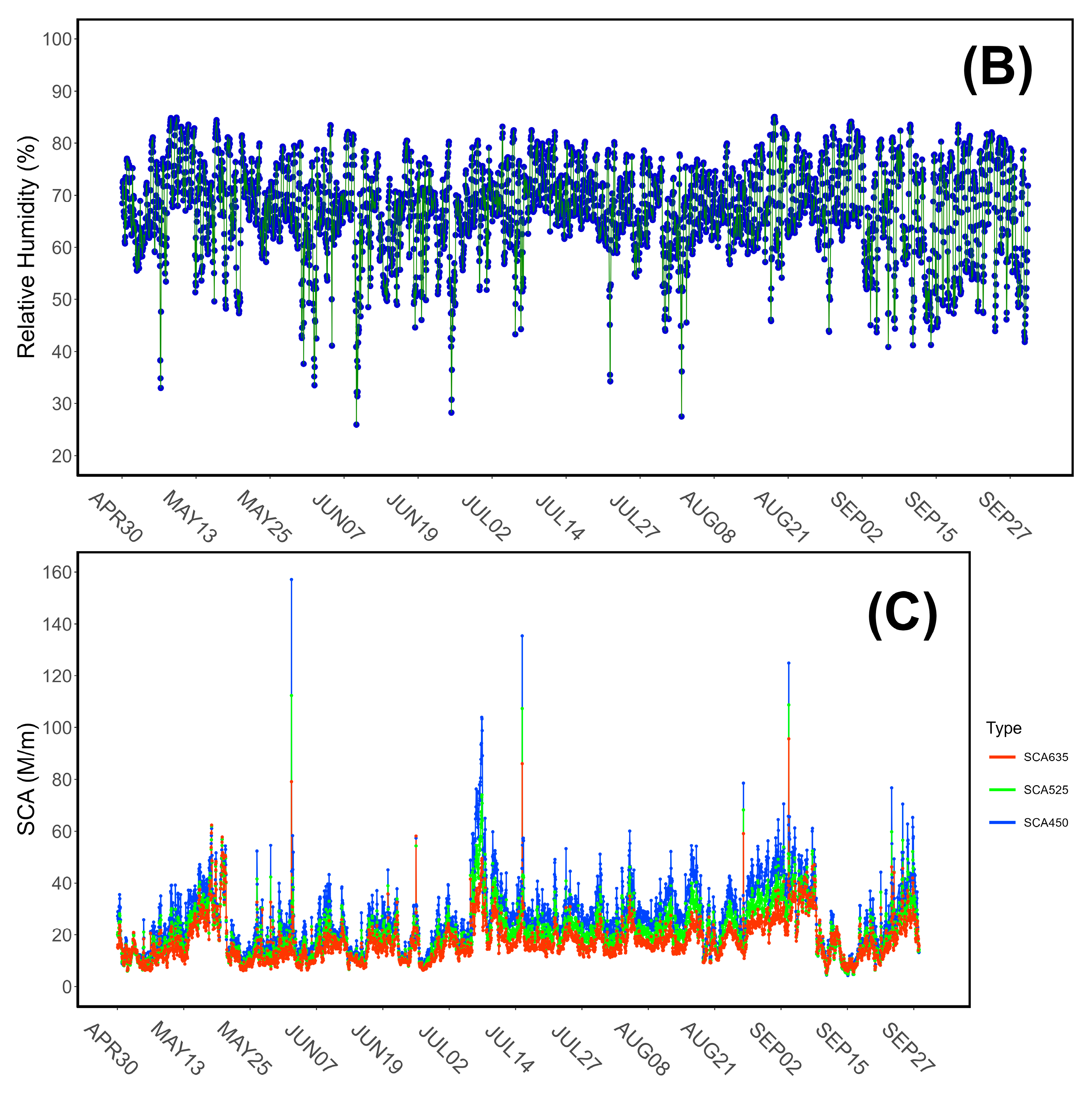
Figure 7.
Daily cycles of greenhouse gas and aerosol parameters analyzed in this research study, divided by wind regime. A: Carbon monoxide (CO), in ppm (parts per million). B: Carbon dioxide (CO2), in ppm. C: Methane (CH4), in ppm. D: Equivalent black carbon (eBC), in μg/m3. E: Particulate matter (PM) in μg/m3, divided into the size ranges PM1, PM2.5, PM4, and PM10 but not accounting for wind regime categories. F: PM2.5, with wind regimes. G: PM10, with wind regimes.
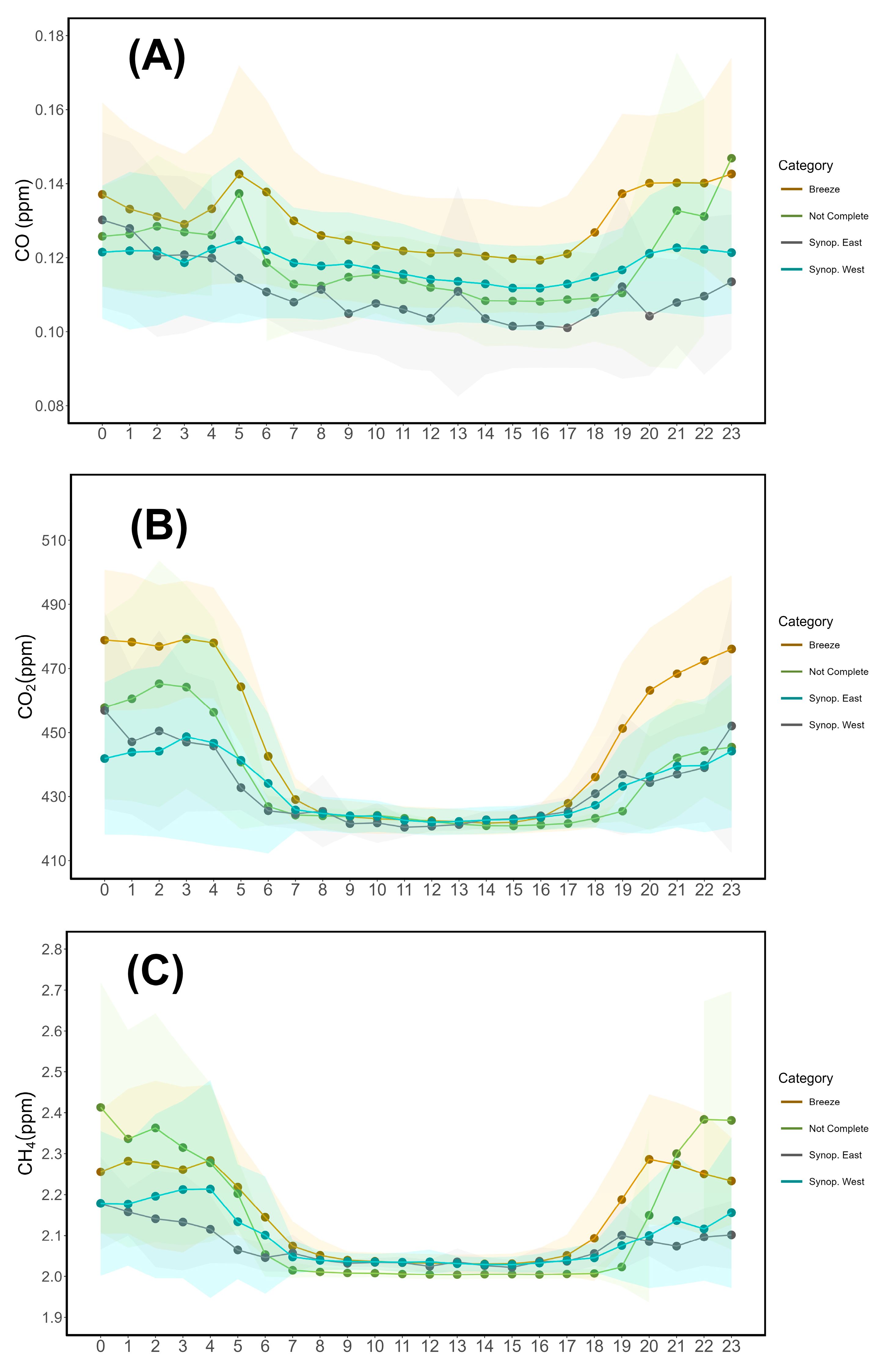
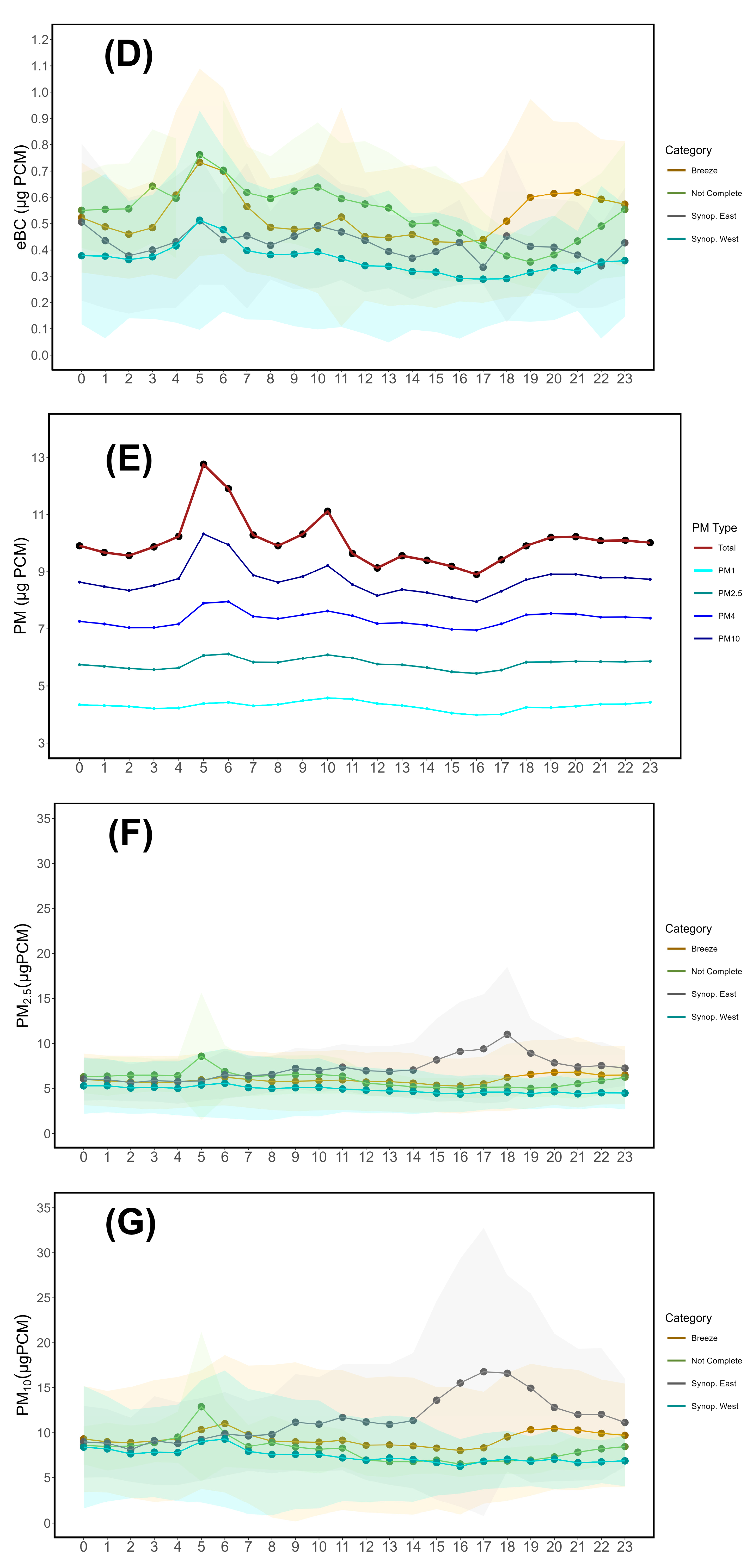
Figure 8.
Daily cycles of environmental and meteorological data. A: Temperature (°C). B: Relative humidity (%). C: SCA (M/m).
Figure 8.
Daily cycles of environmental and meteorological data. A: Temperature (°C). B: Relative humidity (%). C: SCA (M/m).
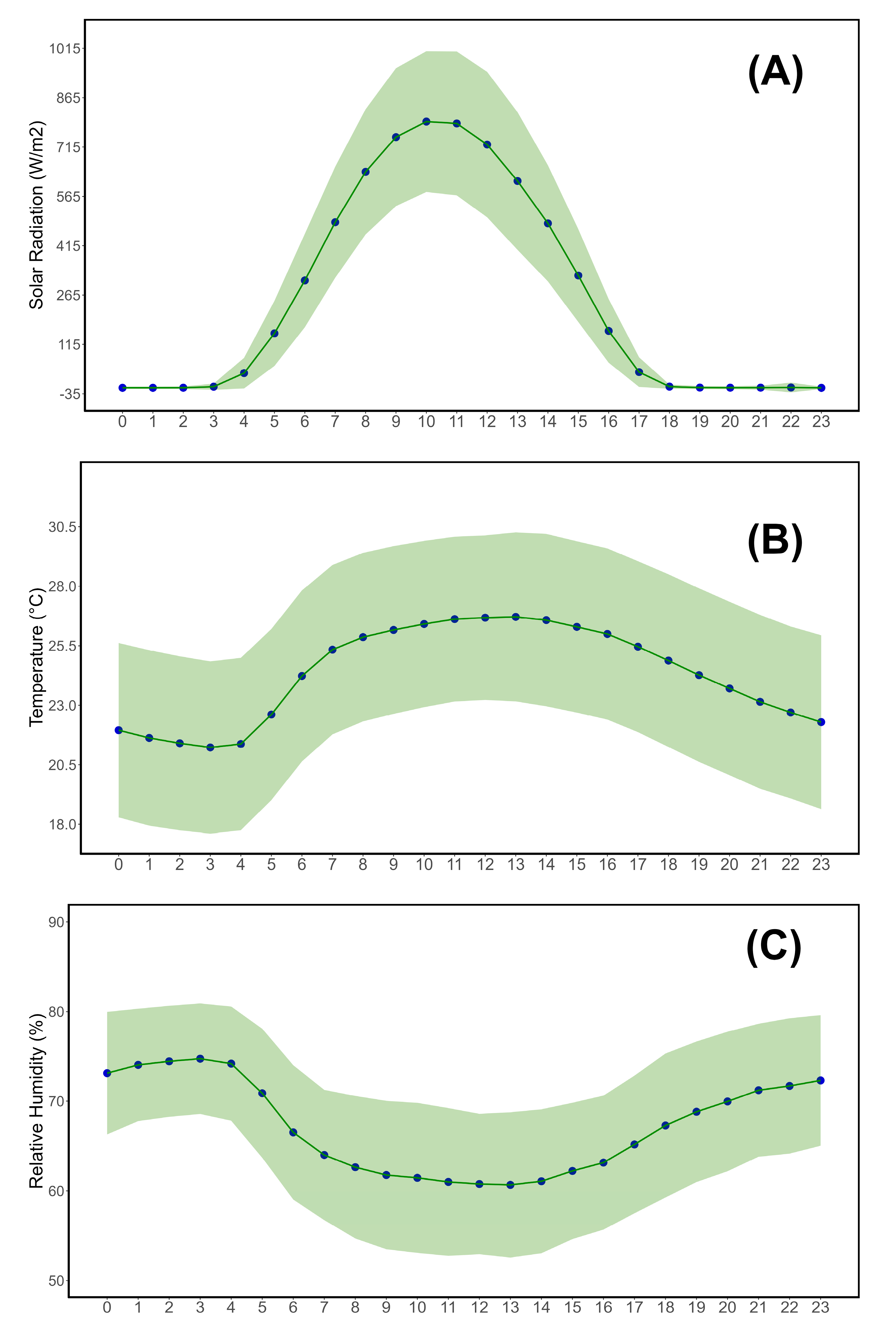
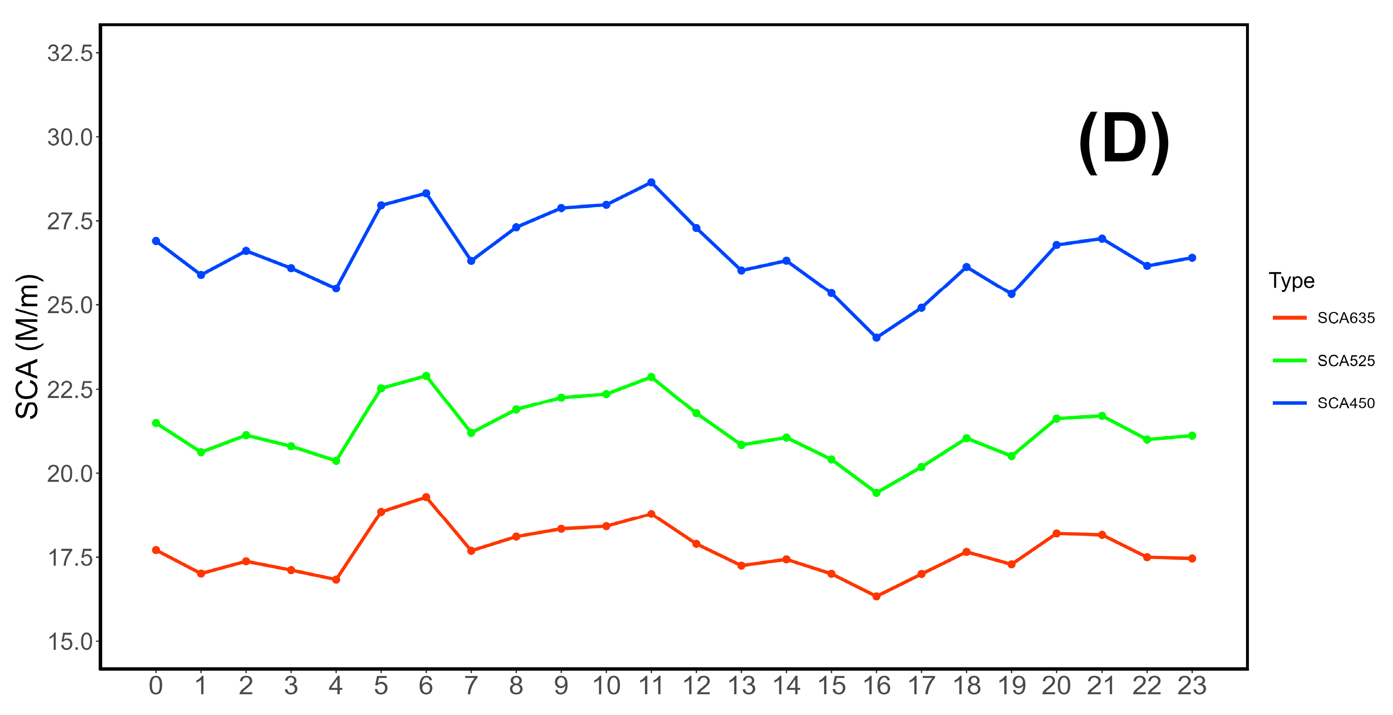
Figure 9.
Percentile roses of GHGs and aerosols evaluated in this study. The radius of each rose shows concentrations, while the shaded areas represent the coverage rate by percentile range. A: Carbon monoxide (CO). B: Carbon dioxide (CO2). C: Methane (CH4). D: Equivalent black carbon (eBC). E: Total particulate matter (PM). F: PM2.5. G: PM10.
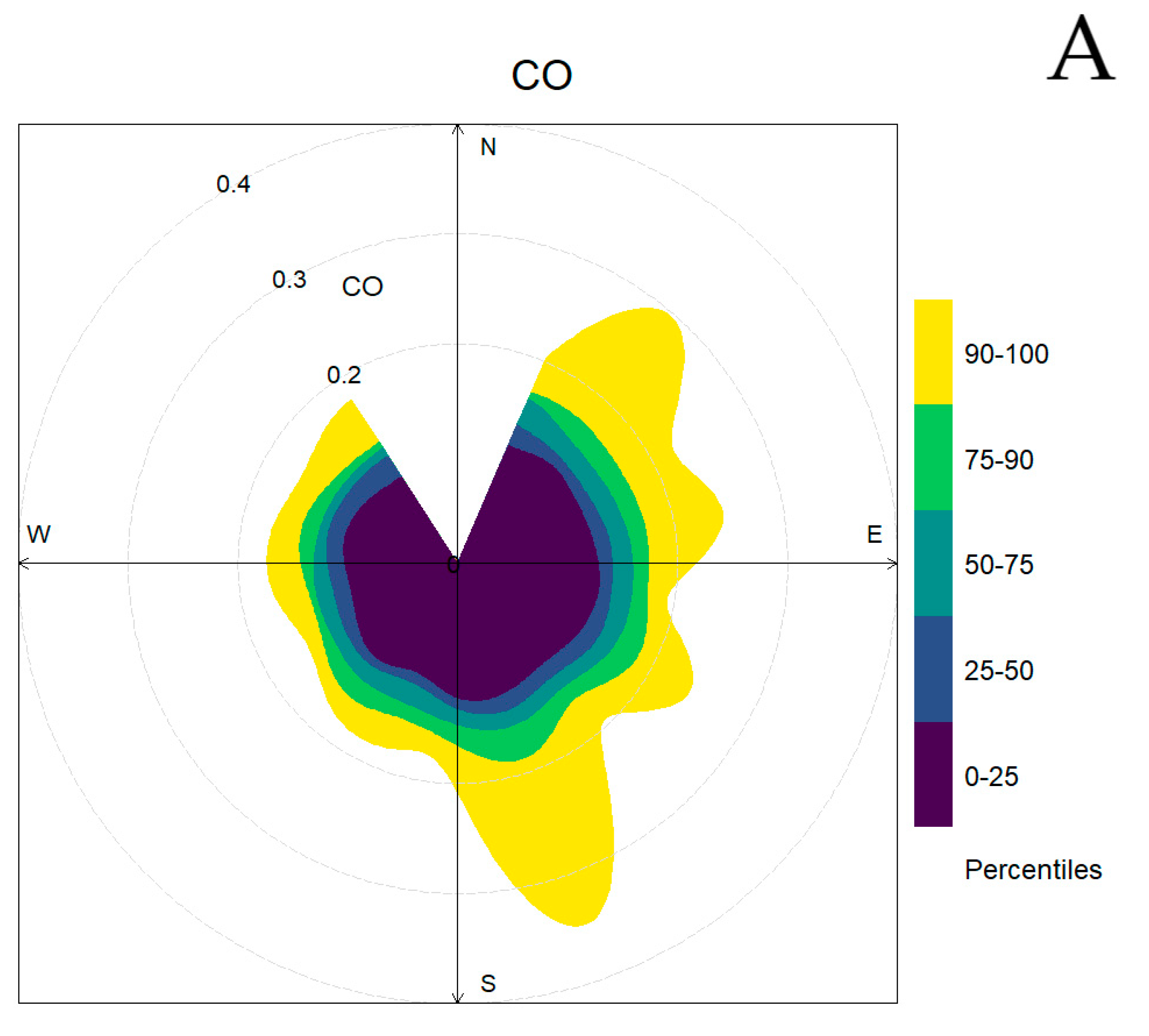
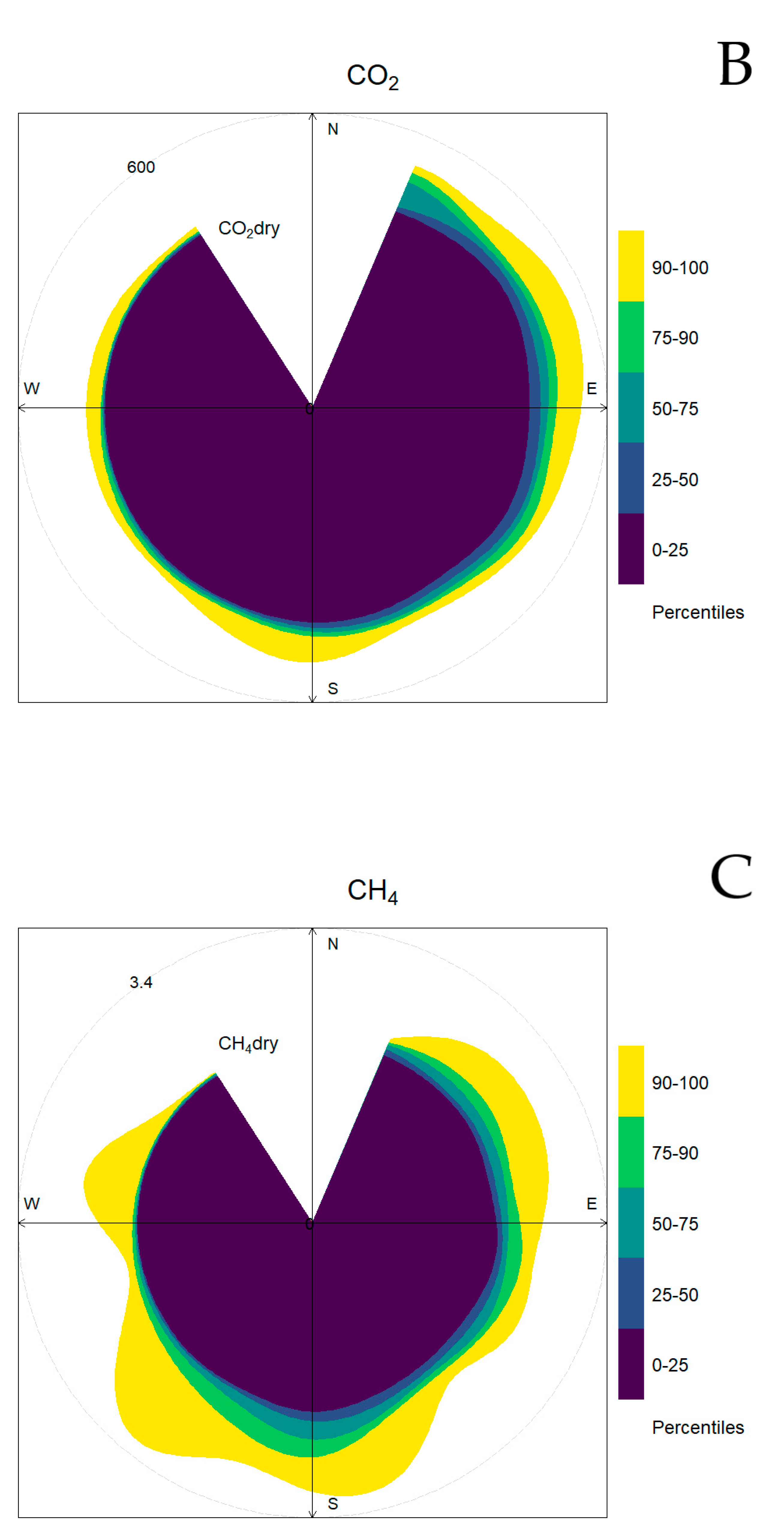
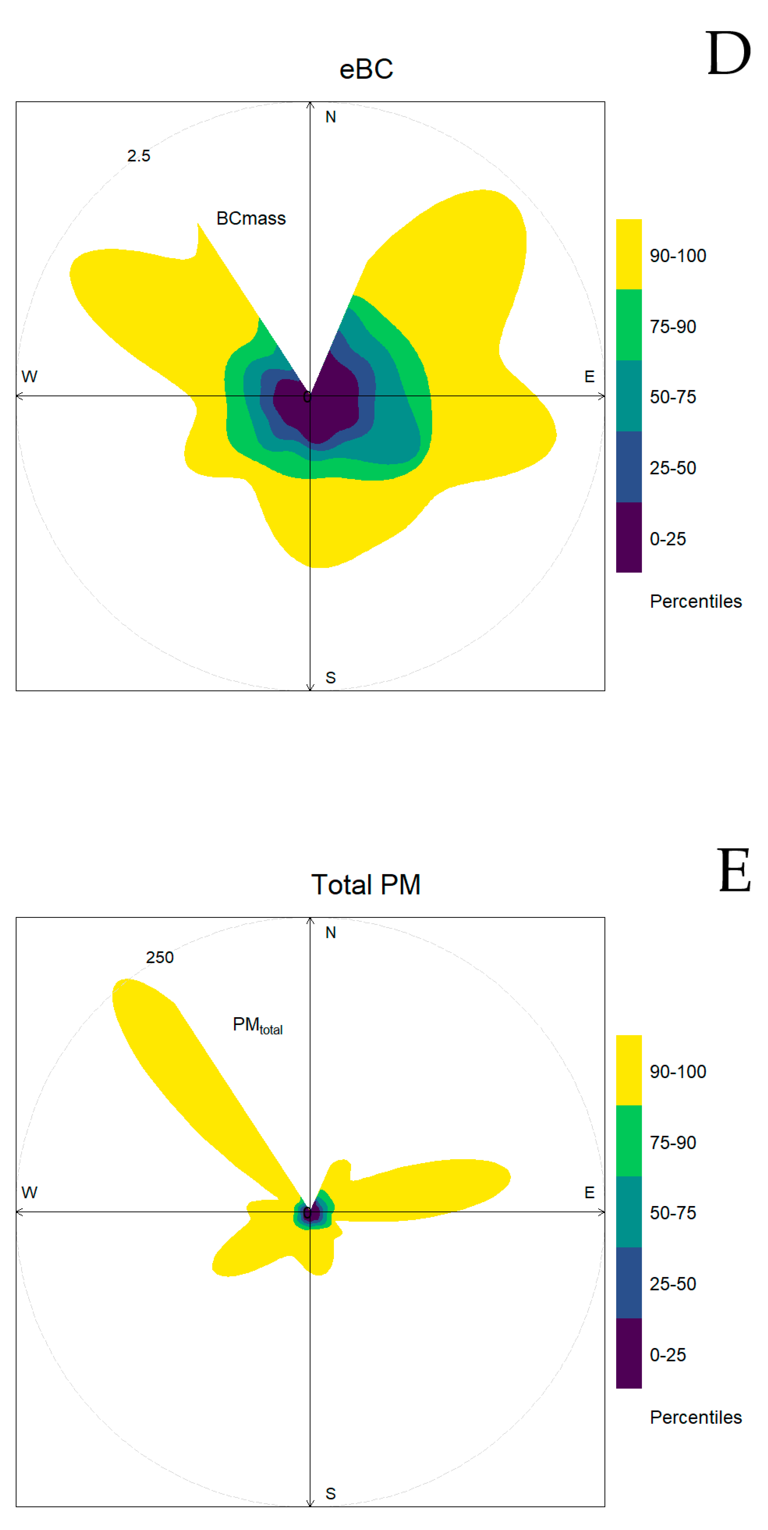
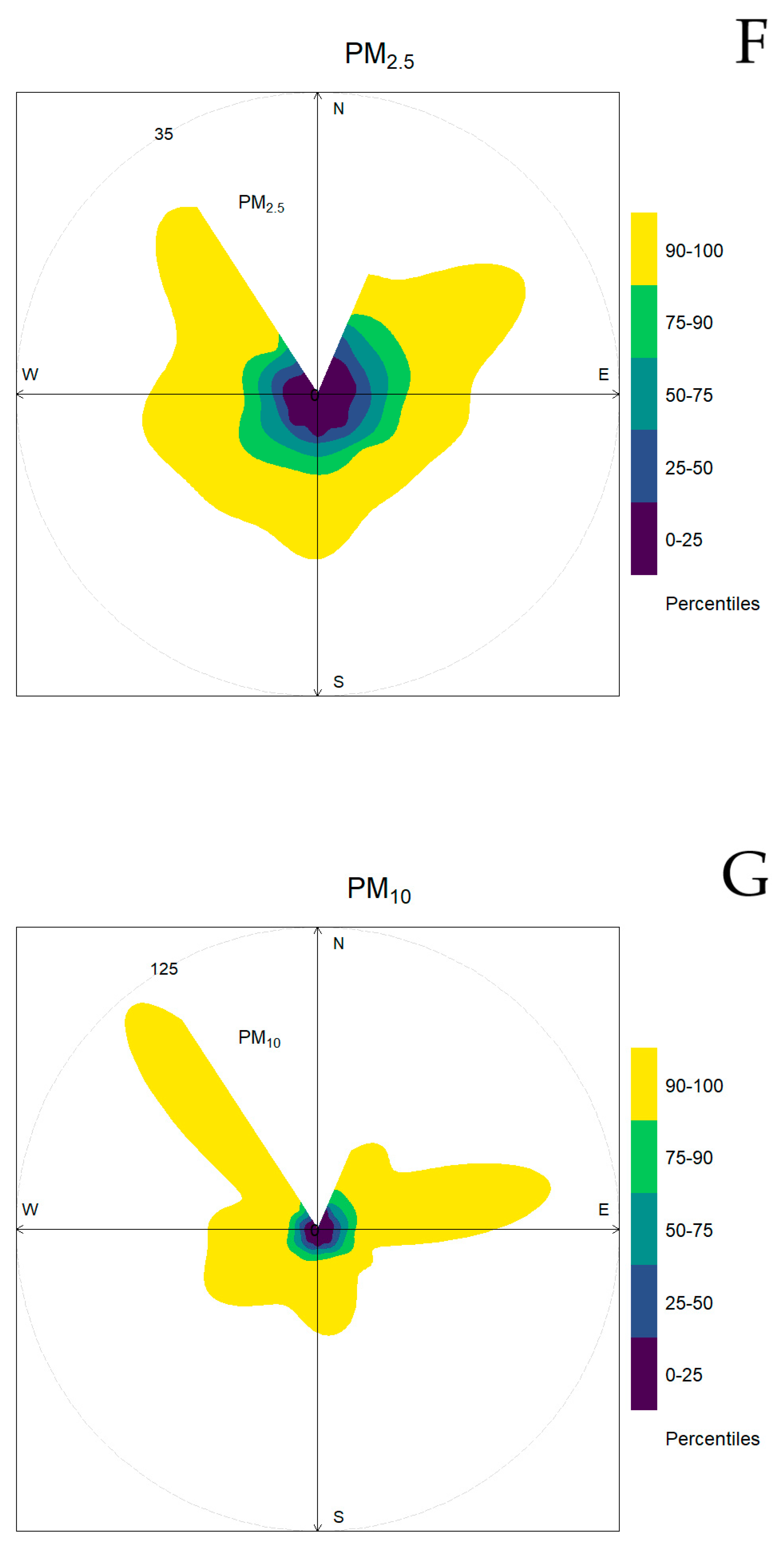
Figure 10.
Daily (A) and hourly (B) averages of PBLH at LMT. Daily cycle (C) divided by the four wind regime categories described in section 2.2.
Figure 10.
Daily (A) and hourly (B) averages of PBLH at LMT. Daily cycle (C) divided by the four wind regime categories described in section 2.2.
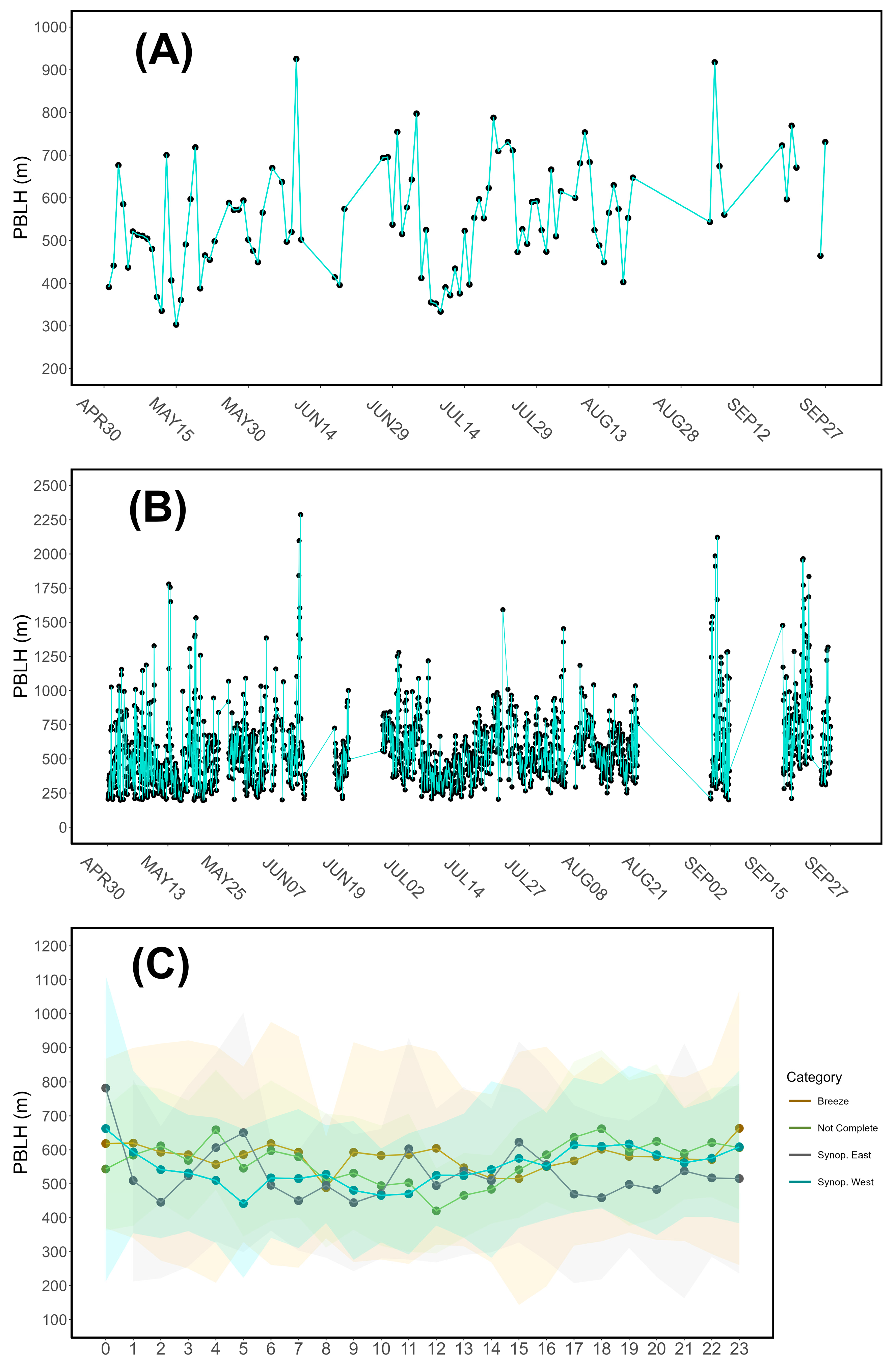
Figure 11.
Temporal variation of ceilometer backscattered profiles, aggregated on a 5-minute basis, during select days with synoptic flows from west (May 1st, 2nd) and east (May 14th, 15th), well-developed breeze (August 11th, 12th), and not complete breeze (July 17th, 18th).
Figure 11.
Temporal variation of ceilometer backscattered profiles, aggregated on a 5-minute basis, during select days with synoptic flows from west (May 1st, 2nd) and east (May 14th, 15th), well-developed breeze (August 11th, 12th), and not complete breeze (July 17th, 18th).
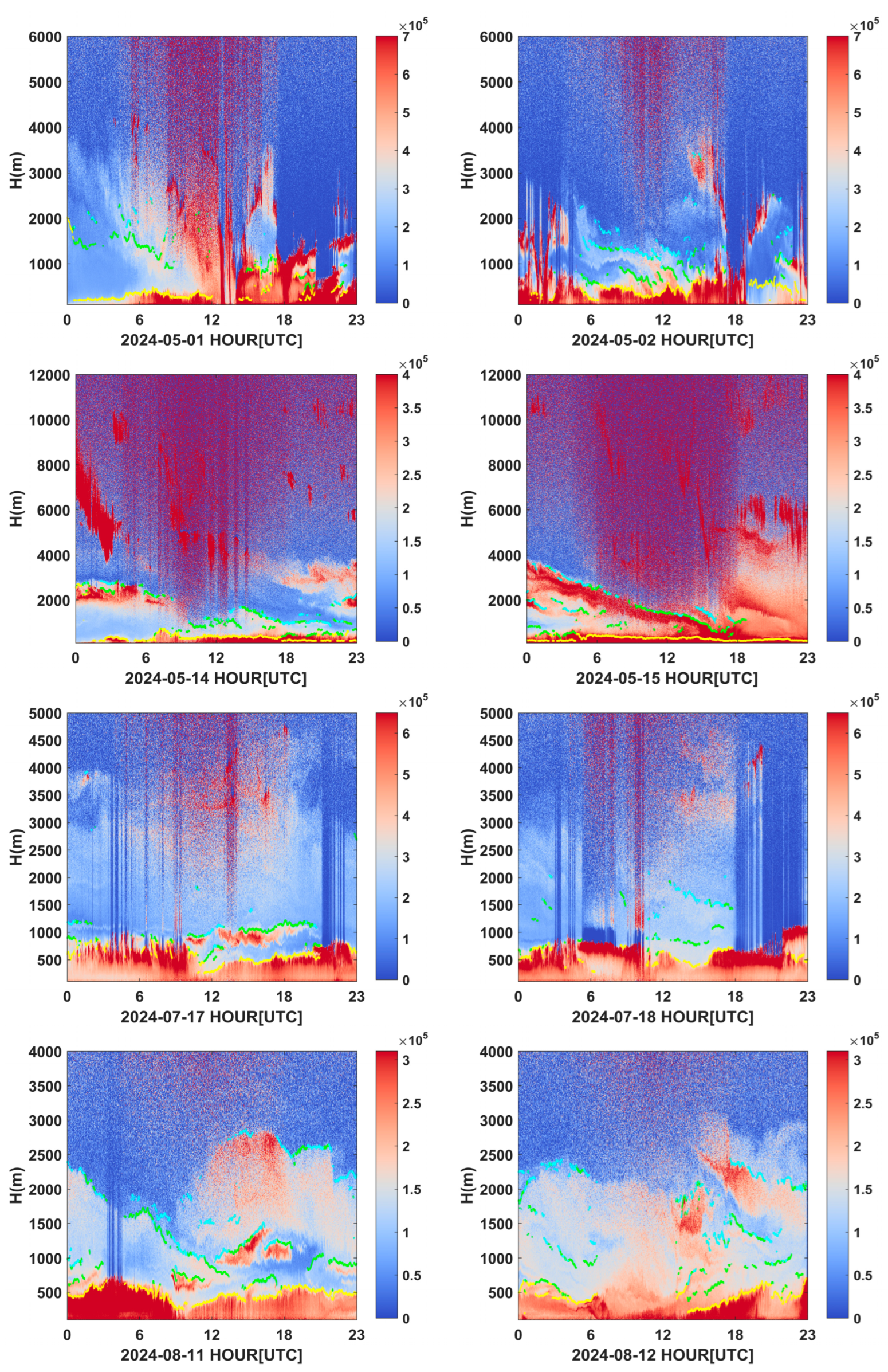
Figure 12.
Scatter and quantile-quantile plots between PBLH and carbon monoxide (CO) under the four observed wind regimes (top: breeze and not complete breeze; bottom: western and eastern synoptic flows).
Figure 12.
Scatter and quantile-quantile plots between PBLH and carbon monoxide (CO) under the four observed wind regimes (top: breeze and not complete breeze; bottom: western and eastern synoptic flows).
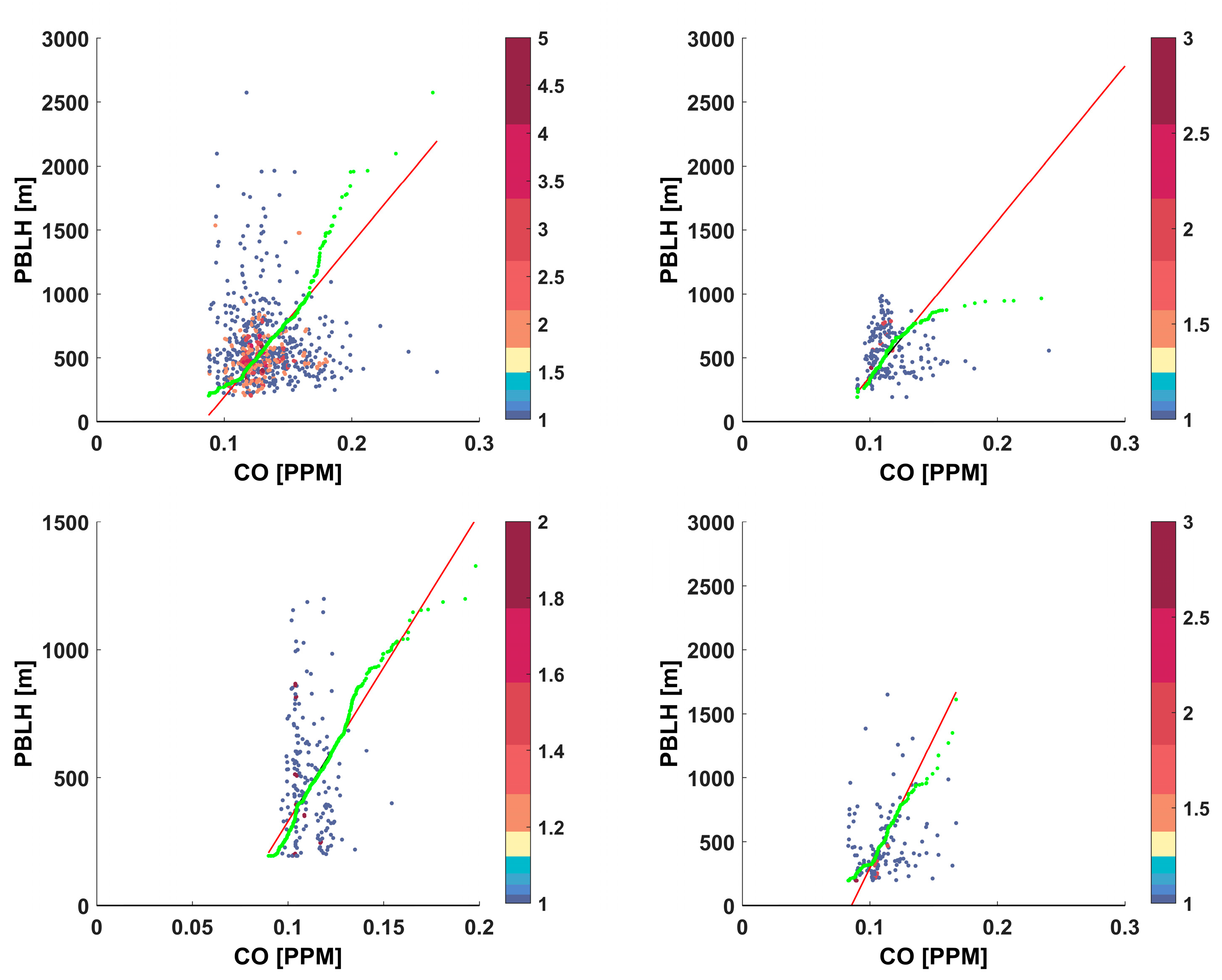
Figure 13.
Scatter and quantile-quantile plots between PBLH and carbon dioxide (CO2) under the four observed wind regimes (top: breeze and not complete breeze; bottom: western and eastern synoptic flows).
Figure 13.
Scatter and quantile-quantile plots between PBLH and carbon dioxide (CO2) under the four observed wind regimes (top: breeze and not complete breeze; bottom: western and eastern synoptic flows).
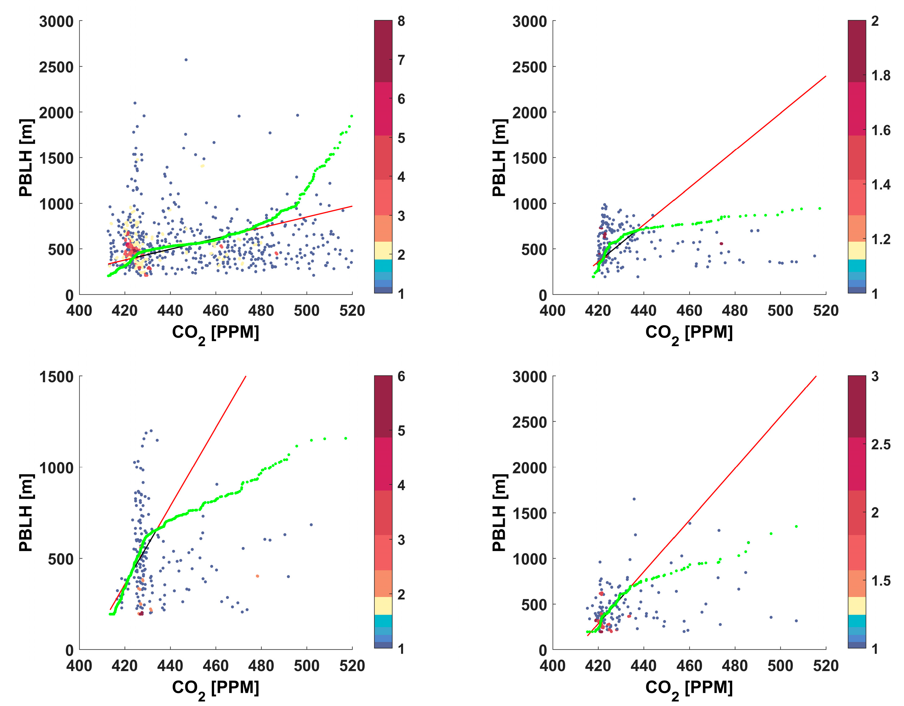
Figure 14.
Scatter and quantile-quantile plots between PBLH and methane (CH4) under the four observed wind regimes (top: breeze and not complete breeze; bottom: western and eastern synoptic flows).
Figure 14.
Scatter and quantile-quantile plots between PBLH and methane (CH4) under the four observed wind regimes (top: breeze and not complete breeze; bottom: western and eastern synoptic flows).
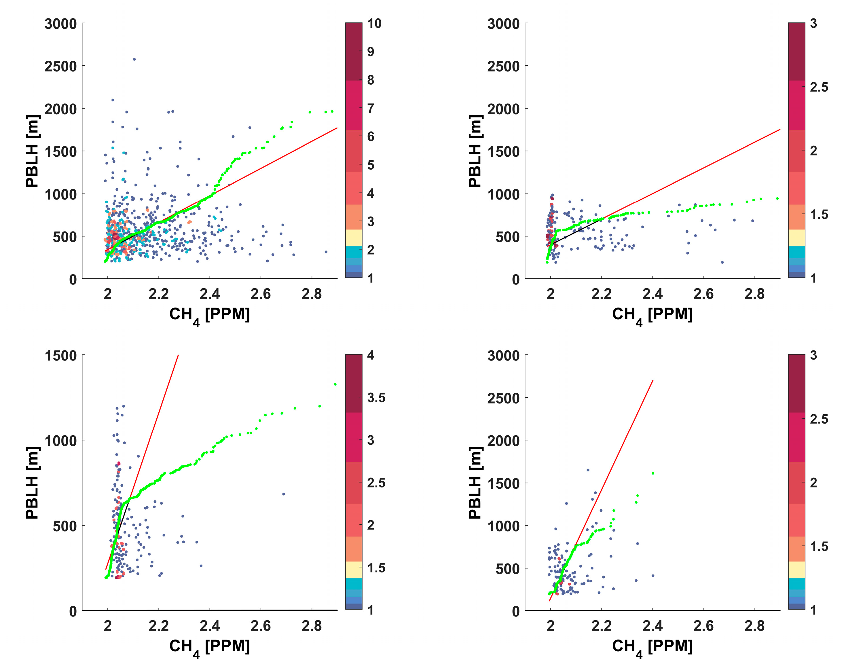
Figure 15.
Scatter and quantile-quantile plots between PBLH and equivalent black carbon (eBC) under the four observed wind regimes (top: breeze and not complete breeze; bottom: western and eastern synoptic flows).
Figure 15.
Scatter and quantile-quantile plots between PBLH and equivalent black carbon (eBC) under the four observed wind regimes (top: breeze and not complete breeze; bottom: western and eastern synoptic flows).
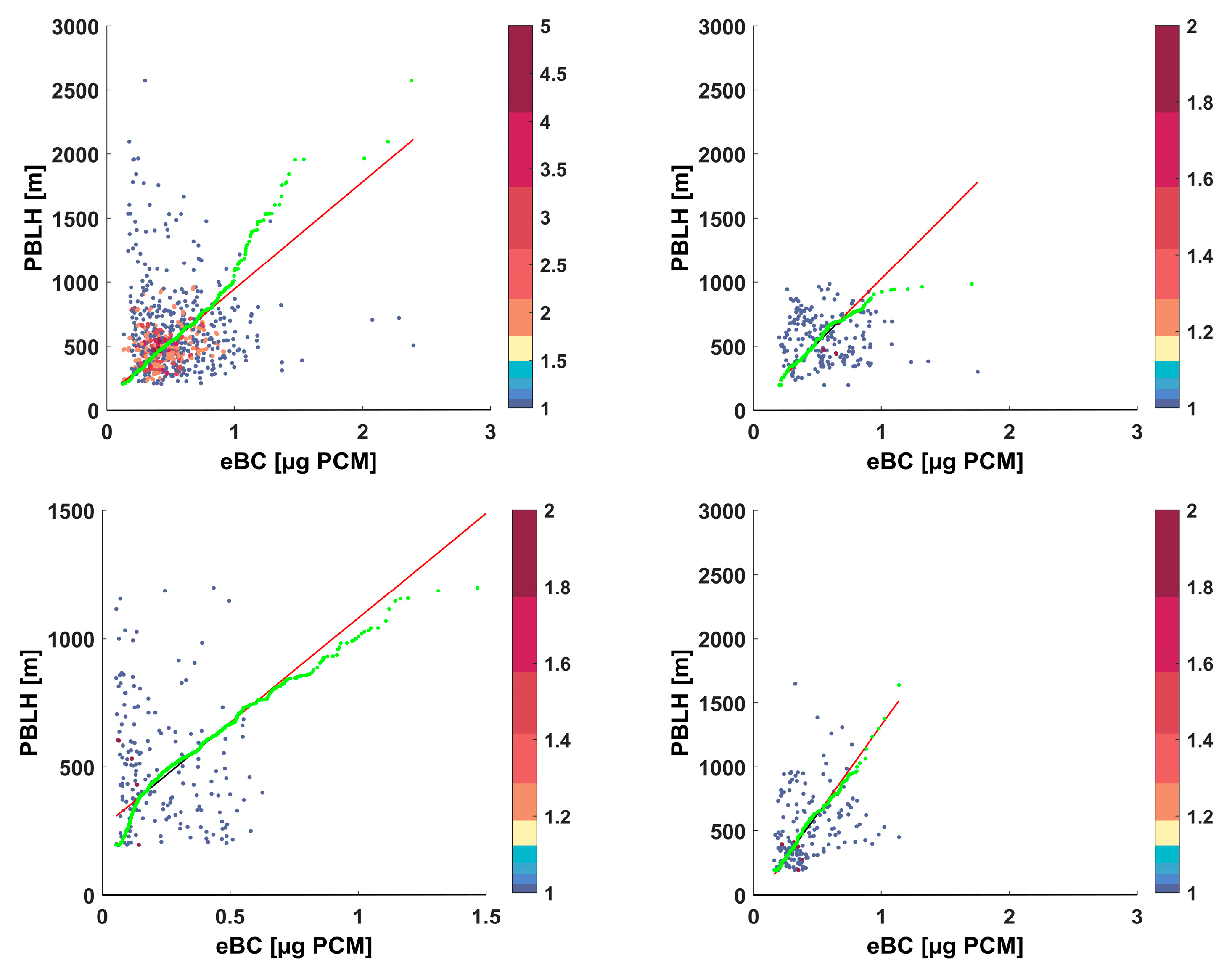
Figure 16.
Scatter and quantile-quantile plots between PBLH and PM2.5 under the four observed wind regimes (top: breeze and not complete breeze; bottom: western and eastern synoptic flows).
Figure 16.
Scatter and quantile-quantile plots between PBLH and PM2.5 under the four observed wind regimes (top: breeze and not complete breeze; bottom: western and eastern synoptic flows).
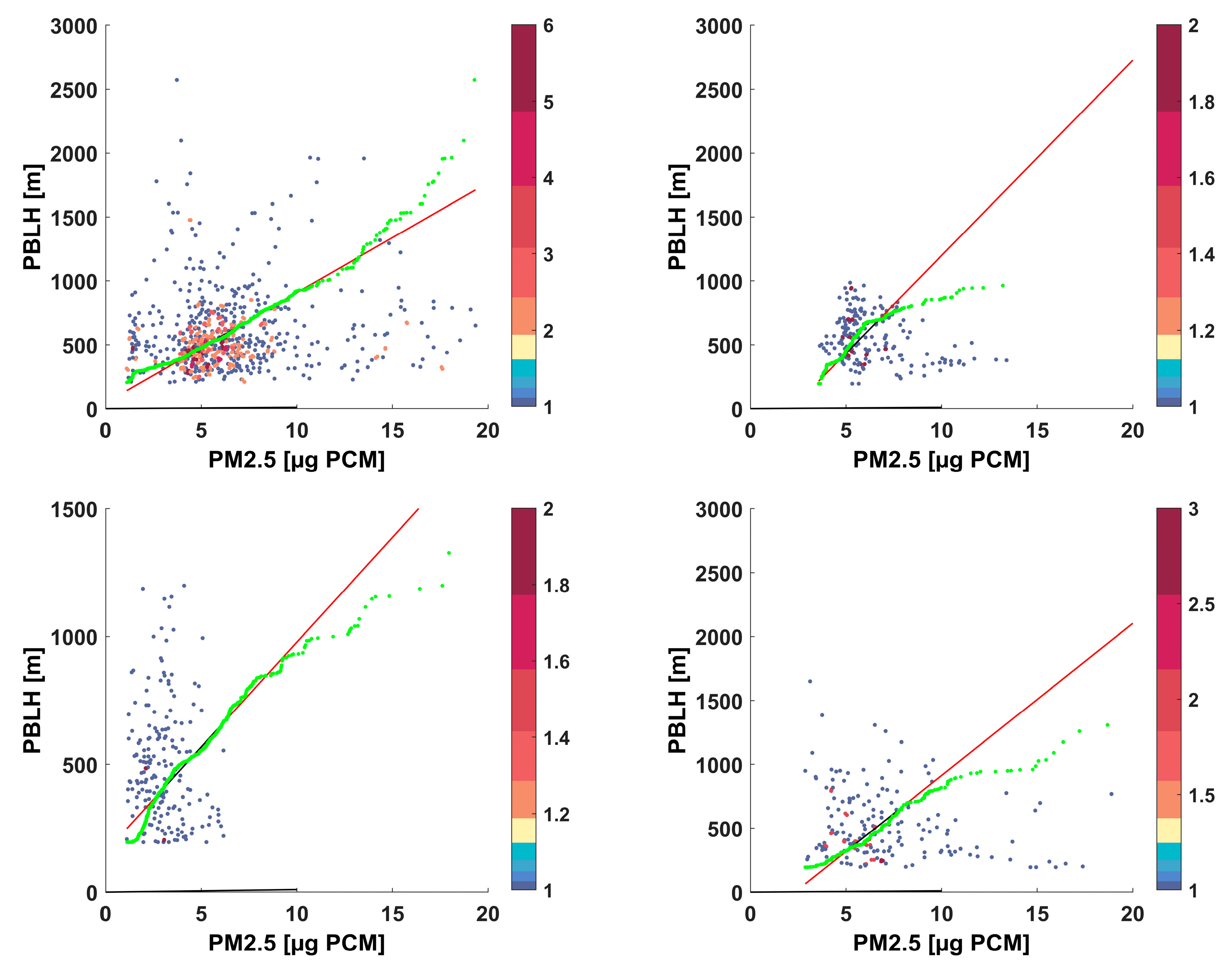
Figure 17.
Scatter and quantile-quantile plots between PBLH and PM10 under the four observed wind regimes (top: breeze and not complete breeze; bottom: western and eastern synoptic flows).
Figure 17.
Scatter and quantile-quantile plots between PBLH and PM10 under the four observed wind regimes (top: breeze and not complete breeze; bottom: western and eastern synoptic flows).
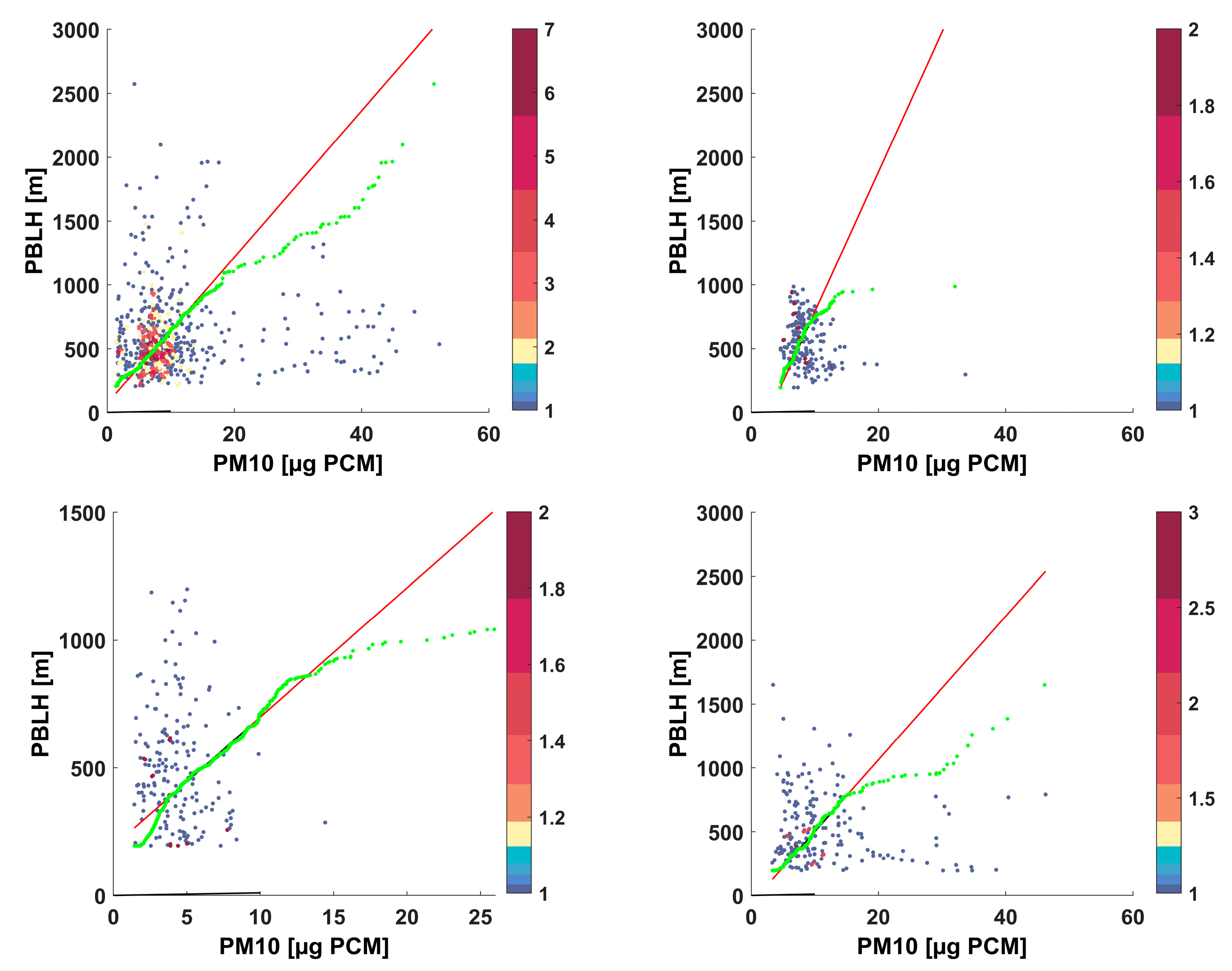

Table 1.
Technical specifications of the Lufft CHM 15k Nimbus ceilometer.
| Parameters | Description / Values |
|---|---|
| Laser source | Nd: YAG solid-state laser |
| Wavelength | 1064 nm |
| Operating mode | Pulsed |
| Pulse energy | 7 µJ |
| Pulse repetition frequency | 5–7 kHz |
| Filter bandwidth | 1 nm |
| Field of view receiver | 0.45 mrad |
Table 2.
Dataset coverage as percentage (%) of the total number of days and hours.
| Type | G2401 | MAAP | Fidas | WXT520 | Nimbus |
|---|---|---|---|---|---|
| Days | 86.27% | 88.88% | 98.69% | 100% | 66.66% |
| Hours | 81.26 % | 89.1% | 97.76% | 99.7% | 59.47% |
Table 3.
Number of days, per month, falling into each of the four wind regime categories.
| Months | East. Synoptic | West. Synoptic | Breeze | NC Breeze |
|---|---|---|---|---|
| May | 4 | 15 | 1 | 0 |
| June | 1 | 2 | 5 | 0 |
| July | 2 | 4 | 8 | 8 |
| August | 1 | 5 | 8 | 2 |
| September | 0 | 7 | 17 | 0 |
Disclaimer/Publisher’s Note: The statements, opinions and data contained in all publications are solely those of the individual author(s) and contributor(s) and not of MDPI and/or the editor(s). MDPI and/or the editor(s) disclaim responsibility for any injury to people or property resulting from any ideas, methods, instructions or products referred to in the content. |
© 2024 by the authors. Licensee MDPI, Basel, Switzerland. This article is an open access article distributed under the terms and conditions of the Creative Commons Attribution (CC BY) license (http://creativecommons.org/licenses/by/4.0/).
Copyright: This open access article is published under a Creative Commons CC BY 4.0 license, which permit the free download, distribution, and reuse, provided that the author and preprint are cited in any reuse.


