
Submitted:
12 June 2025
Posted:
17 June 2025
You are already at the latest version
Abstract
Gaseous pollutants and aerosols resulting from anthropic activities and natural phenomena require adequate source apportionment methodologies to be fully assessed. Furthermore, it is crucial to differentiate between fresh anthropogenic emissions and the atmospheric background. The Proximity method based on the O3/NOx (ozone to nitrogen oxides) ratio has been used at the Lamezia Terme (code: LMT) World Meteorological Organization – Global Atmosphere Watch (WMO/GAW) regional station in Italy to determine the variability of CO (carbon monoxide), CO2 (carbon dioxide), CH4 (methane), SO2 (sulfur dioxide), and eBC (equivalent black carbon), thus allowing to differentiate local and remote sources of emission. Prior to this work, all O3/NOx ratios lower than 10 were grouped under the LOC (local) proximity category, thus including very low ratios (≤ 1) which are generally attributed by literature to “urban” air masses, particularly enriched in anthropogenic emissions. This study introduces the URB category in the assessment of CO, CO2, CH4, SO2, and eBC variability at the LMT site, highlighting patterns and peaks in concentrations that were previously neglected. The daily cycle, which is locally influenced by wind circulation and Planetary Boundary Layer (PBL) dynamics, is particularly susceptible to urban-scale emissions and its analysis has allowed to highlight notable peaks in concentrations that were previously neglected. Correlations with wind corridors and speeds indicate that most evaluated parameters are linked to northeastern winds at LMT and wind speeds under 5.5 m/s. Weekly cycle analyses, i.e. differences between weekdays (MON-FRI) and weekends (SAT-SUN) has also highlighted tendencies driven by seasonality and wind corridors. The results highlight the potential of the URB category as a tool necessary to access a given area’s anthropogenic output and its impact on air quality and the environment.
Keywords:
sulfur dioxide
; equivalent black carbon
; tropospheric ozone
; nitrogen oxides
; Lamezia Terme
; Mediterranean Basin
; air mass aging
; proximity indicator
; proximity progression factor
1. Introduction
The variability of greenhouse gases (GHGs), aerosols, reactive gases, and other components of Earth’s atmosphere requires advanced methodologies to be fully assessed [1,2,3,4,5,6,7,8]. Defining short term (e.g., seasonal) and long term trends is necessary for policymakers and regulators to mitigate emissions and reduce the impact of anthropogenic climate change [9,10,11,12].
Many pollutants are both natural and anthropic in origin, and require source apportionment techniques to be evaluated. Via a number of methodologies, such as the study of stable carbon isotopes, it is possible to discriminate anthropogenic emissions from their natural counterparts [13,14,15]. The findings of Parrish et al. [16] and Morgan et al. [17] showed the potential of the O3/NOx ratio (ozone to nitrogen oxides) as an air mass aging and proximity indicator. Higher ratios (>100) are representative of the atmospheric background, while lower ratios (<10) indicate fresh air masses enriched in anthropogenic pollutants. Intermediate ratios are representative of the transition between near sources/outflows and remote sources/outflow.
Prior to these findings, a study by Steinbacher et al. [18] highlighted the possible overestimation of NO2 concentrations by instruments relying on heated molybdenum converters; with NOx being the result of NO + NO2, air mass aging categories based on the O3/NOx ratio would therefore be affected by these issues. In literature, there are several reports concerning the issue of measuring “true NOx” [19,20,21,22,23,24]. At the Lamezia Terme (code: LMT) WMO/GAW (World Meteorological Organization – Global Atmosphere Watch) regional station in Italy, a correction factor of 0.5 was implemented to account for the possible overestimation of NO2; this correction was applied to preliminary data gathered at the station [25], and – consequently – to nine years (2015-2023) of data to evaluate in greater detail the local variability of greenhouse gases [26].
While the NO2 overestimation is instrumental in nature, a second correction factor was applied at LMT [26] to account for peaks in photochemical activity and the consequent overproduction of near-surface O3, observed in particular from diurnal winds in the direction of the Tyrrhenian Sea during the Spring and Summer seasons [27,28].
Previous studies have allowed to determine peculiar behaviors in the variability of a number of gases (CO: carbon monoxide; CO2: carbon dioxide; CH4: methane; SO2: sulfur dioxide) [26,29] and aerosols (eBC: equivalent black carbon) [29], thus demonstrating the potential of this methodology in source apportionment efforts. In fact, these parameters are characterized by different atmospheric lifetimes [30,31,32,33,34,35], as well as the coexistence of anthropogenic and natural sources which require precise source apportionment to be differentiated [36,37,38,39,40,41,42,43,44,45,46,47]. Additionally, these parameters have different global trends, where for instance CO2 [48,49,50,51] and CH4 [42,52,53] are on the increase while SO2 has a generally decreasing trend due to optimized combustion engines and fuels [54,55,56,57], however volcanic eruptions can result in notable SO2 emissions in the atmosphere, thus affecting global tendencies [58,59,60]. Mount Pinatubo’s eruption of 1991 [61] and the The Hunga Tonga–Hunga Haʻapai eruption of 2022 [62,63] have been subject to numerous studies aimed at assessing the effects of volcanic eruptions on global scales. CO is characterized by years of decline, followed by an upward trend attributed to wildfire emissions [64] and changes in emission mitigation policies [65,66]. BC also shows a decline linked to emission mitigation policies, however punctual peaks linked to wildfires occur and affect not only air quality [67], but also climate balances [68,69].
At LMT, all parameters with the exception of SO2 showed gradual reductions in concentrations in the transition from the LOC (local) category to BKG (atmospheric background), consistent with anthropic influences: SO2’s behavior, with the intermediate N–SRC (near source) and R–SRC (remote source) categories generally yielding higher concentrations than LOC and BKG, have allowed – combined with previous assessments of SO2 sources of emission on a regional scale [70] – to provide a degree of spatial resolution to proximity categories [29], as they were more qualitative in nature [16,17].
All previous studies on LMT data based on the O3/NOx ratio grouped values lower than 10 to the LOC category; however, the leading literature on the method attributes ratios lower than 1, i.e. with a higher number of NOx molar fractions compared to O3, to “urban” air masses, deemed particularly enriched in pollutants linked to anthropic activities [16,17]. Prior to this study, the urban (“URB”) category has never been considered not only at LMT, but also in the broader context of the national atmospheric observation network. This study is therefore aimed at introducing URB to evaluate in detail local anthropogenic sources of emissions and test a number of hypotheses raised by previous studies at LMT.
This work is organized as follows: in Section 2, the LMT site – also accounting for local orography and its impact on local wind circulation – as well as employed instruments and methodologies are described; the results are presented in Section 3; Section 4 and Section 5 discuss the results and conclude the paper, respectively.
2. The WMO/GAW Observation Site, Measured Data, and Methodologies
2.1. Characteristics of the Lamezia Terme (LMT) WMO/GAW Station
The LMT observation site is located in the southern Italian region of Calabria (Lat: 38.8763 °N; Lon: 16.2322 °E; Elev: 6 meters above sea level) (Figure 1A), in the central Mediterranean Basin. Operated by the National Research Council of Italy – Institute of Atmospheric Sciences and Climate (CNR-ISAC), LMT has been gathering data for the WMO/GAW (World Meteorological Organization – Global Atmosphere Watch) network since 2015.
The station is 600 meters from the Tyrrhenian coast, in the westernmost sector of the Catanzaro Isthmus, which is the narrowest point in the entire Italian peninsula (Figure 1B). In the isthmus, the distance between the Tyrrhenian and the Ionian (eastern) coasts of Calabria is approximately 32 kilometers, thus resulting in a peculiar orographic configuration in the country. The isthmus separates two mountain ranges in the north, the Coastal Chain (Catena Costiera) and the Sila Massif, from the southern Serre Massif. Local geomorphology is heavily influenced by plate tectonics, with intense faulting being responsible for the current configuration of the isthmus and variations in elevation across the area [71,72,73,74]. During the early Quaternary, the Catanzaro isthmus was a tidal strait connecting the Tyrrhenian and Ionian seas, as evidenced by the findings of 2D and 3D dunes in outcrops located in the central sector of the isthmus itself [75,76,77]. Consequently, changes in sea level driven by the uplift of Calabria [78,79,80] and the transition between glacial and interglacial periods [81,82] have cut off the sea passage, thus resulting in the present-day configuration. The area is subject to intense faulting and seismic activity [83], with many of the strongest earthquakes (three out of ten with Mw ≥ 6.95) in recorded Italian history having their estimated epicenters within ≈20 kilometers from the current location of LMT, according to the national inventory [84,85].
The present-day configuration of the isthmus has a notable effect on near-surface wind circulation, as shown by a study on ten years of LMT wind profiles [86]. Local wind circulation also affects air traffic, as the Lamezia Terme International Airport (IATA: SUF; ICAO: LICA) located 3 kilometers north of LMT has a 10/28 (100/280 °N) runway (RWY) orientation, reflecting the same patterns observed at LMT.
The Marcellinara Gap (Sella di Marcellinara) located in the middle area of the isthmus results in northeastern winds being channeled in the direction of LMT (Figure 1B), as evidenced by early studies on wind circulation [87,88]. Near-surface wind circulation is dominated by breeze regimes and is oriented on a well-defined W-WSW/NE-ENE axis, however when the 850 hPa layer is considered, NW winds prevail in accordance with large scale circulation in the area [87]. From March to October, local and large-scale flows combine and dominate diurnal breezes; the November to February period is characterized by diurnal circulation more closely connected to large-scale forcing [88].
In addition to wind circulation patterns and profiles [89,90], over time multiple studies have assessed the variability of gases and aerosols at the site [91]. Preliminary findings on reactive gas and CH4 variability were first described in Cristofanelli et al. [25], including the first implementation of the O3/NOx ratio methodology. In this study, local air masses were found to be particularly enriched in CH4, thus indicating nearby sources of emission such as livestock farming. Another study, based on seven years of measurements (2016-2022), allowed to evaluate the variability of CH4 with greater detail, especially with respect to wind circulation and seasonality [92]. Northeastern-continental winds were found to be generally enriched in CH4, while western-seaside winds generally yielded lower concentrations. Wintertime concentrations were higher compared to their summertime counterparts, and similarly, nighttime concentrations were found to be significantly higher than daytime molar fractions, reflecting the influence of wind circulation on local measurements. Additionally, in the northeastern wind sector, low wind speeds were linked to high concentrations and, vice versa, high speeds were linked to lower concentrations: this behavior was described as HBP (Hyperbola Branch Pattern) in the same study.
These features were not reported for surface O3, which showed the opposite pattern in a study based on nine years (2015-2023) of measurements: at LMT, O3 peaks during diurnal hours from the western-seaside sector [27], a finding that resulted in the introduction of the “enhanced correction” (ecor) for the O3/NOx ratio methodology (see Section 2.2). Another study demonstrated that O3 peaks, which are a key indicator of regional photochemical pollution, were linked to precise combinations of temperature, wind direction/speed, and downward solar radiation [28].
Due to its location in the central Mediterranean Basin, the LMT station is exposed to Saharan intrusions from Africa [93] and wildfire emissions at various scales [94]. In particular, during the 2021 wildfire crisis, peaks in CO and eBC were attributed, using multiple methodologies, to regional Calabrian [95] and Algerian/Greek wildfires [96]. Local wind patterns and precipitation phenomena linked to inversion between wind corridors allowed to observe wildfire outputs that would have otherwise been subject to air mass transport at higher altitudes.
2.2. Gas/Aerosol Datasets, and Employed Methodologies
In order to evaluate CO, CO2, CH4, SO2, and eBC using the Proximity methodology based on the O3/NOx ratio, multiple instruments have been used at LMT.
CO, CO2, and CH4 concentrations have been measured, between 2015 and 2023, by a Picarro G2401 (Santa Clara, California, USA) CRDS (Cavity Ring-Down Spectrometry) [97,98,99] analyzer. CRDS analyzers allow to gather data concerning the molar fractions of gaseous compounds up to the ppb (parts per billion) level. Measurements are performed every five seconds, and the outputs are aggregated on a hourly basis; although all measurements are in ppm (parts per million), CO and CH4 are converted in ppb due to their lower concentrations compared to CO2. These measurements are available from 2015 onwards. More information concerning these measurements is available in Malacaria et al. [91].
SO2 concentrations have been measured by a Thermo Scientific 32i (Franklin, Massachusetts, USA) instrument, whose principle of operation is based on UV (ultraviolet) light absorption of SO2 molecules. The instrument performs ten measurements per minute, used to generate hourly aggregates in ppb. These measurements are available from 2016 onwards. More details on T32i measurements at LMT are available in a previous study [70].
eBC [100] measurements at the site have been performed by a Thermo Scientific 5012 (Franklin, Massachusetts, USA) MAAP (Multi-Angle Absorption Photometer) [101,102]. The instrument relies on the short-wave absorption of BC and the measurement of the absorption coefficient at 637 nanometers. Measurements are performed every minute, and the outputs are aggregated on hourly data of micrograms per cubic meter (µg/m3). These measurements are available from 2016 onwards. Additional details concerning eBC measurements at LMT are available in previous research [95,103].
Thermo Scientific 49i (Franklin, Massachusetts, USA) and Thermo Scientific 42i-TL (Franklin, Massachusetts, USA) have been used to measure O3 and NOx at the site, respectively. Details concerning these instruments’ principles of operation and procedures are available in previous studies (O3: [25,27]; NOx: [25,104]).
All results have been integrated with meteorological data concerning wind speed and directions, which have been gathered by a Vaisala WXT520 (Vantaa, Finland) weather station or mast. The instrument, which also provides data on relative humidity, air pressure, precipitation, and hail, is positioned at an elevation of 10 meters above sea level. Wind direction and speed are measured, on a per-minute basis, by calculating the deviations of travel times of ultrasound pulses between transducers placed on a plane. Additional information on LMT’s mast measurements are available in previous studies [91,92,104].
In this study, the main air mass aging and proximity categories are used, with the implementation of URB for O3/NOx ratios lower or equal than 1. With this implementation, the LOC category which once accounted for all ratios ≤ 10, is now limited to the 1-10 range. Changes in the distribution of hourly data of the LOC category, based on the implementation of URB, are shown in Table 1. N–SRC (10-50), R–SRC (50-100), and BKG (> 100) are not affected in this study and detailed assessments concerning the variability of measured parameters under these categories are available in previous research [26,29].
Seasons are defined as per the following trimesters: DJF for Winter (December, January, February); MAM for Spring (March, April, May); JJA for Summer (June, July, August); SON for Fall (September, October, November). Wind corridors at LMT are defined based on previous research [26,27,28,70,92,104]: a range of 0–90 °N identifies the northeastern-continental sector, while 240–300 °N is used for the western-seaside sector.
The Proximity methodology is affected by well-known limitations, as its implementation is susceptible to instrumental availability and maintenance issues. Multiple instruments need to operate at the same time to attribute measurements to air mass aging categories, thus resulting in data loss. Table 2 (COx, CH4), Table 3 (SO2), and Table 4 (eBC) show the coverage rates, divided by year, of all measurements. “MTO” datasets integrate Vaisala WXT520 data on wind parameters, while “Prox” refer to hourly data for which a proximity category could be defined, i.e. data with valid O3 and NOx measurements. “MTOProx” combines the two subcategories, resulting in lower rates.
All hourly data used in this research have been processed and in R 4.4.2 using the dplyr, ggpubr, ggplot2, zoo, and tidyverse packages, also including their respective libraries.
3. Results
3.1. URB Category Concentrations
Previous studies provided average concentrations for each proximity category from LOC to BKG concerning CO, CO2, CH4 [26], SO2, and eBC [29]. In this work, the results include the new URB category, with the results being shown in Table 5 (CO, CO2, CH4) and Table 6 (SO2, eBC), and Figure 2. Due to the relevant influence of local wind circulation on LMT’s measurements, wind corridors and their respective concentrations are also reported.
Kruskal-Wallis tests [105] have been performed in R to assess the statistical significance of the differences between proximity categories, also accounting for wind corridors. All tests provided very significant results (p-values < 2.2×10⁻¹⁶). A pairwise Wilcoxon (or Mann-Whitney U) test [106,107] was performed to verify the statistical significance of differences between each pair of proximity categories using the Bonferroni correction [108,109]: all results are very significant (p-values <<< 0.01), with the exception of SO2 which yielded URB/LOC (p = 0.0029, still significant), URB/R–SRC (p = 0.0898, not significant), and LOC/BKG (p = 0.0052, still significant).
Concentrations for each proximity category have also been calculated on a seasonal basis, with the results shown in Figure 3. For the URB and LOC categories, the statistical significance of the averages reported for all seasons have been tested using the Kruskal-Wallis test [105]. All results are statistically very significant (p-values <<< 0.01).
Using the Wilcoxon test [106,107] with Bonferroni correction [108,109], all results based on pairs of two seasons have yielded statistically significant results, with the exception, for the URB category, of CO (Summer-Fall, p = 1), CH4 (Spring-Fall, p = 0.20; Winter-Spring, p = 0.40; Winter-Summer, p = 1; Spring-Summer, p = 1), SO2 (Spring-Fall, p = 0.13; Winter-Fall, p = 0.20; Winter-Spring, p = 1), and BC (Summer-Fall, p = 1). In the case of LOC, most results were significant with the exception of the Spring-Fall pair for CO2 (p = 0.21), Winter-Spring for SO2 (p = 1), and Spring-Fall pair for BC (p = 1).
3.2. Variability of URB Daily Cycles
As reported in previous works, LMT measurements are heavily influenced by daily cycles resulting from inversions in local wind circulations. During the night, northeastern winds tend to dominate near-surface circulation, thus resulting in an increase in pollutants, while diurnal hours are generally dominated by westerly winds from the Tyrrhenian, which are less polluted [92,104]. Inversions in wind directions frequently cause peaks, as shown in Figure 4, however these peaks do not affect all parameters evaluated in this study.
Previous research showed that oscillations in the daily cycle were mostly attributable to LOC, while BKG was less affected. With the introduction of URB, differences in daily cycle variability are more prominent.
3.3. Analysis with Wind Direction and Speed
Using High Density Regions (HDR) [110] based on probability distribution thresholds, concentrations and wind directions have been combined to assess the presence of specific patterns in source distribution. The results are shown in Figure 9 (CO, CO2, CH4) and Figure 10 (SO2, eBC).
3.3. Analysis of Weekly Cycles
Weekly cycles at LMT have been assessed under the assumption that their presence would be an indicator of anthropogenic emissions reflecting different human activities over the course of a standard week; pure natural phenomena would not show a weekly cycle [111]. The weekly cycles of evaluated parameters are shown in Figure 14.
Due to the dependence of LMT measurements from wind sectors, the western (Figure 15) and northeastern (Figure 16) wind corridors have also been evaluated.
Kruskal-Wallis [105] tests have been performed to verify the statistical significance of differences between weekdays (WD, MON-FRI) and weekends (WE, SAT-SUN) for URB and LOC proximity categories. The results are shown in Table 7; p-values lower than 0.05 indicate a significant difference between WD and WE concentrations in URB and LOC, attributable to anthropogenic emissions.
Anthropogenic and natural sources of emission are influenced by seasonality, as reported in previous research: for example, summertime peaks in CO and eBC are deemed the result of wildfire emissions [95,96] which may not have a weekly cycle, while their wintertime counterparts are related to fuel burning which may show degrees of weekly variability. For this reason, the weekly assessment has been further divided on a seasonal basis, as reported in Table 8 (Winter), Table 9 (Spring), Table 10 (Summer), and Table 11 (Fall).
3.4. Multi-Year Tendencies
The evaluated parameters – as described in Section 1 – are characterized by peculiar atmospheric lifetimes, anthropogenic/natural source variability, and global tendencies. In Figure 17, monthly aggregates based on proximity categories are shown to assess the variability observed at LMT between 2015 and 2023 (2016-2023 for SO2 and eBC).
4. Discussion
This work introduced the “urban”, designated as URB, proximity category in the assessment of CO, CO2, CH4, SO2 and eBC variability at the LMT World Meteorological Organization – Global Atmosphere Watch (WMO/GAW) regional station, located in the Tyrrhenian coast of the Lamezia Terme municipality in Calabria, Southern Italy (Figure 1). Based on the original description of air mass aging categories, URB is identified by O3/NOx ratios lower than 1, which indicate higher NOx concentrations compared to O3 [16,17]. Up until this study, the URB category was neglected not only in works focused on LMT data [25,26,29], but also in the broader national network, despite its potential to evaluate anthropogenic sources of emission in a given area.
With growing concern over sustainable and environmental policies, the implementation of URB at LMT station provides new degrees of detail to the balances between local and remote sources of emission. Prior to this work all URB hourly data were considered as part of the LOC (local) air mass aging category, including all ratios lower than 10. With the introduction of URB, a number of LOC hours have been converted in URB (Table 1). Overall, the ratio of LOC to URB hourly data is over 6:1, indicating that LOC still constitutes a significant fraction of LMT’s measurements.
Previous research reported widely on the limitations of the Proximity methodology in terms of data coverage: in order to define a proximity category and valid measurements of any parameter (e.g., CO, CO2, CH4, SO2, eBC), in addition to wind data to assess spatial variability, up to four instruments need to operate at the same time [26,29], thus leading to data losses (Tables 2, 3, 4).
Over the course of LMT’s operational history, air mass aging categories have been used many times to assess the variability of gases and aerosols [25,26,28]. Tables 5 (COx, CH4), 6 (SO2, eBC), and Figure 2 show a progressive transition from higher concentrations linked to urban environments (URB) to the lowest concentrations linked to the atmospheric background (BKG). The pattern applies to all measured parameters with the exception of SO2, whose peculiar behavior is attributable to regional anthropogenic (maritime shipping) and natural (volcanoes) emissions [29]. SO2’s behavior is also reported when considering wind corridors (0–90 °N for the northeastern sector of LMT, 240–300 °N for the western sector): the western-seaside wind corridor is generally linked to less polluted air masses, however in the case of SO2 that sector coincides with known sources of emission, thus leading to a peculiar behavior (Figure 2D).
In the case of SO2 and eBC, the statistical significance of the differences in averages between categories was tested and yielded valid results [29], however a similar approach was not performed for COx (CO + CO2) and CH4 [25,26]. Furthermore, the URB category was completely neglected prior to this study. Using Kruskal-Wallis tests [105], the reported differences between proximity categories have been found to be statistically very relevant (p-values < 2.2×10⁻¹⁶), further corroborating the effectiveness of the Proximity method as a tool to differentiate air masses based on their respective sources. Via the Mann-Whitney U (pairwise Wilcoxon) tests [106,107], integrated by Bonferroni corrections [108,109] to account for multiple combinations, all differences yielded statistically very relevant results with the exception of a number of SO2 pairs, which are another proof of its peculiar behavior. The same approach was applied to the seasonal variabilities shown in Figure 3: all Kruskal-Wallis tests yielded very significant results (p-values <<< 0.01), however the Bonferroni-corrected Wilcoxon tests showed that the differences between several pairs are not significant. For instance, the Summer-Fall pair of CO under URB (p = 1) is consistent with similar balances in sources of emissions, such as wildfires and biomass burning. Reported temperatures during both seasons are considerably higher compared to Spring and Winter [27], thus indicating shifts in the balance of emission sources, i.e. more biomass burning related to domestic heating during cold seasons [111]. CH4 has yielded several not significant pairs for URB (Spring-Fall, Winter-Spring, Winter-Summer, Spring-Summer), a pattern compatible with continuous and partially stable emissions from sources such as livestock farming, which are not expected to show particular seasonal trends [26,92]. SO2 is also characterized by a similar behavior (Spring-Fall, Winter-Fall, Winter-Spring), linked in this case to limited, local sources of emissions, unrelated to maritime shipping and volcanoes, which do not have a specific seasonal pattern. With respect to BC, the only non-significant pair (p = 1) is Spring-Fall, representative of intermediate conditions between the Summer season and the Winter season, characterized respectively by high BC emissions due to wildfires [95,96,111] and fuel burning [111].
The LOC category has yielded a higher number of statistically significant pairs, with the exception of CO2 (Spring-Fall, p = 0.21), SO2 (Winter-Spring, p = 1), and eBC (Spring-Fall, p = 1). These differences could be attributable to the different domain of URB and LOC: the Proximity methodology does not provide precise ranges for each category, however in this case the higher statistical significance of seasonal differences in LOC could indicate a stronger influence from anthropogenic and natural sources of emission affected by seasonal patterns, such as emissions linked to urban centers in the region and more surface areas exposed to wildfire hazards.
Additional information concerning the balance between emission sources and proximity categories can be inferred from the daily cycle, with is typical of LMT’s alternating wind circulation [25,26,27,70,92]. Without the implementation of proximity categories, the daily cycle of parameters such as CH4 is strongly correlated with inversion patterns between western and northeastern winds, with the latter being characteristic of nighttime hours [92]. The introduction of proximity categories demonstrated that daily fluctuations are attributable to LOC air masses, while the atmospheric background is almost completely unaffected by this behavior [26]. This study shows that daily oscillations are much more prominent in URB compared to their LOC counterparts (Figure 4). Early morning and late afternoon peaks in URB are consistent with rush hour traffic and wind inversion patterns leading to the precipitation of suspended pollutants [25,26,104]. SO2 constitutes an exception, thus indicating contributions least affected by local wind circulation patterns and therefore compatible with maritime shipping and volcanic emissions linked to westerly winds [70]. The dispersion of SO2 emitted by active volcanoes in the Aeolian Arc can occur on a regular basis, compromising air quality [112].
Seasonal variability allows to further characterize each parameter based on the daily cycle of URB compared to other proximity categories. During the Winter season (Figure 5), CO, CH4, and eBC all show a daily cycle of URB with peaks greater than those of LOC, thus indicating a strong influence of local wind circulation that was not considered in previous study. CO2 shows minimal differences, although URB yields higher concentrations compared to all other categories. SO2’s pattern shows major overlaps between categories, although BKG yields the lowest concentrations, thus indicating a combination of local-to-remote sources of emissions compatible with the findings of previous studies, which do not attribute SO2 peaks measured at LMT to proximal emission sources [29,70].
The Spring (Figure 6) and Summer (Figure 7) show a number of URB gaps linked to diurnal hours, due to the absence of measurements falling in that window. These seasons are characterized by increased O3 concentrations due to peaks in photochemical activity [27], which in turn make it less likely for any hourly data to have a O3/NOx ratio lower than 1. Corrections to the ratio accounting for O3’s behavior during warm seasons are presently limited to aged air masses, as the O3 overproduction is not considered a factor in fresh emissions [26]. These findings indicate that fresh air masses may be affected by O3’s seasonal patterns and thus lead to gaps in the URB category which do not affect LOC. During warm seasons, CO2 (Figure 6B, 7B) shows an increased nighttime gap between URB and other categories compared to the Winter season, while summertime CO (Figure 7A) has limited differences between categories and generally low concentrations, as the period is characterized by lower averages and punctual peaks attributed to wildfire emissions [26,95,96]; the URB peaks in the early morning and the late afternoon, however, may indicate contributions on a local level of fossil fuel consumption. A similar behavior is reported for summertime eBC (Figure 7E), which shows – in addition to diurnal gaps – prominent peaks in the early morning, which do not follow the same pattern seen in LOC and attributed by previous studies to wildfire emissions at regional scales [26]. During the Fall season (Figure 8), CO (Figure 8A) and CH4 (Figure 8C) retain the behavior of URB seen throughout other seasons, while considerable CO2 (Figure 8B) peaks are observed in URB. Early morning and late afternoon peaks also characterize eBC (Figure 8E), however diurnal hours see lower URB concentrations compared to their LOC counterparts, indicating more contributions from a regional or sub-regional scale.
SO2’s behavior shows consistent overlaps between categories across all seasons (Figure 5D, 6D, 7D, 8D), however during Winter and Spring the BKG category, representative of the atmospheric background, yields lower concentrations. Increased BKG concentrations during Summer and Fall may be representative of maritime shipping emissions, which are known to increase during warm seasons due to tourism and related activities [29].
A more complete understanding of local wind circulation and its impact on observed concentrations of all parameters can be inferred from HDR (High Density Regions) [110] plotted on polar plots of URB and LOC (Figure 9 and Figure 10). All observed parameters, with the exception of SO2, have a notable northeastern density component which is compatible with anthropogenic emissions typical of the continental sector. These correlations are further investigated by comparing measured concentrations with wind speed (Figure 11), and evaluate the existence of Hyperbola Branch Patterns (HBP) typical of the northeastern sector, as evidenced primarily for CH4 in multiple studies [26,92]. These probability distribution plots indicate, with the exception of SO2, the occurrence of higher concentrations linked to low wind speeds and, in turn, additional exposure to anthropogenic emissions. These plots, however, refer to all wind directions and therefore account for westerly and northeastern winds alike: the HBP was reported by previous studies to be typical of the northeastern sector [92], especially for the LOC category [26]. For this reason, the analysis was expanded by considering both the western (Figure 12) and northeastern (Figure 13) sectors and assess the differences between URB and LOC. The results indicate a much lower correlation between high concentrations and low wind speeds with respect to the western sector, with the exception of SO2’s LOC which retains non-negligible correlations not observed in URB. As previously reported, the spatial resolution and boundary between URB and LOC cannot be presently resolved, however these results would indicate that URB is unaffected by maritime shipping and volcanic emissions, while LOC is characterized by some influences due to a larger area being covered.
Conversely, the northeastern sector (Figure 13) shows notable influences of low wind speeds paired with high concentrations, and the HBP reported for CH4 LOC both in this study and previous research [26] is not observed for URB. Specifically, all measured parameters show a clear boundary at ≈5.5 m/s, with higher wind speeds being almost completely absent for this category. This pattern is consistent with enhanced anthropogenic contributions enriching URB air masses in pollutants.
In order to define and discriminate natural and anthropogenic emissions, the weekly analysis is widely used at LMT to assess the significance of concentrations based on a per-weekday basis, under the assumption that relevant differences would be attributed to anthropic activity, as natural phenomena are limited to daily, seasonal, and annual cycles [26,27,70,92,111]. The results of these analyses are shown graphically for all measurements (Figure 14), the western-seaside wind corridor (Figure 15), and the northeastern-continental wind corridor (Figure 16). Plots considering all measurements show differences based on proximity categories more than weekdays, and underline how in the case of SO2 (Figure 14D) the N–SRC and R–SRC categories yield higher concentrations compared to URB, LOC, and BKG, a pattern consistent with known emission sources [29,70]. When the western corridor is considered (Figure 15), URB CO concentrations during weekends (WE, SAT-SUN) are lower compared to their LOC counterparts (Figure 15A), thus providing a first evidence of a weekly difference between the two categories, amplified by the fact that no urban centers are located west from LMT, therefore westerly and urban-local winds enriched in pollutants are likely the result of wind inversion patterns typical of the area. A similar behavior is reported for CO2 (Figure 15B), with WE concentrations of URB and LOC being identical, and LOC yielding a higher value of Monday. CH4 shows a sharp decline from WD (weekday, MON-FRI) concentrations to WE, although URB values are consistently higher than their LOC counterparts. Westerly winds attributed to URB and enriched in CH4 may be the result of diffused CH4 emissions from agriculture and livestock, widely reported and discussed at the site [25,26,92], combining with wind inversions. SO2 (Figure 15D) shows an irregular pattern consistent with the coexistence of natural and anthropogenic sources of emissions linked to N–SRC and R–SRC. Ultimately, eBC (Figure 15E) yields high WD concentrations compared to LOC, followed by a decline on WE. Northeastern weekly cycles (Figure 16) also show differences generally based on proximity categories more than weekdays, however CO2 (Figure 15B) shows notable URB fluctuations from this wind corridor, not reported for LOC, which may indicate different anthropic activities nearby which are not present when the broader regional anthropogenic emissions are considered. SO2 (Figure 15D) shows a consistent decline from Monday to Thursday, followed by an increase; as this wind corridor is not directly influenced by volcanic emissions, the pattern may be attributable to anthropogenic emissions such as fossil fuel burning.
The behavior shown in plots was subject to statistical evaluation to verify whether the differences between WD and WE are statistically significant, based on Kruskal-Wallis tests (Table 7). In order to account for the variability in terms of sources of emissions, seasons have also been considered (Tables 8, 9, 10, 11). In detail, accounting for wind corridors, the results indicate for the Winter season (Table 8) a URB significance for the northeastern wind sector is reported for CH4, which is consistent with the findings of a previous study [92]; SO2 is also significant, and indicates anthropogenic emissions from fossil fuel burning and similar sources [70]. In the case of LOC, all parameters show a significant weekly cycle from the northeast, which is consistent with the findings of previous works and is therefore compatible with weekly changes in domestic heating and transportation-related emissions [111]. CO2 and CH4 LOC are also significant from the western sector, which is a possible indicator of wind inversion patterns, i.e. northeastern winds enriched in pollutants which passed through the Catanzaro isthmus and were consequently redirected in the opposite direction. The Spring season (Table 9) is affected by a low amount of westerly URB data, insufficient to calculate the statistic significance of all parameters except eBC, which did not yield a significant result. CO2 URB has a significant weekly cycle from the northeast, which is absent in all other parameters, thus indicating emissions likely linked to the transportation sector and related changes over the course of a standard week. LOC shows no statistically relevant cycles with the exception of SO2 from the northeast, which unlike its western counterpart, is due to anthropogenic emissions.
At LMT, the Summer season (Table 10) is characterized by a shift from the typical wintertime peaks in emissions of CO and eBC, such as domestic heating, to wildfire outputs [95,96,111]. In fact, no weekly cycle are observed in URB from the western sector, as outputs such as wildfires are not believed to be subject to the same weekly patterns as wintertime domestic heating and transportation emissions [111]. From the northeastern sector however, the only significant result is yielded for CO, which indicates a urban-scale role of anthropogenic emissions during the summer. In past studies, some of these emissions were attributed to agriculture-related emissions, i.e. period controlled fires used to control crop growth [95]. The assessment of these agricultural emissions lacked a spatial resolution and additional methods to pinpoint these sources; the implementation of URB provides new evidence in this direction, which was lacking in previous research. With respect to LOC, the CO weekly cycle is no longer significant, thus indicating that the URB cycle is indeed representative of local activities. No statistical significance is reported in LOC except for northeastern CO2, which is likely linked to the transportation sector.
The Fall season (Table 11) is expected to show a shift from summertime emissions to their wintertime counterparts, also in terms of weekly cycles. Under the URB category, this results in significant northeastern cycles for SO2 and eBC, consistent with anthropogenic emissions, while in the case of the western sector, all cycles are significant with the exception of SO2. This is consistent with natural emissions such as volcanic degassing in the Tyrrhenian Sea [29,70], which does not have a weekly cycle. The significance of all other parameters under URB is another proof of local wind circulation, specifically inversions, affecting the diffusion patterns of pollutants: air masses enriched in urban-level emissions are transported towards the west by northeastern winds channeled through the isthmus, and later transported back towards LMT at the time of wind inversions that coincide with rush hour traffic peaks [25,26,104], and at lower wind speeds. These findings demonstrate the complexity of wind circulation pattern at short scales in the LMT area, which can result in westerly winds being enriched in urban pollutants.
The multi-year variability for all categories and evaluated parameters has been plotted using monthly means calculated over the entire observation periods (2015-2023 for COx and CH4, 2016-2023 for SO2 and eBC) (Figure 17). These averages are characterized by sporadic gaps caused mostly by maintenance issues which highlight the limitations of the Proximity methodology (the requirement for multiple instruments to operate at the same time). CO (Figure 17A) shows a notable difference between URB and all other categories, which is also characterized by seasonal patterns; overall, a clear trend is not observed, which is consistent with global CO trends which are affected by a decline in the past decade, followed by a new increase in concentrations. CO2 (Figure 17B) and CH4 (Figure 17C) have clear upward global trends, which are well highlighted especially by the remote source (R–SRC) and atmospheric background (BKG) categories. CO2 has a seasonal cycle, linked to summertime photosynthetic peaks, which is also noticeable from multi-year variability at LMT. CH4 URB’s peaks in the first two years of measurements indicate the presence of a considerable local source of emission which declined in the following years; this pattern could be attributed to changes in the distribution of local livestock farming activities in the area nearby LMT (Figure 1B), thus resulting in reduced exposure to plumes enriched in CH4. The variability of SO2 (Figure 17D) shows no specific pattern, and regular occurrences of R–SRC and BKG concentrations exceeding those of all other categories: this pattern confirm the presence of remote source of emissions on a regional scale (volcanoes, maritime shipping) [29,70] causing URB and LOC to have a unique pattern, not seen for other parameters. Distinct trends also coexist in eBC (Figure 17E), with URB yielding very high concentrations characterized by a decline alongside LOC, while other categories remain stable. With sustainable policies and emission mitigation regulations, eBC outputs are presently lower, however sporadic peaks caused by wildfire emissions at various scales [95,96] are frequent. Overall, the results indicate the presence of multiple phenomena regulating the variability of gases and aerosols at LMT, and highlight the importance of expanding air mass aging categories based on the O3/NOx ratio to include the URB category and evaluate emissions on a urban scale.
5. Conclusions
This work, based on nine years (2015-2023) of continuous measurements performed at the Lamezia Terme (code: LMT) World Meteorological Organization – Global Atmosphere Watch (WMO/GAW) regional coastal site in Calabria, Southern Italy, introduced a proximity category, URB (urban), to evaluate for the first time the variability of air masses characterized by O3/NOx ratios lower than 1. Prior to this study, research studies in the country grouped these air masses under the broader LOC (local) category (O3/NOx ≤ 10). The results, integrated by statistical evaluations, demonstrate that the differences based on air mass aging categories are significant and are indeed representative of different degrees of anthropogenic emissions affecting local air quality. The study evaluated CO, CO2, CH4, SO2, and eBC concentrations measured at the site; URB air masses yield concentrations considerably higher than those previously calculated using the broader LOC category, thus indicating a level of anthropic influence which was totally neglected at LMT and in other atmospheric observatories in the country. The reported concentrations are heavily dependent on wind corridors, with northeastern-continental winds being more exposed to pollution than western-seaside winds.
Correlations with wind speeds and directions also indicate a prevailing northeastern corridor for the higher concentrations, however the URB category is characterized by lower wind speeds (≤ 5.5 m/s) that indicate higher exposure rates to anthropogenic emissions in the area. These patterns are reported for all measured parameters with the exception of SO2, which shows a peculiar behavior linked to the presence of maritime shipping and volcanic emissions in the Tyrrhenian Sea, located west from LMT.
The statistical significance of weekly patterns was also verified and demonstrated different behaviors for each parameter, affected by balanced between natural and anthropogenic emissions, and seasonality. The multi-year variability of all evaluated parameters allowed to highlight differences based on global increasing (CO2 and CH4), stable or declining trends (SO2 and eBC), and trends affected by a combination of declines and increases (CO). The findings of this study consolidate the reliability and effectiveness of the Proximity methodology to assess local-to-remote emission sources, and underline the potential of using the URB category as a tool to characterize urban-scale emissions and air quality, and provide more solid estimations and tendencies which in turn could be used to optimize emission mitigation policies, and environmental regulations.
Author Contributions
Conceptualization, F.D.; methodology, F.D., T.L.F.; software, F.D., L.M., G.D.B., S.S.; validation, F.D., G.D.B., S.S., D.G., I.A.; formal analysis, F.D.; investigation, F.D.; data curation, F.D., G.D.B., S.S., D.G., I.A.; writing—original draft preparation, F.D.; writing—review and editing, F.D., L.M., G.D.B., S.S., T.L.F., D.G., I.A., C.R.C.; visualization, F.D.; supervision, C.R.C.; funding acquisition, C.R.C. All authors have read and agreed to the published version of the manuscript.
Funding
This research was funded by AIR0000032 – ITINERIS, the Italian Integrated Environmental Research Infrastructures System (D.D. n. 130/2022 - CUP B53C22002150006) under the EU - Next Generation EU PNRR - Mission 4 “Education and Research” - Component 2: “From research to business” - Investment 3.1: “Fund for the realization of an integrated system of research and innovation infrastructures”.
Data Availability Statement
The datasets presented in this article are not readily available because they are part of other ongoing studies.
Acknowledgments
To be filled in later.
Conflicts of Interest
The authors declare no conflicts of interest.
References
- Pöschl, U. Atmospheric aerosols: composition, transformation, climate and health effects. Angew. Chem. Int. Ed. 2005, 44, 7520-7540. [CrossRef]
- Petzold, A.; Thouret, V.; Gerbig, C.; Zahn, A.; Brenninkmeijer, C.A.M.; Gallagher, M.; Hermann, M.; Pontaud, M.; Ziereis, H.; Boulanger, D.; et al. Global-scale atmosphere monitoring by in-service aircraft – current achievements and future prospects of the European Research Infrastructure IAGOS. Tellus B Chem. Phys. Meteorol. 2015, 67, 28452. [CrossRef]
- Prather, M.J.; Flynn, C.M.; Zhu, X.; Steenrod, S.D.; Strode, S.A.; Fiore, A.M.; Correa, G.; Murray, L.T.; Lamarque, J.-F. How well can global chemistry models calculate the reactivity of short-lived greenhouse gases in the remote troposphere, knowing the chemical composition. Atmos. Meas. Tech. 2018, 11, 2653-2668. [CrossRef]
- Gaston, C.J. Re-examining dust chemical aging and its impacts on Earth’s climate. Acc. Chem. Res. 2020, 5, 1005-1013. [CrossRef]
- Kanakidou, M.; Sfakianaki, M.; Probst, A. Impact of air pollution on terrestrial ecosystems. In: Dulac, F., Sauvage, S., Hamonou, E. (eds) Atmospheric Chemistry in the Mediterranean Region. Springer, Cham, 2022. [CrossRef]
- Li, S.; Kim, S.; Lee, H.; Takele Kenea, S.; Kim, J.E.; Chung, C.-Y.; Kim, Y.-H. Analysis of source distribution of high carbon monoxide events using airborne and surface observations in Korea. Atmos. Environ. 2022, 289, 119316. [CrossRef]
- Willis, M.D.; Lannuzel, D.; Else, B.; Angot, H.; Campbell, K.; Crabeck, O.; Delille, B.; Hayashida, H.; Lizotte, M.; Loose, B.; et al. Polar oceans and sea ice in a changing climate. Elementa Sci. Anth. 2023, 11, 00056. [CrossRef]
- Gong, C.; Tian, H.; Liao, H.; Pan, N.; Pan, S.; Ito, A.; Jain, A.K.; Kou-Giesbrecht, S.; Joos, F.; Sun, Q.; et al. Global net climate effects of anthropogenic reactive nitrogen. Nature 2024, 632, 557–563. [CrossRef]
- Liao, L. Synergy of soft and hard regulations in climate governance: The impact of state policies on local climate mitigation actions. Environ. Policy Gov. 2025, 35, 344-361. [CrossRef]
- Dörpmund, F. Motivations and challenges for carbon dioxide removal development: empirical evidence from market practitioners. Environ. Res. Lett. 2025, 20, 054066. [CrossRef]
- Feickert, K.; Mueller, C.T. Policy and design levers for minimizing embodied carbon in United States buildings: A quantitative comparison of current and proposed strategies. Build. Environ. 2025, 270, 112485. [CrossRef]
- Khalique, A.; Wang, Y.; Ahmed, K. Europe’s environmental dichotomy: The impact of regulations, climate investments, and renewable energy on carbon mitigation in the EU-22. Energy Policy 2025, 198, 114498. [CrossRef]
- Saueressig, G.; Bergamaschi, P.; Crowley, J.N.; Fischer, H.; Harris, G.W. Carbon kinetic isotope effect in the reaction of CH4 with Cl atoms. J. Geophys. Res. Atmos. 1995, 22, 1225–1228. [CrossRef]
- Ferretti, D.F.; Miller, J.B.; White, J.W.C.; Etheridge, D.M.; Lassey, K.R.; Lowe, D.C.; Macfarling Meure, C.M.; Dreier, M.F.; Trudinger, C.M.; Van Ommen, T.D.; et al. Unexpected changes to the global methane budget over the past 2000 years. Science 2005, 309, 1714–1717. [CrossRef]
- Etiope, G.; Ciotoli, G.; Schwietzke, S.; Schoell, M. Gridded maps of geological methane emissions and their isotopic signature. Earth Syst. Sci. Data 2019, 11, 1–22. [CrossRef]
- Parrish, D.D.; Allen, D.T.; Bates, T.S.; Estes, M.; Fehsenfeld, F.C.; Feingold, G.; Ferrare, R.; Hardesty, R.M.; Meagher, J.F.; Nielsen-Gammon, J.W.; et al. Overview of the Second Texas Air Quality Study (TexAQS II) and the Gulf of Mexico Atmospheric Composition and Climate Study (GoMACCS). J. Geophys. Res. Atmos. 2009, 114, D00F13. [CrossRef]
- Morgan, W.T.; Allan, J.D.; Bower, K.N.; Highwood, E.J.; Liu, D.; McMeeking, G.R.; Northway, M.J.; Williams, P.I.; Krejci, R.; Coe, H. Airborne measurements of the spatial distribution of aerosol chemical composition across Europe and evolution of the organic fraction. Atmos. Chem. Phys. 2010, 10, 4065–4083. [CrossRef]
- Steinbacher, M.; Zellweger, C.; Schwarzenbach, B.; Bugmann, S.; Buchmann, B.; Ordóñez, C.; Prévôt, A.S.H.; Hueglin, C. Nitrogen oxide measurements at rural sites in Switzerland: Bias of conventional measurement techniques. J. Geophys. Res. Atmos. 2007, 112, D11307. [CrossRef]
- Heal, M.R.; Kirby, C.; Cape, J.N. Systematic biases in measurement of urban nitrogen dioxide using passive diffusion samplers. Environ. Monit. Assess. 2000, 62, 39–54. [CrossRef]
- Gerboles, M.; Lagler, F.; Rembges, D.; Brun, C. Assessment of uncertainty of NO2 measurements by the chemiluminescence method and discussion of the quality objective of the NO2 European Directive. J. Environ. Monit. 2003, 5, 529–540. [CrossRef]
- Xu, Z.; Wang, T.; Xue, L.K.; Louie, P.K.K.; Luk, C.W.Y.; Gao, J.; Wang, S.L.; Chai, F.H.; Wang, W.X. Evaluating the uncertainties of thermal catalytic conversion in measuring atmospheric nitrogen dioxide at four differently polluted sites in China. Atmos. Environ. 2013, 76, 221–226. [CrossRef]
- Jung, J.; Lee, J.; Kim, B.; Oh, S. Seasonal variations in the NO2 artifact from chemiluminescence measurements with a molybdenum converter at a suburban site in Korea (downwind of the Asian continental outflow) during 2015–2016. Atmos. Environ. 2017, 165, 290–300. [CrossRef]
- Dickerson, R.R.; Anderson, D.C.; Ren, X. On the use of data from commercial NOx analyzers for air pollution studies. Atmos. Environ. 2019, 214, 116873. [CrossRef]
- Heal, M.R.; Laxen, D.P.H.; Marner, B.B. Biases in the Measurement of Ambient Nitrogen Dioxide (NO2) by Palmes Passive Diffusion Tube: A Review of Current Understanding. Atmosphere 2019, 10, 357. [CrossRef]
- Cristofanelli, P.; Busetto, M.; Calzolari, F.; Ammoscato, I.; Gullì, D.; Dinoi, A.; Calidonna, C.R.; Contini, D.; Sferlazzo, D.; Di Iorio, T.; Piacentino, S.; Marinoni, A.; Maione, M.; Bonasoni, P. Investigation of reactive gases and methane variability in the coastal boundary layer of the central Mediterranean basin. Elem. Sci. Anth. 2017, 5, 12. [CrossRef]
- D’Amico, F.; Lo Feudo, T.; Gullì, D.; Ammoscato, I.; De Pino, M.; Malacaria, L.; Sinopoli, S.; De Benedetto, G.; Calidonna, C.R. Investigation of carbon monoxide, carbon dioxide, and methane source variability at the WMO/GAW station of Lamezia Terme (Calabria, Southern Italy) using the ratio of ozone to nitrogen oxides as a proximity indicator. Atmosphere 2025, 16, 251. [CrossRef]
- D’Amico, F.; Gullì, D.; Lo Feudo, T.; Ammoscato, I.; Avolio, E.; De Pino, M.; Cristofanelli, P.; Busetto, M.; Malacaria, L.; Parise, D.; Sinopoli, S.; De Benedetto, G.; Calidonna, C.R. Cyclic and multi-year characterization of surface ozone at the WMO/GAW coastal station of Lamezia Terme (Calabria, Southern Italy): implications for the local environment, cultural heritage, and human health. Environments 2024, 11, 227. [CrossRef]
- D’Amico, F.; De Benedetto, G.; Malacaria, L.; Sinopoli, S.; Dutta, A.; Lo Feudo, T.; Gullì, D.; Ammoscato, I.; De Pino, M.; Calidonna, C.R. Multimethodological approach for the evaluation of tropospheric ozone’s regional photochemical pollution at the WMO/GAW station of Lamezia Terme, Italy. AppliedChem 2025, 5, 10. [CrossRef]
- D’Amico, F.; Malacaria, L.; De Benedetto, G.; Sinopoli, S.; Lo Feudo, T.; Gullì, D.; Ammoscato, I.; Calidonna, C.R. Analysis and evaluation of sulfur dioxide and equivalent black carbon at a southern Italian WMO/GAW station using the ozone to nitrogen oxides ratio methodology as proximity indicator. Preprints 2025, 2025052284. [CrossRef]
- Khalil, M.A.K.; Rasmussen, R.A. The global cycle of carbon monoxide: Trends and mass balance. Chemosphere 1990, 20, 227–242. [CrossRef]
- Dlugokencky, E.J.; Houweling, S.; Bruhwiler, L.; Masarie, K.A.; Lang, P.M.; Miller, J.B.; Tans, P.P. Atmospheric methane levels off: Temporary pause or a new steady-state? Geophys. Res. Lett. 2003, 30, 1992. [CrossRef]
- Prinn, R.G.; Huang, J.; Weiss, R.F.; Cunnold, D.M.; Fraser, P.J.; Simmonds, P.G.; McCulloch, A.; Harth, C.; Reimann, S.; Salameh, P.; et al. Evidence for variability of atmospheric hydroxyl radicals over the past quarter century. Geophys. Res. Lett. 2005, 32, L07809. [CrossRef]
- Prather, M.J. Lifetimes and time scales in atmospheric chemistry. Philos. Trans. R. Soc. A. 2007, 365, 1705–1726. [CrossRef]
- Archer, D.; Brovkin, V. The millennial lifetime of fossil fuel CO2. Clim. Change 2008, 90, 283–297. [CrossRef]
- Prather, M.J.; Holmes, C.D.; Hsu, J. Reactive greenhouse gas scenarios: Systematic exploration of uncertainties and the role of atmospheric chemistry. Geophys. Res. Lett. 2012, 39, L09803. [CrossRef]
- Stevens, R.K.; Dzubay, T.G.; Lewis, C.W.; Shaw, R.W., Jr. Source apportionment methods applied to the determination of the origin of ambient aerosols that affect visibility in forested areas. Atmos. Environ. 1984, 18, 261–272. [CrossRef]
- Shah, J.J.; Kneip, T.J.; Daisey, J.M. Source apportionment of carbonaceous aerosol in New York City by multiple linear regression. J. Air Pollut. Control Assoc. 1985, 35, 541–544. [CrossRef]
- Khalil, M.A.K.; Rasmussen, R.A. Carbon monoxide in an urban environment: Application of a receptor model for source apportionment. J. Air Pollut. Control Assoc. 1988, 38, 901–906. [CrossRef]
- Wolff, G.T.; Korsog, P.E. Atmospheric concentrations and regional source apportionments of sulfate, nitrate and sulfur dioxide in the Berkshire mountains in western Massachusetts. Atmos. Environ. 1989, 23, 55–65. [CrossRef]
- Dlugokencky, E.J.; Nisbet, E.G.; Fisher, R.; Lowry, D. Global atmospheric methane: Budget, changes and dangers. Philos. Trans. R. Soc. A 2011, 369, 2058–2072. [CrossRef]
- Nisbet, E.G.; Dlugokencky, E.J.; Manning, M.R.; Lowry, D.; Fisher, R.E.; France, J.L.; Michel, S.E.; Miller, J.B.; White, J.W.C.; Vaughn, B.; et al. Rising atmospheric methane: 2007–2014 growth and isotopic shift. Glob. Biogeochem. Cycles 2016, 30, 1356–1370. [CrossRef]
- Nisbet, E.G.; Manning, M.R.; Dlugokencky, E.J.; Fisher, R.E.; Lowry, D.; Michel, S.E.; Myhre, C.L.; Platt, S.M.; Allen, G.; Bousquet, P.; et al. Very Strong Atmospheric Methane Growth in the 4 Years 2014–2017: Implications for the Paris Agreement. Glob. Biogeochem. Cycles 2019, 33, 318–342. [CrossRef]
- Nisbet, E.G.; Fisher, R.E.; Lowry, D.; France, J.L.; Allen, G.; Bakkaloglu, S.; Broderick, T.J.; Cain, M.; Coleman, M.; Fernandez, J.; et al. Methane Mitigation: Methods to Reduce Emissions, on the Path to the Paris Agreement. Rev. Geophys. 2020, 58, e2019RG000675. [CrossRef]
- Thunis, P.; Clappier, A.; Pirovano, G.; Riffault, V.; Gilardoni, S. Source Apportionment to Support Air Quality Management Practices, A Fitness-for-Purpose Guide (V 4.0); Publications Office of the European Union: Luxembourg, 2022. [CrossRef]
- Zazzeri, G.; Graven, H.; Xu, X.; Saboya, E.; Blyth, L.; Manning, A.J.; Chawner, H.; Wu, D.; Hammer, S. Radiocarbon Measurements Reveal Underestimated Fossil CH4 and CO2 Emissions in London. Geophys. Res. Lett. 2023, 50, e2023GL103834. [CrossRef]
- Ducruet, C.; Polo Martin, B.; Sene, M.A.; Lo Prete, M.; Sun, L.; Itoh, H.; Pigné, Y. Ports and their influence on local air pollution and public health: A global analysis. Sci. Total Environ. 2024, 915, 170099. [CrossRef]
- Siciliano, T.; De Donno, A.; Serio, F.; Genga, A. Source Apportionment of PM10 as a Tool for Environmental Sustainability in Three School Districts of Lecce (Apulia). Sustainability 2024, 16, 1978. [CrossRef]
- Komhyr, W.D.; Harris, T.B.; Waterman, L.S.; Chin, J.F.S.; Thoninh, K.W. Atmospheric carbon dioxide at Mauna Loa Observatory: 1. NOAA global monitoring for climatic change measurements with a nondispersive infrared analyzer, 1974–1985. J. Geophys. Res.—Atmos. 1989, 94, 8533–8547. [CrossRef]
- Thoning, K.W.; Tans, P.P.; Komhyr, W.D. Atmospheric carbon dioxide at Mauna Loa Observatory: 2. Analysis of the NOAA GMCC data, 1974-1985. J. Geophys. Res.—Atmos. 1989, 94, 8549–8565. [CrossRef]
- Keeling, C.D.; Whorf, T.P.; Wahlen, M.; van der Plichtt, J. Interannual extremes in the rate of rise of atmospheric carbon dioxide since 1980. Nature 1995, 375, 666–670. [CrossRef]
- Harris, D.C. Charles David Keeling and the story of atmospheric CO2 measurements. Anal. Chem. 2010, 82, 19, 7865–7870. [CrossRef]
- Etheridge, D.M.; Steele, L.P.; Francey, R.J.; Langenfelds, R.L. Atmospheric methane between 1000 A.D. and present: Evidence of anthropogenic emissions and climatic variability. J. Geophys. Res. Atmos. 1998, 103, 15979–15993. [CrossRef]
- Blunden, J.; Boyer, T.; Bartow-Gillies, E. State of the Climate in 2022. B. Am. Meteorol. Soc. 2023, 104, 1–501. [CrossRef]
- Klimont, Z.; Smith, S.J.; Cofala, J. The last decade of global anthropogenic sulfur dioxide: 2000–11 emissions. Environ. Res. Lett. 2013, 8, 014003. [CrossRef]
- Sheng, J.-X.; Weisenstein, D.K.; Luo, B.-P.; Rozanov, E.; Stenke, A.; Anet, J.; Bingemer, H.; Peter, T. Global atmospheric sulfur budget under volcanically quiescent conditions: Aerosol-chemistry-climate model predictions and validation. J. Geophys. Res.-Atmos. 2015, 120, 256–276. [CrossRef]
- Fukusaki, Y.; Umehara, M.; Kousa, Y.; Inomata, Y.; Nakai, S. Investigation of Air Pollutants Related to the Vehicular Exhaust Emissions in the Kathmandu Valley, Nepal. Atmosphere 2021, 12, 1322. [CrossRef]
- Wallington, T.J.; Anderson, J.E.; Dolan, R.H.; Winkler, S.L. Vehicle Emissions and Urban Air Quality: 60 Years of Progress. Atmosphere 2022, 13, 650. [CrossRef]
- Bhugwant, C.; Siéja, B.; Bessafi, M.; Staudacher, T.; Ecormier, J. Atmospheric sulfur dioxide measurements during the 2005 and 2007 eruptions of the Piton de La Fournaise volcano: Implications for human health and environmental changes. J. Volcanol. Geotherm. Res. 2009, 184, 208–224. [CrossRef]
- Mills, M.J.; Schmidt, A.; Easter, R.; Solomon, S.; Kinnison, D.E.; Ghan, S.J.; Neely, R.R., III; Marsh, D.R.; Conley, A.; Bardeen, C.G.; et al. Global volcanic aerosol properties derived from emissions, 1990–2014, using CESM1(WACCM). J. Geophys. Res.–Atmos. 2016, 121, 2332–2348. [CrossRef]
- Filippi, J.-B.; Durand, J.; Tulet, P.; Bielli, S. Multiscale Modeling of Convection and Pollutant Transport Associated with Volcanic Eruption and Lava Flow: Application to the April 2007 Eruption of the Piton de la Fournaise (Reunion Island). Atmosphere 2021, 12, 507. [CrossRef]
- Guo, S.; Bluth, G.J.S.; Rose, W.I.; Watson, I.M.; Prata, A.J. Re-evaluation of SO2 release of the 15 June 1991 Pinatubo eruption using ultraviolet and infrared satellite sensors. Geochem. Geophys. Geosyst. 2004, 5, Q04001. [CrossRef]
- Mishra, M.K.; Hoffmann, L.; Thapliyal, P.K. Investigations on the Global Spread of the Hunga Tonga-Hunga Ha’apai Volcanic Eruption Using Space-Based Observations and Lagrangian Transport Simulations. Atmosphere 2022, 13, 2055. [CrossRef]
- Sun, Q.; Lu, T.; Li, D.; Xu, J. The Impact of the Hunga Tonga–Hunga Ha’apai Volcanic Eruption on the Stratospheric Environment. Atmosphere 2024, 15, 483. [CrossRef]
- Buchholz, R.R.; Worden, H.M.; Park, M.; Francis, G.; Deeter, M.N.; Edwards, D.P.; Emmons, L.K.; Gaubert, B.; Gille, J.; Martínez-Alonso, S.; et al. Air pollution trends measured from Terra: CO and AOD over industrial, fire-prone, and background regions. Remote Sens. Environ. 2021, 256, 112275. [CrossRef]
- Zheng, B.; Chevallier, F.; Ciais, P.; Yin, Y.; Deeter, M.N.; Worden, H.M.; Wang, Y.; Zhang, Q.; He, K. Rapid decline in carbon monoxide emissions and export from East Asia between years 2005 and 2016. Environ. Res. Lett. 2018, 13, 044007. [CrossRef]
- Gialesakis, N.; Kalivitis, N.; Kouvarakis, G.; Ramonet, M.; Lopez, M.; Yver-Kwok, C.; Narbaud, C.; Daskalakis, N.; Mermigkas, M.; Mihalopoulos, N.; Kanakidou, M. A twenty year record of greenhouse gases in the Eastern Mediterranean atmosphere. Sci. Total Environ. 2023, 864, 161003. [CrossRef]
- Edwards, D.P.; Emmons, L.K.; Hauglustaine, D.A.; Chu, D.A.; Gille, J.C.; Kaufman, Y.J.; Pétron, G.; Yurganov, L.N.; Giglio, L.; Deeter, M.N.; et al. Observations of carbon monoxide and aerosols from the Terra satellite: Northern Hemisphere variability. J. Geophys. Res. Atmos. 2004, 109, 17. [CrossRef]
- Chameides, W.L.; Bergin, M. Soot takes center stage. Science 2002, 297, 2214–2215. [CrossRef]
- Bond, T.C.; Doherty, S.J.; Fahey, D.W.; Forster, P.M.; Berntsen, T.; DeAngelo, B.J.; Flanner, M.G.; Ghan, S.; Kärcher, B.; Koch, D.; et al. Bounding the role of black carbon in the climate system: A scientific assessment. J. Geophys. Res. Atmos. 2013, 118, 5380–5552. [CrossRef]
- D’Amico, F.; Lo Feudo, T.; Gullì, D.; Ammoscato, I.; De Pino, M.; Malacaria, L.; Sinopoli, S.; De Benedetto, G.; Calidonna, C.R. Integrated surface and tropospheric column analysis of sulfur dioxide variability at the Lamezia Terme WMO/GAW regional station in Calabria, Southern Italy. Environments 2025, 12, 27. [CrossRef]
- Alvarez, W. A former continuation of the Alps. Geol. Soc. Am. Bull. 1976, 87, 891–896. [CrossRef]
- Amodio-Morelli, L.; Bonardi, G.; Colonna, V.; Dietrich, D.; Giunta, G.; Ippolito, F.; Liguori, V.; Lorenzoni, P.; Paglionico, A.; Perrone, V.; et al. L’Arco Calabro-Peloritano nell’orogene Appenninico-Maghrebide. Mem. Soc. Geol. Ital. 1976, 17, 1–60.
- Scandone, P. Structure and evolution of the Calabrian Arc. Earth Evol. Sci. 1982, 3, 172–180.
- Malinverno, A.; Ryan, W.B.F. Extension in the Tyrrhenian Sea and shortening in the Apennines as result of arc migration driven by sinking of the lithosphere. Tectonics 1986, 5, 227–245. [CrossRef]
- Longhitano, S.G. The record of tidal cycles in mixed silici–bioclastic deposits: Examples from small Plio–Pleistocene peripheral basins of the microtidal Central Mediterranean Sea. Sedimentology 2010, 58, 691–719. [CrossRef]
- Chiarella, D.; Longhitano, S.G.; Muto, F. Sedimentary features of the lower Pleistocene mixed siliciclastic-bioclastic tidal deposits of the Catanzaro Strait (Calabrian Arc, south Italy). Rend. Online Della Soc. Geol. Ital. 2012, 21, 919–920.
- Longhitano, S.G.; Chiarella, D.; Muto, F. Three-dimensional to two-dimensional cross-strata transition in the lower Pleistocene Catanzaro tidal strait transgressive succession (southern Italy). Sedimentology 2014, 61, 2136–2171. [CrossRef]
- Brogan, G.E.; Cluff, L.S.; Taylor, C.L. Seismicity and uplift of southern Italy. Tectonophysics 1975, 29, 323–330. [CrossRef]
- Monaco, C.; Bianca, M.; Catalano, S.; De Guidi, G.; Gresta, S.; Langher, H.; Tortorici, L. The geological map of the urban area of Catania (Sicily): Morphotectonic and seismotectonic implications. Mem. Soc. Geol. Ital. 2001, 5, 425–438.
- Lambeck, K.; Antonioli, F.; Purcell, A.; Silenzi, S. Sea-level change along the Italian coast for the past 10,000 yr. Quat. Sci. Rev. 2004, 23, 1567–1598. [CrossRef]
- Miyauchi, T.; Dai Pra, G.; Sylos Labini, S. Geochronology of Pleistocene marine terraces and regional tectonics in Tyrrhenian coast of South Calabria, Italy. Il Quaternario 1994, 7, 17–34.
- Pirazzoli, P.A.; Mastronuzzi, G.; Saliège, J.F.; Sansò, P. Late Holocene emergence in Calabria, Italy. Mar. Geol. 1997, 141, 61–70. [CrossRef]
- Monaco, C.; Tortorici, L. Active faulting in the Calabrian arc and eastern Sicily. J. Geodyn. 2000, 29, 407–424. [CrossRef]
- Rovida, A.; Locati, M.; Camassi, R.; Lolli, B.; Gasperini, P. The Italian earthquake catalogue CPTI15. Bull. Earthq. Eng. 2020, 18, 2953–2984. [CrossRef]
- Rovida, A.; Locati, M.; Camassi, R.; Lolli, B.; Gasperini, P.; Antonucci, A. Catalogo parametrico dei terremoti italiani (CPTI15), v. 4.0. Istituto Nazionale di Geofisica e Vulcanologia (INGV). Available online: https://emidius.mi.ingv.it/CPTI15-DBMI15 (accessed on 20 May 2025).
- Calidonna, C.R.; Dutta, A.; D’Amico, F.; Malacaria, L.; Sinopoli, S.; De Benedetto, G.; Gullì, D.; Ammoscato, I.; De Pino, M.; Lo Feudo, T. Ten-Year Analysis of Mediterranean Coastal Wind Profiles Using Remote Sensing and In Situ Measurements. Wind 2025, 5, 9. [CrossRef]
- Federico, S.; Pasqualoni, L.; De Leo, L.; Bellecci, C. A study of the breeze circulation during summer and fall 2008 in Calabria, Italy. Atmos. Res. 2010, 97(1-2), pgs. 1-13. [CrossRef]
- Federico, S.; Pasqualoni, L.; Sempreviva, A.M.; De Leo, L.; Avolio, E.; Calidonna, C.R.; Bellecci, C. The seasonal characteristics of the breeze circulation at a coastal Mediterranean site in South Italy. Adv. Sci. Res. 2010, 4, pgs. 47–56. [CrossRef]
- Gullì, D.; Avolio, E.; Calidonna, C.R.; Lo Feudo, T.; Torcasio, R.C.; Sempreviva, A.M. Two years of wind-lidar measurements at an Italian Mediterranean Coastal Site. In European Geosciences Union General Assembly 2017, EGU – Division Energy, Resources & Environment, ERE. Energy Procedia 2017, 125, pgs. 214-220. [CrossRef]
- Avolio, E.; Federico, S.; Miglietta, M.M.; Lo Feudo, T.; Calidonna, C.R.; Sempreviva, A.M. Sensitivity analysis of WRF model PBL schemes in simulating boundary-layer variables in southern Italy: An experimental campaign. Atmos. Res. 2017, 192, 58-71. [CrossRef]
- Malacaria, L.; Sinopoli, S.; Lo Feudo, T.; De Benedetto, G.; D’Amico, F.; Ammoscato, I.; Cristofanelli, P.; De Pino, M.; Gullì, D.; Calidonna, C.R. Methodology for selecting near-surface CH4, CO, and CO2 observations reflecting atmospheric background conditions at the WMO/GAW station in Lamezia Terme, Italy. Atmos. Poll. Res. 2025, 16, 102515. [CrossRef]
- D’Amico, F.; Ammoscato, I.; Gullì, D.; Avolio, E.; Lo Feudo, T.; De Pino, M.; Cristofanelli, P.; Malacaria, L.; Parise, D.; Sinopoli, S.; De Benedetto, G.; Calidonna, C.R. Integrated analysis of methane cycles and trends at the WMO/GAW station of Lamezia Terme (Calabria, Southern Italy). Atmosphere 2024, 15(8), 946. [CrossRef]
- Calidonna, C.R.; Avolio, E.; Gullì, D.; Ammoscato, I.; De Pino, M.; Donateo, A.; Lo Feudo, T. Five years of dust episodes at the Southern Italy GAW regional coastal Mediterranean observatory: multisensors and modeling analysis. Atmosphere 2020, 11, 456. [CrossRef]
- Das, K. Deep Learning Techniques for Predicting Wildfires in Calabria Italy Using Environmental Parameters. In New Trends in Database and Information Systems. ADBIS 2024. Communications in Computer and Information Science; Springer: Cham, Switzerland, 2024; Volume 2186. [CrossRef]
- Malacaria, L.; Parise, D.; Lo Feudo, T.; Avolio, E.; Ammoscato, I.; Gullì, D.; Sinopoli, S.; Cristofanelli, P.; De Pino, M.; D’Amico, F.; et al. Multiparameter detection of summer open fire emissions: the case study of GAW regional observatory of Lamezia Terme (Southern Italy). Fire 2024, 7, 198. [CrossRef]
- D’Amico, F.; De Benedetto, G.; Malacaria, L.; Sinopoli, S.; Calidonna, C.R.; Gullì, D.; Ammoscato, I.; Lo Feudo, T. Tropospheric and surface measurements of combustion tracers during the 2021 Mediterranean wildfire crisis: insights from the WMO/GAW site of Lamezia Terme in Calabria, Southern Italy. Gases 2025, 5, 5. [CrossRef]
- Chen, H.; Winderlich, J.; Gerbig, C.; Hoefer, A.; Rella, C.W.; Crosson, E.R.; Van Pelt, A.D.; Steinbach, J.; Kolle, O.; Beck, V.; Daube, B.C.; Gottlieb, E.W.; Chow, V.Y.; Santoni, G.W.; Wofsy, S.C. High-accuracy continuous airborne measurements of greenhouse gases (CO2 and CH4) using the cavity ring-down spectroscopy (CRDS) technique. Atmos. Meas. Tech. 2010, 3, 375–386. [CrossRef]
- Yver Kwok, C.; Laurent, O.; Guemri, A.; Philippon, C.; Wastine, B.; Rella, C.W.; Vuillemin, C.; Truong, F.; Delmotte, M.; Kazan, V.; Darding, M.; Lebègue, B.; Kaiser, C.; Xueref-Rémy, I.; Ramonet, M. Comprehensive laboratory and field testing of cavity ring-down spectroscopy analyzers measuring H2O, CO2, CH4 and CO. Atmos. Meas. Tech. 2015, 8, 3867–3892. [CrossRef]
- Satar, E.; Berhanu, T.A.; Brunner, D.; Henne, S.; Leuenberger, M. Continuous CO2/CH4/CO measurements (2012–2014) at Beromünster tall tower station in Switzerland. Biogeosciences 2016, 13, 2623–2635. [CrossRef]
- Petzold, A.; Ogren, J.A.; Fiebig, M.; Laj, P.; Li, S.-M.; Baltensperger, U.; Holzer-Popp, T.; Kinne, S.; Pappalardo, G.; Sugimoto, N.; et al. Recommendations for reporting “black carbon” measurements. Atmos. Chem. Phys. 2013, 13, 8365–8379. [CrossRef]
- Petzold, A.; Kramer, H.; Schönlinner, M. Continuous Measurement of Atmospheric Black Carbon Using a Multi-angle Absorption Photometer. Environ. Sci. Pollut. Res. 2002, 4, 78–82.
- Petzold, A.; Schloesser, H.; Sheridan, P.J.; Arnott, P.; Ogren, J.A.; Virkkula, A. Evaluation of multiangle absorption photometry for measuring aerosol light absorption. Aerosol Sci. Technol. 2005, 39, 40–51. [CrossRef]
- Donateo, A.; Lo Feudo, T.; Marinoni, A.; Calidonna, C.R.; Contini, D.; Bonasoni, P. Long-term observations of aerosol optical properties at three GAW regional sites in the Central Mediterranean. Atmos. Res. 2020, 241, 104976. [CrossRef]
- D’Amico, F.; Ammoscato, I.; Gullì, D.; Avolio, E.; Lo Feudo, T.; De Pino, M.; Cristofanelli, P.; Malacaria, L.; Parise, D.; Sinopoli, S.; et al. Trends in CO, CO2, CH4, BC, and NOx during the first 2020 COVID-19 lockdown: source insights from the WMO/GAW station of Lamezia Terme (Calabria, Southern Italy). Sustainability 2024, 16, 8229. [CrossRef]
- Kruskal, W.H.; Wallis, W.A. Use of ranks in one-criterion variance analysis. J. Am. Stat. Assoc. 1952, 47, 583–621. [CrossRef]
- Mann, H.B.; Whitney, D.R. On a test of whether one of two random variables is stochastically larger than the other. An. Math. Statist. 1947, 18, 50–60. [CrossRef]
- Fay, M.P.; Proschan, M.A. Wilcoxon-Mann-Whitney or t-test? On assumptions for hypothesis tests and multiple interpretations of decision rules. Statist. Surv. 2010, 4, 1–39. [CrossRef]
- Bonferroni, C.E. Il calcolo delle assicurazioni su gruppi di teste. In: Studi in Onore del Professore Salvatore Ortu Carboni. Rome: Italy, pp. 13-60, 1935.
- Bonferroni, C.E. Teoria statistica delle classi e calcolo delle probabilità. Pubblicazioni del Regio Istituto Superiore di Scienze Economiche e Commerciali di Firenze 8, 3-62, 1936.
- Otto, J.; Kahle, D. ggdensity: Interpretable Bivariate Density Visualization with ‘ggplot2’. R Package Version 1.0.0.900. Avail-able online: https://github.com/jamesotto852/ggdensity (accessed on 10 May 2025).
- D’Amico, F.; Ammoscato, I.; Gullì, D.; Avolio, E.; Lo Feudo, T.; De Pino, M.; Cristofanelli, P.; Malacaria, L.; Parise, D.; Sinopoli, S.; et al. Anthropic-induced variability of greenhouse gasses and aerosols at the WMO/GAW coastal site of Lamezia Terme (Calabria, Southern Italy): towards a new method to assess the weekly distribution of gathered data. Sustainability 2024, 16, 8175. [CrossRef]
- Vita, F.; Schiavo, B.; Inguaggiato, C.; Cabassi, J.; Venturi, S.; Tassi, F.; Inguaggiato, S. Output of Volcanic SO2 Gases and Their Dispersion in the Atmosphere: The Case of Vulcano Island, Aeolian Archipelago, Italy. Atmosphere 2025, 16, 651. [CrossRef]
Figure 1.
(A) Location of the LMT observation site in Southern Italy. (B) Map of the western Catanzaro Isthmus, showing LMT’s location as well as the location of known anthropogenic sources of emission and orographic features. The “Highways” label refers to the A2 highway and S18 state highway, which run clockwise from north to south around the airport, station and industrial area. Farms are spread over the southwestern region of the map.
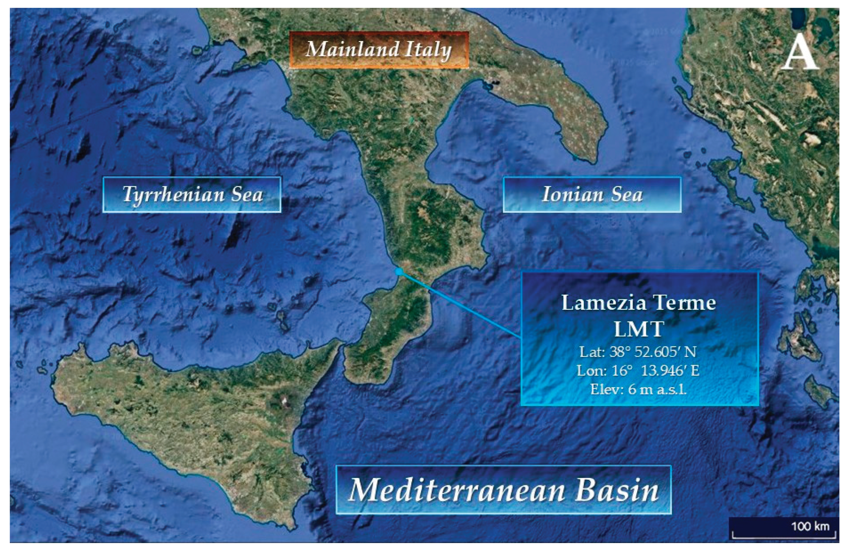
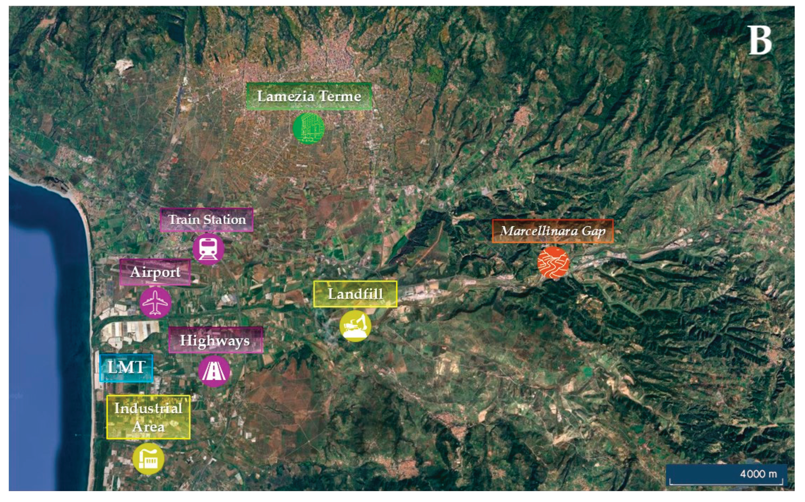
Figure 2.
Average concentrations of (A) CO (ppb), (A) CO2 (ppm), (A) CH4 (ppb), (D) SO2 (ppb), and (E) eBC (µg/m3) based on proximity categories and wind corridors (Continental: 0–90 °N; Seaside: 240–300 °N; Total: all directions).
Figure 2.
Average concentrations of (A) CO (ppb), (A) CO2 (ppm), (A) CH4 (ppb), (D) SO2 (ppb), and (E) eBC (µg/m3) based on proximity categories and wind corridors (Continental: 0–90 °N; Seaside: 240–300 °N; Total: all directions).
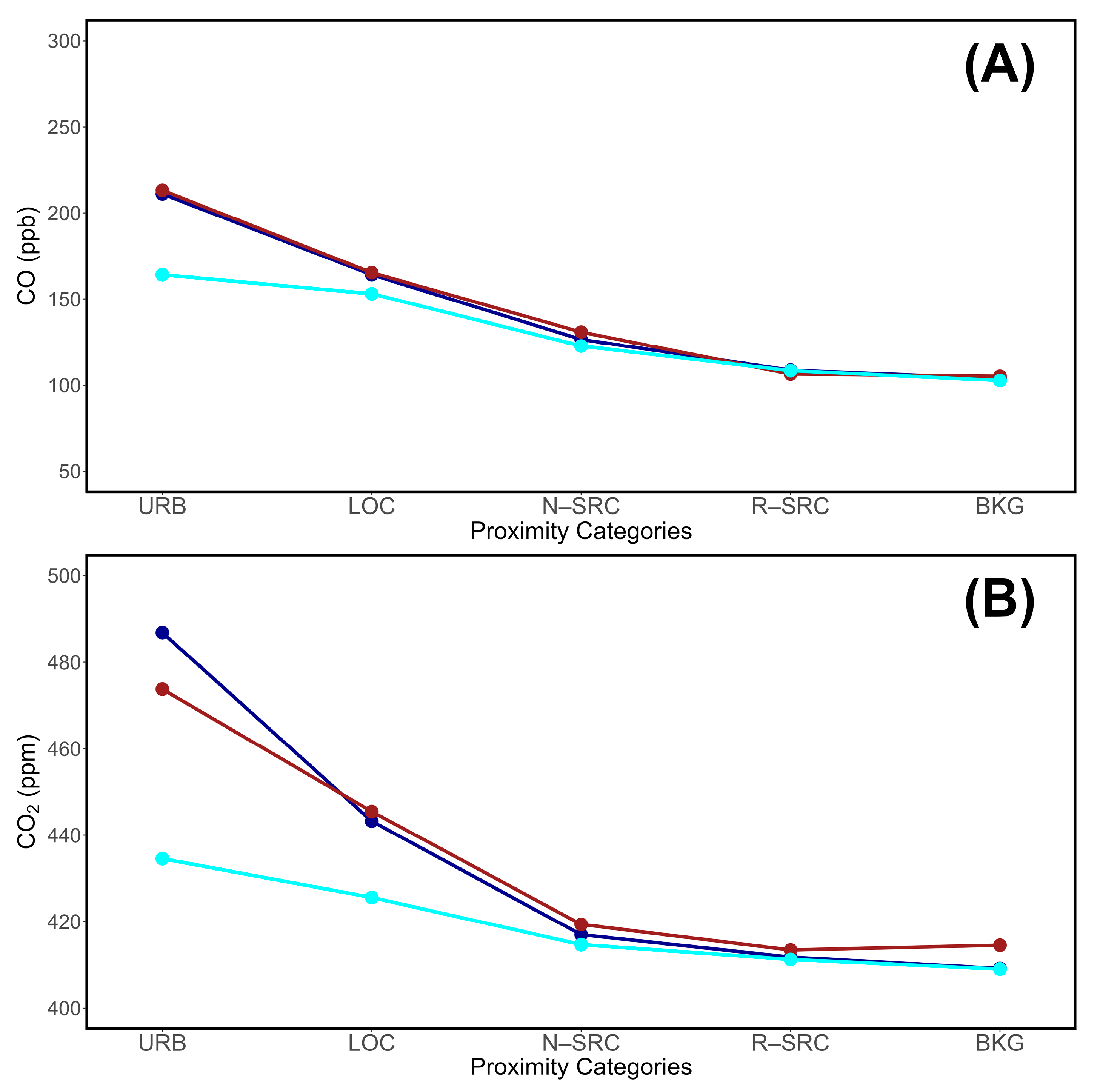
Figure 3.
Average concentrations of (A) CO (ppb), (A) CO2 (ppm), (A) CH4 (ppb), (D) SO2 (ppb), and (E) eBC (µg/m3) based on proximity categories and seasons.
Figure 3.
Average concentrations of (A) CO (ppb), (A) CO2 (ppm), (A) CH4 (ppb), (D) SO2 (ppb), and (E) eBC (µg/m3) based on proximity categories and seasons.
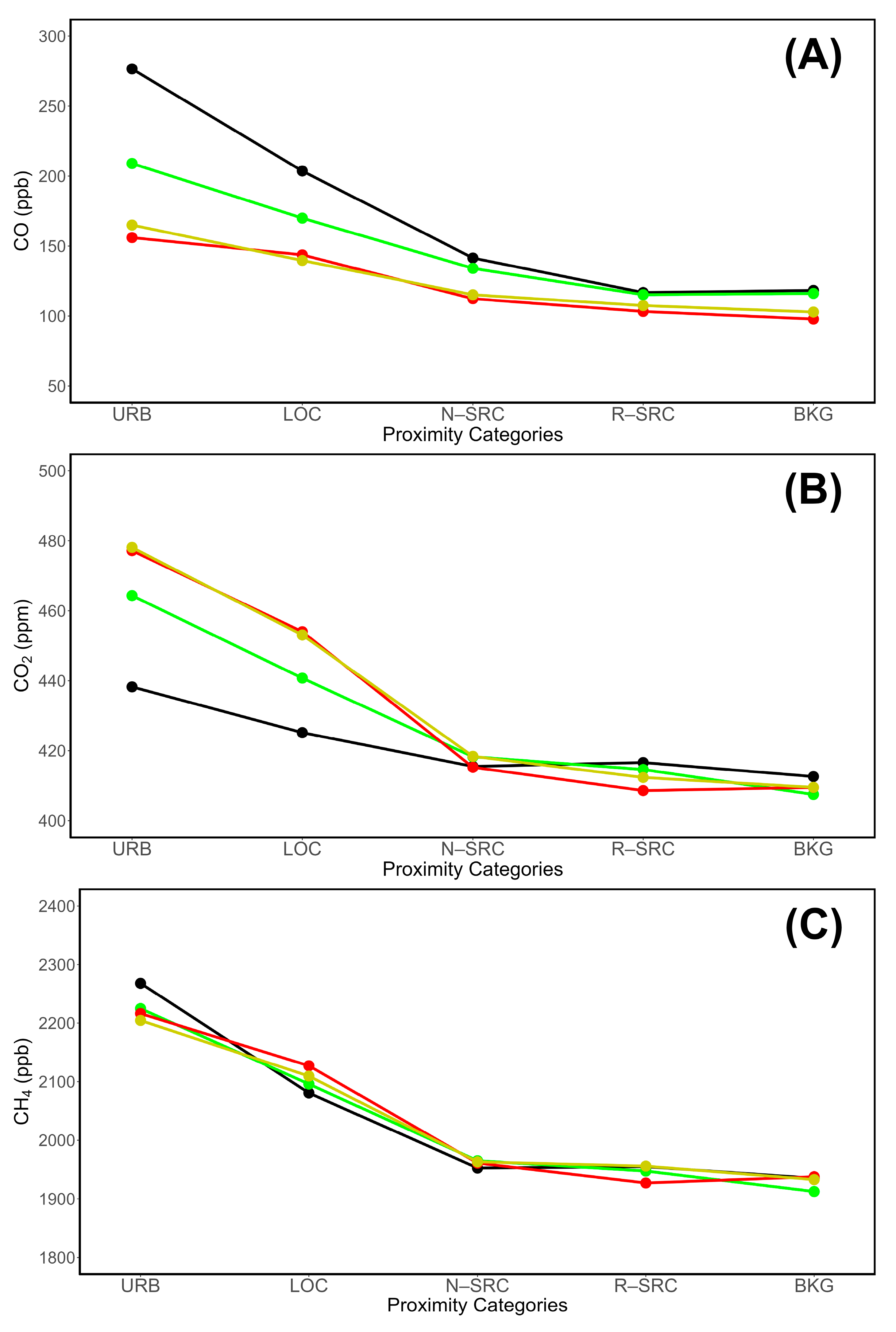
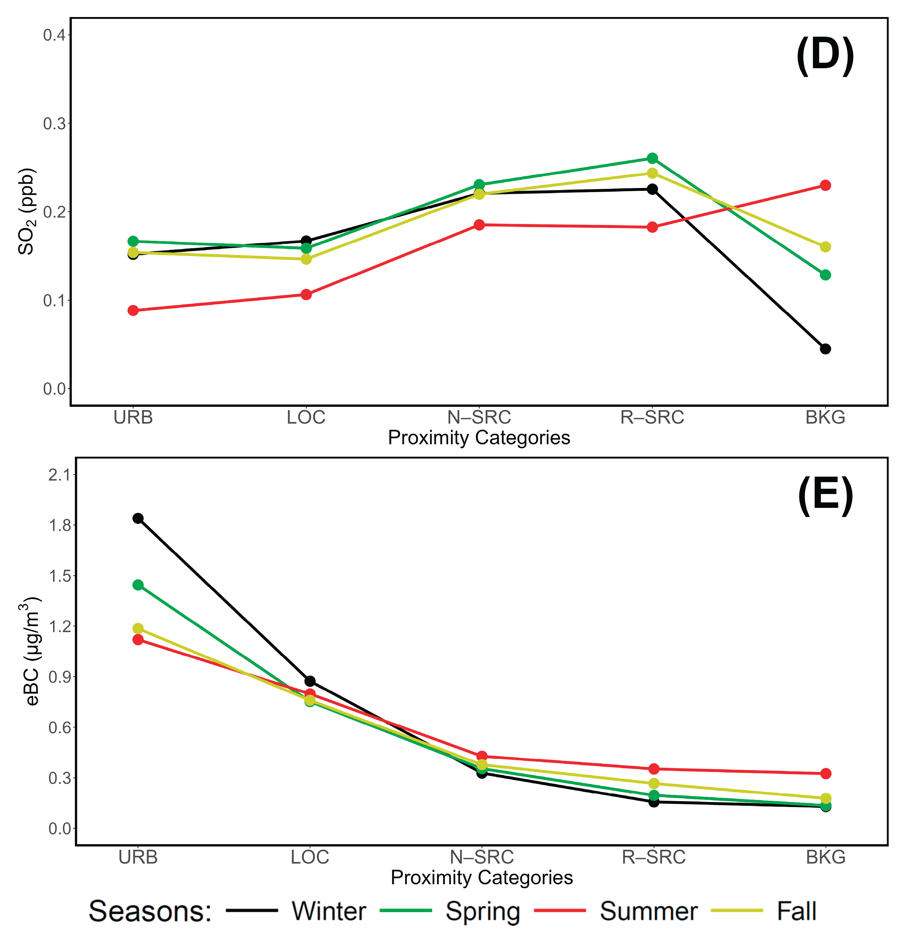
Figure 4.
Daily cycle variability of (A) CO (ppb), (A) CO2 (ppm), (A) CH4 (ppb), (D) SO2 (ppb), and (E) eBC (µg/m3) based on proximity categories.
Figure 4.
Daily cycle variability of (A) CO (ppb), (A) CO2 (ppm), (A) CH4 (ppb), (D) SO2 (ppb), and (E) eBC (µg/m3) based on proximity categories.
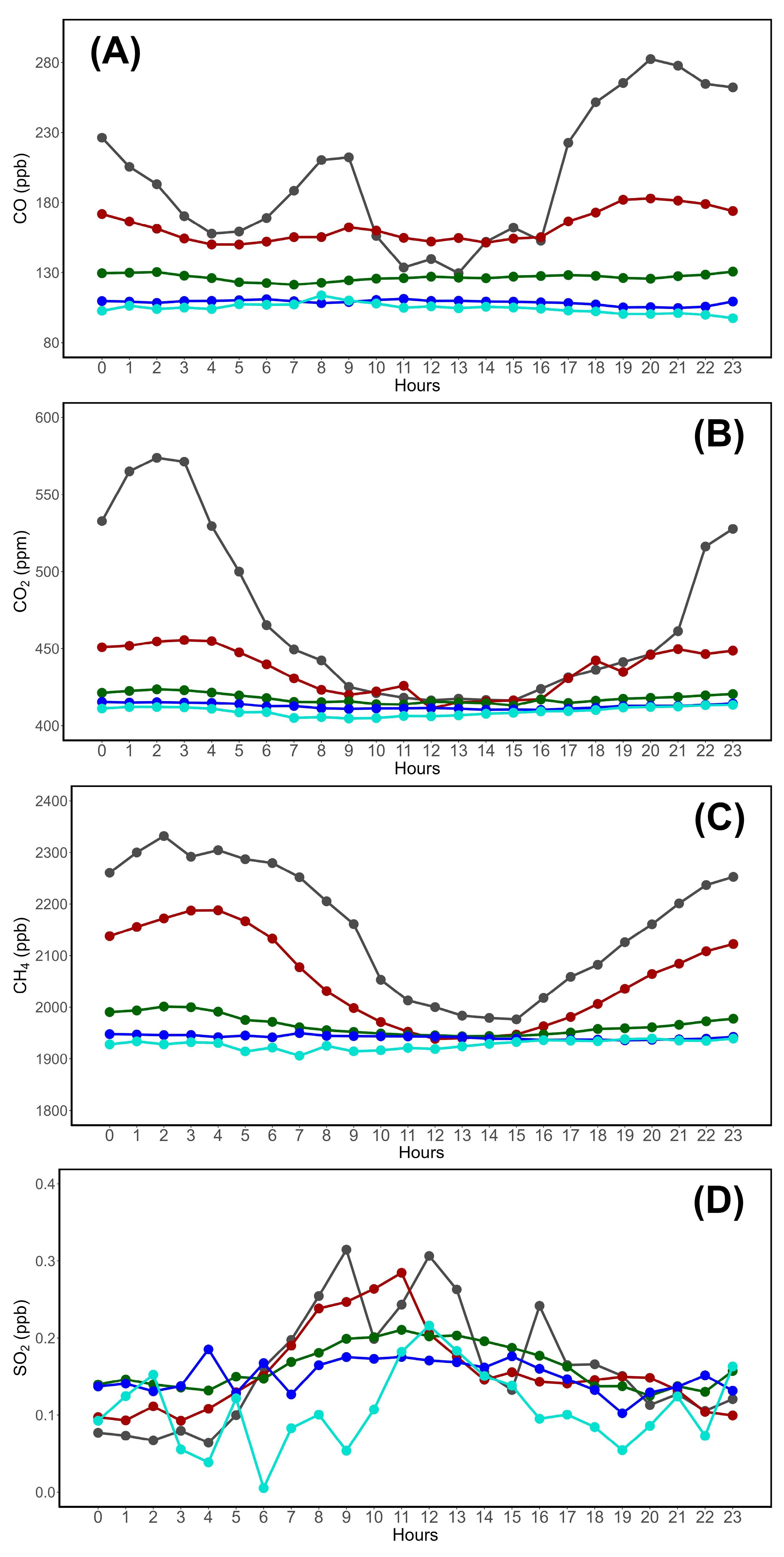
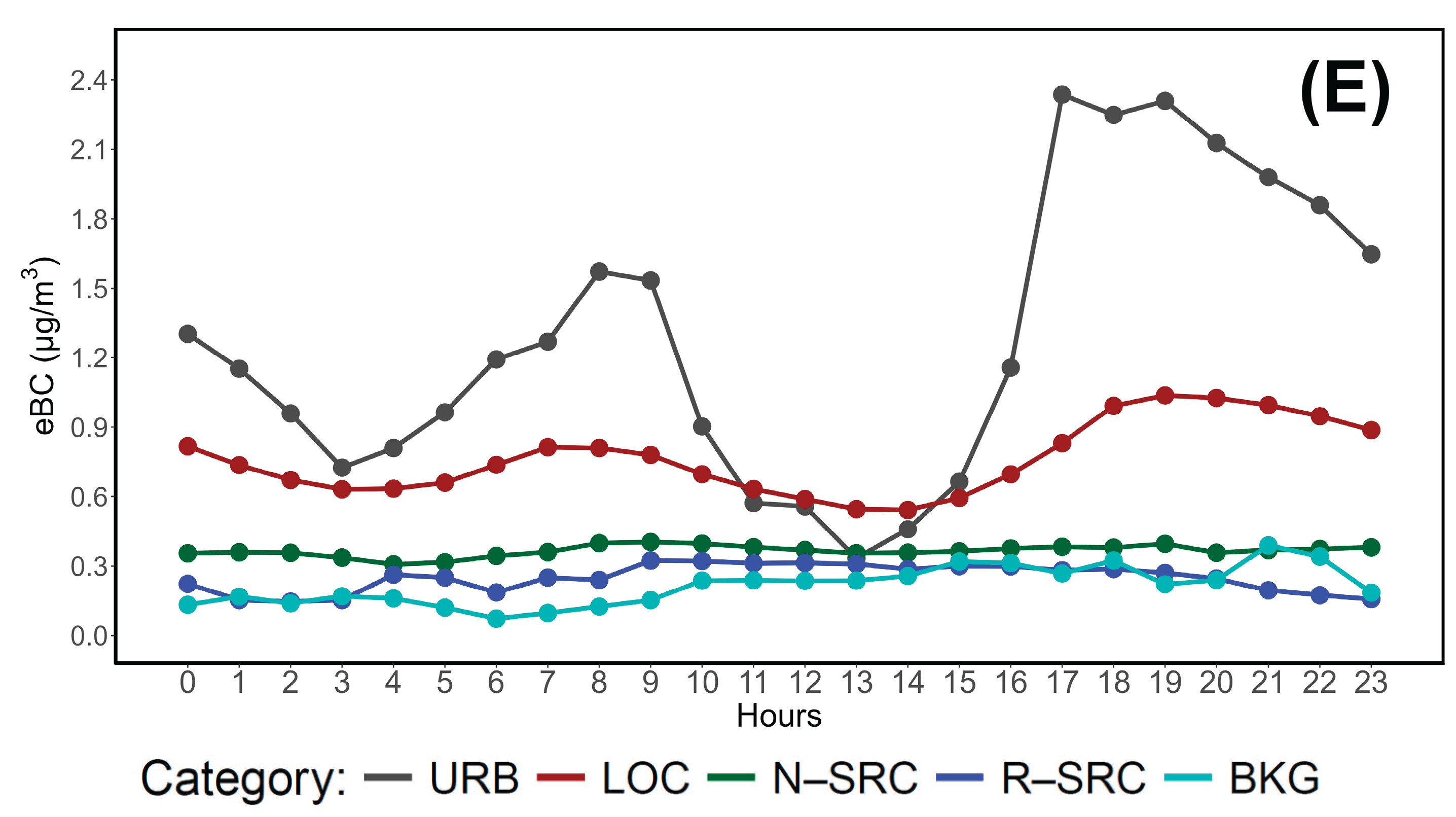
Figure 5.
Daily cycle variability, during the Winter season, of (A) CO (ppb), (A) CO2 (ppm), (A) CH4 (ppb), (D) SO2 (ppb), and (E) eBC (µg/m3) based on proximity categories.
Figure 5.
Daily cycle variability, during the Winter season, of (A) CO (ppb), (A) CO2 (ppm), (A) CH4 (ppb), (D) SO2 (ppb), and (E) eBC (µg/m3) based on proximity categories.
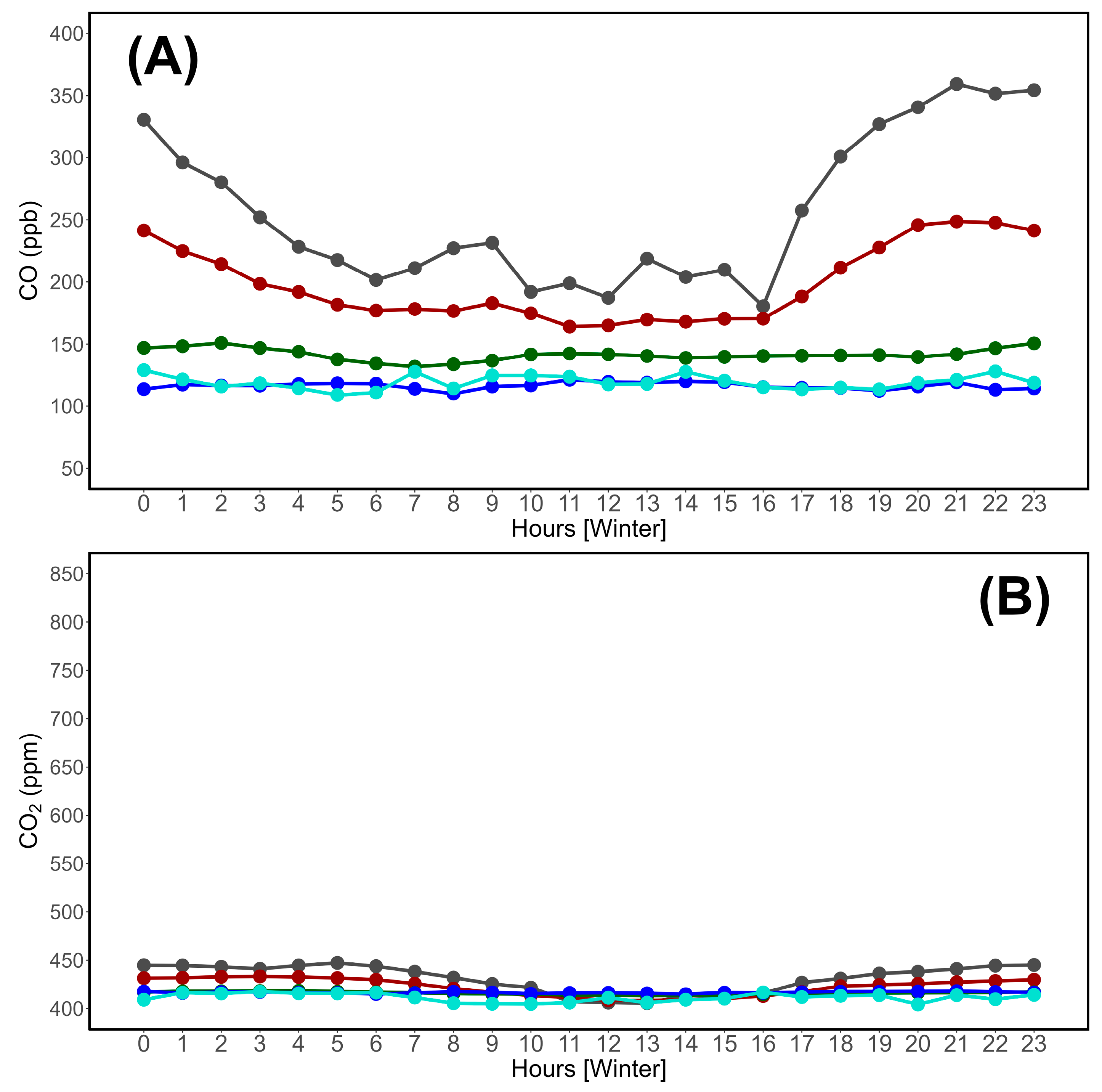
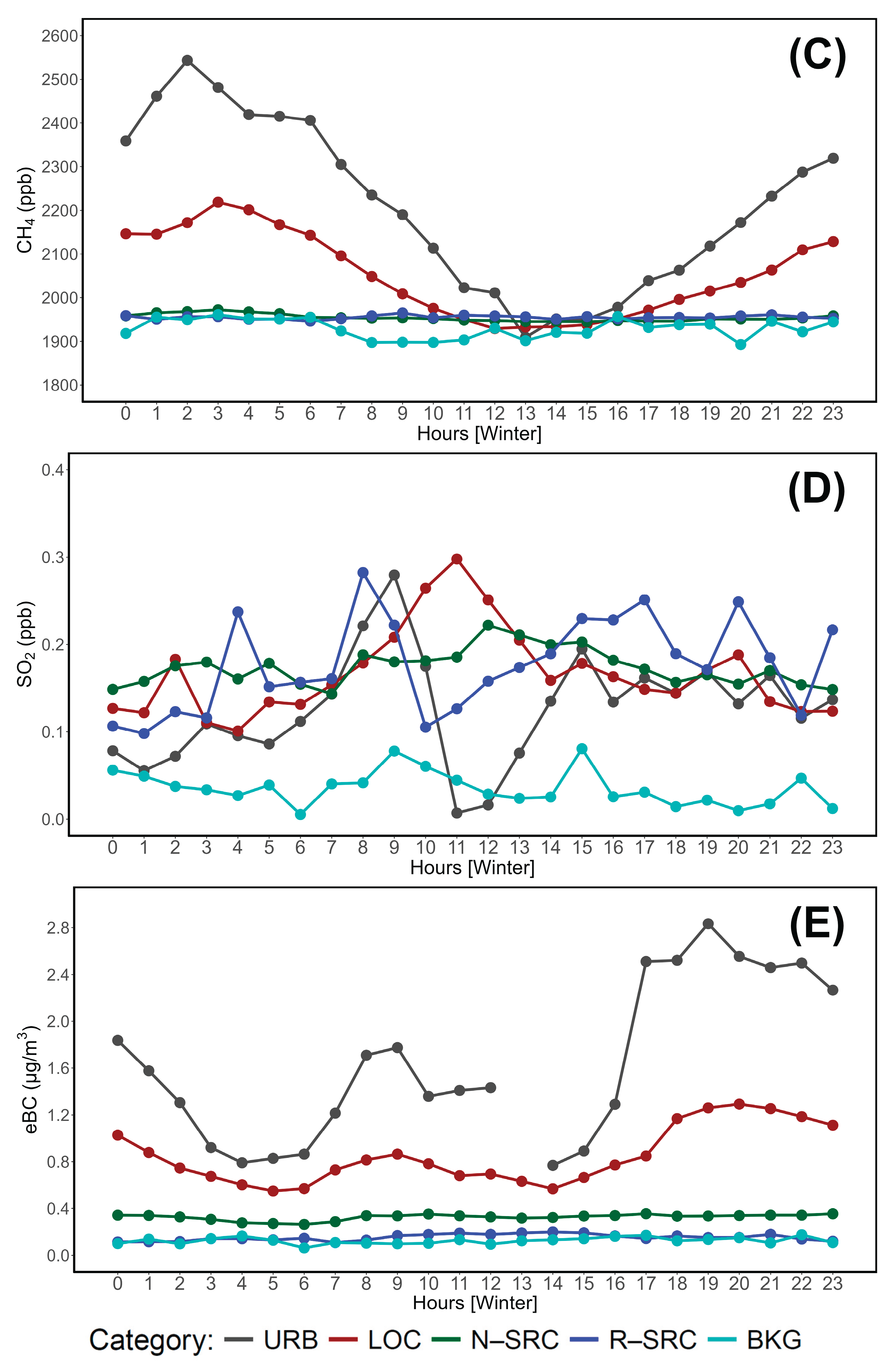
Figure 6.
Daily cycle variability, during the Spring season, of (A) CO (ppb), (A) CO2 (ppm), (A) CH4 (ppb), (D) SO2 (ppb), and (E) eBC (µg/m3) based on proximity categories.
Figure 6.
Daily cycle variability, during the Spring season, of (A) CO (ppb), (A) CO2 (ppm), (A) CH4 (ppb), (D) SO2 (ppb), and (E) eBC (µg/m3) based on proximity categories.
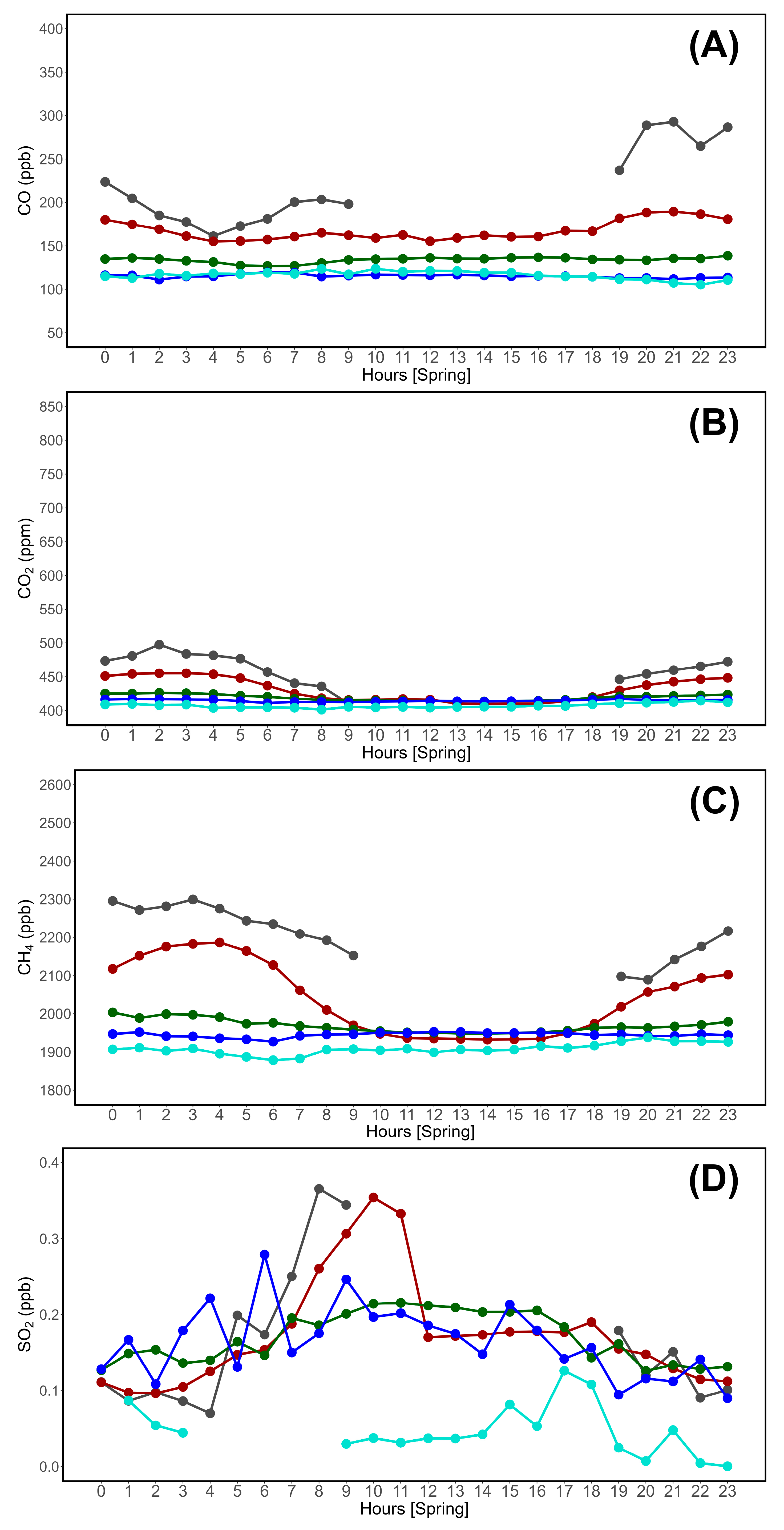
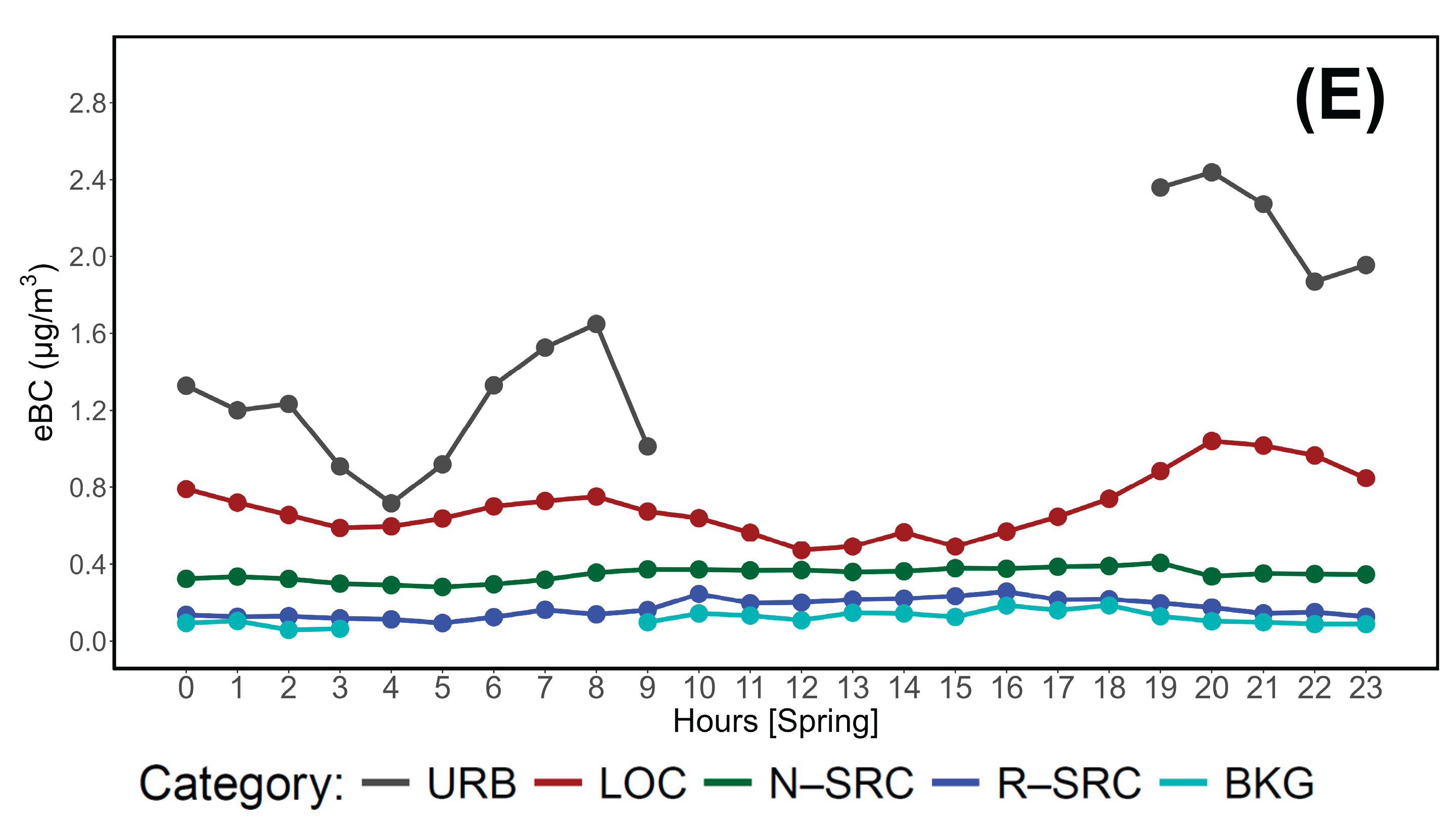
Figure 7.
Daily cycle variability, during the Summer season, of (A) CO (ppb), (A) CO2 (ppm), (A) CH4 (ppb), (D) SO2 (ppb), and (E) eBC (µg/m3) based on proximity categories.
Figure 7.
Daily cycle variability, during the Summer season, of (A) CO (ppb), (A) CO2 (ppm), (A) CH4 (ppb), (D) SO2 (ppb), and (E) eBC (µg/m3) based on proximity categories.
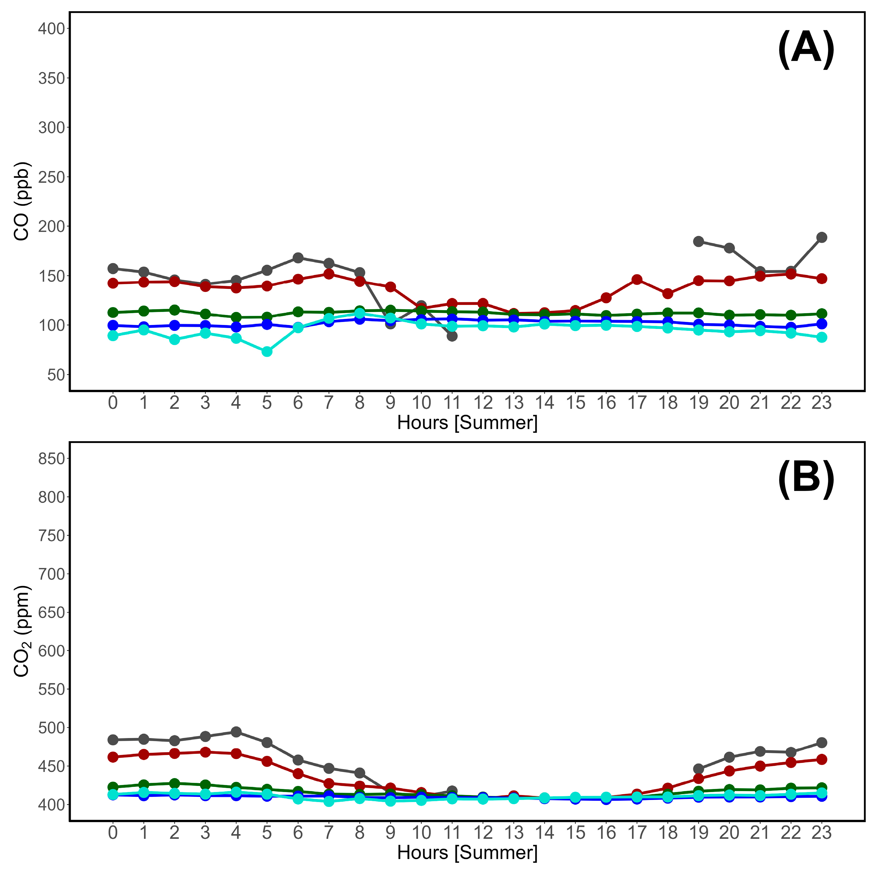
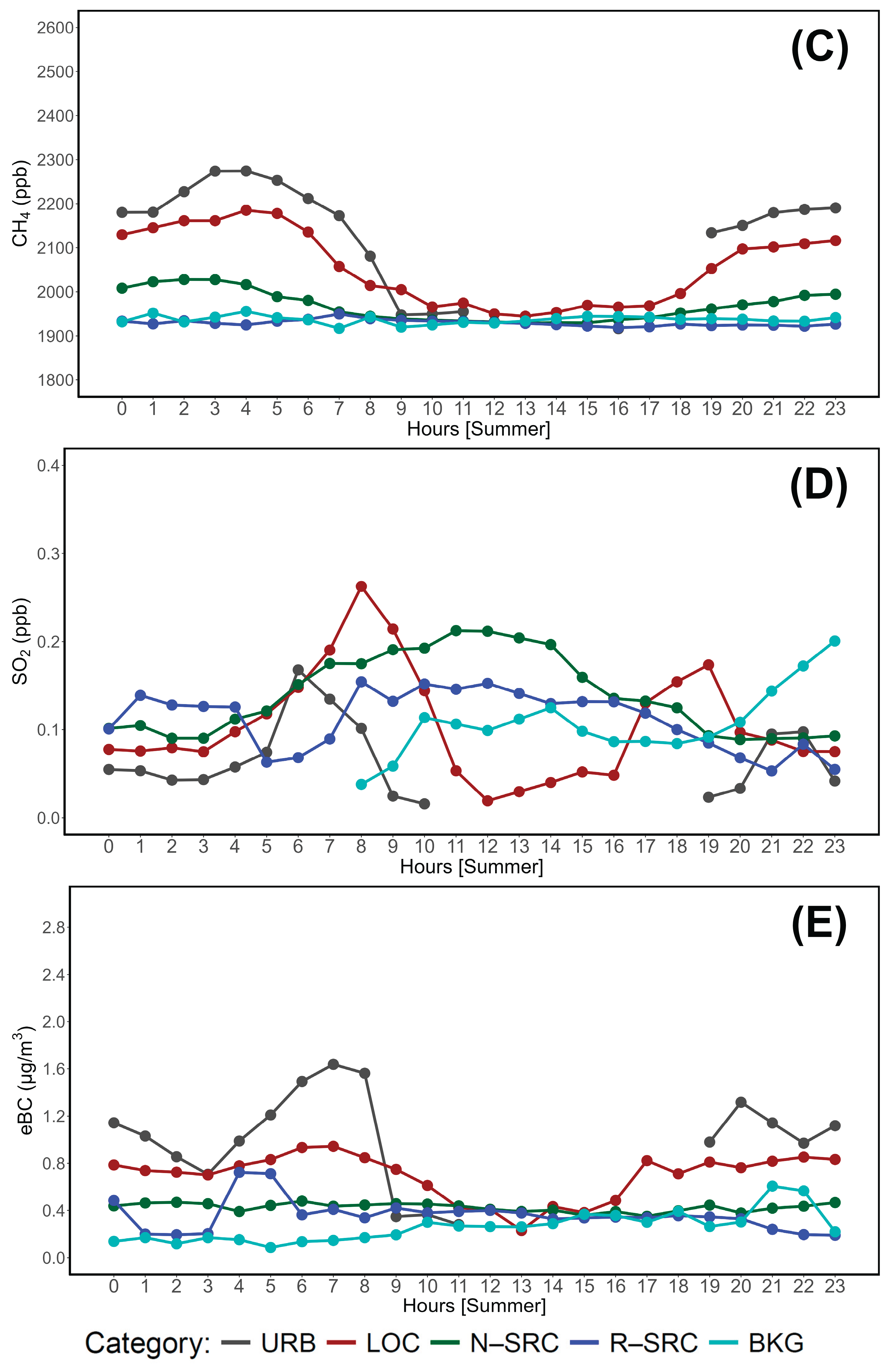
Figure 8.
Daily cycle variability, during the Fall season, of (A) CO (ppb), (A) CO2 (ppm), (A) CH4 (ppb), (D) SO2 (ppb), and (E) eBC (µg/m3) based on proximity categories.
Figure 8.
Daily cycle variability, during the Fall season, of (A) CO (ppb), (A) CO2 (ppm), (A) CH4 (ppb), (D) SO2 (ppb), and (E) eBC (µg/m3) based on proximity categories.
Figure 9.
Probability distribution of CO (ppb), CO2 (ppm), and CH4 (ppb) based on proximity category and wind direction. The radius of each polar plot refers to the concentration range of observed mole fractions.
Figure 9.
Probability distribution of CO (ppb), CO2 (ppm), and CH4 (ppb) based on proximity category and wind direction. The radius of each polar plot refers to the concentration range of observed mole fractions.
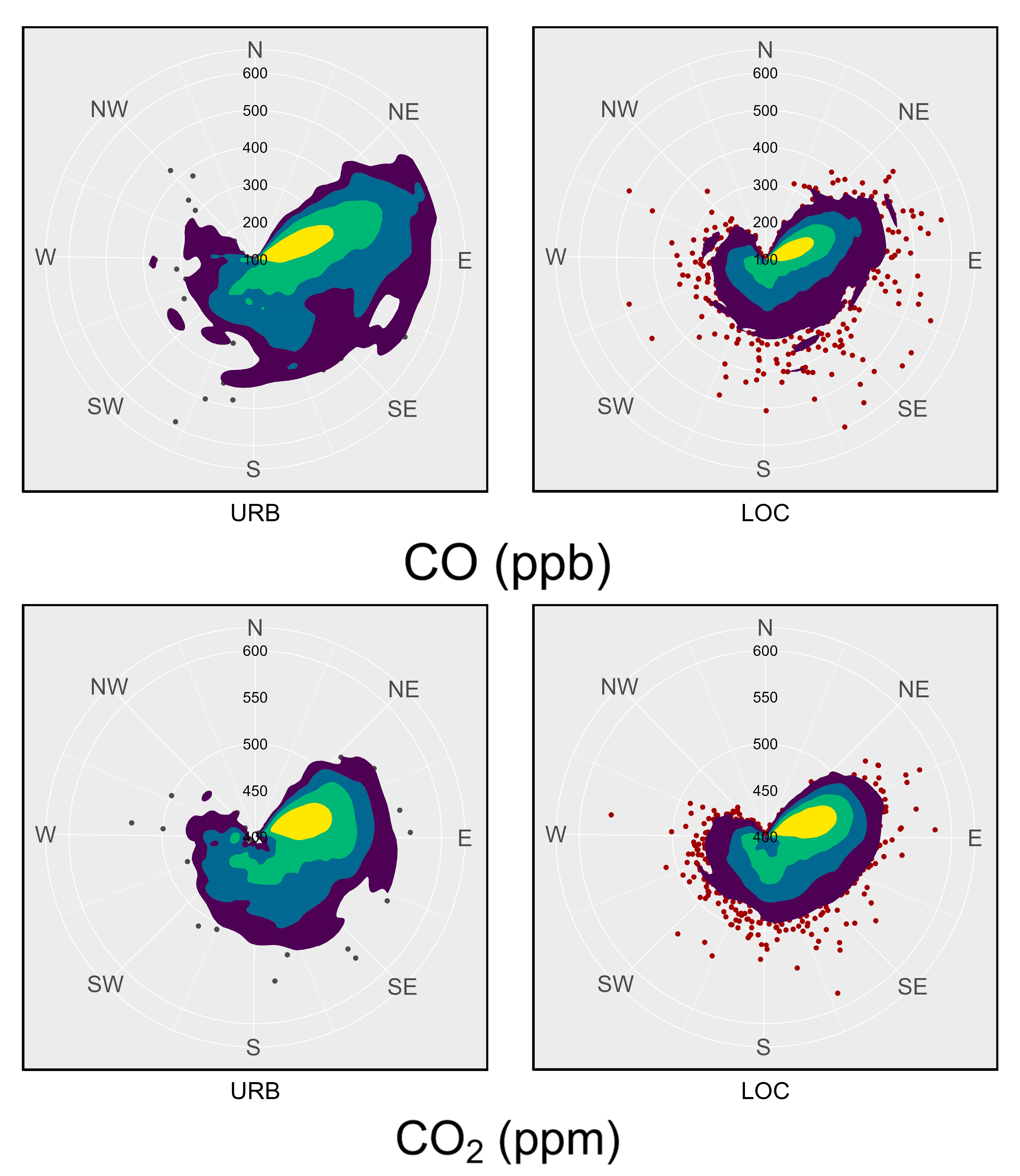
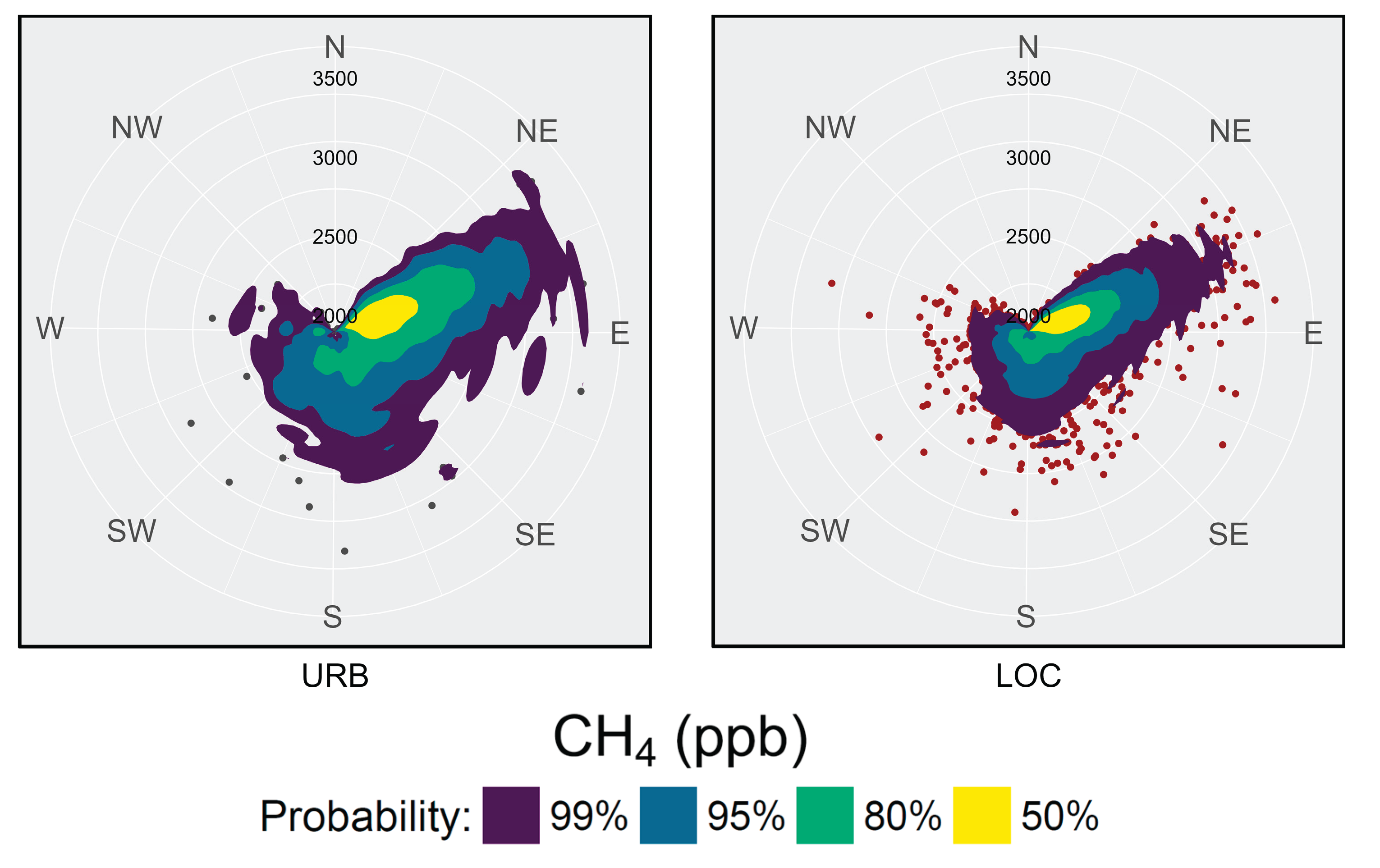
Figure 10.
Probability distribution of SO2 (ppb) and eBC (µg/m3) based on proximity category and wind direction. The radius of each polar plot refers to the concentration range of observed concentrations.
Figure 10.
Probability distribution of SO2 (ppb) and eBC (µg/m3) based on proximity category and wind direction. The radius of each polar plot refers to the concentration range of observed concentrations.
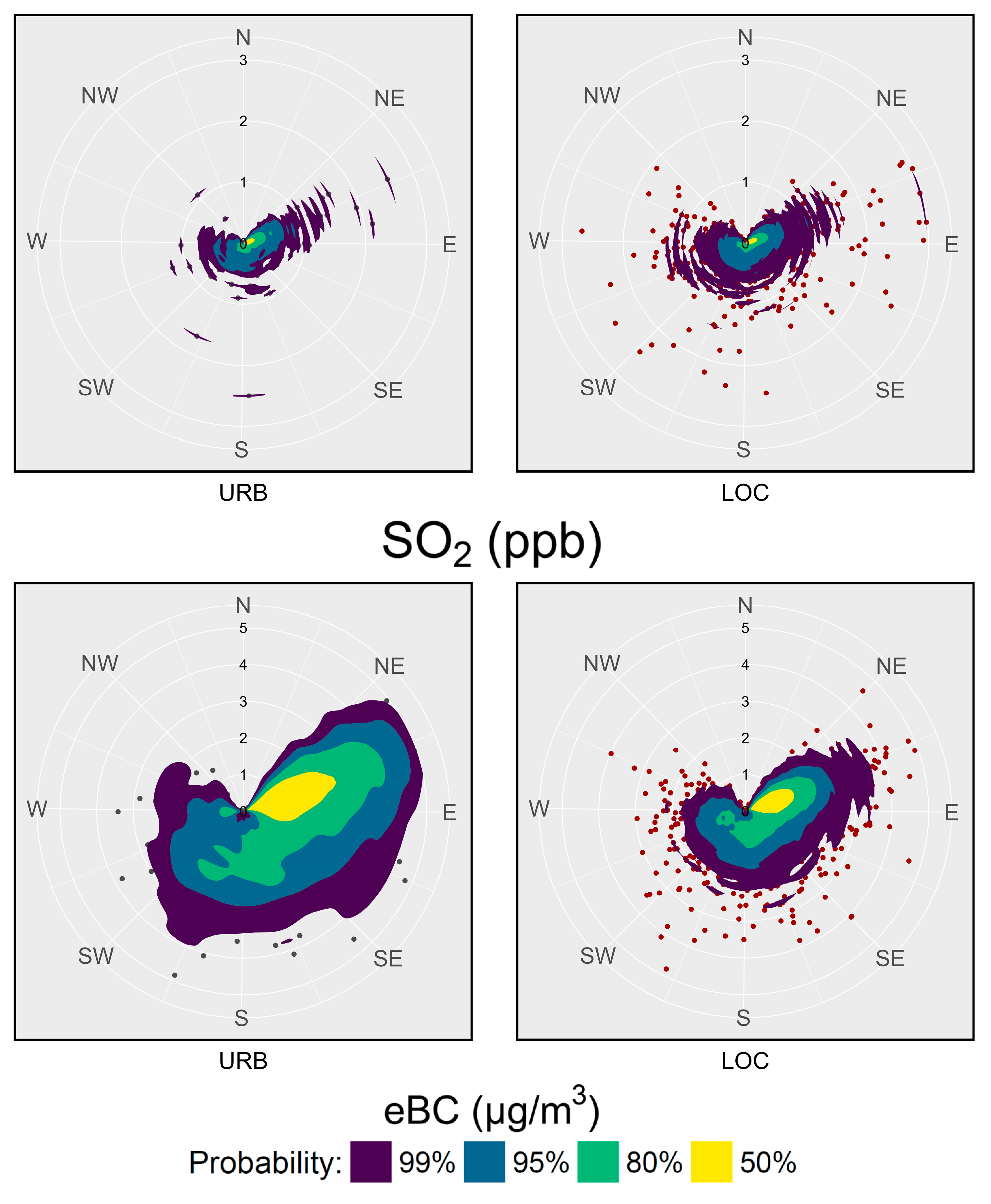
Figure 11.
Density distribution plots showing the probability distribution of wind speed (m/s) and (A) CO (ppb), (B) CO2 (ppm), (C) CH4 (ppb), (D) SO2 (ppb), and (E) eBC (μg/m3), for URB (left) and LOC (right) proximity categories. These plots refer to all wind directions.
Figure 11.
Density distribution plots showing the probability distribution of wind speed (m/s) and (A) CO (ppb), (B) CO2 (ppm), (C) CH4 (ppb), (D) SO2 (ppb), and (E) eBC (μg/m3), for URB (left) and LOC (right) proximity categories. These plots refer to all wind directions.
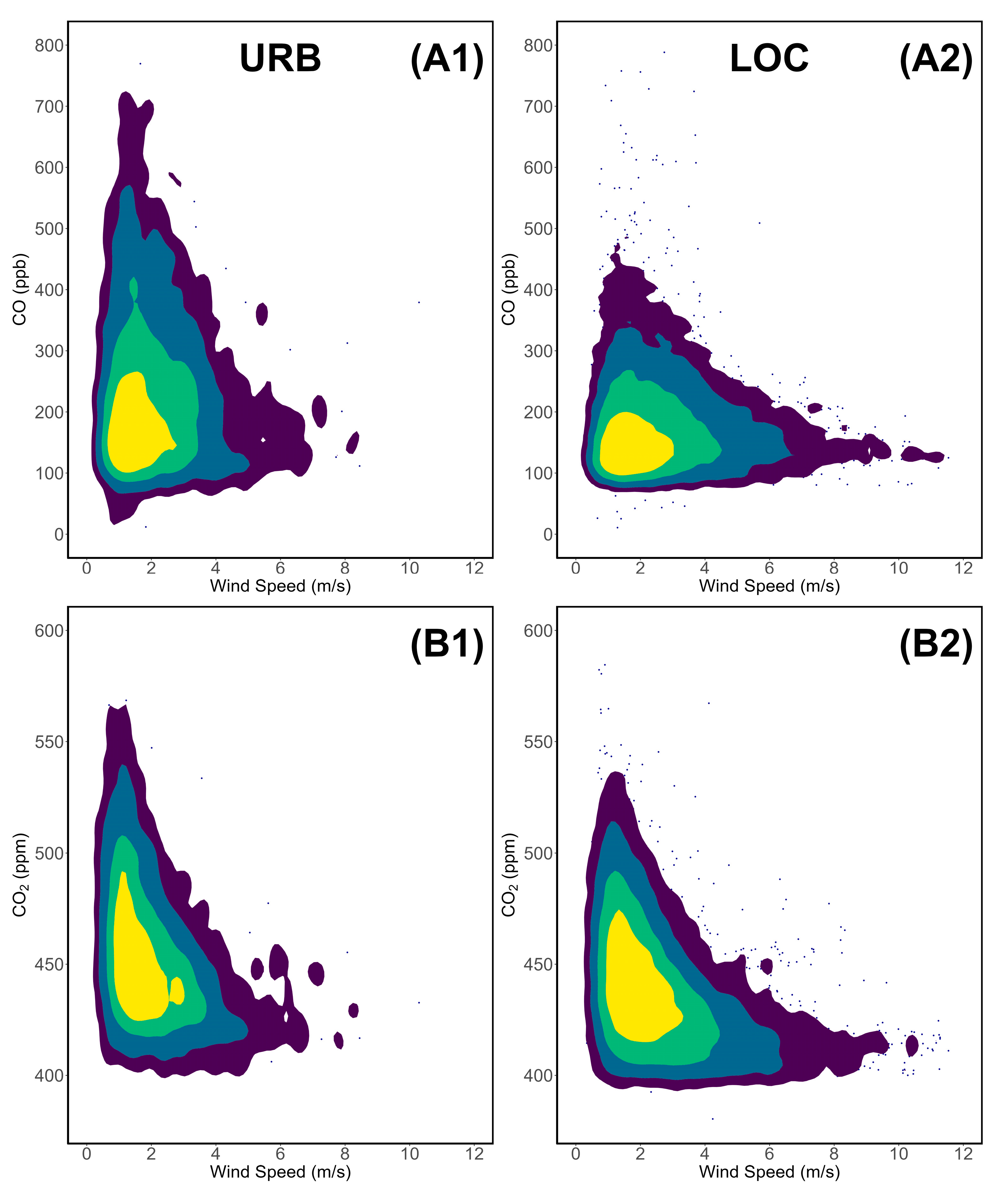
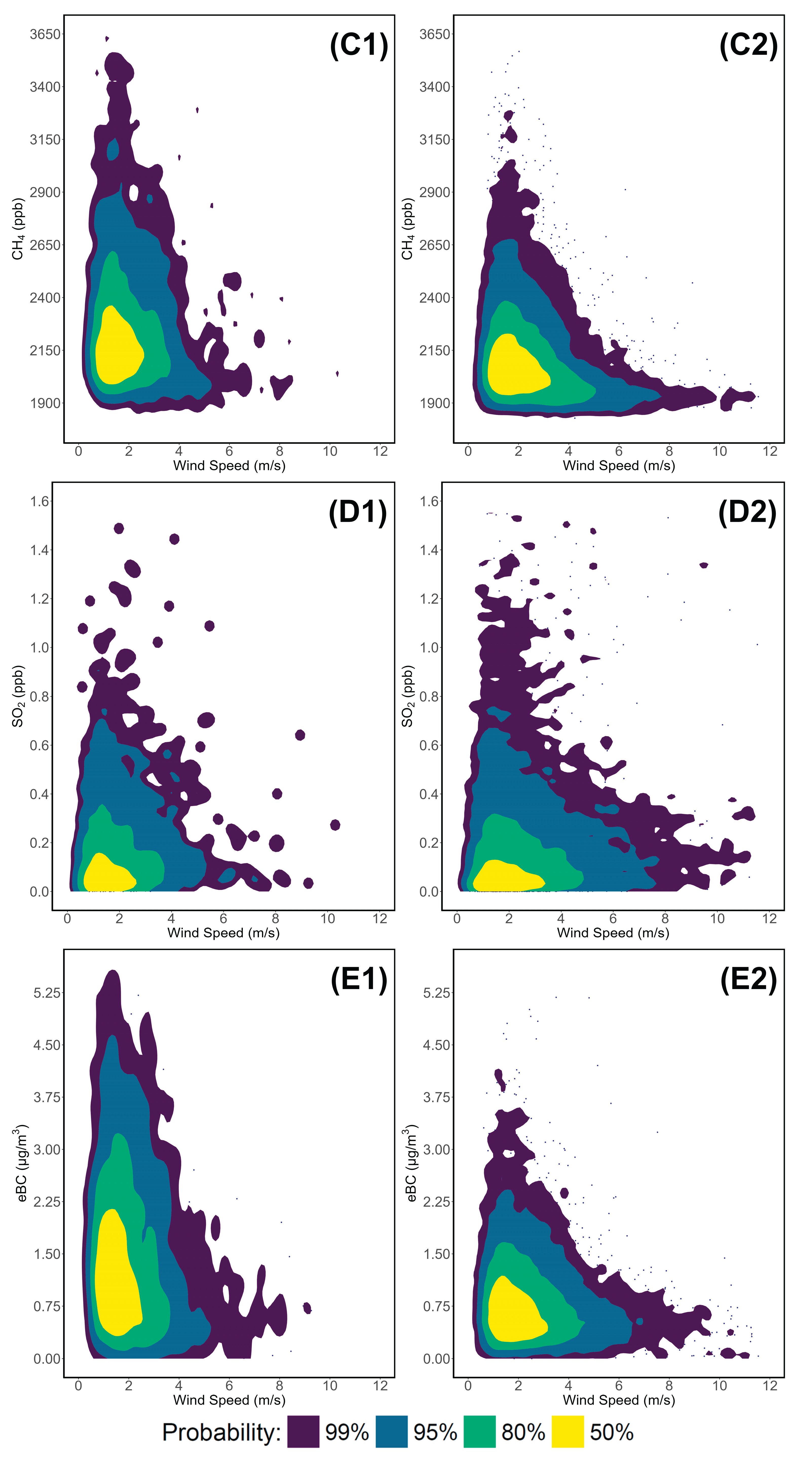
Figure 12.
Density distribution plots showing the probability distribution of wind speed (m/s) and (A) CO (ppb), (B) CO2 (ppm), (C) CH4 (ppb), (D) SO2 (ppb), and (E) eBC (μg/m3), for URB (left) and LOC (right) proximity categories. These plots refer to the western-seaside wind corridor (240–300 °N from LMT).

Figure 13.
Density distribution plots showing the probability distribution of wind speed (m/s) and (A) CO (ppb), (B) CO2 (ppm), (C) CH4 (ppb), (D) SO2 (ppb), and (E) eBC (μg/m3), for URB (left) and LOC (right) proximity categories. These plots refer to the northeastern-continental wind corridor (0–90 °N from LMT).
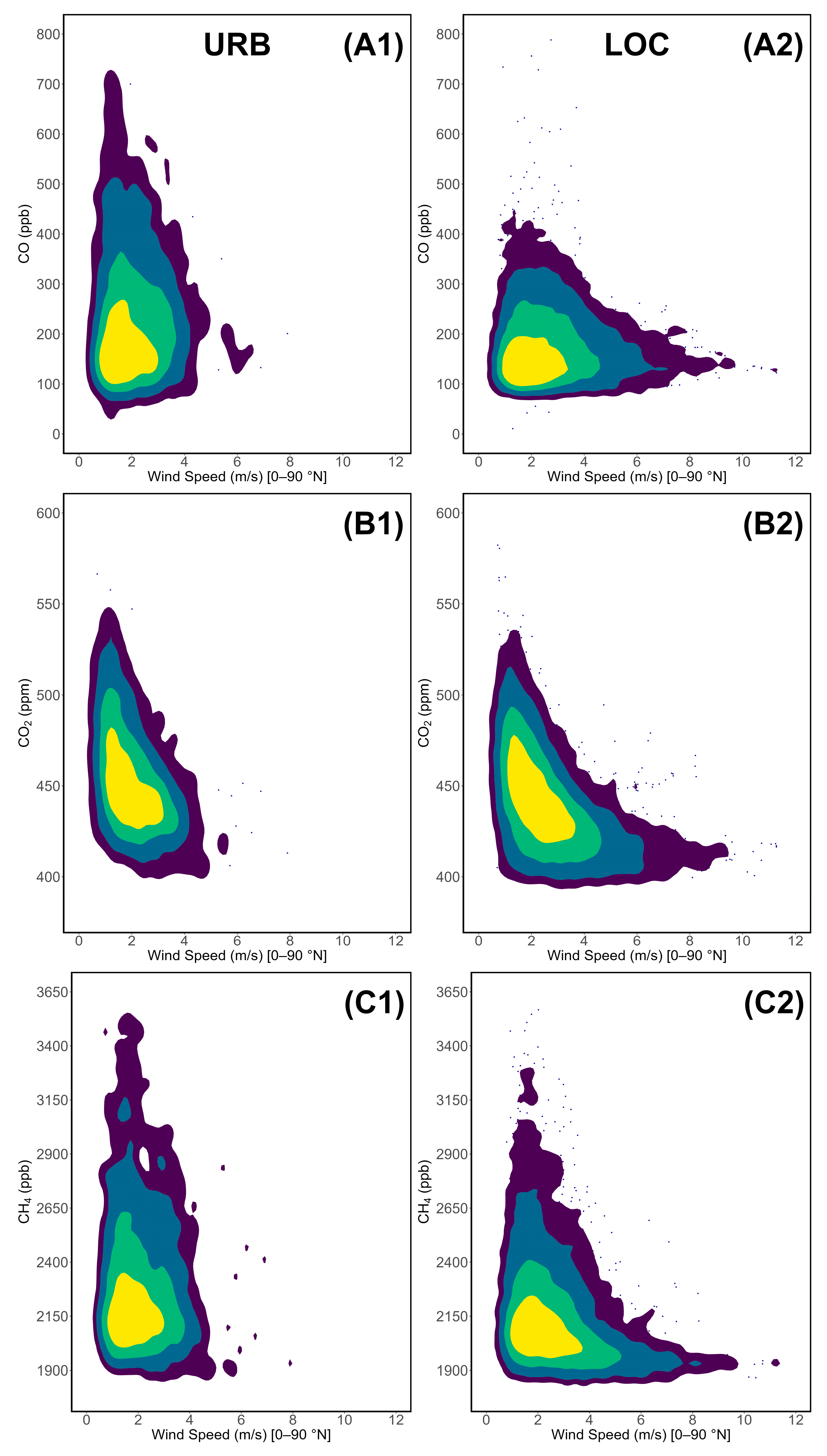

Figure 14.
Weekly cycle of (A) CO (ppb), (B) CO2 (ppm), (C) CH4 (ppb), (D) SO2 (ppb), and (E) eBC (μg/m3) accounting for all wind directions at LMT.
Figure 14.
Weekly cycle of (A) CO (ppb), (B) CO2 (ppm), (C) CH4 (ppb), (D) SO2 (ppb), and (E) eBC (μg/m3) accounting for all wind directions at LMT.
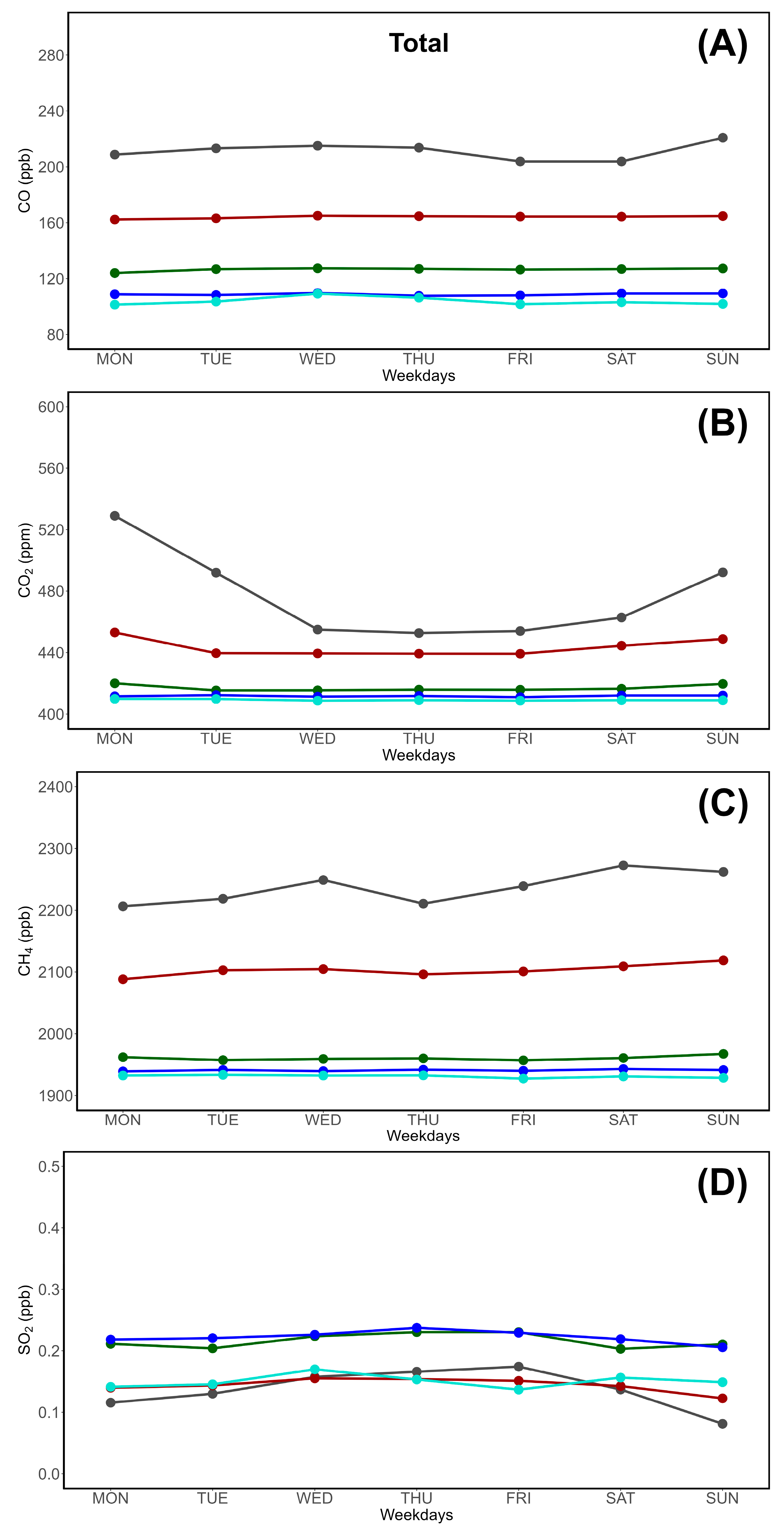
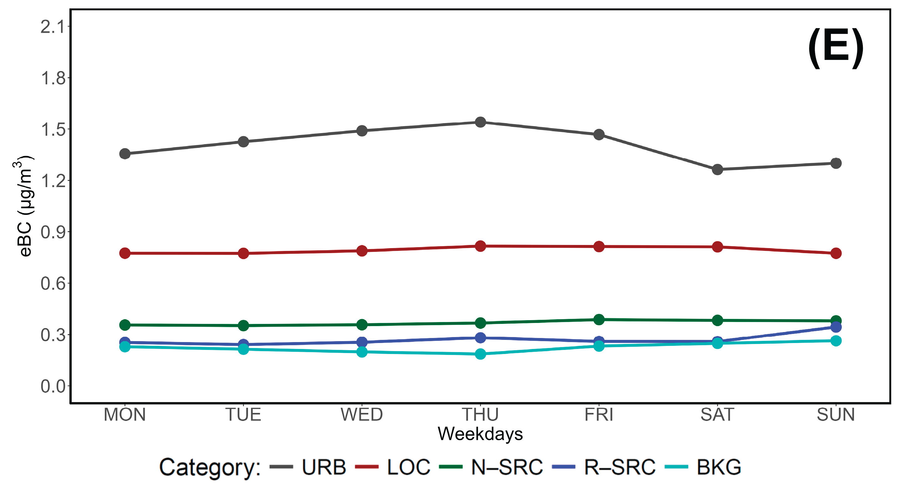
Figure 15.
Weekly cycle of (A) CO (ppb), (B) CO2 (ppm), (C) CH4 (ppb), (D) SO2 (ppb), and (E) eBC (μg/m3) accounting for the western-seaside wind corridor (240–300 °N).
Figure 15.
Weekly cycle of (A) CO (ppb), (B) CO2 (ppm), (C) CH4 (ppb), (D) SO2 (ppb), and (E) eBC (μg/m3) accounting for the western-seaside wind corridor (240–300 °N).
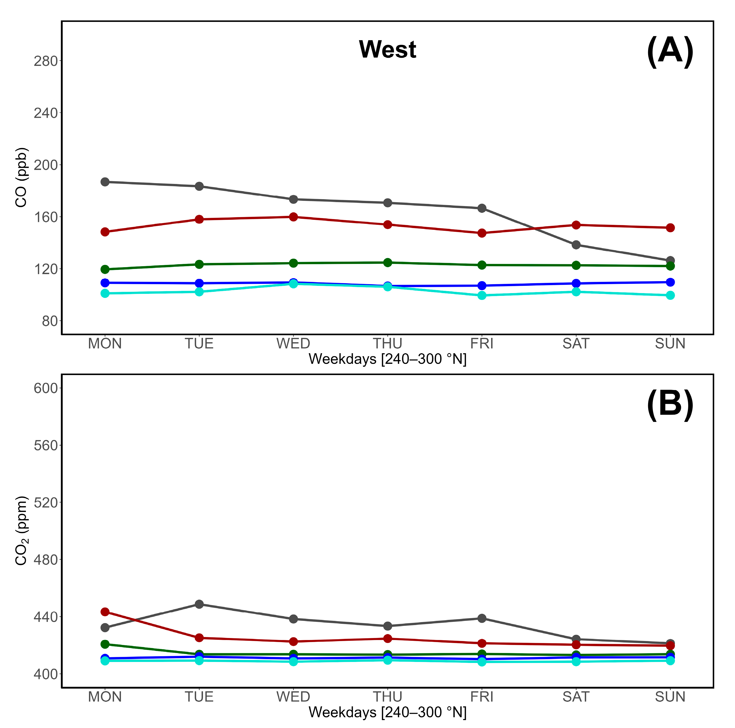
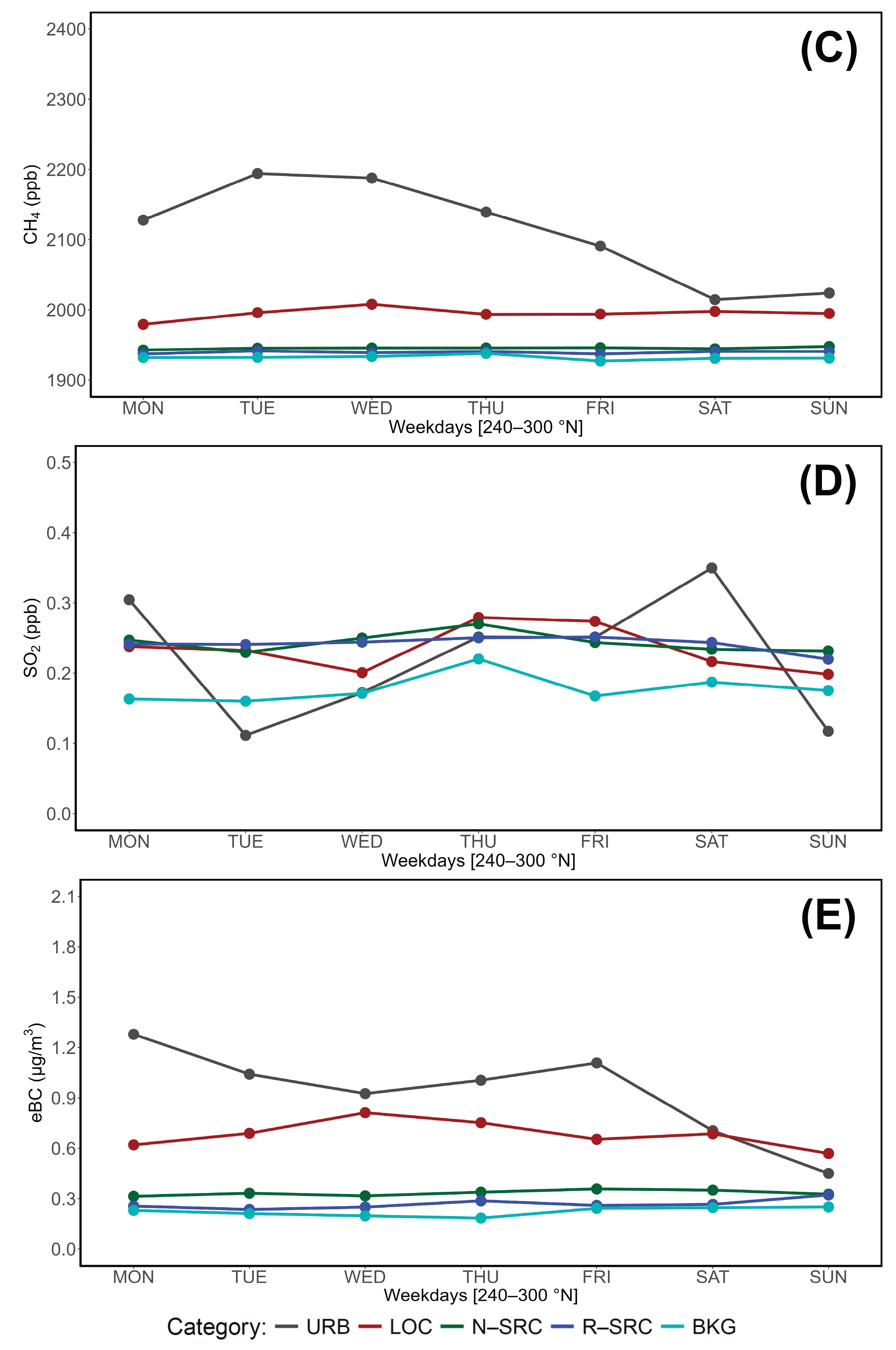
Figure 16.
Weekly cycle of (A) CO (ppb), (B) CO2 (ppm), (C) CH4 (ppb), (D) SO2 (ppb), and (E) eBC (μg/m3) accounting for the northeastern-continental wind corridor (0–90 °N).
Figure 16.
Weekly cycle of (A) CO (ppb), (B) CO2 (ppm), (C) CH4 (ppb), (D) SO2 (ppb), and (E) eBC (μg/m3) accounting for the northeastern-continental wind corridor (0–90 °N).
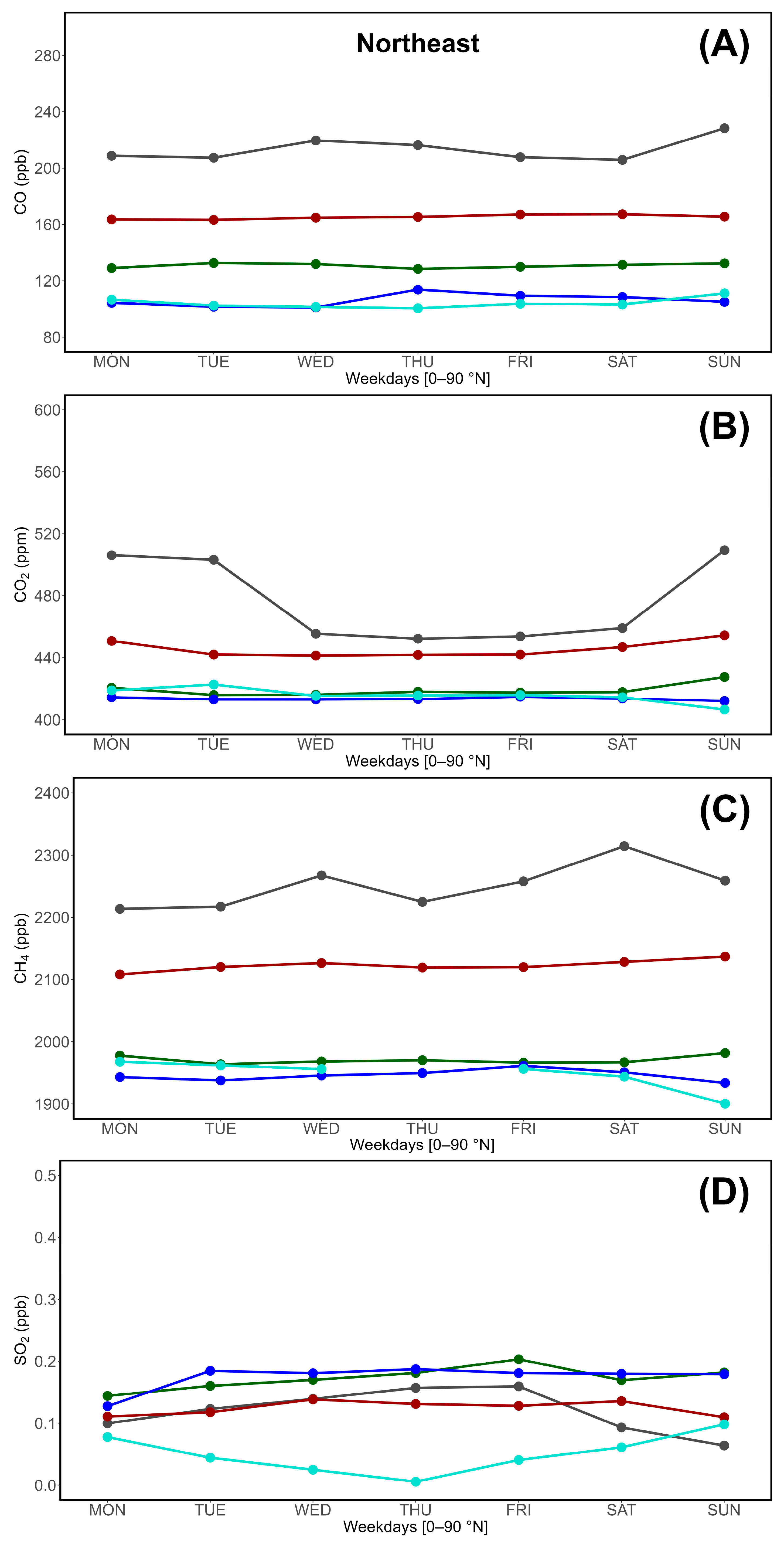
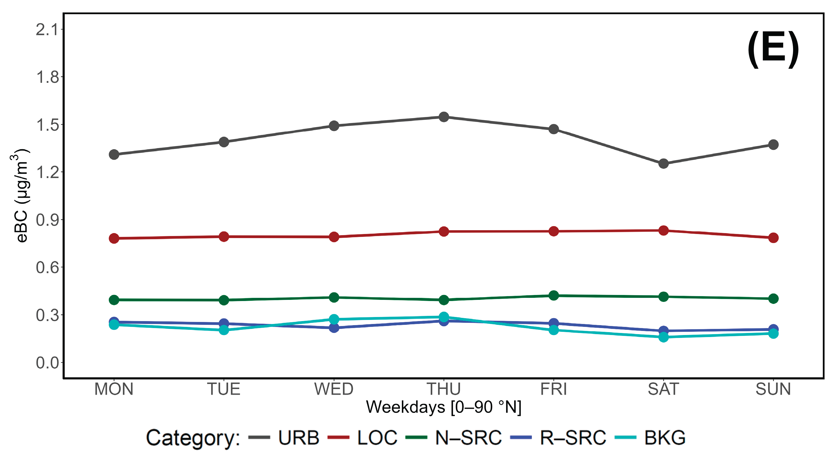
Figure 17.
Multi-year tendencies of (A) CO (ppb), (B) CO2 (ppm), (C) CH4 (ppb), (D) SO2 (ppb), and (E) eBC (μg/m3) based on proximity categories and monthly averaged data.
Figure 17.
Multi-year tendencies of (A) CO (ppb), (B) CO2 (ppm), (C) CH4 (ppb), (D) SO2 (ppb), and (E) eBC (μg/m3) based on proximity categories and monthly averaged data.
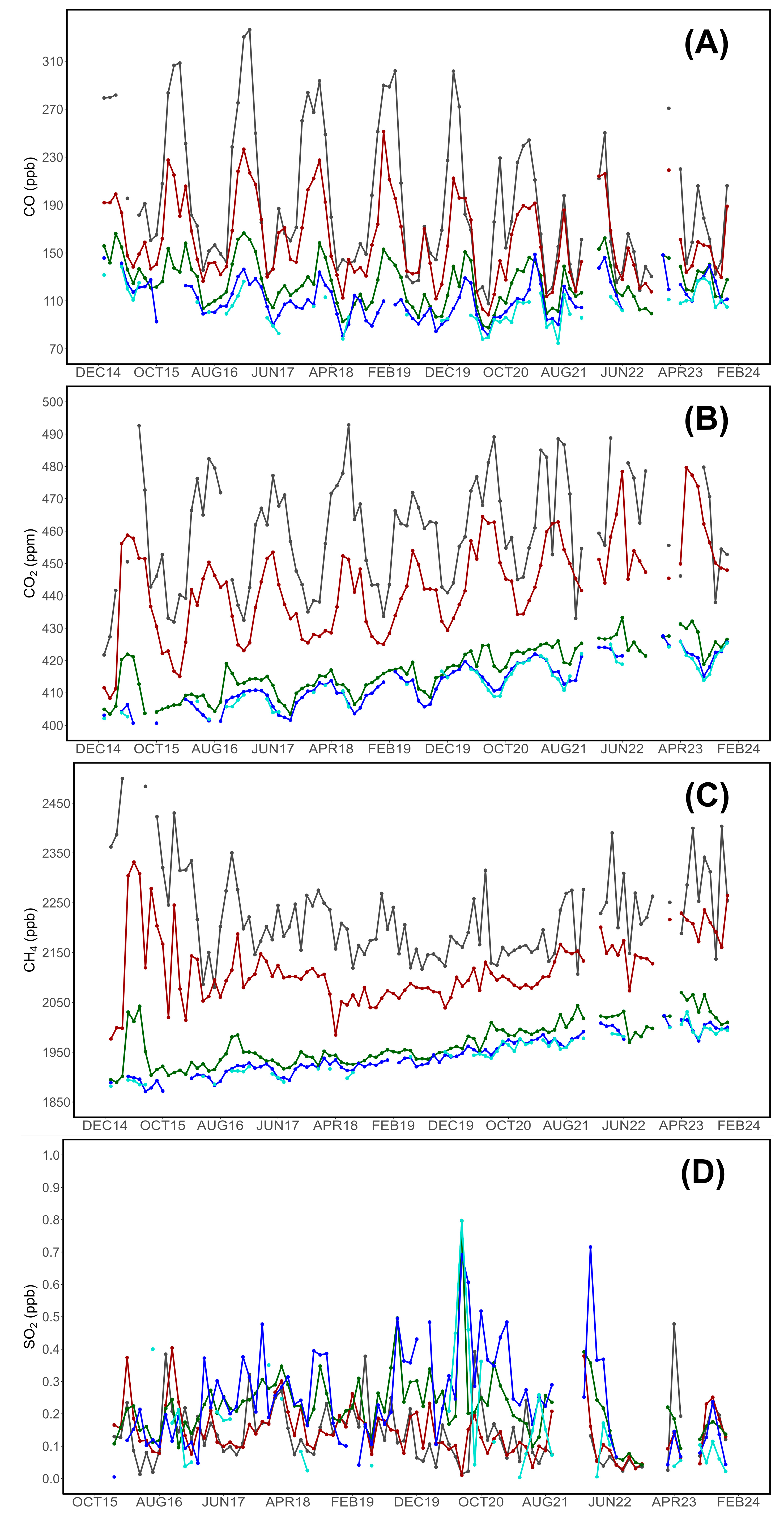
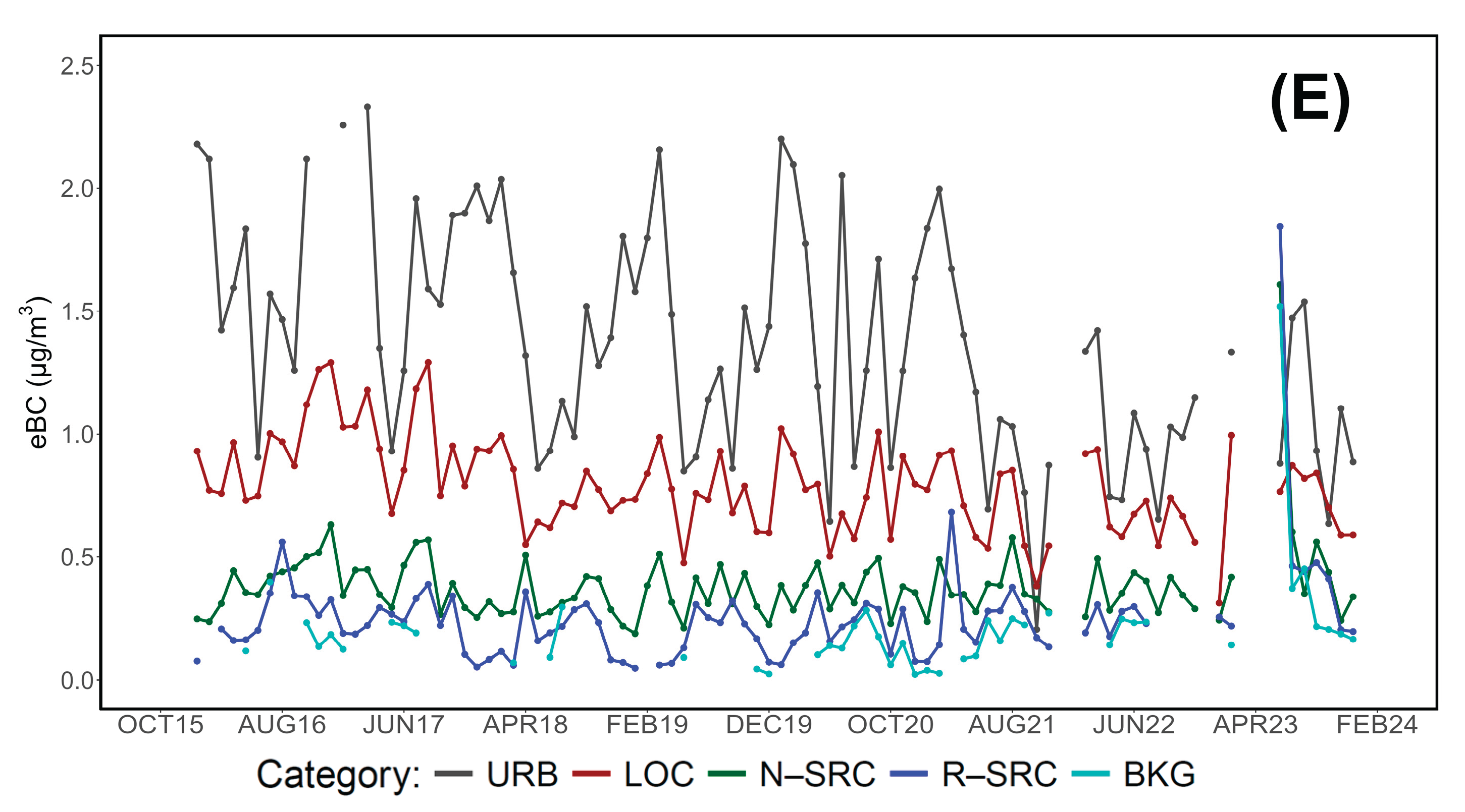

Table 1.
Distribution of URB and LOC hourly data coverage during the entire observation period (2015-2023). Previous research studies at LMT allocated URB hours under the LOC category.
Table 1.
Distribution of URB and LOC hourly data coverage during the entire observation period (2015-2023). Previous research studies at LMT allocated URB hours under the LOC category.
| Year | Hours | URB | LOC |
|---|---|---|---|
| 2015 | 8760 | 5.7% | 39.33% |
| 2016 | 8784 | 3.32% | 25.63% |
| 2017 | 8760 | 4.70% | 30.35% |
| 2018 | 8760 | 6.64% | 35.30% |
| 2019 | 8760 | 5.97% | 33.59% |
| 2020 | 8784 | 4.42% | 30.80% |
| 2021 | 8760 | 2.57% | 24.80% |
| 2022 | 8760 | 4.31% | 26.56% |
| 2023 | 8760 | 3.66% | 23.59% |
| Total | 701281 | 4.59%2 | 30.01%2 |
1 Sum of all hours. 1 Average rate.
Table 2.
Coverage rates of the hourly COx (CO + CO2) and CH4 datasets used in this study. The CMTO dataset combines Picarro G2401 (CO, CO2, CH4) and Vaisala WXT520 (meteorological parameters) measurements. CProx combines Picarro G2401 measurements with hourly data for which a proximity category could be defined, i.e. valid Thermo Scientific 49i (O3) and Thermo Scientific 42i-TL (NOx) data. CMTOProx combines all previous datasets, thus resulting in lower coverage rates throughout the 2015-2023 period.
| Year | Hours | COx, CH4 | Meteo | CMTO | CProx | CMTOProx |
|---|---|---|---|---|---|---|
| 2015 | 8760 | 94.73% | 95.90% | 92.10% | 87.85% | 86.97% |
| 2016 | 8784 | 94.95% | 96.34% | 92.24% | 89.89% | 88.21% |
| 2017 | 8760 | 99.57% | 93.8% | 93.37% | 95.27% | 90.67% |
| 2018 | 8760 | 93.78% | 77.05% | 74.68% | 92.11% | 73.34% |
| 2019 | 8760 | 97.60% | 98.59% | 97.57% | 93.28% | 93.26% |
| 2020 | 8784 | 93.77% | 99.98% | 93.76% | 89.10% | 89.09% |
| 2021 | 8760 | 97.78% | 99.74% | 97.53% | 77.35% | 77.34% |
| 2022 | 8760 | 83.89% | 89.85% | 75.46% | 59.15% | 58.04% |
| 2023 | 8760 | 66.76% | 96.3% | 65.49% | 58.44% | 57.18% |
| Total | 701281 | 91.43%2 | 93.95%2 | 86.91%2 | 82.49%2 | 79.34%2 |
1 Sum of all hours. 2 Average rate.
Table 3.
Coverage rates of the hourly SO2 datasets used in this study. The SMTO dataset combines Thermo Scientific 32i (SO2) and Vaisala WXT520 (meteorological parameters) measurements. SProx combines Thermo Scientific 32i measurements with hourly data for which a proximity category could be defined, i.e. valid Thermo Scientific 49i (O3) and Thermo Scientific 42i-TL (NOx) data. SMTOProx combines all previous datasets, thus resulting in lower coverage rates throughout the 2016-2023 period.
| Year | Hours | SO2 | Meteo | SMTO | SProx | SMTOProx |
|---|---|---|---|---|---|---|
| 2016 | 8784 | 63.30% | 96.34% | 62.04% | 61.28% | 60.04% |
| 2017 | 8760 | 87.76% | 93.8% | 83.86% | 86.11% | 82.23% |
| 2018 | 8760 | 97.54% | 77.05% | 75.18% | 97.04% | 74.69% |
| 2019 | 8760 | 80.67% | 98.59% | 80.65% | 77.65% | 77.63% |
| 2020 | 8784 | 34.52% | 99.98% | 34.52% | 33.03% | 33.03% |
| 2021 | 8760 | 39.08% | 99.74% | 39.07% | 35.45% | 35.44% |
| 2022 | 8760 | 65.06% | 89.85% | 63.75% | 62.48% | 61.44% |
| 2023 | 8760 | 48.59% | 96.3% | 47.37% | 48.07% | 46.86% |
| Total | 701281 | 64.56%2 | 93.95%2 | 60.80%2 | 62.63%2 | 58.92%2 |
1 Sum of all hours. 2 Average rate.
Table 4.
Coverage rates of the hourly eBC datasets used in this study. The BMTO dataset combines Thermo Scientific 5012 (eBC) and Vaisala WXT520 (meteorological parameters) measurements. BProx combines Thermo Scientific 5012 measurements with hourly data for which a proximity category could be defined, i.e. valid Thermo Scientific 49i (O3) and Thermo Scientific 42i-TL (NOx) data. BMTOProx combines all previous datasets, thus resulting in lower coverage rates throughout the 2016-2023 period.
| Year | Hours | eBC | Meteo | BMTO | BProx | BMTOProx |
|---|---|---|---|---|---|---|
| 2016 | 8784 | 93.75% | 96.34% | 93.06% | 89.70% | 89.20% |
| 2017 | 8760 | 95.27% | 93.8% | 90.45% | 92.24% | 87.93% |
| 2018 | 8760 | 95.61% | 77.05% | 73.61% | 94.44% | 72.5% |
| 2019 | 8760 | 96.48% | 98.59% | 96.46% | 92.26% | 92.23% |
| 2020 | 8784 | 96.61% | 99.98% | 96.60% | 91.75% | 91.74% |
| 2021 | 8760 | 98.42% | 99.74% | 98.25% | 77.39% | 77.38% |
| 2022 | 8760 | 97.43% | 89.85% | 88% | 67.37% | 65.98% |
| 2023 | 8760 | 69.13% | 96.3% | 68.81% | 60.51% | 60.19% |
| Total | 701281 | 92.83%2 | 93.95%2 | 88.15%2 | 83.20%2 | 79.64%2 |
1 Sum of all hours. 2 Average rate.
Table 5.
Concentrations of CO (ppb), CO2 (ppm), and CH4 (ppb) on a per-category basis, also including the ±1σ interval (one standard deviation). Data are divided by wind sector (Northeast = 0–90 °N; West = 240–300 °N).
Table 5.
Concentrations of CO (ppb), CO2 (ppm), and CH4 (ppb) on a per-category basis, also including the ±1σ interval (one standard deviation). Data are divided by wind sector (Northeast = 0–90 °N; West = 240–300 °N).
| Category | CO (ppb) | CO2 (ppm) | CH4 (ppb) | ||||||
| All | Nor. East | West | All | Nor. East | West | All | Nor. East | West | |
| URB | 212.85 ± 98.80 |
216.04 ± 100.66 |
164.10 ± 61.20 |
487.72 ± 516.99 |
474.28 ± 351.07 |
434.56 ± 19.71 |
2234.73 ± 231.80 |
2249.76 ± 237.06 |
2104.03 ± 155.84 |
| LOC | 164.69 ± 59.98 |
166.32 ± 60.50 |
153.03 ± 52.11 |
443.20 ± 123.73 |
445.54 ± 107.30 |
425.61 ± 139.46 |
2104.10 ± 175.34 |
2125.98 ± 186.55 |
1994.59 ± 112.39 |
| N–SRC | 127.13 ± 29.17 |
134.07 ± 31.86 |
122.73 ± 25.50 |
417.19 ± 54.21 |
420.53 ± 57.38 |
414.67 ± 65.35 |
1961.64 ± 67.87 |
1976.75 ± 81.63 |
1945.38 ± 39.59 |
| R–SRC | 109.45 ± 19.15 |
116.30 ± 15.12 |
108.43 ± 18.72 |
411.86 ± 8.60 |
416.20 ± 9.47 |
411.26 ± 8.45 |
1941.55 ± 43.14 |
1963.69 ± 44.13 |
1939.52 ± 41.45 |
| BKG | 104.04 ± 21.07 |
109.13 ± 11.09 |
102.75 ± 21.45 |
409.13 ± 7.83 |
415.60 ± 9.54 |
409.03 ± 7.70 |
1931.12 ± 42.32 |
1954.34 ± 48.25 |
1932.09 ± 40.98 |
Table 6.
Concentrations of SO2 (ppb) and eBC (µg/m3) on a per-category basis, also including the ±1σ interval (one standard deviation). Data are divided by wind sector (Northeast = 0–90 °N; West = 240–300 °N).
Table 6.
Concentrations of SO2 (ppb) and eBC (µg/m3) on a per-category basis, also including the ±1σ interval (one standard deviation). Data are divided by wind sector (Northeast = 0–90 °N; West = 240–300 °N).
| Category | SO2 (ppb) | eBC (µg/m3) | ||||
| All | Nor. East | West | All | Nor. East | West | |
| URB | 0.14 ± 0.22 |
0.13 ± 0.19 |
0.22 ± 0.23 |
1.44 ± 0.96 |
1.44 ± 1.02 |
0.95 ± 0.72 |
| LOC | 0.14 ± 0.28 |
0.12 ± 0.25 |
0.23 ± 0.41 |
0.79 ± 0.51 |
0.80 ± 0.52 |
0.68 ± 0.47 |
| N–SRC | 0.21 ± 0.36 |
0.17 ± 0.32 |
0.24 ± 0.38 |
0.37 ± 0.34 |
0.41 ± 0.25 |
0.33 ± 0.29 |
| R–SRC | 0.22 ± 0.40 |
0.11 ± 0.30 |
0.24 ± 0.42 |
0.27 ± 0.62 |
0.24 ± 0.12 |
0.26 ± 0.58 |
| BKG | 0.18 ± 0.31 |
0.05 ± 0.09 |
0.20 ± 0.33 |
0.26 ± 0.79 |
0.20 ± 0.08 |
0.27 ± 0.84 |
Table 7.
Results of Kruskal-Wallis tests (p-values) for URB and LOC, under three wind corridors, assessing the statistical significance of the differences between WD and WE.
Table 7.
Results of Kruskal-Wallis tests (p-values) for URB and LOC, under three wind corridors, assessing the statistical significance of the differences between WD and WE.
| Parameter | URB | LOC | ||||
| All | Nor. East | West | All | Nor. East | West | |
| CO | 0.958 | 0.332 | < 0.001 | 0.476 | 0.947 | 0.568 |
| CO2 | 0.581 | 0.952 | < 0.001 | < 0.001 | < 0.001 | 0.127 |
| CH4 | < 0.001 | < 0.001 | < 0.001 | < 0.001 | < 0.001 | 0.735 |
| SO2 | < 0.001 | < 0.001 | 0.398 | < 0.001 | 0.080 | 0.076 |
| eBC | < 0.001 | 0.022 | < 0.001 | 0.882 | 0.519 | 0.083 |
Table 8.
Results of Kruskal-Wallis tests (p-values) for URB and LOC, under three wind corridors, assessing the statistical significance of the differences between WD and WE. These values refer specifically to the Winter season (December-February).
Table 8.
Results of Kruskal-Wallis tests (p-values) for URB and LOC, under three wind corridors, assessing the statistical significance of the differences between WD and WE. These values refer specifically to the Winter season (December-February).
| Parameter | URB | LOC | ||||
| All | Nor. East | West | All | Nor. East | West | |
| CO | 0.226 | 0.900 | 0.795 | < 0.001 | < 0.001 | 0.062 |
| CO2 | 0.514 | 0.376 | 0.254 | 0.008 | 0.003 | < 0.001 |
| CH4 | < 0.001 | < 0.001 | 0.436 | < 0.001 | < 0.001 | 0.008 |
| SO2 | < 0.001 | 0.009 | 0.031 | 0.126 | 0.022 | 0.841 |
| eBC | 0.270 | 0.094 | 0.882 | < 0.001 | < 0.001 | 0.5269 |
Table 9.
Results of Kruskal-Wallis tests (p-values) for URB and LOC, under three wind corridors, assessing the statistical significance of the differences between WD and WE. These values refer specifically to the Spring season (March-May). “N/A” indicates an insufficient number of WD and/or WE measurements to perform the evaluation.
| Parameter | URB | LOC | ||||
| All | Nor. East | West | All | Nor. East | West | |
| CO | 0.424 | 0.921 | N/A | 0.274 | 0.526 | 0.175 |
| CO2 | < 0.001 | 0.001 | N/A | 0.167 | 0.750 | 0.412 |
| CH4 | 0.265 | 0.970 | N/A | 0.111 | 0.532 | 0.063 |
| SO2 | 0.020 | 0.098 | N/A | 0.887 | 0.028 | 0.949 |
| eBC | 0.435 | 0.065 | 0.121 | 0.850 | 0.229 | 0.216 |
Table 10.
Results of Kruskal-Wallis tests (p-values) for URB and LOC, under three wind corridors, assessing the statistical significance of the differences between WD and WE. These values refer specifically to the Summer season (June-August).
Table 10.
Results of Kruskal-Wallis tests (p-values) for URB and LOC, under three wind corridors, assessing the statistical significance of the differences between WD and WE. These values refer specifically to the Summer season (June-August).
| Parameter | URB | LOC | ||||
| All | Nor. East | West | All | Nor. East | West | |
| CO | 0.083 | 0.048 | 0.693 | 0.388 | 0.832 | 0.531 |
| CO2 | 0.828 | 0.732 | 0.693 | 0.011 | 0.003 | 0.789 |
| CH4 | 0.524 | 0.467 | 0.236 | 0.108 | 0.258 | 0.421 |
| SO2 | 0.802 | 0.641 | 1 | < 0.001 | 0.014 | 0.006 |
| eBC | 0.763 | 0.395 | 0.855 | 0.024 | 0.318 | 0.090 |
Table 11.
Results of Kruskal-Wallis tests (p-values) for URB and LOC, under three wind corridors, assessing the statistical significance of the differences between WD and WE. These values refer specifically to the Fall season (September-November).
Table 11.
Results of Kruskal-Wallis tests (p-values) for URB and LOC, under three wind corridors, assessing the statistical significance of the differences between WD and WE. These values refer specifically to the Fall season (September-November).
| Parameter | URB | LOC | ||||
| All | Nor. East | West | All | Nor. East | West | |
| CO | < 0.001 | 0.081 | < 0.001 | < 0.001 | 0.011 | 0.145 |
| CO2 | 0.097 | 0.106 | < 0.001 | < 0.001 | < 0.001 | 0.669 |
| CH4 | 0.763 | 0.149 | < 0.001 | < 0.001 | < 0.001 | 0.403 |
| SO2 | 0.072 | < 0.001 | 0.098 | 0.003 | 0.185 | 0.033 |
| eBC | < 0.001 | < 0.001 | < 0.001 | 0.103 | 0.710 | 0.874 |
Disclaimer/Publisher’s Note: The statements, opinions and data contained in all publications are solely those of the individual author(s) and contributor(s) and not of MDPI and/or the editor(s). MDPI and/or the editor(s) disclaim responsibility for any injury to people or property resulting from any ideas, methods, instructions or products referred to in the content. |
© 2025 by the authors. Licensee MDPI, Basel, Switzerland. This article is an open access article distributed under the terms and conditions of the Creative Commons Attribution (CC BY) license (http://creativecommons.org/licenses/by/4.0/).
Copyright: This open access article is published under a Creative Commons CC BY 4.0 license, which permit the free download, distribution, and reuse, provided that the author and preprint are cited in any reuse.


